CHAPTER 2 NTERFACES OF MODERATE CURVATURE … · Various forms of Laplace equation are ... Various forms of Laplace equation. The mean curvature can be expressed ... convenient to

Chapter 264

Chapter 2 in the book:P.A. Kralchevsky and K. Nagayama, “Particles at Fluid Interfaces and Membranes”(Attachment of Colloid Particles and Proteins to Interfaces and Formation of Two-Dimensional Arrays)Elsevier, Amsterdam, 2001; pp. 64-104.

CHAPTER 2

INTERFACES OF MODERATE CURVATURE: THEORY OF CAPILLARITY

This chapter gives a brief presentation of the conventional theory of capillarity, which is based

on the Laplace and Young equations, and neglects such effects as interfacial bending moment

and curvature elastic moduli (the latter effects are subject of the next Chapter 3). The Laplace

equation is derived by a force balance per unit area of a curved interface, as well as by means

of a variational method. Various forms of Laplace equation are presented depending on the

symmetry of the phase boundaries. Special attention is paid to the physically and practically

important case of axisymmetric interfaces. Equations are given, which describe the shape of

sessile and pendant drops, of the fluid interface around a vertical cylinder, floating solid or

fluid particle, hole in a wetting film, capillary “bridges”, Plateau borders in foams, the profile

of the free surface of a fluid particle or biological cell pressed between two plates, etc.

The values of the contact angles subtended between three intersecting surfaces are determined

by the force balance at the contact line, which is given by the Young and Neumann equations.

It is demonstrated that these equations (likewise the Laplace equation) can be derived by

variation of the thermodynamic potential. The rule how to calculate the net force exerted on a

particle at an interface is discussed. Linear excess energy (line tension) can be ascribed to a

contact line. When the contact line is curved, the line tension gives a contribution to the Young

and Neumann equations. The presence of line tension effect is indicated by dependence of the

contact angle on the curvature of the contact line. The contact angles can vary also due to the

phenomenon hysteresis, which is considered in relation to the line tension effect.

The chapter represents a basis for most of the subsequent chapters since the subjects of first

importance in this book are the shapes of the menisci around attached particles, the shapes of

fluid particles approaching an interface, the balances of forces exerted on particles at interfaces,

and various kinds of capillary forces.

Interfaces of Moderate Curvature: Theory of Capillarity 65

2.1. THE LAPLACE EQUATION OF CAPILLARITY

2.1.1. LAPLACE EQUATION FOR SPHERICAL INTERFACE

Let us consider a spherical interface between two fluid phases (spherical liquid drop or gas

bubble). In Fig. 2.1 P1 and P2 denote the inner and outer pressure, respectively; R is the radius

of the spherical dividing surface (defined as the surface of tension) and � is the interfacial

tension. Let us make the balance of all forces exerted on a small segment of the dividing

surface situated around its intersection point with the z-axis (Fig. 2.1) and corresponding to a

central angle �. The area of this segment is

A(�) = 2�R2(1 � cos�) � �R2�

2 (� << 1) (2.1)

The length of the circumference encircling this segment is

L(�) = 2�Rsin� � 2�R� (� << 1) (2.2)

Then the balance of the forces acting on the segment, resolved along the z-axis, reads:

P1 A(�) = P2 A(�) + (� sin�) L(�) (2.3)

The left-hand side of Eq. (2.3) represents the force directed upwards, whereas the right-hand

side expresses the forces acting downwards (Fig. 2.1); these forces should counterbalance each

other for an equilibrium interface. Substituting Eqs. (2.1) and (2.2) into Eq. (2.3), and carrying

out the transition ��0, one obtains the Laplace equation of capillarity for a spherical interface

[1]:

212 PPR

��

� (2.4)

Equation (2.4) shows that the pressure exhibits a jump,

Pc = P1 � P2 (2.5)

across a spherical interface; Pc is called capillary pressure, or Laplace pressure. In the limit

R�0 (planar interface) Eq. (2.4) yields P1 = P2 , as this must be for a flat dividing surface, see

Chapter 266

Fig. 2.1. Balance of forces exerted on a segment of spherical interface or membrane of tension � andradius R; the segment is encompassed by the circumference of radius R sin�, where � is acentral angle; P1 and P2 denote the inner and outer pressure, respectively.

Section 1.1. The above purely hydrostatic derivation of the Laplace equation reveals its

physical meaning: it expresses the normal force balance per unit area of the interface. Below

we proceed with the derivation of the form of Laplace equation for an arbitrarily curved

interface.

2.1.2. GENERAL FORM OF LAPLACE EQUATION

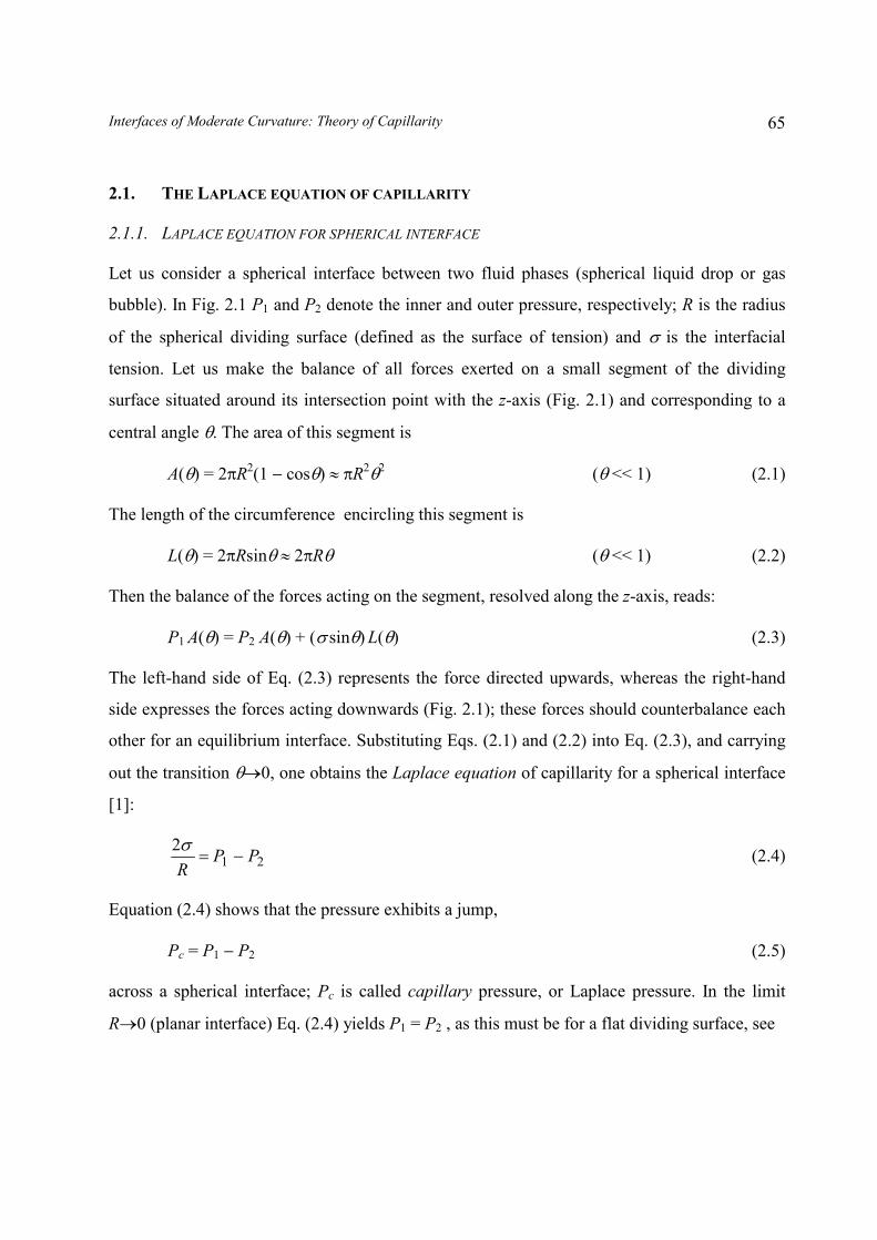
Derivation by minimization of the grand potential. Let us consider a two-phase fluid

system confined in a box of volume V, see Fig. 2.2. The volumes of the two phases are V1 and

V2 ; we have V1 + V2 = V. We assume also that the chemical potentials of all components in the

system are kept constant. Then the equilibrium state of the system corresponds to a minimum

of the grand thermodynamic potential, � [2-4]:

� � ��

1 2

21V V

AdVPdVP � (2.6)

where A is the area of the interface; the pressures P1 and P2 depend on the vertical coordinate z

due to the effect of gravity:

�

� �sinRP1

P2

Rsin�

� �sin

�

��

�

z


Fig. 2.2. Sketch of a two-phase system composed of phases 1 and 2, which occupy volumes V1 and V2,respectively; z = u(x,y) is the equation of the phase boundary.

P1(z) = P10 � �1gz, P2(z) = P20 � �2gz, (2.7)

P10 and P20 are constants, �1 and �2 are the mass densities of the two neighboring fluids, and g

is the acceleration due to gravity. Let z = u(x,y) to be the equation describing the shape of the

interface. Then the area of the interface is

yuu

xuuuudydxA yx

Ayx

�

�

�

�� ,,1

0

22 (2.8)

A0 is the projection of the interface on the coordinate plane xy. In addition, one derives

,)()(,)()( 2),(

21

),(

01

0101

zPdzdydxdVzPzPdzdydxdVzPA

b

yxuVA

yxu

V� �� (2.9)

where z = 0 and z = b are the lower and the upper side of the box (Fig. 2.2). The substitution of

Eqs. (2.8) and (2.9) into Eq. (2.6) yields

� �),(),,(),,(0

yxuyxuyxuLdxdy yxA�� (2.10)

where

��

b

uyx

u

yx uudzzPdzzPuuuL 222

01 1)()(),,( � (2.11)

0

phase 1

phase 2

x

V2

V1

u x,y( )

z

b

Chapter 268

Equations (2.10) and (2.11) show that the grand potential � depends as a functional on the

interfacial shape u(x,y). Then the necessary condition for minimum of � is given by the known

Euler equation [5,6]:

0��

yx uL

yuL

xuL

�

�

�

�

�

�

�

�

�

� (2.12)

Differentiating Eq. (2.11) one obtains

)()( 21 uPuPuL

��

�

�(2.13)

Next, differentiating Eq. (2.11) one can derive

��

�

�

�

�

�

�

� HuL

yuL

x yx2�� (2.14)

where we have used the notation

��

�

�

��

�

�

��

��

2II

IIII

12

u

uH (2.15)

yx yx�

�

�

� ee �� II (2.16)

Here �II is the two-dimensional gradient operator in the plane xy; H defined by Eq. (2.15) is a

basic quantity in differential geometry, which is termed mean curvature of the surface [5,7,8].

Note that Eq. (2.15) is expressed in a covariant form and can be specified for any type of

curvilinear coordinates in the plane xy (not only Cartesian ones). Substituting Eqs. (2.13) and

(2.14) into Eq. (2.12) we obtain a general form of Laplace equation of capillarity [1]:

2H� = P2(u) � P1(u) (Laplace equation) (2.17)

When the pressures P1 and P2 are dependent on the position in space, as it is in Eq. (2.7), their

values at the interface enter the Laplace equation; in such a case the capillary pressure, Pc �

P1(u) � P2(u), varies throughout the interface.


Various forms of Laplace equation. The mean curvature can be expressed through the

two principle radii of curvature of the surface, R1 and R2 [5,7]:

��

��

��

21

1121

RRH (2.18)

Combining Eqs. (2.17) and (2.18) one obtains another popular form of Laplace equation [9]:

� ��

��

��

21

11RR

= P1(u) � P2(u) (Laplace equation) (2.19)

For a spherical interface the two principal radii of curvature are equal, R1 = R2 = R, and then

Eq. (2.19) reduces to Eq. (2.4). The original form of Eq. (2.17), published by Laplace in 1805,

can be obtained if the right-hand side of Eq. (2.15) is expressed in Cartesian coordinates and

the differentiation is carried out [1]:

� � � �� 2/322

22

1

121

yx

yyxyxxyxxy

uu

uuuuuuu

��

��

= [P2(u) � P1(u)]/� (2.20)

Here uxx, uxy and uyy denote the respective second derivatives of u(x,y). One sees that in general

the Laplace equation, Eq. (2.20), is a second order non-linear partial differential equation for

determining the shape of the fluid phase boundary, u(x,y). The way we derived Eq. (2.20)

shows that its solution, u(x,y), minimizes the grand thermodynamic potential, �, and

consequently, corresponds to the state of mechanical equilibrium of the system. For interfaces

of rotational or translational symmetry Eq. (2.20) reduces to an ordinary differential equation

(see below), which is much easier to solve.

If the curved interface in Fig. 2.2 has translational symmetry along the y-axis, i.e. z = u(x), then

uy = 0, uxy = uyy = 0, and Eq. (2.20) reduces to:

� � 2/321 x

xx

u

u

�

= (P2 � P1)/� (translational symmetry) (2.21)

If the curved interface has rotational symmetry around the z-axis (axial symmetry), then it is

convenient to introduce polar coordinates (r,�) in the plane xy. Due to the axial symmetry the

Chapter 270

equation of the interface has the form z = u(r). Then introducing polar coordinates in Eq. (2.15)

one can bring Eq. (2.17) into the form [10]:

� � ��

��

�

�2/121

1

r

r

u

urrd

dr

= (P2 � P1)/� (rotational symmetry) (2.22)

where ur � du/dr. Sometimes it is more convenient to work in terms of the inverse function of

z = u(r), that is r = r(z). In such a case Eq. (2.22) can be transformed in an equivalent form

[10,11]:

2

212

2/122/32 ,,)1(

1)1( zd

rdrzdrdr

PPrrr

rzzz

zz

zz �

��

��

��

(2.23)

Two equivalent parametric forms of Laplace equation are often used for analytical and

numerical calculations [10,11]:

rdzdP

rrdd c

�� =tan,sinsin�

�

�� (2.24)

(the angle � can be defined with both positive or negative sign) and

��

�

� sin,cos,sin��

sdzd

sdrd

rP

sdd c (2.25)

Here � is the meniscus running slope angle and s is the arc length along the generatrix of the

meniscus z = z(r); Pc is the capillary pressure defined by Eq. (2.7); the sign of Pc is to be

specified for every given interface. Equations (2.25) represent a set of three equations for

determining the functions �(s), r(s) and z(s), which is especially convenient for numerical

integration [11]; note that Eq. (2.24) may create numerical problems at the points with

tan� = �, like the points on the “equator” of the fluid particle in Fig. 2.3.

The Laplace equation can be generalized to account for such effects as the interfacial bending

elasticity and shearing tension; such a generalization is important for interfaces and membranes

of low tension and high curvature and can be used to describe the configurations of red blood

cells, see Chapters 3 and 4.


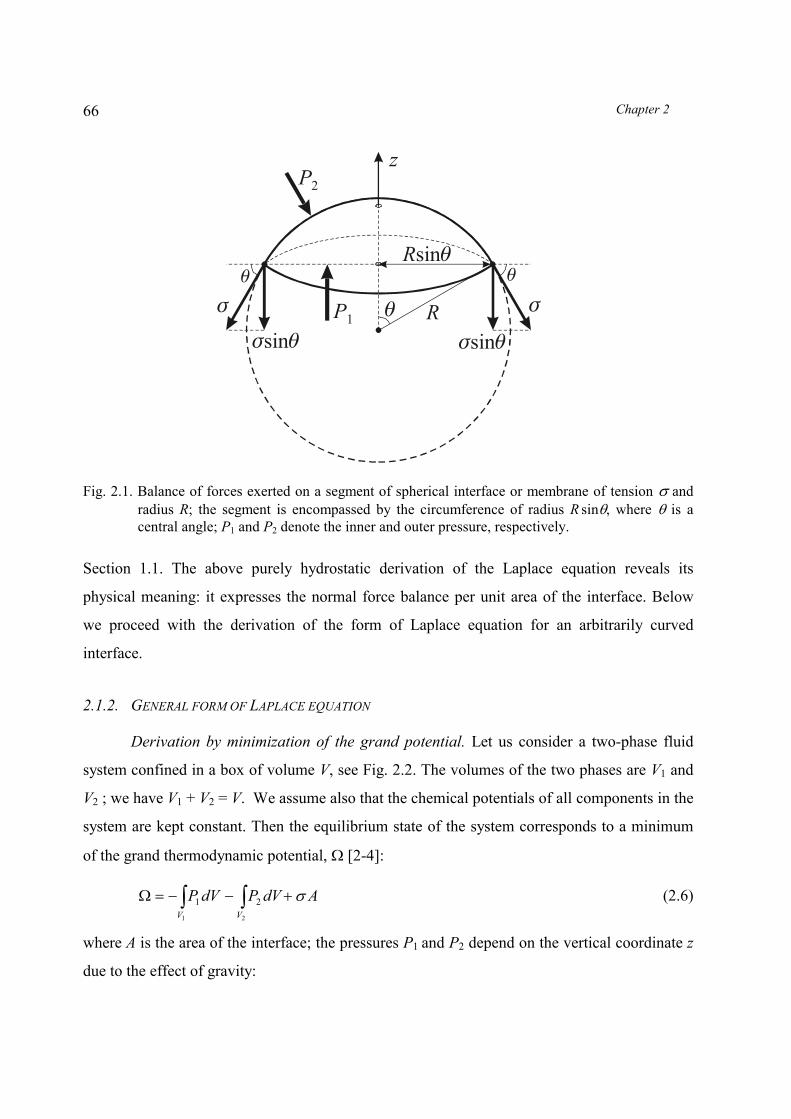
Fig. 2.3. Cross-section of a light fluid particle (bubble or droplet) from Phase 1, which is attached tothe boundary between Phases 2 and 3. The equations of the boundaries between phases 1-2, 1-3 and 2-3 are denoted by u(r), v(r) and w(r), respectively; �c, � and �c are slope angles of therespective phase boundaries at the contact line, which intersects the plane of the drawing inthe point (rc,zc); �(r) is a running slope angle; R is “equatorial” radius and Rf is the curvatureradius of the surface v(r), which can be a thin film of Phase 2, intervening between Phases 1and 3.

2.2. AXISYMMETRIC FLUID INTERFACES

Very often the boundaries between two fluid phases (the capillary menisci) have rotational

(axial) symmetry. An example is the fluid particle (drop or bubble) attached below an interface,

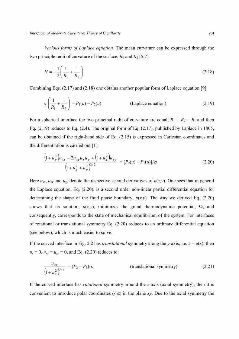
Fig. 2.4. Menisci formed by the liquid around two vertical coaxial cylinders of radii R1 and R2:(I) Meniscus meeting the axis of revolution; (II) Meniscus decaying at infinity; (III) Meniscusconfined between the two cylinders; hr is the capillary rise in the inner cylinder; hc and �c arethe elevation and the slope angle of Meniscus II at the contact line r = R2.

phase 3

phase 2 phase 1

�c

�c

rc

zc

r

�

�( )r

u r( )

w r( )

v r( )

0

RRf

z

ezer

r

Chapter 272

which is depicted in Fig. 2.3: all interfaces, u(r), v(r) and w(r), have axial symmetry. In general,

there are three types of axially symmetric menisci corresponding to the three regions denoted in

Fig. 2.4: (I) Meniscus meeting the axis of revolution, (II) Meniscus decaying at infinity, and

(III) Meniscus confined between two cylinders, 0 < R1 < r < R2

< ; see e.g. Ref. [10,12]. These

three cases are separately considered below.

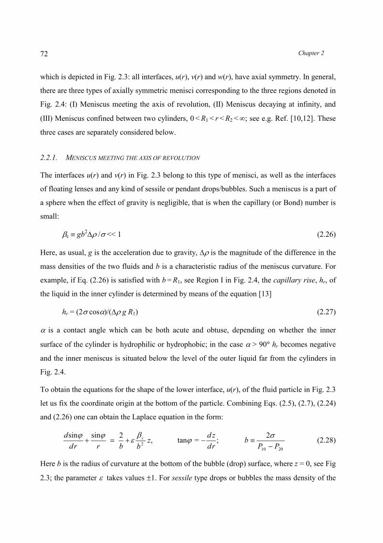
2.2.1. MENISCUS MEETING THE AXIS OF REVOLUTION

The interfaces u(r) and v(r) in Fig. 2.3 belong to this type of menisci, as well as the interfaces

of floating lenses and any kind of sessile or pendant drops/bubbles. Such a meniscus is a part of

a sphere when the effect of gravity is negligible, that is when the capillary (or Bond) number is

small:

�c � gb2� /� << 1 (2.26)

Here, as usual, g is the acceleration due to gravity, � is the magnitude of the difference in the

mass densities of the two fluids and b is a characteristic radius of the meniscus curvature. For

example, if Eq. (2.26) is satisfied with b = R1, see Region I in Fig. 2.4, the capillary rise, hr, of

the liquid in the inner cylinder is determined by means of the equation [13]

hr = (2� cos�)/(� g R1) (2.27)

� is a contact angle which can be both acute and obtuse, depending on whether the inner

surface of the cylinder is hydrophilic or hydrophobic; in the case � > 90� hr becomes negative

and the inner meniscus is situated below the level of the outer liquid far from the cylinders in

Fig. 2.4.

To obtain the equations for the shape of the lower interface, u(r), of the fluid particle in Fig. 2.3

let us fix the coordinate origin at the bottom of the particle. Combining Eqs. (2.5), (2.7), (2.24)

and (2.26) one can obtain the Laplace equation in the form:

20102

2;=tan,2sinsinPP

brdzdz

bbrrdd c

�

��

��

�� (2.28)

Here b is the radius of curvature at the bottom of the bubble (drop) surface, where z = 0, see Fig

2.3; the parameter � takes values �1. For sessile type drops or bubbles the mass density of the


fluid particle (Phase 1) is smaller than that of Phase 2, �1 < �2, and � = +1; for pendant type

drops/bubbles �1 > �2 and � = �1. The definition of the sign of tan� in Eq. (2.28) leads to

� = � at z = 0. (2.29)

Equations (2.28) allow one to determine the meniscus profile in a parametric form, that is

r = r(�) and z = z(�). Let us consider three cases corresponding to different values of the

capillary number �c.

(i) No gravity deformation: �c = 0. Such is the case of small fluid particles (drops,

bubbles) for which the gravitational deformation can be neglected. In this case the only solution

of the Laplace equation, Eq. (2.28), is a spherical meniscus:

br )(� = sin� ;

bz )(� = 1 + cos�. (2.30)

If the boundaries of small fluid particles or biological cells have a shape, which is different

from spherical, this is an indication about the presence of an effect of the interfacial

(membrane) bending elasticity, see Chapter 3.

(ii) Small gravity deformation: �c << 1. In this case the solution of Eq. (2.28) can be

obtained as truncated asymptotic expansions with respect to the powers of �c, see Ref. [14]:

��

��

��

��

��

�

��

��

��

��

��

2cot

2cot1sin

2sinlnsincos

sin2sin2

cotsin)(

291

21

312

92

21

432

21

61

31

��

��

��

��

c

cbr

(2.31)

� ��

��

��

��

� cos12

sinlnsincos1)(21

322

31

cbz (15�

� � � 180�) (2.32)

For �c �

0 Eqs. (2.31) and (2.32) reduce to Eq. (2.30). Equations (2.31) and (2.32) are

applicable with a good accuracy for 15� < � � 180�, see Refs. [14,15] for details. In the case

when 0� �

� � 15� instead of Eqs. (2.31) and (2.32) one can use the following asymptotic

expansions [14,15]:

Chapter 274

� �)(

2354814410827 2

24

33257

cccc O

pppppp

pbr

��

��

�

��

�� (2.33)

)(e2

ln2 232

21

cc Oppbz

�� (0� � � � 15�) (2.34)

where e is the Napier number, ln(e) = 1, and � �cp �� 382

21 �� , see Ref. [15] for more

details.

Other approximate solutions of Laplace equation can be found in Refs. [11,16]. For example, if

the meniscus slope is small, ur2 << 1, Eq. (2.22) reduces to a linear differential equation of

Bessel type, whose solution reads

z(r) = u(r) = 2[I0(qr) � 1]/(bq2), q � (� g/ )1/2, ur2 << 1 (2.35)

where I0(x) is the modified Bessel function of the first kind and zeroth order [5,17,18].

(iii) The gravity deformation is considerable and �c is not a small parameter. In this

case one can integrate numerically the Laplace equation in its parametric presentation,

Eq. (2.25).

Despite the fact that in the presence of gravitational deformation the Laplace equation has no

exact analytical solution, it is curious to note that there is an exact formula for the volume of a

sessile or pendant drop (bubble), irrespective of the magnitude of the gravitational deformation.

For example, the volume Vl of the lower part of the drop (bubble) in Fig. 2.3, that is comprised

between the planes z = 0 and z = zc , is

��

cc c z

c

z z

c

zr

dzdrzrzdzrzzrdzdrrdzdV

0

22

0 0 0

2)(

01 )(2)( ��

�

(2.36)

Here � denotes the azimuthal angle in the plane xy, r = r(z) is the generatrix of the interfacial

profile, rc is the radius of the contact line (Fig. 2.3); at the last step in Eq. (2.36) we have

integrated by parts. On the other hand, Eq. (2.28) can be expressed in the form

rzqrb

rdrd 22)sin( �� (2.37)


where q is defined by Eq. (2.35). Next, one multiplies Eq. (2.37) by dr/dz and integrates for

0 � z � zc; in view of Eq. (2.29) the result reads:

��

czc

cc dzdrzrzdzq

br

r0

22

)(sin �� (2.38)

The integral in Eqs. (2.36) and (2.38) cannot be solved analytically; however, this integral can

be eliminated between these two equations to obtain

��

�

�

��

�

�� cc

ccc r

br

qrzV �

�

�� sin2 2

22

1 (2.39)

where �c is the value of the slope angle � at z = zc, see Fig. 2.3. Similar expression can be

obtained also for the volume V2 of the upper part of the fluid particle in Fig. 2.3, that part

situated above the plane z = zc.

2.2.2. MENISCUS DECAYING AT INFINITY

Examples are the outer meniscus, z = w(r) in Fig. 2.3 and the meniscus in the outer Region II in

Fig. 2.4. In this case the action of gravity cannot be neglected insofar as the gravity keeps the

interface flat far from the contact line. Let z = 0 be the equation of the aforementioned flat

interface. Then P10 = P20 in Eq. (2.7) and the capillary pressure is Pc = � gz; the Laplace

equation (2.22) for the function z(r) takes the form:

� � � �zq

zr

z

z

z

r

r

r

rr 22/122/32 11

�

�

�

�

, 2

2

,dr

zdzdrdzz rrr �� (2.40)

Equation (2.40) has no closed analytical solution. The region far from the contact line has

always small slope, zr2 << 1. In this region Eq. (2.40) can be linearized and reduces to a

modified Bessel equation; in analogy with Eq. (2.35) one derives

z(r) = A K0 (qr) (zr2 << 1) (2.41)

where A is a constant of integration and K0(x) is the modified Bessel function of the second

kind and zeroth order [5,17,18]. The numerical integration of Eq. (2.40) can be carried out by

Chapter 276

using Eq. (2.41) as a boundary condition, together with zr = �qAK1(qr) for some appropriately

fixed r >> q�1 [11]; the constant A is to be determined from the boundary condition at r = R2.

Approximate analytical solutions of the problem are available [14,19�21]. For the case, when

the radius of the contact line R2 (Fig. 2.4) is much smaller than the characteristic capillary

length, q�1, Derjaguin [19] has derived an asymptotic formula for the elevation of the contact

line at the outer surface of the cylinder r = R2:

hc = �R2 sinc ln[qR2

�e

(1 + cosc)/4], (qR2 )2 << 1 (2.42)

Here c is the meniscus slope angle at the contact line (Fig. 2.4), q is defined by Eq. (2.35) and

�e = 1.781 072 418... is the Euler constant [17]. Note that Derjaguin’s formula (2.42) is valid

not only in the case 0 �

c

�

90�, but also in the case 90� �

c

�

180�, in which the meniscus has

Fig. 2.5. Sketch of a circular hole in a liquid wetting film of thickness hc on a solid substrate; �c is thecontact angle and r0 is the radius of the “neck” of the meniscus.

a neck, see e.g. Fig. 2.5. If the condition (qR2 )2 << 1 is satisfied, the constant A in Eq. (2.41)

can be determined [19,14]:

z(r) = R2 sinc K0(qr) zr2 << 1, (qR2 )2 << 1 (2.43)

Particles floating on a fluid interface of entrapped in a liquid film usually create small

interfacial deformations, for which Eqs. (2.42) and (2.43) are applicable. These equations will

be used below in this book to describe quantitatively the lateral capillary forces due to the

overlap of the interfacial deformations (menisci) formed around such particles.

�c

hcr0

r

z

0


If the condition zr2 << 1 is not fulfilled close to the cylinder r = R2, in this region one can use an

alternative “inner” asymptotic expression [14],

z(r) = ��

�

��

��

�

� ��

�

�

�

cccc R

rh��

�sin

1arccosh sin

arccosh sin2

(qR2)2 << 1 (2.44)

In Eq. (2.44) r � R2 and hc is given by Eq. (2.42); arccosh x = ln[x + (x2 �

1)1/2]; Eq. (2.44) has

meaning for z > 0. For large values of r Eq. (2.44) predicts negative values of z(r), which

indicates that this asymptotic formula is out of the region of its validity. Higher order

correction terms in Eqs. (2.42)�(2.44) are derived in Refs. [14,20].

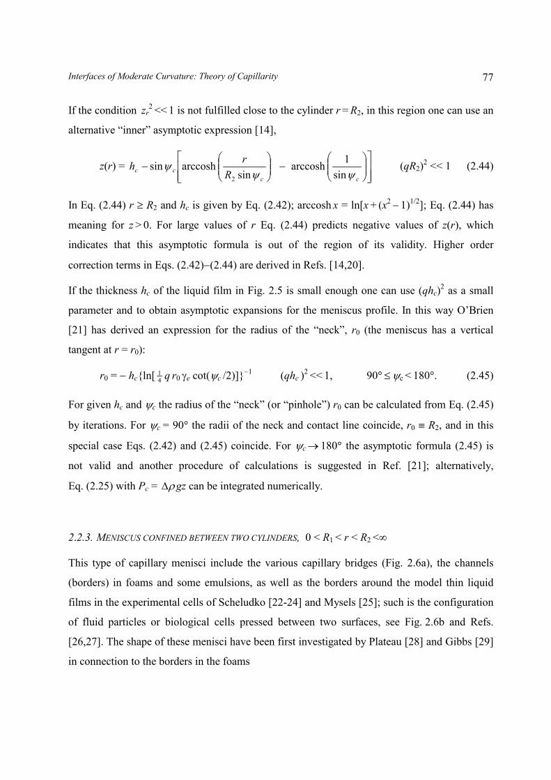
If the thickness hc of the liquid film in Fig. 2.5 is small enough one can use (qhc)2 as a small

parameter and to obtain asymptotic expansions for the meniscus profile. In this way O’Brien

[21] has derived an expression for the radius of the “neck”, r0 (the meniscus has a vertical

tangent at r = r0):

r0 = � hc{ln[ 41 q r0

�e cot(c /2)]}�1 (qhc )2 << 1, 90�

� c

< 180�. (2.45)

For given hc and c the radius of the “neck” (or “pinhole”) r0 can be calculated from Eq. (2.45)

by iterations. For c = 90� the radii of the neck and contact line coincide, r0 � R2, and in this

special case Eqs. (2.42) and (2.45) coincide. For c �

180� the asymptotic formula (2.45) is

not valid and another procedure of calculations is suggested in Ref. [21]; alternatively,

Eq. (2.25) with Pc = � gz can be integrated numerically.

2.2.3. MENISCUS CONFINED BETWEEN TWO CYLINDERS, 0 < R1 < r < R2 <

This type of capillary menisci include the various capillary bridges (Fig. 2.6a), the channels

(borders) in foams and some emulsions, as well as the borders around the model thin liquid

films in the experimental cells of Scheludko [22-24] and Mysels [25]; such is the configuration

of fluid particles or biological cells pressed between two surfaces, see Fig. 2.6b and Refs.

[26,27]. The shape of these menisci have been first investigated by Plateau [28] and Gibbs [29]

in connection to the borders in the foams

Chapter 278

If the gravitational deformation of the meniscus cannot be neglected, the interfacial shape can

be determined by numerical integration of Eq. (2.25), or by iterative procedure [30]. If the

meniscus deformation caused by gravity is negligible, analytical solution can be found as

described below. Equation (2.24) can be presented in the form

� ��

�2

,2sin 2111

PPkrkr

drd �

�� (2.46)

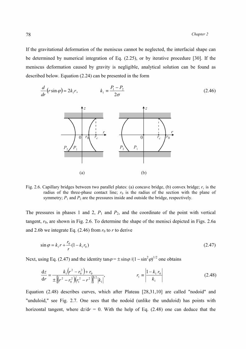
Fig. 2.6. Capillary bridges between two parallel plates: (a) concave bridge, (b) convex bridge; rc is theradius of the three-phase contact line; r0 is the radius of the section with the plane ofsymmetry; P1 and P2 are the pressures inside and outside the bridge, respectively.

The pressures in phases 1 and 2, P1 and P2, and the coordinate of the point with vertical

tangent, r0, are shown in Fig. 2.6. To determine the shape of the menisci depicted in Figs. 2.6a

and 2.6b we integrate Eq. (2.46) from r0 to r to derive

)1(sin 010

1 rkrrrk �� (2.47)

Next, using Eq. (2.47) and the identity tan� = � sin� /(1 �

sin2�)1/2 one obtains

� �� 1

011

12122

12

02

02

02

1 1,

dd

krk

rkrrrr

rrrkrz �

�

��

�� (2.48)

Equation (2.48) describes curves, which after Plateau [28,31,10] are called "nodoid" and

"unduloid," see Fig. 2.7. One sees that the nodoid (unlike the unduloid) has points with

horizontal tangent, where dz/dr = 0. With the help of Eq. (2.48) one can deduce that the


meniscus generatrix is a part of nodoid for k1r0 � (�, 0)�(1, �), whereas the meniscus

generatrix is a part of unduloid for k1r0 � (0, 1).

Fig. 2.7. Typical shape of the curves of Plateau: (a) nodoid, (b) unduloid. The curves are confinedbetween two cylinders of radii R1 and R2.

In the special case k1r0 = 1 the meniscus is spherical. In the other special case, k1r0

= 0, the

meniscus has the shape of catenoid, i.e.

� � )0(,1ln 12

000 ��

�� krrrrrz (2.49)

Qualitatively, the catenoid looks like the meniscus depicted in Fig. 2.6a; it corresponds to zero

capillary pressure and zero mean curvature of the interface (Pc = 0 and H = 0). In this case H = 0

because the two principle curvatures have equal magnitude, but opposite sign, at each point of

the catenoid. This is the reason why it is called also “pseudosphere”.

The meniscus has a "neck" (Fig. 2.6a) when k1r0 � (�, 1/2); in particular, the generatrix is

nodoid for k1r0 � (�, 0), catenoid for k1r0 = 0, and unduloid for k1r0 � (0, 1/2). For the

configuration depicted in Fig. 2.6a one has r1 > r0 (in Fig. 2.7 R1

= r0, R2 = r1) and Eq. (2.48) can

be integrated to yield

Chapter 280

� � � � � � � �1022

12

02

11111110 ,))((1,Esgn,F rrrrrrr

rrqkrqrrz ��

��

��

�

��

�� (2.50)

where sng x denotes the sign of x, q�

= (1 �

r02 �r1

2 )�� , sin1 = q�

��(1 �

r02 �r2 )��; F(, q) and

E(, q) are the standard symbols for elliptic integrals, respectively, of the first and the second

kind [5,17,18]:

� � ��

�

�

� �

��

��

0 0

22

22sin1),(E,

sin1),(F dqq

q

dq (2.51)

A convenient numerical method for computation of F(, q) and E(, q) is the method of the

arithmetic-geometric mean, see Ref. [18], Chapter 17.6.

The meniscus has a "haunch" (Fig. 2.6b) when k1r0 � (1/2, �); in particular, the generatrix is

unduloid for k1r0 �

(1/2, 1), circumference for k1r0 = 1, and nodoid for k1r0

�

(1, �). For the

configuration depicted in Fig. 2.6b one has r0 > r1 (in Fig. 2.7 R1 = r1, R2

= r0) and Eq. (2.48)

can be integrated to yield

� � � � � � � �� 012202210 ,,E,F1 rrrqrqkrrz �� (2.52)

where q�

= (1�r�2 �r�2 )��, sin� = q�

��(1 �

r2 �r�2 )��. More about capillary bridges can be found

in Chapter 11. Equation (2.52) has been also used [26,27] to describe the shape of drops and

blood cells entrapped in liquid films.

2.3. FORCE BALANCE AT A THREE-PHASE-CONTACT LINE

2.3.1. EQUATION OF YOUNG

As discussed in Section 2.1.2, the Laplace equation is a differential equation, which needs

boundary conditions to obtain an uniquely defined solution for the shape of the interface. In

Section 2.1.1 we demonstrated that the Laplace equation can be derived as a necessary

condition for minimum of the grand thermodynamic potential � by using variations in the

meniscus shape u(x,y) at fixed boundaries. In addition, the boundary conditions for Laplace

equation can be derived in a similar way by using variations in the meniscus shape at mobile

boundaries, see e.g. [8,32-34].


Fig. 2.8. Sketch of a two-phase system composed of phases 1 and 2 occupying volumes V1 and V2separated by an interface of equation z = u(x); A1 and A2 are the contact areas of therespective phases with the right-hand side wall; � is contact angle; �u(x) and �u1 representvariation in the shape of the interface and in the position of the contact line, respectively.

Let us consider again a two-phase system closed in a box of volume V = V1 + V2, see Fig. 2.8.

For the sake of simplicity, let us assume that the meniscus has a translational symmetry along

the y-axis; then the meniscus profile is z = u(x). Let the right-hand-side wall of the box

(Fig. 2.8) be a vertical solid plate situated at x = x1. We consider variations, �u(x), of the

meniscus profile for movable contact line at the vertical wall at x = x1. The grand potential �

can be expressed in the form

� � ��

1 2

21V V

AdVPdVP � + �1s A1 + �2s

A2 (2.53)

where A1 and A2 are the contact areas of the vertical wall with phase 1 and 2, respectively

(Fig. 2.8); �1s and �2s can be interpreted as surface excess densities of � for the boundaries

solid / phase 1 and solid / phase 2. Since the meniscus has translational symmetry, one can write

,)()(,)()( 2)(0

20

1

)(

01

1

1

1

1

zPdzdxldVzPzPdzdxldVzPb

xu

x

V

x xu

V�� (2.54)

0

(1)

(2)

xx1

V2

V1

A2

A1

�

A

u x( )�u x( ) �u1

z

b

Chapter 282

where l is the length of the meniscus along the y-axis; z = 0 and z = b are the lower and the

upper side of the box (Fig. 2.8). The area of the boundary between phases 1 and 2 is

xuuudxlA x

x

x�

�� ,1

1

0

2 (2.55)

Let the variation �u(x) of the meniscus profile is accompanied by a variation �u1 of the position

of the contact line at the vertical wall at x = x1. Then �A1 = � �A2 = l �u1 and in view of Eqs.

(2.53)�(2.55) the first variation of the grand potential � can be expressed in the form:

� � 1210

)(1

uldxLl ss

x

�� (2.56)

where

��

b

ux

u

x udzzPdzzPuuL 22

01 1)()(),( � (2.57)

Differentiating Eq. (2.57) one obtains

xdud

uLu

uLL

x

)(��

��

�

�� (2.58)

Next, we integrate by parts the last term in Eq. (2.58):

dxuuL

dxdu

uLxd

xdud

uL x

xxxx

x

x

��

��

�

��

�

�

��

��

��

�

� ��

�

�

��

�

1

1

1

01

0

)( (2.59)

Combining Eqs. (2.56)�(2.59) one derives

1210 1

1

uluLdxu

uL

dxd

uLl ss

xxx

x

x

��

��

�

�

�

��

��

�

�

��

�

��

��

��

�

��

�

��

��

�

� (2.60)

We already know that the meniscus profile satisfies the Laplace equation, Eq. (2.21), which is

equivalent to the equation 0��

��

��

xuL

dxd

uL

�

�

�

� . Hence, the integral term in Eq. (2.60) is equal

to zero. Furthermore, the necessary condition for minimum is �� = 0, and �u1 is an

independent and arbitrary variation. Then the term multiplying �u1 in Eq. (2.60) must be equal

to zero:


021

1

��

��

�

ssxxxu

L��

�

� (2.61)

Using Eq. (2.57) and the identity ux = tan�, where � is the running slope angle, one can derive:

��

��

�

� sintan1

tan1 22

�

�

�

�

�

x

x

x u

uuL (2.62)

Finally, in Eq. (2.62) we set x = x1 and take into account that � � �� cossin1�

�xx , where � is

the contact angle (Fig. 2.8); then Eq. (2.61) transforms into the Young [35] equation:

�2s � �1s � � cos� (Young equation) (2.63)

An equivalent equation has been obtained by Dupré [36] in his analysis of the work of

adhesion. We derived Eq. (2.63) for the special case of meniscus of translational symmetry,

however, this equation has the same form for arbitrarily shaped meniscus and solid surface, see

e.g. Ref. [8].

The above derivation of Young equation, which is similar to the derivation of Laplace equation

in Section 2.1.1, implies that the Young equation expresses the balance of forces per unit

length of a three-phase-contact line, likewise the Laplace equation expresses the force balance

per unit area of a phase boundary. According to Gibbs [29] �1s and �2s can be interpreted as

surface tensions (forces per unit area): �1s and �2s oppose every increase of the “wet” area

(without any deformation of the solid) in the same way as � opposes every dilatation of the

interface between fluids 1 and 2; Gibbs termed �1s and �2s “superficial tensions”.

Equation (2.63), presented in the form cos� = (�2s � �1s)/�, shows that the contact angle � can

be expressed in terms of the three surface tensions, which in their own turn are determined by

the excess molecular interactions in the zone of the phase boundaries (Section 1.1.1).

Therefore, the magnitude of the equilibrium contact angle is determined by the intermolecular

forces.

It is worth noting that �� = 0 is only a necessary, but not sufficient, condition for a minimum

of the grand potential �. This condition is fulfilled also in the case of maximum and inflection

Chapter 284

point of �. Quite surprisingly, Eriksson & Ljunggren [37] established that for gas bubbles

attached to a hydrophobic wall the Young equation can correspond to a maximum of �, i.e. to

a state of unstable equilibrium. Further, in Ref. [38] the conditions for stable or unstable

attachment of a fluid particle (drop, bubble) to a solid wall have been examined.

The force interpretation of the Young equation is illustrated in Fig. 2.9a. One sees that Eq.

(2.63) represents the horizontal projection of the vectorial force balance

� + �1s + �2s + fR = 0 (2.64)

where the underlined sigma’s denote vectors, each of them being tangential to the respective

interface and normal to the contact line; fR is the vector of the bearing reaction, which is

normal to the surface of the solid substrate and counterbalances the vertical projection of the

meniscus surface tension:

fR = � sin� (2.65)

Equation (2.65) can be useful in the analysis of the forces applied to a particle, which is

attached to an interface (see below). Note that the thermodynamic interpretations of �, �1s and

�2s as surface excess densities of the grand thermodynamic potential � are completely

compatible with their mechanical interpretation as forces per unit length (Fig. 2.9a) insofar as

boundaries of a liquid phase are considered and deformations of the solid walls are neglected.

These two interpretations (as energy per unit area and force per unit length) are mutually

complementary, in spite of the fact that some authors favor the thermodynamic and other ones

� the mechanical interpretation. As already mentioned, Gibbs [29] interpreted �1s and �2s as

tensions opposing the increase of the wet area on the solid surface without any deformation of

the solid. On the other hand, differences between energy per unit area and force per unit length

appear if deformations of the solid surface take place, see e.g. Refs. [39-43]. Then the force per

unit length becomes a two-dimensional tensor, whereas the energy per unit area remains a

scalar, and consequently, these two quantities cannot be equal; the trace of the tensor (the

surface tension of the solid) is related to the excess surface energy per unit area by means of the

Shuttleworth equation [39-43]. Deformations of the solid phase are out of the conventional

capillary hydrostatics and thermodynamics, and will not be considered here.


Fig. 2.9. Force interpretation of (a) Young equation (2.64) and (b) the Neumann triangle (2.66); fR isthe bearing reaction of the solid substrate, which counterbalances the normal projection of thesurface tension, � sin�; � and � are contact angles.

2.3.2. TRIANGLE OF NEUMANN

Three-phase-contact line can be formed also when all the three phases are fluid: such is the

line of intersection of the menisci u(r), v(r) and w(r) in Fig. 2.3 (drop or bubble attached to an

interface) and Fig. 2.9b (liquid lens at a fluid phase boundary). In this case one can prove

(again by a variational method, see e.g. Refs. [32,33]) that the force balance per unit length of

the contact line is given by the Neumann [44] vectorial triangle:

�u + �v + �w = 0, (Neumann triangle) (2.66)

see Fig. 2.9b and Refs. [3,31,45,46]. In this case there are two independent contact angles: �

and �. Applying the known cosine theorem to the triangle in Fig. 2.9b one obtains:

�w2 = �u

2 + �v2 + 2�u�v cos� , �v

2 = �u2 + �w

2 + 2�u�w cos� , (2.67)

From Eq. (2.67) one determines [3,46-48]

wu

wuv

vu

vuw

��

��

��

��

2cos,

2cos

222222��

�

��

� (2.68)

fluid 1

fluid 2

(1)(2)

Neumanntriangle

(3)

(a) (b)

solid

�

�1s �2s �w

��

�

�w

�v

�v

�u

�u

fR

� �sin

u r( )

w r( )v r( )�

� �cos

Chapter 286

Equations (2.68) relate the contact angles � and � to the three interfacial tensions. Hence, we

again arrive to the conclusion that the magnitude of the contact angles is determined by the

intermolecular forces (which determine also the values of the sigma’s) and, moreover, the

contact angles do not depend on applied external fields such as gravitational or centrifugal.

Note however, that if a line tension is present at the contact line (Section 2.3.3), the contact

angle becomes (in principle) dependent on applied external fields as proven by Ivanov et al.

[32].

It must be emphasized that the above conclusions related to the physical nature of the contact

angles are valid only for the true, i.e. correctly defined, contact angles. Experimentally, by

means of some optical method the shapes of the interfaces at some distance from the contact

line are usually determined, and then by extrapolating them until they intersect the contact

angle is found, for review see e.g. Refs. [30,49,50]. The first problem encountered when this

procedure is carried out in practice is that the minimum distance from the contact line, at which

one can still obtain experimental information about the interfacial shape, is limited by the

magnification of the microscope [51]. The second problem is related to the transition region in

a narrow vicinity of the contact line in which the interactions between the three neighboring

phases affect the interfacial tensions and the shape of the interfaces. Although the width of the

transition region (it was estimated to 1 �m in Ref. [52]) is smaller than the resolution of the

optical methods, if some of the experimental points happen to lie there, this will again affect

the extrapolation procedure, and hence � the value of the macroscopic contact angle.

The only way to avoid these two errors is [32]: (i) to make sure that all experimental points

used lie outside of the transition region and (ii) to carry out the extrapolation of the surface in

such a way that its shape at all points satisfies the Laplace equation with the macroscopic value

of the surface tension.


2.3.3. THE EFFECT OF LINE TENSION

As discussed above, the true thermodynamic contact angle is subtended between the

extrapolated surfaces, which obey the Laplace equation. On the other hand, the interactions

between the phases (the disjoining pressure effects) in a vicinity of the three-phase-contact line

may lead to a deviation of the real interfacial shape from the extrapolated surface and to a

variation of the interfacial tensions in this narrow region. In such a case, to make the idealized

system (composed of uniform bulk phases and interfaces obeying the Laplace equation at

constant surface tension) equivalent to the real system, some excesses of the thermodynamic

parameters can be ascribed to the three-phase contact line. The excess linear density of the

grand thermodynamic potential � has the meaning of a line tension, likewise the excess surface

density of � is identified as the surface tension, see e.g. Ref. [53]. Furthermore, the line tension

can be interpreted as a force, directed tangentially to the contact line, just like the tension of a

stretched fiber or string [54].

For the first time the concept of line tension was formulated by Gibbs [29] in his theory of

capillarity. The thermodynamic theory of systems with line tension was developed by Buff and

Saltsburg [45], and Boruvka and Neumann [53]. The theory of line tension for systems

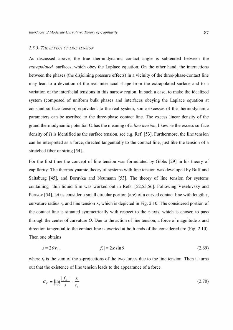
containing thin liquid film was worked out in Refs. [52,55,56]. Following Veselovsky and

Pertsov [54], let us consider a small circular portion (arc) of a curved contact line with length s,

curvature radius rc and line tension �, which is depicted in Fig. 2.10. The considered portion of

the contact line is situated symmetrically with respect to the x-axis, which is chosen to pass

through the center of curvature O. Due to the action of line tension, a force of magnitude � and

direction tangential to the contact line is exerted at both ends of the considered arc (Fig. 2.10).

Then one obtains

s = 2� rc , | fx | = 2� sin� (2.69)

where fx is the sum of the x-projections of the two forces due to the line tension. Then it turns

out that the existence of line tension leads to the appearance of a force

c

x

rsf �

��

��

�

||lim

0(2.70)

Chapter 288

Fig. 2.10. The line tension �, acting tangentially to a small portion (arc) of a curved contact line, leadsto the appearance of a force per unit length �� = �/rc, which is directed toward the center ofcurvature of the arc, point O; rc is the curvature radius of the considered elementary arc ofthe contact line.

acting per unit length of the contact line. In each point of the contact line this force, �� , is

directed toward the center of curvature (toward the center of the circumference, if the contact

line is circular). The above derivation is valid for any smooth curved line, insofar as every

small portion of such a line can be approximated with an arc of circumference [7].

If the effect of line tension is included into the Young equation, Eqs. (2.63) and (2.64) acquire

the more general form [57]:

css r

�

�� cos12 (2.71)

� + �1s + �2s + �� + fR = 0 (2.72)

In this case the contact line belongs to a solid surface and the force interpretation of � and �� is

similar to the interpretation of �1s and �2s given by Gibbs (see above); in particular, � can be

interpreted as a force, which opposes the extension of the perimeter of the wet zone in every

process of variation of the wet area without any deformation in the solid substrate.

0

rc�

� �

� �

�

rc

x

� �sin � �sin

O


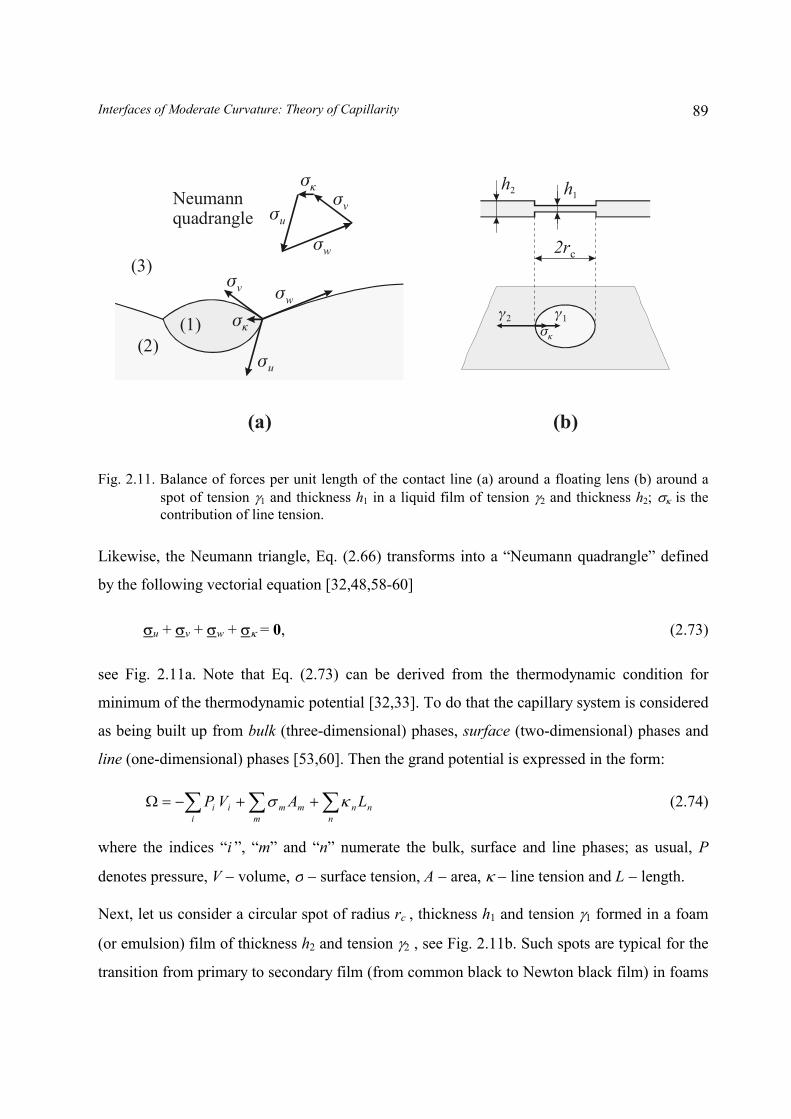
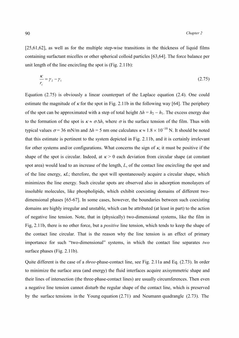
Fig. 2.11. Balance of forces per unit length of the contact line (a) around a floating lens (b) around aspot of tension �1 and thickness h1 in a liquid film of tension �2 and thickness h2; �� is thecontribution of line tension.

Likewise, the Neumann triangle, Eq. (2.66) transforms into a “Neumann quadrangle” defined

by the following vectorial equation [32,48,58-60]

�u + �v + �w + �� = 0, (2.73)

see Fig. 2.11a. Note that Eq. (2.73) can be derived from the thermodynamic condition for

minimum of the thermodynamic potential [32,33]. To do that the capillary system is considered

as being built up from bulk (three-dimensional) phases, surface (two-dimensional) phases and

line (one-dimensional) phases [53,60]. Then the grand potential is expressed in the form:

� � ��

i m nnnmmii LAVP �� (2.74)

where the indices “i ”, “m” and “n” numerate the bulk, surface and line phases; as usual, P

denotes pressure, V � volume, � � surface tension, A � area, � � line tension and L � length.

Next, let us consider a circular spot of radius rc , thickness h1 and tension �1 formed in a foam

(or emulsion) film of thickness h2 and tension �2 , see Fig. 2.11b. Such spots are typical for the

transition from primary to secondary film (from common black to Newton black film) in foams

(1)(2)

Neumannquadrangle

(3)

(a) (b)

�w

�w

�v

h� h

�

2rc

��

��

�v

�u

�u

��

��

��

Chapter 290

[25,61,62], as well as for the multiple step-wise transitions in the thickness of liquid films

containing surfactant micelles or other spherical colloid particles [63,64]. The force balance per

unit length of the line encircling the spot is (Fig. 2.11b):

12 ��

��

cr(2.75)

Equation (2.75) is obviously a linear counterpart of the Laplace equation (2.4). One could

estimate the magnitude of � for the spot in Fig. 2.11b in the following way [64]. The periphery

of the spot can be approximated with a step of total height h = h2 � h1. The excess energy due

to the formation of the spot is � � � h, where � is the surface tension of the film. Thus with

typical values � = 36 mN/m and h = 5 nm one calculates � � 1.8 � 10�10 N. It should be noted

that this estimate is pertinent to the system depicted in Fig. 2.11b, and it is certainly irrelevant

for other systems and/or configurations. What concerns the sign of �, it must be positive if the

shape of the spot is circular. Indeed, at � > 0 each deviation from circular shape (at constant

spot area) would lead to an increase of the length, L, of the contact line encircling the spot and

of the line energy, �L; therefore, the spot will spontaneously acquire a circular shape, which

minimizes the line energy. Such circular spots are observed also in adsorption monolayers of

insoluble molecules, like phospholipids, which exhibit coexisting domains of different two-

dimensional phases [65-67]. In some cases, however, the boundaries between such coexisting

domains are highly irregular and unstable, which can be attributed (at least in part) to the action

of negative line tension. Note, that in (physically) two-dimensional systems, like the film in

Fig, 2.11b, there is no other force, but a positive line tension, which tends to keep the shape of

the contact line circular. That is the reason why the line tension is an effect of primary

importance for such “two-dimensional” systems, in which the contact line separates two

surface phases (Fig. 2.11b).

Quite different is the case of a three-phase-contact line, see Fig. 2.11a and Eq. (2.73). In order

to minimize the surface area (and energy) the fluid interfaces acquire axisymmetric shape and

their lines of intersection (the three-phase-contact lines) are usually circumferences. Then even

a negative line tension cannot disturb the regular shape of the contact line, which is preserved

by the surface tensions in the Young equation (2.71) and Neumann quadrangle (2.73). The


Fig. 2.12. Balance of forces per unit length of the contact line of a small solid sphere attached to theplanar interface between the fluid phases 1 and 2; � is the interfacial tension, �1s and �2s arethe two solid-fluid tensions, �� is the line tension effect, fR is the bearing reaction of thesolid particle: fR + �� sin� = � sin�.

accumulated results for three-phase systems show that the line-tension term turns out to be only

a small correction, which can be (and is usually) neglected in Eqs. (2.71)�(2.73), see Section

2.3.4.

As an example for application of the Young equation (2.72) let us consider a small spherical

particle attached to the interface between two fluid phases, Fig. 2.12. We presume that the

weight of the particle is small and the particle does not create any deformation of the fluid

interface [68,69]. All forces taking part in Eq. (2.72) are depicted in Fig. 2.12, including the

normal projection, � sin�, of the interfacial tension. Its tangential projection, � cos�, is

counterbalanced by �2s + �� cos� � �1s in accordance with the Young equation. Then one could

conclude (erroneously!) that � sin� and/or �� sin� , which have non-zero projections along the

z-axis (Fig. 2.12), give rise to a force acting on the particle along the normal to the fluid

interface. If such a force were really operative, it would create a deformation of the fluid

interface around the particle, which would be in contradiction with the experimental

observations. Then a question arises: how to calculate correctly the net force exerted on a fluid

particle attached to an interface at equilibrium?

(1)

(2)

�1s

�2s

��

fR

� �sin

� �

z

Chapter 292

The rule (called sometimes the principle of Stevin), stems from the classical mechanics and it

is the following: The net force exerted on a particle originates only from phases, which are

outer with respect to the given particle: the pressure of an outer bulk phase, the surface tension

of an outer surface phase and the line tension of an outer line phase. (For example, if a particle

is hanging on a fiber, then the tension of the fiber has to be considered as the line tension of an

“outer line phase”.)

In our case (the particle in Fig. 2.12) the outer forces are the pressures in the two neighboring

fluid phases 1 and 2, and the surface tension, �, of the boundary between them. The integral

effect of their action gives a zero net force for the configuration depicted in Fig. 2.12 due to its

symmetry. Then there is no force acting along the normal to the interface and the latter will not

undergo a deformation in a vicinity of the particle. (Such a deformation would appear if the

particle weight and the buoyancy force were not negligible.)

On the other hand, the solid-fluid tensions, �1s and �2s, the tension �� due to line tension, and

the bearing reaction of the solid, fR, cannot be considered as outer forces. However, �1s , �2s

and �� also affect the equilibrium position of the particle at the interface insofar as they

(together with �) determine the value of the contact angle �, see Eq. (2.71).Additional

information can be found in Chapter 5 below, where balances of forces experienced by

particles attached to the boundary between two fluids are considered.

2.3.4. HYSTERESIS OF CONTACT ANGLE AND LINE TENSION

The experimental determination of line tension is often based on the fact, that the presence of a

�/rc term in Eqs. (2.71) and (2.73) leads (in principle) to a dependence of the contact angle �

on the radius of the contact line rc (�, �1s and �2s are presumably constants), see Refs. [70-79].

However, there is another phenomenon, the hysteresis of contact angle, which also leads to

variation of the contact angle, see e.g. Ref. [80]. Both phenomena may have a similar physical

origin [75].

The fact that a hysteresis of contact angle takes place with liquid menisci on a solid substrate

has been known for a long time [81,82]. It is an experimental fact that a range of stable contact

angles can be measured on a real solid surface. The highest of them is termed “advancing”, and


the lowest one � “receding” contact angle. The difference between the advancing and receding

angles is called “the range of hysteresis”, or shortly, “hysteresis” [83,84]. The widely accepted

qualitative explanation of this phenomenon is that the hysteresis is caused by the presence of

surface roughness and chemical heterogeneity of the real solid surfaces [75, 85-96]. From this

viewpoint, the Young equation is believed to be valid only for an ideal solid surface, which is

molecularly smooth, chemically homogeneous, rigid and insoluble [84].

However, hysteresis of contact angle can be observed even on an ideal solid surface if a thin

liquid film is formed in front of an advancing meniscus, or left behind a receding meniscus;

this was proven theoretically by Martynov et al. [97], see also Refs. [98,99]. In this case the

hysteresis is due to the action of an adhesive surface force within the thin film, which opposes

the detachment of the film surfaces and facilitates their attachment. Such forces are present

(and hysteresis is observed) not only in wetting films on a solid substrate, but also in free foam

and emulsion films stabilized by usual surfactants [100-102] or by proteins [99]. It turns out

that, as a rule, one observes hysteresis of contact angle and only with some special systems

hysteresis is completely missing. Such special systems can be liquid lenses on a fluid interface

[30, 103-107] or thin films without strong adhesive forces [108].

The occurrence of hysteresis is different for a completely fluid three-phase-contact line and for

a three-phase contact involving one solid phase: In the former case at complete equilibrium

(immobile contact line) an equilibrium contact angle is established [99-102]; in contrast, in the

latter case (in the presence of solid phase) it is practically impossible to figure out which angle,

could be identified as the equilibrium one within the range between the receding and advancing

angles.

Coming back to the line tension issue, in Fig. 2.13 we demonstrate, that in some cases the line

tension could be a manifestation of the hysteresis of contact angle. Let us assume that for some

value of the contact angle, � = �1, the Young equation (2.63) is satisfied (Fig. 2.13a). Due to

the hysteresis another metastable contact angle, �2, exists (�2 > �1, see Fig. 2.13b). From a

macroscopic viewpoint the force balance in Fig. 2.13b can be preserved if only a line tension

term, �� = �/rc, is introduced, see Eq. (2.71) with � = �2. Indeed, the surface tensions �, �1s

Chapter 294

Fig. 2.13. Sessile liquid drop on a solid substrate. (a) Balance of the forces acting per unit length of thecontact line, of radius rc ; � is the surface tension of the liquid, �1s and �2s are the tensions ofthe two solid-fluid interfaces, �1 is contact angle. (b) After liquid is added to the drop,hysteresis is observed: the contact angle rises to �2 at fixed rc ; the fact that the macroscopicforce balance is preserved (the contact line remains immobile) can be attributed to the actionof a line tension effect �� .

and �2s are the same in Figs. 2.13a and 2.13b, and the difference between the contact angles

(�2 > �1) can be attributed to the action of a line tension.

The interpretation of the contact-angle hysteresis as a line tension could be accepted, because,

as already mentioned, the two phenomena have a similar physical origin: local microscopic

deviations from the macroscopic Young-Laplace model in a narrow vicinity of the contact line.

When the meniscus advance is accompanied by an increase of the contact radius rc, a positive

line tension must be included in the Young equation to preserve the force balance (Fig. 2.13b).

In the opposite case, if the meniscus advance is accompanied by a decrease of rc, then a negative

line tension must be included in the Neumann-Young equation to preserve the force balance.

The shrinking bubbles, like that depicted in Fig. 2.3, correspond to the latter case and, really,

negative line tensions have been measured with such bubbles [109,110, 100-102]; see also the

discussion in Ref. [111].

Theoretical calculations, which do not take into account effects such as surface roughness or

heterogeneity, or dynamic effects with adhesive thin films, usually predict very small values of

the line tension from 10�11 to 10�13 N, see Table 2.1. On the contrary, the experiments which

deal with real solid surfaces, or which are carried out under dynamic conditions, as a rule give

much higher values of � (Table 2.1). The values of � in a given experiment often have variable

magnitude, and even � variable sign [70-73,100-102,109,110]. Moreover, the values of �

(a) (b)

��

�1s �1s��rc rc

�2s �2s��

��


determined in different experimental and theoretical works vary with 8 orders of magnitude

(Table 2.1).

Table 2.1. Comparison of experimental and theoretical results for line tension �.

Researchers Theory /

Experiment

System Value(s) of line tension� (N)

Tarazona & Navascues [112] Theory Solid-liquid-vaporcontact line

�2.6 to �8.2 � 10�11

Navascues & Mederos [113] Experiment Nucleation rate ofwater drops on Hg

�2.9 to �3.9 � 10�10

de Feijter & Vrij [52] Theory Foam films � �1 � 10�12

Kolarov & Zorin [114] Experiment Foam films �1.7 � 10�10

Denkov et al. [115] Theory Emulsion films �0.95 to �1.57 � 10�13

Torza and Mason [59] Experiment Emulsion films �0.6 to �5.8 � 10�8

Ivanov & coworkers[100-102, 109-111]

Experiment Foam film at the top ofshrinking bubbles

�1 � 10�7 to � 0

Wallace & Schürch[116,117]

Experiment Sessile drop onmonolayer

+1 to +2.4 � 10�8

Neumann & coworkers[118-121]

Experiment Sessile drops +1 to +6 � 10�6

Gu, Li & Cheng [122] Experiment Interface around a cone � +1 � 10�6

Nguyen et al. [123] Experiment Silanated glass sphereson water-air surface

+1.2 to +5.5 � 10�6

There could be some objections against the formal treatment of the contact angle hysteresis as a

line-tension effect. Firstly, some authors [124-126] interpret the hysteresis as an effect of static

friction (overcoming of a barrier), which is physically different from the conventional

molecular interpretation of line tension, see e.g. Ref. [112]. Secondly, a hysteresis of contact

angle can be observed also with a straight contact line (rc�); if such hysteresis is interpreted

as a line tension effect, one will obtain ��, but �� = �/rc will remain finite.

Chapter 296

If �� in the Neumann “quadrangle”, Eq. (2.73), is a manifestation of hysteresis, then �� is not

expected to vary significantly with the size of the particles (solid spheres, drops, bubbles,

lenses). On the other hand, rc can vary with many orders of magnitude. Consequently, if the

line tension effect in some system is a manifestation of a contact angle hysteresis, then one

could expect that the measured |� | = |�� | rc will be larger for the larger particles (greater rc)

and smaller for the smaller particles (smaller rc). Some of the reported experimental data

(Table 2.1) actually exhibit such a tendency. For example, in the experiments of Neumann and

coworkers [118-121] and Gu et al. [122] rc � 3 mm and one estimates an average value ��

1 mN/m; in the experiments of Ivanov and coworkers [100-102,109,110] the mean value of the

contact radius is rc � 35 �m and one estimates |��

| � 1.4 mN/m; in the experiment of Torza &

Mason [59] rc � 15 �m in average and then |��

| � 2 mN/m; in the experiments of Navascues &

Mederos [113] rc � 23 nm and one obtains |��

| � 20 mN/m. One sees, that in contrast with |� |,

which varies with many orders depending on the experimental system, |��

| exhibits a relatively

moderate variation. Then a question arises whether � or �� is a better material parameter

characterizing the linear excess at the three-phase contact line.

In the experiments with slowly diminishing bubbles from solutions of ionic surfactant [100-

102] it has been firmly established that the shrinking of the contact line is accompanied by a

rise (hysteresis) of the contact angle, �, and appearance of a significant negative line tension, �.

When the shrinking of the contact line was stopped (by control of pressure), both � and |� |

relaxed down to their equilibrium values, which for � turned out to be zero in the framework of

the experimental accuracy (�1.5 � 10�8 N). This effect was interpreted [100-102,111] as a

“dynamic” line tension related to local deformations in the zone of the contact line, which are

due to the action of attractive (adhesive) forces opposing the detachment of the film surfaces in

the course of meniscus advance. Arguments in favor of such an interpretation are that a

measurable line tension effect is missing in the case of (i) receding meniscus (expanding

bubbles) [100-102] and (ii) shrinking bubbles from nonionic surfactant solution [108]. In the

latter case the adhesive surface forces in the film are negligible.

Finally, let us summarize the conclusions stemming from the analysis of the available

experimental and theoretical results for the line tension:


1) The line tension of three-phase-contact-lines can vary by many orders of magnitude

depending on the specific system, configuration (contact-line radius) and process (static or

dynamic conditions). The sign of line tension could also vary, even for similar systems [70-73].

In some cases this could be due to the fact, that the measured line tension is a manifestation of

hysteresis of contact angle; in this case the variability of the magnitude and sign of the line

tension is connected with the indefinite value of the contact angle. Hence, unlike the surface

tension, the line tension, �, strongly depends on the geometry of the system and the occurrence

of dynamic processes. This makes the theoretical prediction of line tension a very hard task and

limits the importance and the applicability of the experimentally determined values of � only to

the given special system, configuration and process.

2) The line tension of three-phase-contact lines is usually a small correction (an effect

of secondary importance) in the Young equation or Neumann triangle, and it could be

neglected without a great loss of accuracy.

3) In contrast, the line tension of the boundary between two surface phases (see e.g.

Fig. 2.11b) is an effect of primary importance, which determines the shape and the stability of

the boundaries between domains (spots) in thin liquid films and Langmuir adsorption films.

2.4. SUMMARY

The pressure exhibits a jump on the two sides of a curved interface or membrane of non-zero

tension. This effect is quantitatively described by the Laplace equation, which expresses the

force balance per unit area of a curved interface. In general, the Laplace equation is a second

order nonlinear partial differential equation, Eq. (2.20), determining the shape of the interface.

This equation, however, reduces to a much simpler ordinary differential equation for the

practically important special case of axisymmetric interfaces and membranes, see Eqs. (2.22)�

(2.25). There are three types of axisymmetric menisci. (I) Meniscus meeting the axis of

revolution: the shapes of sessile and pendant drops and some configurations of biological cells

belong to this type (Section 2.2.1). (II) Meniscus decaying at infinity: it describes the shape of

the fluid interface around a vertical cylinder, floating solid or fluid particle (including gas

bubble and oil lens), as well as around a hole in a wetting film (Section 2.2.2). (III) Meniscus

Chapter 298

confined between two cylinders (Section 2.2.3): in the absence of gravitational deformation the

shape of such a meniscus is described by the classical curves “nodoid” and “unduloid”, which

represent linear combinations of the two elliptic integrals of Legendre; such menisci are the

capillary “bridges”, the Plateau borders in foams, the shape of the free surface of a fluid particle

or biological cell pressed between two plates. For all types of axisymmetric menisci the

available analytical formulas are given, and numerical procedures are recommended if there is

no appropriate analytical expression.

In reality the fluid interfaces (except those of free drops and bubbles) are bounded by three-

phase contact lines. The values of the contact angles subtended between three intersecting

phase boundaries are determined by the force balance at the contact line, which is termed

Young equation in the case of solid particle, Eq. (2.64), and Neumann triangle in the case of

fluid particle, Eq. (2.66). It is demonstrated that the force balance at the contact line (likewise

the Laplace equation) can be derived by variation of the thermodynamic potential. Linear

excess energy (line tension) can be ascribed to a contact line. The line tension can be

interpreted as a force tangential to the contact line, which is completely similar to the tension of

a stretched string of fiber from mechanical viewpoint. When the contact line is curved, the line

tension gives a contribution, ��, in the Young and Neumann equations, see Figs. 2.10, 2.11a

and Eqs. (2.72) and (2.73). The latter equations express force balances, which influence the

equilibrium position of a particle at an interface. The rule how to calculate the net force exerted

on such a particle is presented and illustrated, see Fig. 2.12.

The accumulated experimental results for various systems show that the line tension a of three-

phase-contact line can vary by many orders of magnitude, and even by sign, depending on the

specific system, configuration and process. In some cases the measured macroscopic line

tension can be a manifestation of contact angle hysteresis; in such a case the variability of the

magnitude and sign of the line tension is connected with the indefinite value of the contact

angle. The line tension of three-phase-contact-lines (see Table 2.1) is usually dominated by the

surface tensions of the adjacent interfaces, and therefore it is a small correction in the Young

equation or Neumann triangle. In contrast, the line tension of the boundary between two surface

phases (see Fig. 2.11b and Eq. 2.75) is an effect of primary importance, which determines the

shape and the stability of the respective contact lines.


2.5. REFERENCES

1. P.S. Laplace, Traité de mécanique céleste; suppléments au Livre X, 1805.

2. S. Ono, S. Kondo, Molecular theory of surface tension in liquids, in: S. Flügge (Ed.),Handbuch der Physik, vol. 10, Springer, Berlin, 1960, p. 134.

3. J.S. Rowlinson, B. Widom, Molecular Theory of Capillarity, Clarendon Press, Oxford,1982.

4. J. Gaydos, The Laplace Equation of Capillarity, in: D. Möbius, R. Miller (Eds.) “Dropsand Bubbles in Interfacial Research”, Elsevier, Amsterdam, 1998.

5. G.A. Korn, T.M. Korn, Mathematical Handbook, McGraw-Hill, New York, 1968.

6. G. Arfken, Mathematical Methods for Physicists, Academic Press, London, 1970.

7. A.J. McConnell, Application of Tensor Analysis, Dover, New York, 1957.

8. R. Finn, Equilibrium Capillary Surfaces, Springer-Verlag, New York, 1986.

9. L.D. Landau, E.M. Lifshitz, Fluid Mechanics, Pergamon Press, Oxford, 1984.

10. H.M. Princen, The Equilibrium Shape of Interfaces, Drops, and Bubbles, in: E. Matijevic,(Ed.) Surface and Colloid Science, Vol. 2, Wiley, New York, 1969, p. 1.

11. S. Hartland, R.W. Hartley, Axisymmetric Fluid-Liquid Interfaces, Elsevier, Amsterdam,1976.

12. P.A. Kralchevsky, K.D. Danov, N.D. Denkov, Chemical Physics of Colloid Systems andInterfaces, in: K.S. Birdi (Ed.) Handbook of Surface and Colloid Chemistry, CRC Press,Boca Raton, 1997.

13. A.W. Adamson, Physical Chemistry of Surfaces, Wiley, New York, 1976.

14. P.A. Kralchevsky, I.B. Ivanov, A.D. Nikolov, J. Colloid Interface Sci. 112 (1986) 108.

15. P.A. Kralchevsky, A.S. Dimitrov, K. Nagayama, J. Colloid Interface Sci. 160 (1993) 236.

16. P. Concus, J. Fluid Mech. 34 (1968) 481.

17. E. Jahnke, F. Emde, F. Lösch, Tables of Higher Functions, McGraw-Hill, New York,1960.

18. M. Abramowitz, I.A. Stegun, Handbook of Mathematical Functions, Dover, New York,1965.

19. B.V. Derjaguin, Dokl. Akad. Nauk SSSR 51 (1946) 517.

20. L.L. Lo, J. Fluid. Mech. 132 (1983) 65.

21. S.B.G. O’Brien, J. Colloid Interface Sci. 183 (1996) 51.

22. A. Scheludko, D. Exerowa, Kolloid-Z. 165 (1959) 148.

Chapter 2100

23. A. Scheludko, Proc. Koninkl. Nederl. Akad. Wet., B65 (1962) 87.

24. A. Scheludko, Adv. Colloid Interface Sci. 1 (1967) 391.

25. K.J. Mysels, J. Phys. Chem. 68 (1964) 3441.

26. A. Hadjiiski, R. Dimova, N.D. Denkov, I.B. Ivanov, R. Borwankar, Langmuir 12 (1996)6665.

27. I.B. Ivanov, A. Hadjiiski, N.D. Denkov, T.D. Gurkov, P.A. Kralchevsky, S. Koyasu,Biophys. J. 75 (1998) 545.

28. J. Plateau, Mem. Acad. Roy. Soc. Belgique 33 (1861), sixth series and preceding papers.

29. J.W. Gibbs, The Scientific Papers of J.W. Gibbs, Vol. 1, Dover, New York, 1961.

30. A.S. Dimitrov, P.A. Kralchevsky, A.D. Nikolov, D.T. Wasan, Colloids Surf. 47 (1990)299.

31. G. Bakker, Kapillarität und Oberflächenspannung, in: Handbuch der Experimentalphysik,Band 6, Akademische Verlagsgesellschaft, Leipzig, 1928.

32. I.B. Ivanov, P.A. Kralchevsky, A.D. Nikolov, J. Colloid Interface Sci. 112 (1986) 97.

33. J. Gaydos, A.W. Neumann, Thermodynamics of Axisymmetric Capillary Systems, in:A.W. Neumann & J.K. Spelt (Eds.) Applied Surface Thermodynamics, Marcel Dekker,New York, 1996, p. 53.

34. S. Ljunggren, J.C. Eriksson, P.A. Kralchevsky, J. Colloid Interface Sci. 191 (1997) 424.

35. T. Young, Philos. Trans. Roy. Soc. London 95 (1805) 55.

36. A. Dupré, Theorie Mecanique de la Chaleur, Paris, 1869, p. 368.

37. J.C. Eriksson, S. Ljunggren, Langmuir 11 (1995) 2325.

38. P.A. Kralchevsky, Langmuir 12 (1996) 5951.

39. R. Shuttleworth, Proc. Phys. Soc. (London) A63 (1950) 444.

40. C. Herring, in: W.E. Kingston (Ed.) The Physics of Powder Metallurgy, McGraw-Hill,New York, 1951.

41. G.C. Benson, K.S. Yun, in: E.A. Flood (Ed.) The Solid-Gas Interface, Vol. 1, MarcelDekker, New York, 1967.

42. J.C. Eriksson, Surface Sci. 14 (1969) 221.

43. A.I. Rusanov, Kolloidn. Zh. 39 (1977) 711; J. Colloid Interface Sci. 63 (1978) 330.

44. F.E. Neumann, in: A. Wangerin (Ed.) Vorlesungen über die Theorie der Kapillarität,Teubner, Leipzig, 1894, p. 161.


45. F.P. Buff, H. Saltsburg, J. Chem. Phys. 26 (1957) 23.

46. F.P. Buff, in: S. Flügge (Ed.) Encyclopedia of Physics, Vol. 10, Springer, Berlin, 1960,298.

47. N.F. Miller, J. Phys. Chem. 45 (1941) 1025.

48. P.R. Pujado, L.E. Scriven, J. Colloid Interface Sci. 40 (1972) 82.

49. P.A. Kralchevsky, K.D. Danov, I.B. Ivanov, Thin Liquid Film Physics, in: R.K.Prud'homme (Ed.) Foams: Theory, Measurements and Applications, Marcel Dekker, NewYork, 1995, Section 3.3.

50. J.K. Spelt, E.I. Vargha-Butler, Contact Angle and Liquid Surface Tension Measurements,in: A.W. Neumann & J.K. Spelt (Eds.) Applied Surface Thermodynamics, Marcel Dekker,New York, 1996, p. 379.

51. B.A. Pethica, J. Colloid Interface Sci. 62 (1977) 567.

52. J.A. de Feijter, A. Vrij, J. Electroanal. Chem. Interfacial Electrochem. 37 (1972) 9.

53. L. Boruvka, A.W. Neumann, J. Chem. Phys. 66 (1977) 5464.

54. V. S. Veselovsky, V. N. Pertsov, Z. Phys. Khim. 8 (1936) 245.

55. I.B. Ivanov, B.V. Toshev, B.P. Radoev, in: J.F. Padday (Ed.) Wetting, Spreading andAdhesion, Academic Press, New York, 1978, p. 37.

56. G.A. Martynov, I.B. Ivanov, B.V. Toshev, Kolloidn. Zh. 38 (1976) 474.

57. B.A. Pethica, Rep. Prog. Appl. Chem. 46 (1961) 14.

58. A.I. Rusanov, Phase Equilibria and Surface Phenomena, Khimia, Leningrad, 1967 (inRussian); Phasengleichgewichte und Grenzflächenerscheinungen, Akademie Verlag,Berlin, 1978.

59. S. Torza, S.G. Mason, Kolloid-Z. Z. Polym. 246 (1971) 593.

60. I.B. Ivanov, P.A. Kralchevsky, in: I.B. Ivanov (Ed.) Thin Liquid Films, Marcel Dekker,New York, 1988, p. 91.

61. P.M. Kruglyakov, in: I.B. Ivanov (Ed.) Thin Liquid Films, Marcel Dekker, New York,1988, p. 767.

62. D. Exerowa, P.M. Kruglyakov, Foam and Foam Films, Elsevier, Amsterdam, 1998.

63. A.D. Nikolov, D.T. Wasan, P.A. Kralchevsky, I.B. Ivanov, Ordered Structures in ThinningMicellar Foam and Latex Films, in: N. Ise and I. Sogami (Eds.) Ordering and Organisationin Ionic Solutions , World Scientific, Singapore, 1988, p. 302.

64. P.A. Kralchevsky, A.D. Nikolov, D.T. Wasan, I.B. Ivanov, Langmuir 6 (1990) 1180.

Chapter 2102

65. H. Möhwald, Annu. Rev. Phys. Chem. 41 (1990) 441.

66. U. Retter, K. Siegler, D. Vollhardt, Langmuir 12 (1996) 3976.

67. M.J. Roberts, E.J. Teer, R.S. Duran, J. Phys. Chem. B 101 (1997) 699.

68. V.N. Paunov, P.A. Kralchevsky, N.D. Denkov, K. Nagayama, J. Colloid Interface Sci. 157(1993) 100.

69. R. Aveyard, B.P. Binks, P.D.I. Fletcher, C.E. Rutherford, Colloids Surf. A 83 (1994) 89.

70. A.B. Ponter, A.P. Boyes, Canadian J. Chem. 50 (1972) 2419.

71. A.P. Boyes, A.B. Ponter, J. Chem. Eng. Japan 7 (1974) 314.

72. A.B. Ponter, M. Yekta-Fard, Colloid Polym. Sci. 263 (1985) 1.

73. M. Yekta-Fard, A.B. Ponter, J. Colloid Interface Sci. 126 (1988) 134.

74. D. Platikanov, M. Nedyalkov, V. Nasteva, J. Colloid Interface Sci. 75 (1980) 620.

75. J. Gaydos, A.W. Neumann, Line Tension in Multiphase Equilibrium Systems, in: A.W.Neumann & J.K. Spelt (Eds.) Applied Surface Thermodynamics, Marcel Dekker, NewYork, 1996, p. 169.

76. D. Li, Colloids Surf. A 116 (1996) 1.

77. J. Drelich, Colloids Surf. A 116 (1996) 43.

78. Y. Gu, D. Li, P. Cheng, Colloids Surf. A 122 (1997) 135.

79. A. Marmur, Colloids Surf. A 136 (1998) 81.

80. R.J. Good, M.N. Koo, J. Colloid Interface Sci. 71 (1979) 283.

81. N.K. Adam, The Physics and Chemistry of Surfaces, Oxford University Press, Oxford,1941.

82. R. Shuttleworth, G.L.J. Bailey, Discuss. Faraday Soc. 3 (1948) 16.

83. R.E. Johnson Jr., R.H. Dettre, in: E. Matijevic (Ed.) Surface and Colloid Science, Vol. 2,Wiley, New York, 1969, p. 85.

84. A. Marmur, Adv. Colloid Interface Sci. 50 (1994) 121.

85. F.Z. Preisach, Z. Phys. 94 (1935) 277.

86. D.H. Everett, W.I. Whitton, Trans. Faraday Soc. 48 (1952) 749.

87. R.J. Good, J. Phys. Chem. 74 (1952) 5041.

88. J.A. Enderby, Trans. Faraday Soc. 51 (1955) 835.

89. R.E. Johnson Jr., R.H. Dettre, J. Phys. Chem. 68 (1964) 1744.


90. T.D. Blake, J.M. Haynes, in: J.F. Danielli et al. (Eds.) Progress in Surface and MembraneScience, Vol. 6, Academic Press, 1973, p. 125.

91. J.D. Eick, R.J. Good, A.W. Neumann, J. Colloid Interface Sci. 53 (1975) 235.

92. A.W. Neumann, in: J.F. Padday (Ed.) Wetting, Spreading and Adhesion, Academic Press,New York, 1978, p. 3.

93. R.J. Good, in: R.J. Good & R.R. Stromberg (Eds.) Surface and Colloid Science, Vol. 11,Plenum Press, 1979, p. 1.

94. I.D. Mayergoyz, Mathematical Models of Hysteresis, Springer-Verlag, New York, 1991.

95. A. Marmur, J. Colloid Interface Sci. 168 (1994) 40.

96. J. Drelich, J.D. Miller, R.J. Good, J. Colloid Interface Sci. 179 (1996) 37.

97. G.A. Martynov, V.M. Starov, N.V. Churaev, Kolloidn. Zh. 39 (1977) 472.

98. V.M. Starov, Adv. Colloid Interface Sci. 39 (1992) 147.

99. K.D. Danov, P.A. Kralchevsky, I.B. Ivanov, Chapter 9 in: G. Broze (Ed.) Handbook ofDetergents, Part A.: Properties, Surfactant Science Series, Vol. 82. Marcel Dekker, NewYork, 1999, Section V.C.

100. I.B. Ivanov, A.S. Dimitrov, A.D. Nikolov, N.D. Denkov, P.A. Kralchevsky, J. ColloidInterface Sci. 151 (1992) 446.

101. A.S. Dimitrov, A.D. Nikolov, P.A. Kralchevsky, I.B. Ivanov, J. Colloid Interface Sci. 151(1992) 462.

102. I.B. Ivanov, P.A. Kralchevsky, A.S. Dimitrov, A.D. Nikolov, Adv. Colloid Interface Sci.39 (1992) 77.

103. J. Mingins, A.D. Nikolov, Ann. Univ. Sofia Fac. Chem. 75 (1981) 3.

104. R. Aveyard, J.H. Clint, J. Chem. Soc. Faraday Trans. 93 (1997) 1397.

105. A. Dussaud, M. Vignes-Adler, Langmuir 13 (1997) 581.

106. P. Chen, S.S. Susnar, A. Amirfazli, C. Mak, A.W. Neumann, Langmuir 13 (1997) 3035.

107. P. Chen, S.S. Susnar, C. Mak, A. Amirfazli, A.W. Neumann, Colloids Surf. A 129 (1997)45.

108. L.A. Lobo, A.D. Nikolov, A.S. Dimitrov, P.A. Kralchevsky D.T. Wasan, Langmuir 6(1990) 995, Figs. 10 and 13.

109. P.A. Kralchevsky, A.D. Nikolov, I.B. Ivanov. J. Colloid Interface Sci. 112 (1986) 132.

Chapter 2104

110. A.D. Nikolov, P.A. Kralchevsky, I.B. Ivanov. A New Method for Measuring Film andLine Tensions, in: K.L. Mittal & P. Bothorel (Eds.) Surfactants in Solution, Vol. 6,Plenum Press, New York, 1987, p. 1537.

111. T.D. Gurkov, P.A. Kralchevsky, J. Disp. Sci. Technol. 18 (1997) 609.

112. P. Tarazona, G. Navascues, Physica A 115 (1982) 490.

113. G. Navascues, L. Mederos, Surf. Technol. 17 (1982) 79.

114. T. Kolarov, Z.M. Zorin, Colloid J. USSR 42 (1980) 899.

115. N.D. Denkov, D.N. Petsev, K.D. Danov, J. Colloid Interface Sci., 176 (1995) 189.

116. J.A. Wallace, S. Schürch, J. Colloid Interface Sci. 124 (1988) 452.

117. J.A. Wallace, S. Schürch, Colloids Surf. 43 (1990) 207.

118. J. Gaydos, A.W. Neumann, J. Colloid Interface Sci. 120 (1987) 76.

119. D. Li, A.W. Neumann, Colloids Surf. 43 (1990) 195.

120. D. Duncan, D. Li, J. Gaydos, A.W. Neumann, J. Colloid Interface Sci. 169 (1995) 256.

121. A. Amirfazli, D.Y. Kwok, J. Gaydos, A.W. Neumann, J. Colloid Interface Sci. 205 (1998)1.

122. Y. Gu, D. Li, P. Cheng, J. Colloid Interface Sci. 180 (1996) 212.

123. A.V. Nguyen, H. Stechemesser, G. Zobel, H.J. Schulze, J. Colloid Interface Sci. 187(1997) 547.

124. R. Finn, M. Shinbrot, J. Math. Anal. Appl. 123 (1987) 1.

125. S.D. Iliev, J. Colloid Interface Sci. 194 (1997) 287.

126. S.D. Iliev, J. Colloid Interface Sci. 213 (1999) 1.

Documents

CHAPTER 2 NTERFACES OF MODERATE CURVATURE … · Various forms of Laplace equation are ... Various forms of Laplace equation. The mean curvature can be expressed ... convenient to