9

Chapter 2: Normal Subduction Region

Structure of the Subduction System in Southern Peru

from Seismic Array Data

1Kristin Phillips, 1Robert W Clayton, 2Paul Davis, 4Hernando Tavera, 2Richard Guy,

1Steven Skinner, 2Igor Stubailo, 3Laurence Audin, 4Victor Aguilar

1Caltech Seismological Laboratory, Pasadena CA, United States

2UCLA Center for Embedded Networked Sensing, UCLA, Los Angeles, CA, United States

3IRD, Casilla 18-1209, Lima 18, Peru

4Instituto Geofisico del Peru, Lima, Lima 100, Peru

Abstract

The subduction zone in southern Peru is imaged using converted phases from

teleseismic P, PP, and PKP waves and P wave tomography using local and teleseismic

events with a linear array of 50 broadband seismic stations spanning 300 km from the

coast to near Lake Titicaca. The slab dips at 30 degrees and can be observed to a depth

of over 200 km. The Moho is seen as a continuous interface along the profile and the

crustal thickness in the back-arc region (the Altiplano) is 75 km thick, which is

sufficient to isostatically support the Andes, as evidenced by the gravity. The shallow

crust has zones of negative impedance at a depth of 20 km, which is likely the result of

volcanism. At the midcrustal level of 40 km, there is a continuous structure with a

10

positive impedance contrast, which we interpret as the western extent of the Brazilian

Craton as it underthrusts to the west. The Vp/Vs ratios estimated from receiver

function stacks show average values for this region with a few areas of elevated Vp/Vs

near the volcanic arc, and at a few points in the Altiplano. The results support a model

of crustal thickening in which the margin crust is underthrust by the Brazilian Shield.

2.1. Introduction

The subduction of the Nazca plate in southern Peru represents a transition region from a

shallow-dip system in northern and central Peru to normal-dip in southern Peru

(Barazangi and Isacks, 1976; Norabuena et al., 1994). Similar alternating sequences

are representative of the subduction of the Nazca plate beneath South America, which

have evolved with time (Ramos, 2009). The flattening of the slab in northern and

central Peru has been proposed to be due the subduction of the Nazca Ridge (Gutscher

et al., 2000) which has been sweeping southward over the past 10 Myr due to its

oblique subduction direction. The subduction angle between the Nazca and South

American plates is about 77 degrees resulting in a normal component of subduction of

6.1 cm/yr and tangential velocity of 4.3 cm/yr (Hampel, 2002). The slab has been

progressively flattening in the wake of this feature, and its present configuration is

shown in figure 2.1, which shows the depth contours of the slab. Also shown is the

location of the volcanic arc, which is extinguished in the flat slab regime.

11

Figure 2.1. Topography and bathymetry of Peru showing the location of the subducting Nazca Ridge and the Altiplano of the central Andes. Variations in the dip angle of the Nazca plate can be seen through a contour model based on fits to seismicity. The locations of seismic stations installed in Peru as part of this study are denoted by red circles. The black line A-A’ shows the location of the cross section plotted in Figure 2. Active and dormant volcanoes are denoted by blue and white triangles. The volcanic arc is located in the region of normal subduction dip angle in southern Peru while a volcanic gap is observable in the flat subduction regime in central and northern Peru.

In this chapter, we focus on the region of normal-dip subduction south of Nazca Ridge

that we assume represents the subduction system before the flattening process.

According to Ramos (2009) this region has experienced uninterrupted normal

subduction for the past 18 million years. An alternate model for the flattening of the

12

slab suggests that this zone has a natural cycle of normal/shallow subduction that is

driven by lithospheric delamination (DeCelles et al., 2009). This process is also

proposed as the cause of the rapid rise of the Andes in the last 10 Ma (Gregory-

Wodzicki, 2000; Garzione et al, 2006, 2008; Ghosh et al., 2006), however, more recent

studies now propose the rise was a continuous process over the last 40 Ma., thus

obviating the need of a rapid process such as delamination (Barnes and Ehlers, 2009;

Ehlers and Poulsen, 2009; McQuarrie et al., 2005; Elger et al., 2005; Oncken et al.,

2006). Results from this study support underthrusting of the Brazilian shield beneath

Peru (McQuarrie et al., 2005; Allmendinger and Gubbels, 1996; Horton et al., 2001;

Gubbels et al., 1993; Lamb & Hoke, 1997; Beck & Zandt, 2002), which is more

consistent with a gradual uplift model for this section of the Altiplano. The

eclogitization which would occur in the case of delamination needs a significant

amount of water (Ahrens & Shubert, 1975; Hacker, 1996), which is not present in the

Brazilian shield crust (Sighinolfi, 1971). Low silicic content also supports

eclogitization since the water content of hydrous minerals increases with decreasing

silica and increasing alumina (Tassara, 2006). Both argue that the granulites of the

lower Brazilian shield (Sighinolfi, 1971) would be stable as we find here.

To image the subduction zone, a linear array of 50 stations was deployed perpendicular

to the subduction trench for a distance of 300 km, with an average interstation spacing

of 6 km. This configuration was chosen to provide an unaliased image of the system

from the lower crust to the slab. The slab dip is well defined by seismicity down to a

depth of 250 km where there is a gap in seismicity. Cross sections and event locations

of earthquakes in Southern Peru are shown in figure 2.2.

13

Figure 2.2. (A) Seismicity cross section along the seismic array. Hypocenters projected along the trend of the array are located within 60 km of the line. Earthquakes are from the EHB catalog (Engdahl et al. 1998; Engdahl & Villaseñor 2002) and are of magnitudes of 5.0 or greater. The black line is the location of the slab from receiver functions. Also shown are the focal mechanisms for several events near the line from the Harvard CMT dataset. (B) Locations of local earthquakes, as located by the Instituto Geofisico del Peru (IGP), which have occurred since the installation of the seismic arrays in Southern Peru. Small red circles denote the location of seismic stations. The size of the circles representing earthquake locations is scaled by magnitude and the color corresponds to depth. (C) Focal mechanisms of events from the Harvard CMT database for events shown in B.

14

In this study, we present a detailed image of the slab and lithosphere based on receiver

functions and tomography that establishes the basic structure and properties of the

normal-dipping part of the subduction in this region.

2.2 Data, Methods, and Results

2.2.1 Receiver Functions

The analysis in this paper is based on over two years of data (June 2008 to August

2010) recorded on the array shown in figure 2.1. The receiver functions utilize phases

from teleseismic earthquakes with distance-magnitude windows designed to produce

satisfactory signal to noise with minimal interference by other phases. The phases and

their windows are: P-waves (>5.8 Mw, 30–90 degrees), PP-waves (>6.0 Mw, 90–180

degrees) and PKP waves (>6.4 Mw, 143–180 degrees). In total there were 69 P-phases,

69 PP-phases, and 48 PKP-phase events used and their distribution shown in figure 2.3.

15

Figure 2.3. Location of events used in this study. (A) Teleseismic events between 30 and 90 degrees distance from Peru were used to make P-wave receiver functions. (B) Events greater than 90 degrees from Peru. The more distant events were used for studying converted arrivals of PP or PKP phases.

PKP phases were used because of the large number of useable events that are greater

than 90 degrees from Peru (figure 2.3). Due to the almost vertical arrival angle of these

phases, no conversion is expected at horizontal interfaces such as the Moho, however

PKP phases are useful for imaging dipping interfaces such as the slab. Events were

selected according to signal quality after bandpass filtering from 0.01 to 1 Hz. Similar,

but less resolved results were obtained for a 0.01 – 0.5 Hz passband. An example of

the data quality is shown in figure 2.4.

16

Figure 2.4. Seismic data measured by the array from the magnitude 7.3 earthquake in the Philippines which occurred on July 23, 2010. This section of the seismogram includes arrivals of PKP phases. Some phases are identified on the right of the record section. The distance axis represents distance from a reference point near the end of the seismic line closest to Mollendo on the coast and the time axis gives time after the origin time of the event. The bandpass filter used is from 0.01 to 1 Hz. See supplemental material for an example of a receiver function using the PKP phase.

Receiver functions are constructed by the standard method described in Langston

(1979) and Yan and Clayton (2007). Source complexities and mantle propagation

effects are minimized by deconvolving the radial component with the vertical.

Frequency-domain deconvolution (Langston, 1979; Ammon, 1991) was used, with a

water level cutoff and Gaussian filter applied for stability. A time window of 120

seconds, a water level parameter of 0.01 and Gaussian filter width of 5 seconds were

used during the deconvolution process. The processing of PKP receiver functions was

similar to P and PP phases with the same factors used for deconvolution. Both PKPab

and PKPdf branches were included in the analysis. An example of the RFs can be seen

17

in figure 2.5, which shows stacked RFs from a NW azimuth to Peru, as well as a single

event occurring in New Zealand using the PP phase for comparison.

Figure 2.5. (A) The top set of receiver functions shows a stack for each station from events located at a northwest back azimuth from Peru. (B) The bottom receiver functions come from a magnitude 7.6 New Zealand earthquake on July 15, 2009. Time is shown on the y-axis with the P wave arrival occurring at time equals zero. The first positive pulse at 5 sec (corresponding to a depth of about 40 km) corresponds to a midcrustal structure. The next arrival which reaches a maximum time of about 9 seconds (70 to 74 km depth) represents the P-s conversion at the Moho. The deepest arrival dipping at about 30 degrees corresponds to a signal from the subducting slab.

18

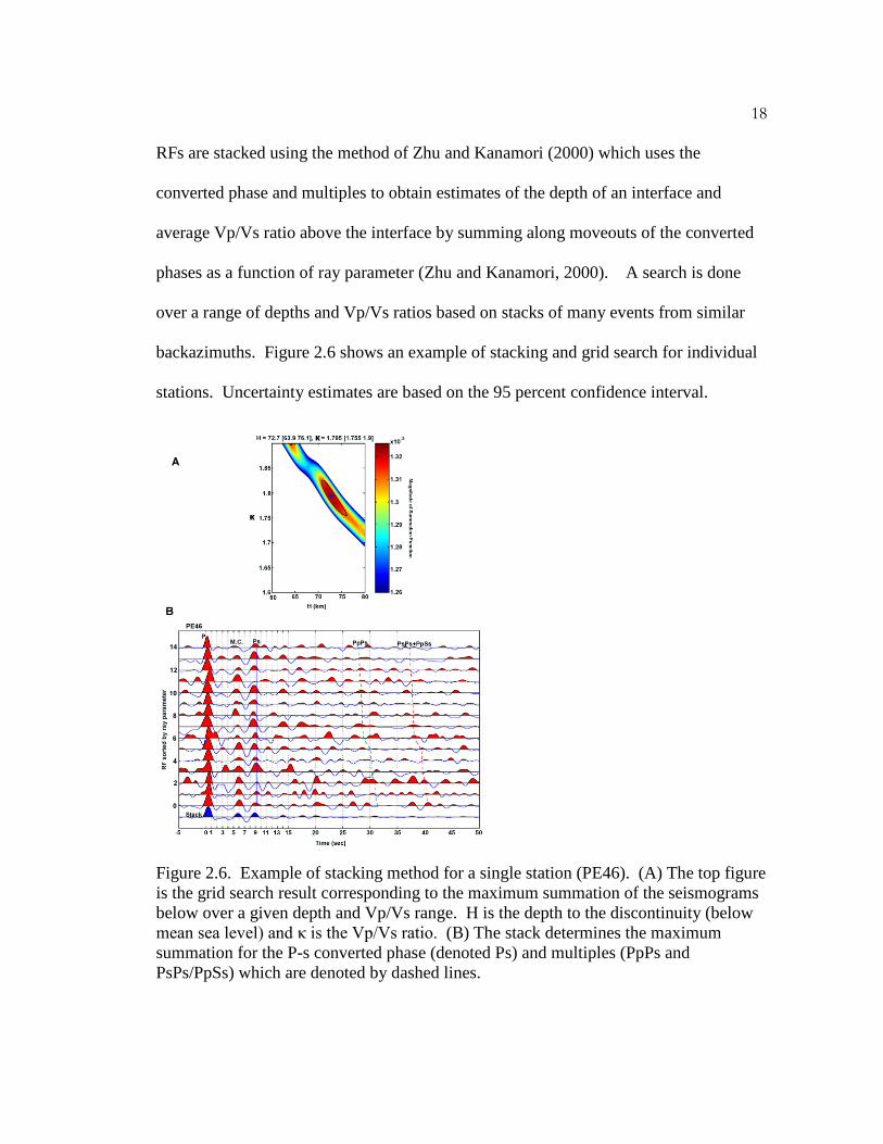
RFs are stacked using the method of Zhu and Kanamori (2000) which uses the

converted phase and multiples to obtain estimates of the depth of an interface and

average Vp/Vs ratio above the interface by summing along moveouts of the converted

phases as a function of ray parameter (Zhu and Kanamori, 2000). A search is done

over a range of depths and Vp/Vs ratios based on stacks of many events from similar

backazimuths. Figure 2.6 shows an example of stacking and grid search for individual

stations. Uncertainty estimates are based on the 95 percent confidence interval.

Figure 2.6. Example of stacking method for a single station (PE46). (A) The top figure is the grid search result corresponding to the maximum summation of the seismograms below over a given depth and Vp/Vs range. H is the depth to the discontinuity (below mean sea level) and κ is the Vp/Vs ratio. (B) The stack determines the maximum summation for the P-s converted phase (denoted Ps) and multiples (PpPs and PsPs/PpSs) which are denoted by dashed lines.

19

A simple migrated image is then constructed by backprojecting the receiver functions

along their ray paths. The angle from the station is estimated using the ray parameter

and event backazimuth, with corrections for the station elevation. A simple layered

velocity model based on IASP91 was used to backproject the rays. This approximation

was checked by comparison with other velocity models based on tomography and a

thicker crust but the migrated images were found to have Moho depths similar to the

results presented here.

2.2.1.1 Receiver Function Results

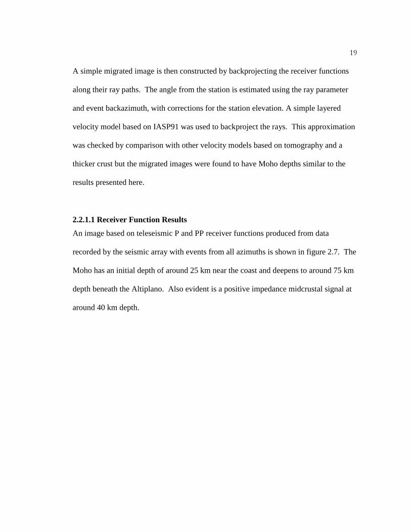
An image based on teleseismic P and PP receiver functions produced from data

recorded by the seismic array with events from all azimuths is shown in figure 2.7. The

Moho has an initial depth of around 25 km near the coast and deepens to around 75 km

depth beneath the Altiplano. Also evident is a positive impedance midcrustal signal at

around 40 km depth.

20

Figure 2.7. (A) Depth versus distance cross sectional image from Line 1 based on teleseismic P and PP receiver functions from all azimuthal directions showing the upper 120 km. Depth is the distance below mean sea level. (B) Same as in A showing interpretations of the mid crustal structure (MC) and Moho as well as a signal from the slab.

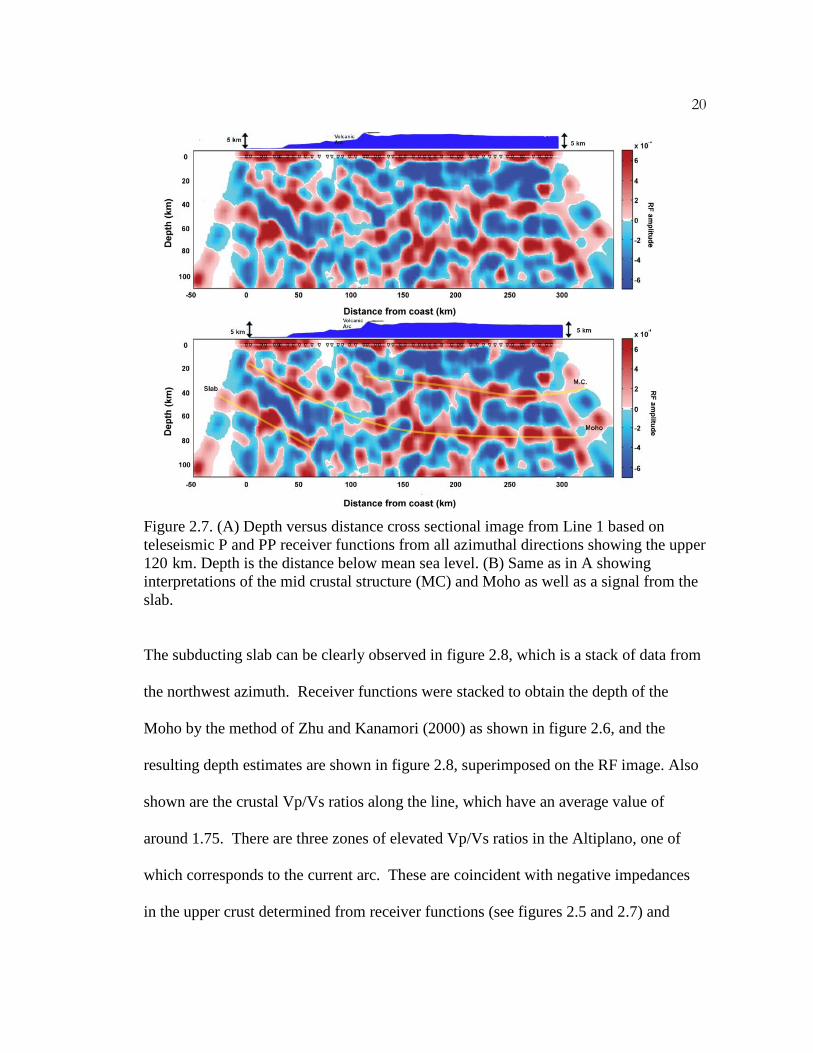
The subducting slab can be clearly observed in figure 2.8, which is a stack of data from

the northwest azimuth. Receiver functions were stacked to obtain the depth of the

Moho by the method of Zhu and Kanamori (2000) as shown in figure 2.6, and the

resulting depth estimates are shown in figure 2.8, superimposed on the RF image. Also

shown are the crustal Vp/Vs ratios along the line, which have an average value of

around 1.75. There are three zones of elevated Vp/Vs ratios in the Altiplano, one of

which corresponds to the current arc. These are coincident with negative impedances

in the upper crust determined from receiver functions (see figures 2.5 and 2.7) and

21

hence are likely related to magmatic processes. This identification is clearest for the

anomalies associated with the current arc. The other two may indicate the location of

focused magmatic activity in the past. Similar features were observed in northern Chile

(Leidig and Zandt, 2003; Zandt et al., 2003). The dense station spacing allows for an

unambiguous tracing of the Moho, slab, and midcrustal feature.

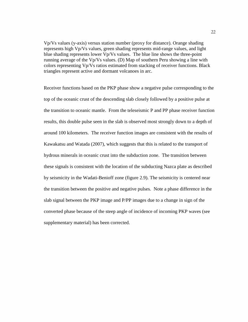
Figure 2.8. (A) Teleseismic P-wave Receiver function image based on events at a northwest azimuth to Peru with elevation along the array shown above. (B) Same image showing interpretation of the Moho, midcrustal structure, slab, and multiple of the midcrustal signal. Moho receiver function stacking results are plotted over the image. Elevation along the seismic line is shown above the image. (C) Average crustal

22

Vp/Vs values (y-axis) versus station number (proxy for distance). Orange shading represents high Vp/Vs values, green shading represents mid-range values, and light blue shading represents lower Vp/Vs values. The blue line shows the three-point running average of the Vp/Vs values. (D) Map of southern Peru showing a line with colors representing Vp/Vs ratios estimated from stacking of receiver functions. Black triangles represent active and dormant volcanoes in arc.

Receiver functions based on the PKP phase show a negative pulse corresponding to the

top of the oceanic crust of the descending slab closely followed by a positive pulse at

the transition to oceanic mantle. From the teleseismic P and PP phase receiver function

results, this double pulse seen in the slab is observed most strongly down to a depth of

around 100 kilometers. The receiver function images are consistent with the results of

Kawakatsu and Watada (2007), which suggests that this is related to the transport of

hydrous minerals in oceanic crust into the subduction zone. The transition between

these signals is consistent with the location of the subducting Nazca plate as described

by seismicity in the Wadati-Benioff zone (figure 2.9). The seismicity is centered near

the transition between the positive and negative pulses. Note a phase difference in the

slab signal between the PKP image and P/PP images due to a change in sign of the

converted phase because of the steep angle of incidence of incoming PKP waves (see

supplementary material) has been corrected.

23

Figure 2.9. Backprojected receiver function image based on PKP receiver functions. Only the PKPdf branch is included in this image. All events used come from the Indonesian region. Images show a sharp, well defined boundary at the expected location of the slab based on seismicity. Depth is the distance below mean sea level and distance is measured from the first station on the coast. Topography is shown above the image in blue.

2.2.1.2 Receiver Function Waveform Modeling

The receiver function images obtained above were checked using 2D finite-difference

waveform modeling (Kim et al. 2010). The 2D velocity model includes depth

information based on receiver function results and velocities consistent with averages

taken from Cunningham and Roecker (1986) for southern Peru, which we modified to

include a midcrustal layer contrast to model the positive-impedance feature. The more

recent model of Dorbath et al. (2008) was also tested and compared with the southern

Peru model (shown in the supplementary materials) and the results are similar to those

shown here. A simplified velocity model, which incorporates average values

consistent with these models for the crust, mantle wedge, subducting oceanic crust, and

24

underlying mantle was selected for modeling purposes. The model has dimensions of

500 km horizontal distance by 250 km depth. Synthetic receiver functions are produced

with P-wave plane waves with varying ray parameters imposed on the bottom and sides

of the model. Seismograms were produced with frequencies up to 1 Hz, and then

processed as RFs with the same techniques and parameters used with the real data. A

comparison of the synthetic and real receiver functions is shown in figure 2.10.

25

Figure 2.10. Velocity model and synthetic receiver functions obtained from finite difference modeling. To the right of the synthetics is an example of a receiver function and velocity model taken from the center of the model. A) Model with a homogenous crust, which recreates the Moho and slab signal as seen in receiver functions. B) Model that includes a midcrustal velocity jump recreates both the positive midcrustal signal seen at around 5 seconds and a multiple that also seen in the data. The signal from the Moho and slab are similar to the homogenous crustal model.

26

The synthetics, which incorporate midcrustal structure are observed to be consistent

with RF data and results as seen in figure 2.11. They show a positive signal at around 5

seconds (midcrustal), which is observed in the receiver functions as well as an observed

multiple that is not present in models without the midcrustal structure.

Figure 2.11. (A) Synthetic RF results from finite difference modeling are plotted over a sample receiver function from the magnitude 7.6 New Zealand earthquake on July 15, 2009 shown in figure 2.5. Green circles represent the midcrustal structure and orange

27

circles denote the depth of the Moho from synthetics. (B) Positive and negative pulses corresponding to the bottom and top of the oceanic crust of the slab as seen in FD synthetics are shown as magenta and yellow circles overlaying the PKP image from figure 2.10.

The velocity is then combined with a structural model derived from the receiver

functions and is tested with a deep local event that occurred beneath the array on the

slab interface (figure 2.12). The finite difference code is based on the one discussed in

Vidale et al. (1985). The event is Mb 6.0 and is located at a depth of 199 km and about

60 km off the line. The resultant synthetics from finite difference modeling have P

wave arrival characteristics and differential P to S wave travel times consistent with the

data. The synthetics and data also have a similar arrival caused by a conversion at the

Moho which provides confirmation of the Moho depth. An arrival due to phase

conversions at the midcrust can be seen in the synthetics and also appears to also be

present in the data, particularly towards the inland end of the seismic array suggesting

that the midcrustal structure does not underlie the entire seismic array in agreement

with receiver function observations.

28

Figure 2.12. Local waveform finite-difference modeling of local event near end of Line 1 A) Map showing event locations provided by National Earthquake Information Center (NEIC) and Instituto Geofisico del Peru (IGP). Also shown is the centroid moment tensor from the Harvard CMT database. B) Model used in the finite-difference

29

modeling. Shaded portions are extensions of the model to avoid artificial reflections. The location of the event at about 199km depth is shown by the pink circle. C) Data from a magnitude 6 event occurring on July 12, 2009 aligned by the P wave arrival (1). Time is on the x-axis and distance from coast is on the y-axis. D) Synthetics also aligned on the P wave arrival (1). The S wave arrival (2) can also be seen as well as signals from the Moho (3) and midcrustal interface (4). E) Comparison of data and synthetics near the P wave arrival where the synthetics are in red and the data is shown by the black line.

2.2.2 P-Wave Tomography

A total of 5677 travel–time residuals including 1674 teleseismic arrivals and 4003

local event arrivals were inverted to obtain the tomographic image shown in figure 2.13

using a 2D tomography program (Husker and Davis, 2009). The local events are

restricted to depths greater than 30 km, and with 125 km of the 2D line. The 2D

assumption appears justified by gravity based on gravity survey results (Fukao et al.

1989) and GRACE (Gravity Recovery and Climate Experiment) satellite data which

show little along-strike gravity variation indicating an approximately 2D crust, as well

as seismicity slab contours which show that the slab can also be considered

approximately 2D within about 100km of the array. The local earthquakes were first

located with an IASPEI (Kennett and Engdahl 1991) model that took into account the

changing Moho depth determined by receiver functions. A finite-difference program

was then used to relocate the events (Hole and Zeldt, 1995). The inversion consisted

of 680 20 km blocks (20x34) and was performed with damped least squares. In the

upper 350 km; the average number of hits/block was 142. The variance reduction was

88%. The final image was smoothed with a 2x2 block running average.

30

Figure 2.13. Tomographic image beneath the seismic line using a 2D tomography code. In A) the results are percent slowness changes from the IASPEI model, and in B) the result is in absolute velocity. Locations of the Moho and top of the Slab from the receiver function study are plotted as white lines. Station locations are shown as black triangles and local earthquake locations used for tomography are shown as black circles. The image supports the model of a steeply dipping slab and thickened Moho.

The tomography results are presented in figure 2.13. Figure 2.13A shows perturbations

as percent deviations relative to the IASPEI starting model while figure 2.13B shows

the absolute P wave velocity. The cross section chosen lies along a straight line

31

through the station locations. For comparison, locations of the Moho and top of the

subducting slab from the receiver function analysis are superimposed on the figure and

show good agreement with the transitions in the image from low to higher velocities.

A standard checkerboard resolution test is shown in figure 2.14. The results are well

resolved in both the horizontal and vertical directions except at depth greater than 350

km on the northern end of the line.

Figure 2.14. Tomographic resolution test. The results of a standard checkerboard resolution test are shown corresponding to the tomographic depth cross section for the array. Depth in kilometers is shown on the y-axis and distance in kilometers on the x-axis. A) The upper figure shows the checkerboard input model. B) The lower figure shows the output based on event coverage.

32

2.3 Discussion

2.3.1 Crustal Thickness

Receiver function results for the normal subducting region of southern Peru show a

Moho that deepens from 25 km near the coast to a depth of around 75 km beneath the

Altiplano. Previous estimates of crustal thickness of the Altiplano are about 70-75 km

(Cunningham and Roeker, 1986; Beck et al., 1996; Zandt et al, 1994). McGlashan et al.

(2008) also estimated thicknesses from 59 to 70 in Southern Peru. The 75 km crust of

the Altiplano is approximately the thickness required for the region to be in Airy

isostatic equilibrium and this is verified with the gravity observations (figure 2.15).

33

Figure 2.15. Results from a gravity survey performed along the seismic array by Caltech and UCLA students during a geophysical field course. A) Observed absolute gravity (m/s2) B) Free air anomaly in mGal relative to the first station, which shows an increase near the start of the line due to uplift near the coast. (C) Topography along the array (D) Moho estimates from receiver function stacking and Moho depth estimates expected for Airy isostasy relative to a reference station.

One of the major processes which could contribute to this thickness is crustal

shortening. Gotberg et al. (2010) gave a preferred estimate of 123 km of shortening but

said that 240-300 km of shortening would be required for a 70 km thick crust. Other

suggested mechanisms for producing such a thickness include lower-crustal flow,

shortening hidden by the volcanic arc (Gotberg et al., 2010), thermal weakening

(Isacks, 1988; Allmendinger et al., 1997; Lamb and Hoke, 1997), regional variation in

34

structure from tectonic events prior to orogeny (Allmendinger and Gubbels, 1996),

magmatic additions, lithospheric thinning, upper mantle hydration (Allmendinger et al.,

1997), plate kinematics (Oncken et al., 2006), shortening related to the Arica bend

(Kley & Monaldi, 1998; Gotberg et al, 2010), tectonic underplating (Allmendinger et

al, 1997; Kley & Monaldi, 1998), and other factors. The mechanism of tectonic

underthrusting is supported by our observations of a midcrustal structure and provides a

simple mechanism for explaining the crustal thickness in southern Peru.

2.3.2 Midcrustal Structure

The positive impedance structure observable at a depth of around 40 km is an unusual

crustal feature because the crust does not normally have an interface with a sharp

increase in velocity. One hypothesis that could explain this feature is underthrusting by

the Brazilian Craton. It is generally accepted that this underthrusting exists as far as the

Eastern Cordillera (McQuarrie et al., 2005; Gubbels et al., 1993; Lamb & Hoke, 1997;

Beck & Zandt, 2002). However the results presented here appear to support the idea

that it extends further to the west, as was suggested by Lamb and Hoke (1997). The

midcrustal signal at 40 km depth is observed continuously across multiple stations on

the eastern half of the array. The Conrad discontinuity, which is sometimes observed at

midcrustal depths of around 20 km was considered, but the processes involved in

crustal shortening and thickening are not expected to produce such a flat and strong

positive impedance feature at 40 km. The strength of the midcrustal signal relative to

the Moho signal (see figure 2.6), and the observation that the signal is limited to the

easternmost stations in the array rather than across the whole array support

35

underthrusting as a more reasonable explanation. If the Brazilian craton underthrusts as

far as the Altiplano, it would substantially increase the thickness of the crust under the

Altiplano and hence affect the timing of the rise of the Andes. The rapid rise model of

Garzione et al. (2008), proposes a gradual rise of 2 km over approximately 30 Myrs,

followed by a rapid rise of 2 km over the last 10 Myrs. This is then used as evidence of

removal of the dense lower crust and/or lithospheric mantle (Ghosh et al. 2006) because

it is a process that can result in rapid uplift. An alternative model of the rise suggests

that the total rise proceeded gradually over 40 Myrs. This latter model is favored by the

midcrustal layer found in this study. The timing of underthrusting and nature of the

underthrusting Brazilian craton suggests that rather than eclogitization and

delamination of the lower crust and mantle lithosphere resulting in rapid uplift, the

process was more gradual. The underthrusting Brazilian craton would have removed

some of the preexisting lower crust and mantle lithosphere beneath the Altiplano and

replaced it with the Shield crust and underlying mantle lithosphere, thus contributing to

the crustal thickening observed beneath the Altiplano. Some of the uppermost crust of

the underthrusting Brazilian craton may have been eroded and deformed. The

remainder of the Shield crust is assumed to be denser than the upper Altiplano crust

resulting in higher seismic velocities. The lithosphere of the Brazilian craton is

suggested to taper off prior to the subducting Nazca plate as the subducting plate is

observed continuously to 250 km depth and is not impacted by the underthrusting

craton. The western limit of the underthrusting is not well defined in the images but it

does not appear to extend beyond the volcanic arc. The presence of the underthrusting

material is not expected to interfere with processes or arc magmatism.

36

Comparing the model of evolution in Southern Peru with the overall evolution in the

central Andes, several authors (Allmendinger et al., 1997; Babeyko and Sobolev, 2005)

have suggested that there has been north–south variation in mechanisms and rates of

crustal thickening and uplift in the central Andes. The tectonic evolution in the

Altiplano may have differed from the uplift and evolution of the Puna plateau

(Allmendinger et al, 1997). Babeyko and Sobolov (2005) suggested that the type of

shortening (e.g., pure versus simple shear as discussed by Allmendinger and Gubbels,

1996) may be controlled by the strength of the foreland uppermost crust and

temperature of the foreland lithosphere. Hence, a weak crust and cool lithosphere in

the Altiplano could be supportive of underthrusting, simple shear shortening, and

gradual uplift while further south in the Puna the strong sediments and warm

lithosphere supports pure shear shortening, lithospheric delamination, and resultant

rapid uplift.

In addition to crustal information, receiver functions also show the subducting Nazca

plate dipping at an angle of about 30 degrees from both the P/PP and PKP phases for

Line 1. Figure 2.16 shows a cartoon interpretation of the array data. With the exception

of the midcrustal positive-impedance and its interpretation of underthrusting by the

Brazil Craton, the subduction appears to be normal.

37

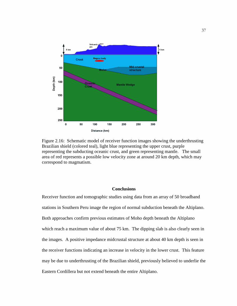
Figure 2.16: Schematic model of receiver function images showing the underthrusting Brazilian shield (colored teal), light blue representing the upper crust, purple representing the subducting oceanic crust, and green representing mantle. The small area of red represents a possible low velocity zone at around 20 km depth, which may correspond to magmatism.

Conclusions

Receiver function and tomographic studies using data from an array of 50 broadband

stations in Southern Peru image the region of normal subduction beneath the Altiplano.

Both approaches confirm previous estimates of Moho depth beneath the Altiplano

which reach a maximum value of about 75 km. The dipping slab is also clearly seen in

the images. A positive impedance midcrustal structure at about 40 km depth is seen in

the receiver functions indicating an increase in velocity in the lower crust. This feature

may be due to underthrusting of the Brazilian shield, previously believed to underlie the

Eastern Cordillera but not extend beneath the entire Altiplano.

38

Acknowledgements

We thank the Betty and Gordon Moore Foundation for their support through the

Tectonics Observatory at Caltech. This research was partially support by NSF award

EAR-1045683. Contribution number 199 from the Tectonics Observatory at Caltech.

Chapter 2 References

∙ Ahrens, T. J., and G. Schubert (1975). Gabbro-Eclogite reaction rate and its

geophysical significance, Reviews of Geophysics and Space Physics, 13 (2), 383-400

∙ Allmendinger, R., and T. Gubbels (1996), Pure and simple shear plateau uplift,

Altiplano-Puna, Argentina and Bolivia, Tectonophysics, 259, 1–13.

∙ Allmendinger, R., T. Jordan, S. Kay, and B. Isacks (1997), The e volution of the

Altiplano-Puna Plateau of the Central Andes, Annu. Rev. Earth Planet. Sci., 25,

139–174.

∙ Ammon, C., (1991), The isolation of receiver effects from teleseismic P waveforms,

Bull. Seismo. Soc. Am., 81, 6, 2504-2510.

∙ Babeyko, A., and S. Sobolev (2005), Quantifying different modes of the late

Cenozoic shortening in the central Andes, Geology, 33 (8), 621–624.

∙ Barazangi, M., and B. L. Isacks (1976), Spatial distribution of earthquakes and

subduction of the Nazca plate beneath South America, Geology, 4, 686–692.

∙ Barnes, J., and T. Ehlers (2009), End member models for Andean Plateau uplift,

Earth-Science Reviews, 97 (105-132).

∙ Beck, S., and G. Zandt (2002), The nature of orogenic crust in the Central Andes,

J. of Geophys. Res., 107, 2230.

39

∙ Beck, S., G. Zandt, S. Myers, T. Wallace, P. Silver, and L. Drake (1996), Crustal-

thickness variations in the central Andes, Geology, 24 (5), 407–410.

∙ Cunningham, P., and S. Roecker (1986), Three-dimensional P and S Wave Velocity

Structures of Southern Peru and Their Tectonic Implications, J. of Geophys.

Res., 91 (B9), 9517–9532.

∙ DeCelles, P., and M. Ducea, P. Kapp and G. Zandt (2009), Cyclicity in Cordilleran

orogenic systems, Nature Geoscience, 2, pp 251-257, doi:10.1038/NGEO469.

∙ Dorbath, C., M. Gerbault, G. Carlier, and M. Guiraud (2008), Double seismic zone of

the Nazca plate in Northern Chile: High-resolution velocity structure, petrological

implications, and thermomechanical modeling, Geochemistry, Geophysics,

Geosystems, 9 (7), Q07, 2006.

∙ Ehlers, T., and C. Poulsen (2009), Influence of Andean uplift on climate and

paleoaltimetry estimates, Earth and Planetary Science Letters, 281, 238–248.

∙ Elger, K., O. Oncken, and J. Glodny (2005), Plateau-style accumulation of

deformation: Southern Altiplano, Tectonics, 24 (TC4020).

∙ Engdahl, E. R., R. van der Hilst, and R. Buland (1998), Global teleseismic earthquake

relocation with improved travel times and procedures for depth determination, Bull.

Seism. Soc. Am. 88, 722-743

∙ Engdahl, E. R. and A. Villaseñor (2002), Global Seismicity: 1900-1999, in W.H.K.

Lee, H. Kanamori, P. C. Jennings, and C. Kisslinger (editors), International

Handbook of Earthquake and Engineering Seismology, Part A, Chapter 41, 665-690

∙ Fukao, Y., A. Yamamoto, and M. Kono (1989), Gravity anomaly across the Peruvian

Andes, Journal of Geophysical Research, 94, (B4)

40

∙ Garzione, C., P. Molnar, J. Libarkin, and B. MacFadden (2006), Rapid late Miocene

rise of the Bolivian Altiplano: Evidence for removal of mantle lithosphere, Earth

and Planetary Science Letters, 241, 543–556.

∙ Garzione, C., G. Hoke, J. Libarkin, S. Withers, B. MacFadden, J. Eiler, P. Ghosh, and

A. Mulch (2008), Rise of the Andes, Science, 320, 1304–1307.

∙ Ghosh, P., C. Garzione, and J. Eiler (2006), Rapid uplift of the Altiplano revealed

through 13C-18O bonds in paleosol carbonates, Science, 311, 511–515.

∙ Gotberg, N., N. McQuarrie, and V. Caillaux (2010), Comparison of crustal thickening

budget and shortening estimates in southern Peru (12˚–14˚ S): Implications for

mass balance and rotations in the “Bolivian orocline”, GSA Bulletin, 122 (5–6), 727–

742.

∙ Gregory-Wodzicki, K. (2000), Uplift history of the Central and Northern Andes; a

review, GSA Bulletin, 112 (7), 1091–1105.

∙ Gubbels, T., B. Isacks, and E. Farrar (1993), High-level surfaces, plateau uplift, and

foreland development, Bolivian central Andes, Geology, 21, 695–698.

∙ Gutscher, M., W. Spakman, H. Bijwaard, and E. Engdahl (2000), Geodynamics of flat

subduction: Seismicity and tomographic constraints from the Andean margin,

Tectonics, 19 (5), 814–833.

∙ Hacker, B.R. (1996), Eclogite formation and the rheology, buoyancy, seismicity, and

H2O content of oceanic crust, AGU Monograph, p337-346.

∙ Hampel, A. (2002), The migration history of the Nazca Ridge along the Peruvian

active margin: a re-evaluation, Earth and Planetary Science Letters, 203, 665–679.

∙ Hole, J. A., and B. C. Zelt (1995), 3-D finite-difference reflection traveltimes,

41

Geophys. J. Int., 121, 427-434.

∙ Horton, B., B. Hampton, and G. Waanders (2001), Paleogene synorogenic

sedimentation in the Altiplano Plateau and implications for initial mountain building

in the Central Andes, GSA Bulletin, 113, 1387–1400.

∙ Husker, A. and P. M. Davis (2009), Tomography and thermal state of the Cocos

plate subduction beneath Mexico City, J. Geophys. Res., 114, B04306.

∙ Isacks, B. (1988), Uplift of the Central Andean Plateau and bending of the Bolivian

Orocline, J. of Geophys. Res., 93 (B4), 3211–3231.

∙ Kawakatsu, H., and S. Watada (2007), Seismic evidence for deep-water

transportation in the mantle, Science, 316, 1468-1471.

∙ Kennett, B. L. N., and E. R. Engdahl (1991), Traveltimes for global earthquake

location and phase identification, Geophys. J. Int., 105, 429-465.

∙ Kim, Y., R. W. Clayton, and J. M. Jackson (2010), Geometry and seismic properties

of the subducting Cocos plate in central Mexico, J. Geophys. Res., 115, B06310.

∙ Kley, J. and C. R. Monaldi (1998), Tectonic shortening and crustal thickness in the

Central Andes: How good is the correlation? , Geology, 26, 8, 723-726.

∙ Lamb, S., and L. Hoke (1997), Origin of the high plateau in the Central Andes,

Bolivia, South America, Tectonics, 16 (4), 623–649.

∙ Langston, C. (1979), Structure under Mount Rainier, Washington, inferred from

teleseismic body waves, J. Geophys. Res., 84, 4749–4762.

∙ Leidig, M., and G. Zandt (2003), Modeling of highly anosotropic crust and application

to the Altiplano-Puna volcanic complex of the central Andes, J. Geophys. Res, 108

(B1).

42

∙ McGlashan, M., L. Brown, and S. Kay (2008), Crustal thickness in the Central Andes

from teleseismically recorded depth phase precursors, Geophys. J. Int., 175, 1013-

1022.

∙ McQuarrie, N., B. Horton, G. Zandt, S. Beck, and P. DeCelles (2005), Lithospheric

evolution of the Andean fold-thrust belt, Bolivia, and the origin of the central

Andean plateau, Tectonophysics, 399, 15–37.

∙ Norabuena, E., J. Snoke, and D. James (1994), Structure of the subducting Nazca

Plate beneath Peru, J. Geophys. Res., 99, 9215–9226.

∙ Oncken, O., J. Kley, K. Elger, P. Victor, and K. Schemmann (2006), Deformation of

the Central Andean Upper Plate System-Facts, Fiction, and Constraints for Plateau

Models, Berlin, Springer, p. 569.

∙ Ramos, V. (2009), Anatomy and global context of the Andes: Main geologic features

and the Andean orogenic cycle, in Kay, S.M., Ramos, V.A., and Dickinson, W.R.,

eds., Backbone of the Americas: Shallow Subduction, Plateau Uplift, and Ridge and

Terrane Collision: Geological Society of America Memoir, 204, p31065,doi:

10.1139/2009.1204(02).

∙ Sighinolfi, G.P. (1971), Investigations into deep crustal levels: fractionating effects

and geochemical trends to high-grade metamorphism, Geochim. Cosmochim. Acta,

35, pp. 1005-1021.

∙ Tassara, A. (2006), Factors controlling the crustal density structure underneath active

continental margins with implications for their evolution, Geochem. Geophys,

Geosyst., 8, Q01001.

∙ Vidale, J., D. Helmberger, and R. Clayton, (1985), Finite-difference synthetic

43

seismograms for SH-waves, Bull. Seismo. Soc. Am., 75, 6, 1765-1782.

∙ Yan, Z. and R.W. Clayton (2007), Regional mapping of the crustal structure in

southern California from receiver functions, J. of Geophys. Res., 112, B05311.

∙ Zandt, G., M. Leidig, J. Chmielowski, D. Baumont, and X. Yuan (2003), Seismic

detection and characterization of the Altiplano-Puna magma body, Central Andes,

Pure Appl. Geophys., 160, 789–807.

∙ Zandt, G., A. Velasco, and S. Beck (1994), Composition and thickness of the southern

Altiplano crust, Bolivia, Geology, 22, 1003–1006.

∙ Zhu, L., and H. Kanamori (2000), Moho depth variation in southern California from

teleseismic receiver functions, J. Geophys. Res., 105 (B2), 2969–2980.