Chapter 2 Instrumental and Experimental Methods - … · Chapter 2 Instrumental and Experimental Methods . ... Conversion of force curves . ... (Albrecht . et al. 1990; Butt

Chapter 2 Methods

Chapter 2 Instrumental and Experimental

Methods

Atomic force microscopy (AFM) is a powerful tool to investigate the

morphology and mechanical properties of protein nanotubes. In this chapter, the

principles of AFM will be first introduced. Then the protocols of AFM analysis

and image processing used in the later chapters will be explained. The preparation

of protein nanotube samples for AFM analysis will also be presented.

2.1 Atomic Force Microscopy

2.1.1 Atomic Force Microscopy

AFM, which was invented in 1986, expanded the application of scanning

tunnelling microscopy to nonconductive, soft, and live biological samples (Binnig

et al. 1986; Zasadzinski et al. 1998; Marti et al., 1998). AFM has several

capabilities including the ability to characterize topographic details of surfaces

from the submolecular to the cellular level (Radmacher et al. 1992), monitor the

dynamic processes of single molecules in physiologically relevant solutions

(Engell and Muller 2000), and measure the forces between interacting molecules

(Zlatanova et al. 2000). AFM is a powerful tool for characterizing the structural

properties of macromolecular complexes both in air and under near-physiological

conditions. In addition, modified AFMs can be used to manipulate single

44

Chapter 2 Methods

molecules (Yang et al. 2003). In the past two decades, the application of AFM has

spread to many areas of biological sciences including studies of DNA (Fritzsche

et al. 1997; Hansma 2001), RNA (Lyubchenko et al.1992; Bonin et al. 2000;

Henn et al. 2001; Liphardt et al. 2001), proteins (Heymann et al. 1997; Isralewitz

et al. 2001), lipids (Dufrene 2000; Balashev et al. 2001), carbohydrates (Misevic

1999; Dettmann et al. 2000; Marszalek et al. 2001), biomolecular complexes

(Lyubchenko et al. 1995; Willemsen et al. 2000; Safinya 2001), organelles

(Oberleithner et al., 1997; Danker and Oberleithner 2000) and cells (Henderson

1994; Ohnesorge et al. 1997).

2.1.1.1 Principle of AFM

The principle of the AFM is relatively simple (Figure 2-1). The key element of

the AFM is the cantilever. It consists of one or more beams of silicon or silicon

nitride of 100–500 μm in length and 0.5–5 μm in thickness. At the end of the

cantilever a sharp tip is mounted to sense the force acting between it and the

sample surface. Photos of general purpose silicon nitride cantilevers (Veeco

Probes, Camarillo, CA, USA) are shown in Figure 2-2. For normal topographic

imaging, the tip is brought into continuous or intermittent contact with the sample

as it raster-scans over the surface. An optical system is then used to measure the

changes of the laser beam reflected from the gold-coated back of the cantilever

onto a position-sensitive photodiode (PSPD), which can measure changes in the

position of the incident laser as small as 0.1 nm.

45

Chapter 2 Methods

Figure 2-1 Schematic of the concept of AFM and the optical lever.

Figure 2-2 Photos of a general purpose silicon nitride cantilever produced by Veeco Probes.

Two cantilevers with the tips pointing upwards are shown on the left. A tip is shown on the

right. The tip height is 2.5-3.5 μm, the thickness of the cantilever is 0.4-0.7 μm. The triangular

cantilever lengths are 196 μm and 115 μm respectively.

<URL: https://www.veecoprobes.com/probe_detail.asp?ClassID=17> [Accessed 22 Feb 2008]

46

Chapter 2 Methods

2.1.1.2 Operation Modes of AFM

The AFM is available in several operating modes, including contact mode and

tapping mode, which are chosen depending on the sample, environment, and

measurements required.

In contact mode (CM), the AFM cantilever is deflected by the sample surface

(Yang et al., 2003). Generally, the cantilever deflection is kept constant by the use

of a piezoelectric feedback system which permanently regulates the vertical (z)

position of either the tip or the sample and produces a constant force image

(Bonnell 2001). The image represents the topographic structure of the surface.

Deflection is not the most sensitive measurement, having a relatively small signal-

to-noise ratio. Furthermore, due to direct contact with the sample, the scanning

motion induces lateral forces onto the material which can be intolerable for soft

surfaces. However, in some cases, contact mode is still the imaging mode of

choice. For example, the alternative modes do not provide the direct information

of the force applied onto the sample surface by the tip (Salvetat 1999).

Tapping mode (TM) uses an alternative and more sensitive measurement: the

vibrational characteristics of the cantilever. The mechanical resonant frequency of

the cantilever is determined by the dimensions of the structure and the properties

of materials from which it is made. The vibration amplitude detected at a given

frequency changes as a function of the force gradient. Varying the vertical

position of the tip such that the amplitude of oscillation at a particular frequency is

constant produces a constant force gradient image. TM has a larger signal-to-noise

ratio than does CM (Bonnell 2001). It also generates smaller lateral forces on the

sample, which improves the lateral resolution of the AFM image, as well as

47

Chapter 2 Methods

reducing the damage to the sample while scanning. Consequently, TM is often

preferred over CM for most biological applications (Yang et al., 2003).

Phase imaging is relatively new and has the advantage of being able to be

performed at the same time as topographic imaging with tapping mode, i.e. both

topographic and phase images can be obtained in a single scan. Because the

interactions between the tip and the surface depend not only on the topography of

the sample but also on other characteristics (such as hardness, elasticity, adhesion,

or friction), the movements of the cantilever to which the tip is attached depend

also on these properties. In phase imaging, the phase of the sinusoidal oscillation

of the cantilever is measured relative to the driving signal applied to the cantilever

to cause the oscillation. Phase images are produced by recording this phase shift

during the tapping mode scan. Phase imaging can detect, for example, different

components in polymers related to their stiffness or areas of different

hydrophobicity in hydrogels immersed in saline solutions (Magonov and Reneker

1997).

2.1.1.3 Force Measurements by AFM

In addition to imaging AFM can also probe elastic properties or adhesion on a

surface by generating force curves. These curves are generated by performing

controlled vertical tip-sample interactions, without lateral scanning movement and

while recording the cantilever’s deflections. Force curves measure nano- to pico-

Newton range vertical forces applied to the surface, and allow the estimation of

the nanomechanical properties of the samples. The ability to coat the tip with

different molecules (proteins, lipids) has increased the utility of force curves in

understanding the specific attraction between a ligand and its receptor (Dammer et

48

Chapter 2 Methods

al. 1996; Vinckier et al. 1998). This technique can also be used to measure charge

densities on surfaces (Heinz and Hoh 1999), to estimate the folding force of

biomolecules like titin (Rief et al. 1997), and to measure forces associated with

polymer elongation (Rief et al. 1998).

Conversion of force curves

The direct result of a force measurement is a curve of the photodiode current I

versus height position of the piezoelectric translator ZP. In order to obtain the

curve of tip-sample interactive force F versus piezo displacement ZP, the I signal

must be converted to F. This is explained as follows by an ideal example as in

Figure 2-3, which is a model curve as would be observed for an infinitely hard

sample surfaces with no surface forces. The curves of the tip approaching to and

retracting from the surface are identical. The horizontal part (Figure 2-3 A-B) is

the non-contact line. The linearly increasing part (Figure 2-3 B-C) is the contact

line, from the slope of which the sensitivity ΔI/ΔZP can be obtained. The I signal

can be converted into a cantilever deflection Zc by dividing the I signal by the

sensitivity, which leads to Zc = I/(ΔI/ΔZP). Knowing the spring constant of the

cantilever kc, the I signal can easily be converted into force according to Hooke’s

Law: F = kcZc. The non-contact line defines zero deflection of the cantilever,

which is therefore the zero force line (Butt et al. 2005).

49

Chapter 2 Methods

Figure 2-3 A model force measurement curve recorded for an infinitely hard material surface

with no surface forces. The approaching and retracting curves are identical. The I vs. ZP curve

is converted to F vs. δ curve. A-B is the non-contact line and B-C is the contact line.

Problem of zero tip-sample distance

The true tip-sample distance, or the indentation δ is the piezo displacement ZP

deduced by the cantilever deflection Zc: δ = ZP - Zc. Using the ideal example of an

infinitely hard sample surface without surface forces again (Figure 2-3), the

definition of zero indentation is as follows: The zero cantilever deflection Zc0 lies

on the horizontal non-contact line (Figure 2-3 A-B). The point where the two linear

50

Chapter 2 Methods

parts of the force curve cross is defined as zero piezo displacement ZP0 (Figure 2-3

B). The curve of force F versus piezo displacement ZP then can be converted to

force F versus indentation δ (= (ZP - ZP0) - (Zc - Zc0)) curve.

Figure 2-4 A force measurement retracting curve for a deformable material with attraction

and adhesion forces. The I vs. ZP curve is converted to F vs. δ curve.

However, in reality, especially for biological samples, the definition of zero

indentation is more complicated. A typical retracting force curve of deformable

materials with surface forces is displayed in Figure 2-4. Note that for deformable

materials, the approach and retract curves of a force measurement are no longer

51

Chapter 2 Methods

identical. The approach curve is used to define zero tip-sample distance. The zero

cantilever deflection lies on the horizontal non-contact line at large distances away

from the surface, where surface forces are negligible. The sensitivity is obtained

from the linear contact part of the approach curve. One way to find the zero piezo

displacement ZP0 is to extrapolate the two linear regimes of the approach curve.

Another way to find ZP0, which is more robust and reliable, is to fit experimental

data in the range on the approach curve when the tip and sample are in contact

using a Hertzian model as described in Equation 2-1 (Hertz 1882; Rotsch et al.

1999; Bhanu and Hörber 2002).

20

0 0( )(1( )

(2 / ) tan( )c c c

P P c ck Z ZZ Z Z Z

E)υ

π α⋅ − −

− = − +⋅ ⋅

Equation 2-1

where kc is the spring constant; α is the half-opening angle of a conical shaped tip;

ν is the Poisson ratio and E is the elastic modulus. E and ZP0 are two unknown

variables, which are determined by the fit. By employing a Monte Carlo fit, it is

possible to optimize values of E and ZP0. Igor software (Igor Pro version 4;

WaveMetrics, OR, USA) was used to perform this type of fitting in chapter 5 of

this thesis.

Determination of spring constant of the cantilever

For AFM force measurements, the value of spring constant of the cantilever is

usually needed. Several methods have been described, but many do not appear to

be simple, reliable and precise at the same time (Albrecht et al. 1990; Butt et al.

1993; Neumeister and Ducker 1994; Sader 1995; Sader et al. 1995, 1999; Senden

and Ducker 1994; Cleveland et al. 1993; Gibson et al. 1996).

52

Chapter 2 Methods

Hutter and Bechhofer (1993) proposed an elegant and widely used method,

which is implemented in many commercial AFMs. They suggested to measure the

intensity of the thermally excited cantilever oscillations or the cantilever thermal

noise. For an ideal spring of spring constant kc, the mean square deflection of the

cantilever is:

2 Bc

c

k TZk

=

Equation 2-2

where kB is the Boltzmann constant and T is the absolute temperature.

In reality, considering the shape of the cantilever (which leads to several

possible vibration modes) (Butt and Jaschke 1995) and the systematic error of the

deflection detecting technique (usually optical lever technique) (Stark et al. 2001),

there is:

**2

Bc

k TkZ

β=

Equation 2-3

where Z* is the effective deflection, which is the deflection read from the

instrument after determining the sensitivity from the contact part of a force curve

on a hard substrate; β* is the effective correction factor, which is 0.817 for a

rectangular cantilever and 0.764 for a V-shape cantilever (Stark et al. 2001).

In practice, a force curve is acquired on a hard substrate to characterize the

sensitivity, and then a noise spectrum of the deflection amplitude is taken. This

spectrum shows a peak at the resonance frequency. The peak is fitted with a

Lorentzian curve and the mean square deflection of the peak is obtained by

53

Chapter 2 Methods

integration. The thermal noise method was used to obtain the spring constant of

cantilever in chapters 5 and 6 of this thesis.

2.1.2 AFM Analysis

AFM Imaging

AFM imaging experiments presented in section 3.1, 3.2, 4.2, 4.3 and 6.2 were

carried out using MultiMode scanning probe microscope with Nanoscope IIIa

controller (Veeco, Metrology Group, Santa Barbara, CA, USA) equipped with an

E-scanner (maximum scan size 10 µm × 10 µm, vertical range 2.5 µm). AFM

imaging experiments presented in section 3.3, 4.4 and 6.3.1 were carried out using

the same MultiMode AFM equipped with a J-scanner (maximum scan size 125

µm × 125 µm, vertical range 5.0 µm).

For the AFM imaging experiments presented in section 6.3.2 and 6.3.3, an

EnviroScope AFM (eScope AFM; Digital Instruments) was used. This AFM has

an enclosed sample chamber allowing the control of temperature (from room

temperature up to 185ºC in air) and humidity (range of 0-80% RH).

Silicon probes (OMCL-AC160TS, Olympus Optical, Tokyo, Japan) with

nominal spring constant 34.4~74.2 N/m were used for images obtained using

tapping mode in air. V-shaped silicon nitride levers (Veeco Probes, Camarillo, CA,

USA) with a nominal spring constant of 0.32 N/m were used for images obtained

using tapping mode in liquid. The V-shaped silicon nitride levers (Veeco Probes)

with nominal spring constants of 0.06 N/m were used for contact mode in air

(these are all manufacturer’s data). Scan rates employed were typically 1.0-2.0 Hz.

54

Chapter 2 Methods

AFM force measurements

Force measurements presented in chapter 5 were carried out using MultiMode

AFM equipped with a Picoforce module (Digital Instruments). V-shaped silicon

nitride levers (Veeco Metrology Group) with nominal spring constants of 0.06

N/m (manufacturer’s data) were used for force measurements.

2.1.3 Image Processing

AFM image data were analyzed with SPIP software (The Scanning Probe Image

Processor, Version 3.3.9.0; Image Metrology A/S, Denmark). It should be noted

that, in this thesis, the “height” of a sample means the vertical difference between

the top of the sample and the substrate surface; while the “width at the half

height” means the horizontal width of a sample at the half of the height of the

sample. It is demonstrated in Figure 2-5 how the height and the half height width

of a diphenylamine nanotube from an AFM height image were determined using

SPIP software.

55

Chapter 2 Methods

Figure 2-5 Measurement of the dimensions of a protein nanotube from an AFM height image

using SPIP. The left picture is an AFM height image of a diphenylalanine nanotube on silicon

grid substrate with square holes of 5 μm × 5 μm. The two pictures on the right are the profiles

along the white line (which is perpendicular to the direction of the nanotube of interest) on the

left image. The vertical difference between the tips of the two pink triangles on the top right

profile is the “height” of the nanotube. The horizontal difference between the tips of the two

green triangles on the bottom right profile is the “width at the half height”.

2.2 Preparation of Protein Nanotubes

2.2.1 Bacterial Flagellar Filaments

Salmonella flagellar filaments were removed from cells by mechanical shearing.

Deflagellated cells were removed by centrifugation, and then the flagellar

filaments were collected by ultracentrifugation. Salmonella flagellar filament

samples were stored in 10mM HEPES (pH 7.0, pKa 7.31) and were kindly

56

Chapter 2 Methods

provided by Dr. Richard Woods from Queen’s Medical Centre (QMC), University

of Nottingham.

2.2.2 Lysozyme Fibrils

Chicken egg-white lysozyme (dialyzed lyophilized powder; Sigma Chemical

Company, St. Louis, MO, USA) was dissolved to 10mg/mL in 10mM glycine

(C2H5NO2; SigmaUltra; Sigma Chemical Company) buffer (pH 2.0). Then

lysozyme solution was incubated in an electrical oven at 57 ± 2 °C (Krebs, et al.

2000).

2.2.3 β2-Microglobulin Fibrils

β2-microglobulin (lyophilized powder; Sigma) was dissolved to 2mg/mL in

25mM sodium acetate (CH3COONa; Sigma) and 25mM sodium phosphate

(Na3PO4; Sigma) buffer (pH2.5). Then β2-microglobulin solution was incubated

at 37 °C in an incubator.

2.2.4 Diphenylalanine Nanotubes (FF Nanotubes)

The diphenylalanine peptides were purchased from Sigma-Aldrich (Gillingham,

Dorset, UK). Fresh stock solutions were prepared by dissolving the lyophilised

peptides in 1,1,1,3,3,3-hexafluoro-1-propan-2-ol (HFIP) (Sigma Aldrich) at a

concentration of 100 mg/mL. In a typical preparation, a stock solution of ~20 μL

was made in an eppendorf tube.

The diphenylalanine peptides stock solution was diluted in double distilled H2O

to a final concentration of 2 mg/mL. In a typical preparation, 2 μL peptides stock

solution was added into 98 μL distilled H2O in an eppendorf, and the sample

solution was vortexed for 20~30 seconds. An aliquot of 10 μL of sample solutions

57

Chapter 2 Methods

were then immediately dropped onto the substrates and were subsequently dried

under a gentle flow of nitrogen.

2.2.5 Sample Preparation for AFM Analysis

Substrates employed for AFM analysis

The substrates used in this thesis were mica, gold or silicon grid.

Mica (Agar Scientific, Essex, UK) surfaces were freshly cleaved prior to sample

application.

Gold substrates were prepared by coating gold onto freshly cleaved mica

surfaces using an evaporation gold coater. Gold was deposited at ~280 °C under

10-6 mbar, and then annealed at ~320 °C for 24 hours (Hegner et al. 1993; Wagner

et al. 1995; Huang et al. 2001). The gold substrate was then UV cleaned (UV

cleaner from Scientific & Medical Products Ltd., Cheshire, UK) for 10 minutes

prior to applying the nanotube sample. Gold substrate prepared in this way had

flat islands (typically 0.2 μm to 1.0 μm in width), separated by gaps ~30 nm to

~150 nm in width (Figure 2-6).

Micropatterned silicon substrates (with holes of 5 µm × 5 µm and 200 nm deep)

(Figure 2-7) were cleaned with the UV cleaner (Scientific & Medical Products Ltd.)

for 10 minutes prior to applying the sample.

58

Chapter 2 Methods

Figure 2-6 AFM height image of gold substrate obtained using evaporation gold coater. The

image was obtained in tapping mode in water. There are gaps between gold plateau. Those

gaps are ~30 nm to ~150 nm in width. The Z-range of the image was 237.3 nm.

Figure 2-7 An AFM height image of a micropatterned silicon substrate with holes of 5 µm ×

5 µm and 200 nm in depth. The pitch of this substrate is 10 μm. The right picture is the profile

of the white line on the left image, which shows two pitches of the substrate.

59

Chapter 2 Methods

General sample preparation protocols for AFM analysis

The general protocol for sample preparation for AFM analysis was as follows:

Stocks of samples were first diluted with a range of solutions employed for

AFM sample preparation. These solutions were prepared from the following

chemicals as needed: Hydrochloride acid (36.5-38.0%), sodium hydroxide (pellet),

propanol (anhydrous), phosphate-buffered saline (tablet), magnesium chloride

(power), which were also purchased from SIGMA®.

For AFM imaging in air, a 10 μL droplet of the appropriate sample solution was

applied to a substrate. The sample solution was left to stand on the substrate for a

certain time to allow the sample to deposit onto the mica surface; samples were

then rinsed using distilled water, and then dried in a gentle flow of nitrogen.

Rinsing the surface was required to remove solution components, but care was

taken as over-washing could denature samples and also decrease the coverage.

Under-drying can potentially reduce AFM resolution because samples can move

around on moist surfaces. Conversely, over-drying can alter the features of the

samples because of dehydration of the protein (Bonnell 2001). The mica with the

sample was attached to a metal stub using double-sided sticky tape and mounted

onto a strong magnet located on the sample stage.

For AFM imaging in liquid, a 10μL droplet of the appropriate sample solution

was applied to the substrate. The substrate with the sample was attached to a

metal stub using double-sided sticky tape and mounted onto a strong magnet

located on the sample stage. A standard fluid imaging cell (Veeco) was needed to

seal the solution, to prevent evaporation and allow for solution exchange. Solution

was injected into the fluid cell with a syringe, and for some experiments, the

60

Chapter 2 Methods

solution in the cell had to be changed during experiments. During this latter

process new solution was carefully injected into the cell, while old solution was

drawn out through the other channel of the cell by a second syringe.

Variation in deposition procedures (for imaging in air or in liquid) can affect the

quality of the image. For example, longer deposition times can increase coverage

of samples but also increase the chances that the features of the samples are

altered by interaction with the surface (imaging in air or in liquid) or by the

effects of buffer solution (imaging in liquid). For these studies, the shortest

deposition time that provided reasonable surface coverage was optimal.

61

Chapter 3 Dynamic Processes

Chapter 3 Dynamic Processes of Assembly

and Degradation of Protein Nanotubes

The AFM is capable of monitoring a range of dynamic processes, including

biomaterial assembly and degradation under near-physiological conditions (Engel

and Müller, 2000). If the process of interest occurs on the scale of a few minutes

to a few hours, and the conditions of such process are suitable for AFM operation,

real-time monitoring can be obtained. Otherwise the process needs to be

interrupted, and individual samples at certain time parts prepared for AFM

analysis. Here three processes occurring on different time scales will be

investigated and discussed, as examples to explore this ability of AFM to

understand the dynamic properties of protein nanotubes. This chapter also provide

the imaging study as foundation to support further studies on physical properties

in later chapters (chapter 4, 5 and 6).

3.1 Flagellar Filaments in Different Environment

3.1.1 Flagellar Filaments on Mica in Air

Salmonella flagellar filaments were firstly imaged on mica in air, as it is

generally the simplest AFM imaging condition (see section 2.2.5), which

establishes the basic experimental conditions for further investigations.

62


Stock solutions of Salmonella flagellar filaments were diluted 100 times using

pH 7.0 buffer solution (10 mM PBS), and then imaged using tapping mode AFM

in air on mica (Figure 3-1; detailed sample preparation see section 2.2).

Figure 3-1 Tapping mode AFM height images of Salmonella flagellar filaments in air on

mica. Stock sample solutions were 100 times diluted. The Z-range is 37.3 nm.

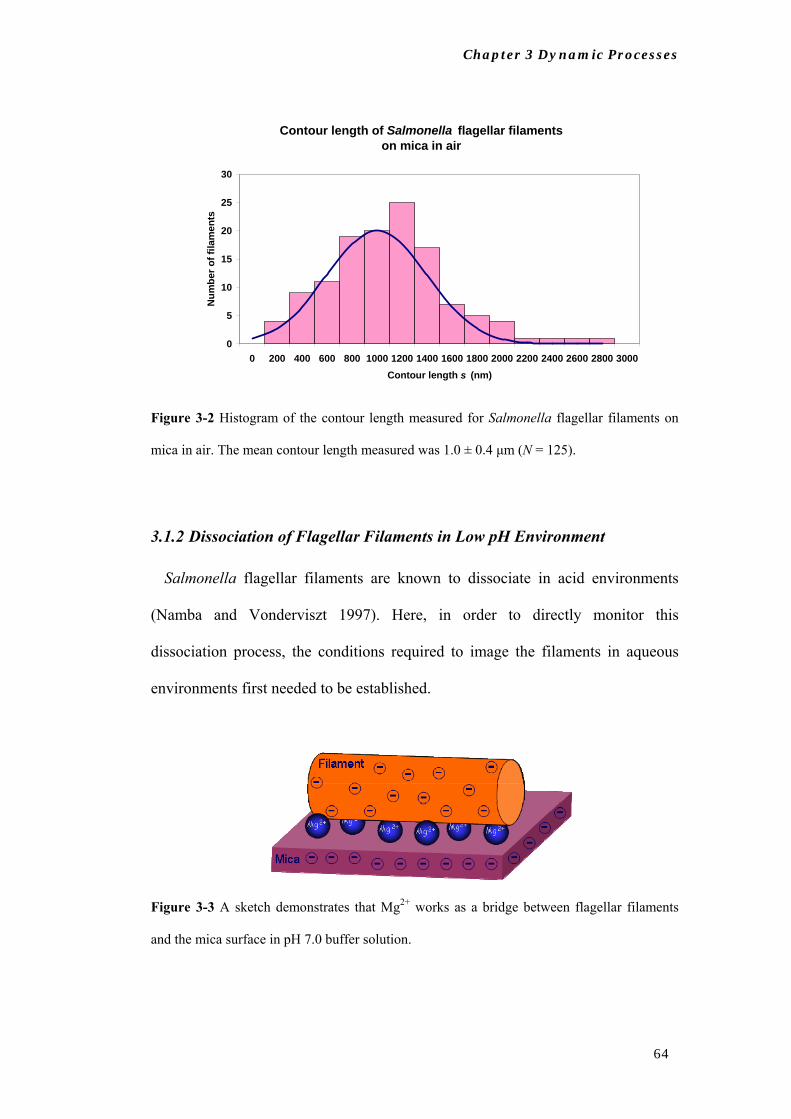
The contour length of Salmonella flagellar filaments was found to be 1.0 ± 0.4

μm (Figure 3-2). The shorter filaments are most likely the fragments resulted from

the mechanical shearing during the filaments preparation (see section 2.2.1). The

average height of the filaments was 4.5 ± 0.6 nm.

63


Contour length of Salmonella flagellar filaments on mica in air

0

5

10

15

20

25

30

0 200 400 600 800 1000 1200 1400 1600 1800 2000 2200 2400 2600 2800 3000Contour length s (nm)

Num

ber o

f fila

men

ts

Figure 3-2 Histogram of the contour length measured for Salmonella flagellar filaments on

mica in air. The mean contour length measured was 1.0 ± 0.4 μm (N = 125).

3.1.2 Dissociation of Flagellar Filaments in Low pH Environment

Salmonella flagellar filaments are known to dissociate in acid environments

(Namba and Vonderviszt 1997). Here, in order to directly monitor this

dissociation process, the conditions required to image the filaments in aqueous

environments first needed to be established.

Figure 3-3 A sketch demonstrates that Mg2+ works as a bridge between flagellar filaments

and the mica surface in pH 7.0 buffer solution.

64


Because the isoelectric point (pI) of flagellin is 5.2 and the amino acid residues

on the outer surface of Salmonella flagellar filaments are mostly charged residues

(Namba and Vonderviszt 1997), in pH > 5.2 solution, the surface of Salmonella

flagellar filaments will be negatively charged; as is the surface of the mica

substrate (Vesenka et al. 1992). Therefore, without the inclusion of additional ions,

the imaging of the Salmonella flagellar filaments on mica substrates is

problematic due to poor immobilization. Two methods were explored to resolve

this problem. First, magnesium ions (Mg2+) were added into solution to

immobilize the Salmonella flagellar filaments onto the mica surface (Figure 3-3)

(Vesenka et al. 1992, see section 3.1.1 and 3.1.3); second, AFM images were

obtained at a pH at least lower than 5.2 (see section 3.1.2).

3.1.2.1 Salmonella Flagellar Filaments in Neutral Condition

Salmonella flagellar filaments were first imaged in pH 7.0 solution. A height

image taken in pH 7.0 buffer solution (10 mM PBS & 10 mM MgCl2) using

tapping mode AFM is displayed on Figure 3-4. To prepare samples for imaging,

stock solution of Salmonella flagellar filaments (for preparation of stock solution

see section 2.2.1) was diluted 100 fold using pH 7.0 buffer solution (10 mM PBS

& 10 mM MgCl2). A 10 μL droplet of diluted sample solution was spread on a

freshly cleaved mica surface, and left for 1hour on mica, before covering with pH

7.0 buffer solution (10 mM PBS & 10 mM MgCl2) for AFM imaging. There are

two long filaments and two short filaments visible in Figure 3-4. Some very short

flagellar filament fragments can also been seen in Figure 3-4, which were probably

produced during the mechanical shearing process when the flagellar filaments

were removed from the living cells (see section 2.2.1).

65


Figure 3-4 A height image of Salmonella flagellar filaments taken in pH 7.0 buffer solution

(10 mM PBS & 10 mM MgCl2) using tapping mode AFM. The Z-range is 9.3 nm.

3.1.2.2 Salmonella Flagellar Filaments in Weak Acidic Condition

As stated above, in low pH solution (pH<5.2), Salmonella flagellar filaments

would be positively charged, therefore, they could be immobilized directly onto

the mica surface via electrostatic attraction. A height image taken in pH 4.4

solution using tapping mode AFM is displayed in Figure 3-5. Stock solution of

Salmonella flagellar filaments was diluted 100 fold by HCl to achieve a final pH

of 4.4 for AFM imaging. A 10 μL droplet of sample solution was spread on a

freshly cleaved mica surface and left for 1.5 h before covering with HCl (pH 4.4)

solution for AFM imaging.

66


Figure 3-5 A height image of Salmonella flagellar filaments taken in HCl solution (pH 4.4)

using tapping mode AFM. The Z-range is 14.2 nm.

3.1.2.3 Salmonella Flagellar Filaments in Alkaline Condition

Salmonella flagellar filaments were also imaged in alkaline solution, with the

presence of Mg2+ ions. A height image taken in pH 10.0 solution (0.1mM NaOH

& 10 mM MgCl2) using tapping mode AFM is displayed on Figure 3-6. The stock

solution of Salmonella flagellar filaments was diluted 100 fold with solution

(0.1mM NaOH & 10 mM MgCl2) to a final pH of 10.0 for AFM imaging. A 10

μL droplet of sample solution was spread on a freshly cleaved mica surface and

allowed to stand for 1h before covering with solution (0.1mM NaOH & 10 mM

MgCl2, pH 10.0) for AFM imaging.

67


Figure 3-6 A height image of Salmonella flagellar filaments taken in pH 10.0 solution

(0.1mM NaOH & 10 mM MgCl2) using tapping mode of AFM. The Z-range is 22.6 nm.

The results of AFM experiments of Salmonella flagellar filaments in acidic,

alkaline and neutral environments are presented in Table 3-1 for comparison. The

dimensions were measured using SPIP software (see section 2.1.3).

The cross section of Salmonella flagellar filaments is known to be circular

(Mimori et al. 1995; Morgan et al. 1995). However, measured from AFM images,

the diameters were found to be bigger than the height measurements (Table 3-1).

This may because of three reasons: First, it may be due to tip broadening

phenomena. Tip broadening arises when the radius of curvature of the tip is

comparable with, or greater than, the size of the feature being imaged (West and

Starostina n.d.). The diagram in Figure 3-7 illustrates this problem. As the tip scans

over the filament, the sides of the tip make contact before the apex, and the

microscope begins to respond to the feature. Second, the pressure caused by the

AFM tip may also result in compression of the Salmonella flagellar filaments

68


(Morris et al. 1999). Third, the attraction between the Salmonella flagellar

filaments and the mica surface may also result in some compression and a

decrease the height of the filaments (Israelachvili 1992).

Table 3-1 The dimensions of Salmonella flagellar filaments observed in AFM images

obtained in liquid.

pH of the solutions pH 4.4 pH 7.0 pH 10.0

Diameter D (nm) 33.7 ± 0.8 26.8 ± 0.8 34.2 ± 0.9

Height H (nm) 7.2 ± 0.6 9.1 ± 0.5 7.1 ± 0.6

Length L (μm) 1.0 - 3.0

N 5 8 10

N is the number of Salmonella flagellar filaments measured; D is the average diameter of

Salmonella flagellar filaments; H is the average height of Salmonella flagellar filaments; L is

the length range of the most Salmonella flagellar filaments observed. All the images were

taken in liquid using tapping mode AFM and analyzed using SPIP software (see section

2.1.3).

Example of an AFM tip

A filament

AFM image: apparent width

Example of an AFM tip

A filament

AFM image: apparent width

Figure 3-7 Sketch of an example of "tip broadening" effect on a filament. On the bottom a

resulting scan line is shown.

69


Although the dimensions of Salmonella flagellar filaments in AFM images may

be affected by the difference of the AFM tips and/or the imaging conditions

employed (e.g. set point), the observed dimensions may still provide useful

information on the environmental effect on the filaments. For example, the

average diameter of Salmonella flagellar filaments measured in pH 4.4 solution

was ~33% wider than in pH 7.0 solution; while the average height measured in pH

7.0 solution was ~24% less in pH 4.4 solution. This may because Salmonella

flagellar filaments were “softer” and more compressible by AFM tip under low

pH environment.

The height and the diameter of the filaments in alkaline solution are close to the

dimensions of the filaments in weak acidic solution, which indicates that the

conformations of Salmonella flagellar filaments in acidic and alkaline

environments may be similar (Kamiya and Asakura 1976; also see section 1.2.2.3).

3.1.2.4 Dissociation of Salmonella Flagellar Filaments in Acidic Condition

Salmonella flagellar filaments are not stable in low pH environments (pH<4.4),

where they are likely to be dissociated into single flagellin proteins (Namba and

Vonderviszt 1997).

70


Figure 3-8 A height image of Salmonella flagellar filaments taken in pH 4.0 solution using

tapping mode of AFM. The Z-range is 8.8 nm.

A height image of Salmonella flagellar filaments taken in pH 4.0 solution using

tapping mode AFM is displayed in Figure 3-8. Sample solution was allowed to

stand for 1 h on mica before imaging. The average height of the particles observed

in this image is 2.4 ± 0.3 nm. The particles are most likely single flagellin or

subunits of several flagellins (Namba and Vonderviszt 1997). From the sample

preparation of these images it was clear that Salmonella flagellar filaments

dissociated in pH 4.0 solution within 1 h. Therefore to directly observe the

process of dissociation, the experiment of changing the pH of solution while

imaging was performed.

71


3.1.2.5 Direct Observation of the Dissociation of Salmonella Flagellar

Filaments in Acidic Condition

The dissociation of Salmonella flagellar filaments in acidic solution is shown in

Figure 3-9. Three filaments were initially imaged in pH 7.0 PBS solution. Image (a)

was taken right after the injection of 1mM HCl into the fluid cell (see section

2.2.5), no visible dissociation was observed. Image (b) was taken 20 minutes after

the injection. Most parts of the three filaments had undergone a dissociation

process, though several fragments of filaments could still be seen (e.g. a fragment

in the centre of the cross) in image (b). Image (c) was taken 40 minutes after the

injection. There were almost no fragments remaining in image (c). Image (d) was

taken 1 hour after the injection. The filaments were completely dissociated into

particles and diffusing away from the original site.

Figure 3-9 Height images of Salmonella flagellar filaments in liquid using tapping mode

AFM. The sample was in pH 7.0 buffer solution (10 mM PBS & 10 mM MgCl2) at first, then

1mM HCl was injected into the sample solution. (a) was taken right after injection; then (b)

was taken 20 min after injection; (c) was taken 40 min after injection; (d) was taken 1 h after

injection. The Z-range is 9.9 nm.

72


This was the first time that the dissociation process of Salmonella flagellar

filaments in low pH solution has been visualised by AFM. This study provided

highly valuable information for the development of applications for Salmonella

flagellar filaments. Most of the intersubunit interactions found within the outer

tube of flagellar filaments are polar–polar or charge–polar (Yonekura et al. 2002;

2003; also see section 1.2.2). When basic residues are protonated, the interactions

between flagellin break down. All parts of a filament exposed to the low pH

solution were found to break down instantly. The centre piece fragment of the

cross in image Figure 3-9 (b) was probably a fragment from the lower filament of

the cross on image (a), which survived in the first 20 minutes because of the

protection of the upper filament of the cross from the low pH solution. This could

be used advantageously in the controlled digestion of flagellar filaments when

flagellar filaments are used as scaffolds to obtain nanowires (Kumara et al. 2006;

2007; Woods et al. 2007, also see section 1.2.3).

3.1.3 Flagellar Filaments on Gold Surface

Salmonella flagellar filaments on gold substrate also studied. It is part of the

study to explore the imaging capability of AFM in different environment, as well

as the foundation for studies on physical properties in later chapters (e.g. chapter 4

and 6).

3.1.3.1 Salmonella Flagellar Filaments imaged in Air on Gold Surfaces

Gold substrates were prepared by coating gold onto freshly cleaved mica

surface using evaporation gold coater (see section 2.2.5). Stock solutions of

Salmonella flagellar filaments were diluted 100 times using pH 7.0 buffer solution

73


(10 mM PBS) and then imaged using tapping mode AFM in air on gold (Figure

3-10; detailed sample preparation see section 2.2). The average height of the

Salmonella flagellar filaments observed on the gold substrates was 4.4 ± 0.6 nm

(N = 20).

Figure 3-10 Tapping mode AFM height images of Salmonella flagellar filaments in air on

gold. Stock sample solutions were 100 times diluted. The Z-scale is 351.5 nm.

3.1.3.2 The Salmonella Flagellar Filaments in Propanol on Gold Surface

It was found difficult to immobilize Salmonella flagellar filaments onto gold

substrate while scanning in aqueous buffer solution. However, in propanol or

water mixed with propanol (>80% propanol), Salmonella flagellar filaments were

found to bind to the substrate firmly enough to allow imaging (Figure 3-11). This

may be due to the dehydration and/or the insolubility of Salmonella flagellar

filaments in propanol solutions. The dehydration may help to expose the filaments

74


surface to the probing tip (Hansma et al. 1992; 1993; Lyubchenko et al. 1993).

The influence of imaging condition on the observed filament dimensions was

investigated by imaging in a series of propanol-water mixtures (Table 3-2) (Figure

3-12).

Figure 3-11 Tapping mode AFM height images of Salmonella flagellar filaments in 80%

propanol on gold. Stock sample solutions were 5 times diluted.

Table 3-2 The average height of Salmonella flagellar filaments on gold surface in a series of

propanol-water mixtures.

Buffer 100% propanol 90% propanol + 10% water 80% propanol + 20% water

Height (nm) 5.4 ± 0.5 12.2 ± 0.9 17.0 ± 1.1

75


y = -0.58x + 63.733R 2̂ = 0.9902

0

2

4

6

8

10

12

14

16

18

20

75 80 85 90 95 100Percentage of Propanol in Buffer (%)

Aver

age

Hei

ght o

f Sal

mon

ella

Fla

gella

r Fila

men

ts (n

m)

Figure 3-12 A plot of average height of Salmonella flagellar filaments vs. percentage of

propanol in propanol-water buffer.

In 100% propanol, the average height of Salmonella flagellar filaments was

close to that observed in air; the average height increased proportionally while the

percentage of propanol in buffer decreased. In below a concentration of 70%

propanol, Salmonella flagellar filaments could not be immobilized onto gold.

3.2 Fibrillization Processes of Lysozyme

Unlike the dissociation of Salmonella flagellar filaments in low pH

environments which occurred within an hour, the fibrillization of lysozyme takes

up to two weeks in laboratory (Krebs, et al. 2000, also see section 2.2.2).

Therefore, real-time monitoring of this fibrillization process by AFM imaging is

not feasible. In order to observe it, the assembly process has to be interrupted, so

that samples can be prepared for AFM analysis.

76


3.2.1 Preparation of Lysozyme Samples

Lysozyme protein dissolved in glycine buffer was incubated at 57 ± 2 °C

(details see section 2.2.2). After a certain incubation time, the sample was

removed from the oven to room temperature and a 10 µL droplet of sample

solution spread onto a fleshly cleaved mica surface. After 2 minutes, the mica

surface was rinsed with distilled water, and then dried under a gentle flow of

nitrogen gas. The sample then was imaged with AFM using tapping mode in air

(Figure 3-16 to Figure 3-23). This AFM sample preparation process, especially the

drying procedure stopped the continuous fibrillization of lysozyme.

Glycine buffer was imaged under the same conditions before and after

incubation as the control experiment (Figure 3-13). A few particles (height range

from ~2 nm to ~10 nm) were observed on the images, which we attribute to

undissolved glycine powder produced when the buffer was prepared.

The initial lysozyme sample was also imaged prior to incubation (Figure 3-14).

Lysozyme protein is known to have hydrodynamic diameter of 4.1nm (Merrill, et

al., 1993). Particles of lysozyme proteins were observed on the AFM images. The

average height of lysozyme particles measured from AFM images was 1.6 ± 0.5

nm. A histogram of the height of lysozyme particles was displayed in Figure 3-15.

The particles observed are most likely single lysozyme proteins or clusters of

several lysozyme proteins. The average height obtained however was smaller than

the previously known diameter of lysozyme protein. The reduction of the diameter

is most likely due to the drying process during the sample preparation and/or the

pressure caused by the AFM probe while scanning (Rossell 2003).

77


Figure 3-13 An AFM height image of 10 mM glycine buffer obtained using tapping mode

AFM before (a) and after (b) incubation at 57 ± 2 °C for 2 weeks. The Z-range is 8.1 nm.

78


Figure 3-14 An AFM height image in tapping mode of 10mg/mL lysozyme in 10mM glycine

buffer at pH 2.0. The Z-range is 9.8 nm.

Figure 3-15 Histogram of the height of lysozyme particles before incubation measured from

AFM images taken on mica in air. The average height of lysozyme particles was 1.6 ± 0.5 nm

(N = 136).

79


3.2.2 The Early Stages of Lysozyme Fibrillization

Samples from different batches were found to have slightly different rates of

fibrillization. Highly flexible protofilaments of elongated lysozyme proteins were

however always observed after 2 to 3 days of incubation (Figure 3-16).

Figure 3-16 An AFM height image of lysozyme after 3 days of incubation. A 3D image

(generated by SPIP software) of one protofilament, which is indicated by the black arrow, is

displayed on the left. The Z-range is 10.4 nm.

The protofilament appeared to be a chain of single particles (Figure 3-16, Jansen

et al. 2005; Goldsbury et al. 2005). The lengths of the protofilaments were from

~80 nm to ~700 nm. The average height of the higher points of the protofilaments

was 4.4 ± 0.6 nm; while the average height of the lower points of the

protofilaments was 2.9 ± 0.2 nm. Compared to the height of the single lysozyme

proteins (1.6 ± 0.5 nm), the elongated particles were (4.4 / 1.6 =) 2.8 times in

80


height. This suggested that lysozyme proteins had undergone a dramatic structural

change in order to form protofilaments (Dobson et al., 1998).

After 2 to 3 days of incubation, along with the protofilaments, a few fibrils with

clear periodicities began to be observed. One such fibril is shown in Figure 3-17.

This fibril has a pitch of 85 ± 4 nm, an average height 5.3 ± 0.9 nm with the

average height of the higher points 7.0 ± 0.3 nm and average height of the lower

points 3.5 ± 0.1 nm (Jansen et al. 2005).

Figure 3-17 AFM image of one lysozyme fibril with clear periodicity after 2 days of

incubation; (a) is the height image, (b) is the profile along the axis of the fibril on (a), and (c)

is a 3D image of the fibril on (a) generated by SPIP software (see section 2.1.3). The pitch of

this fibril is 85 ± 4 nm. The average height of this fibril is 5.3 ± 0.9 nm with the average

height of the higher points 7.0 ± 0.3 nm and average height of the lower points 3.5 ± 0.1 nm.

The Z-range is 20.5 nm.

81


3.2.3 The Middle Stages of Fibrillization

Fibrils with distinct branches splaying apart (Figure 3-18, indicated by green

arrows) were observed after 4 days of incubation. The highly flexible

protofilaments (Figure 3-18, indicted by blue arrows) have an average height of 2.3

± 0.2 nm.

Figure 3-18 AFM height image of lysozyme fibrils after 4 days of incubation. The green

arrows indicate fibrils with distinct branches splaying apart. The pink arrows indicate highly

flexible protofilaments connected to rigid mature fibrils. The Z-range is 15.9 nm.

Lysozyme fibrils from three different batches on the middle stages of incubation

(2 to 10 days) were imaged and categorised according to their heights into 6 types

(Table 3-3).

As described in section 1.3.1.3, Khurana and co-workers (2003) proposed a

general hierarchical assembly model of amyloid fibrils. For example, the

assembly model of insulin into amyloid fibrils is as shown in Figure 3-19. Two

identical subunits intertwine with each other to form fibrils of a higher assembly

82


level. The subunit can be a protofilament or a fibril consisting of 2 or 4

protofilaments, and the average height of a fibril is 1.5D (D is the diameter of the

cross section of a subunit), with the height of the higher points 2D and the height

of the low points D.

Table 3-3 The average heights of 6 types of lysozyme fibrils observed. Types II to VI fibrils

have clear periodicity. Type I fibrils did not have clear periodicity.

Type I Type II Type III Type IV Type V Type VI

Average height of

higher points (nm) 4.5 ± 0.3 5.7 ± 0.1 7.0 ± 0.3 7.2 ± 0.2 10.2 ± 0.2

Average height of

lower points (nm)

2.3 ± 0.2

2.5 ± 0.2 3.8 ± 0.1 3.5 ± 0.2 5.4 ± 0.2 6.0 ± 0.1

N 50 30 30 20 9 6

If the assembly of lysozyme fibrils also followed the same model as in Figure

3-19, from the height of lysozyme protofilaments (2.3 ± 0.2 nm), the Type I fibrils,

the heights of the fibrils would be predicted as shown in Table 3-4.

Compared Table 3-4 with Table 3-3, Type II lysozyme fibrils fit well into “1+1”

model; Type IV fibrils fit well into “2+2” model; and Type VI fibrils fit well into

“4+4” model. However, other types of fibrils do not fit into Khurana’s model.

As indicated by pink arrows in Figure 3-18, highly flexible protofilaments were

observed connected to fibrils of different types. This may therefore suggest a new

assembly model i.e. an “n+1” model (where n is the number of protofilaments in

one subunit) (Table 3-5). In other words, a protofilament might intertwine with a

fibril already consisting of more than one protofilament (Figure 3-20). The average

83


height of an “n+1” fibril is (Dn + D1)/2 (Dn is the diameter of the cross section of

the subunit consisting of more than one protofilaments; D1 is the diameter of the

cross section of one protofilament), with the height of the higher points (Dn + D1)

and the height of the lower points Dn.

Figure 3-19 A model for the hierarchical assembly of insulin into amyloid fibrils.

Protofilament pairs wind together to form “1+1” fibrils, and two “1+1” fibrils wind to form a

“2+2” fibril. “4+4” fibrils are the result of winding of two “2+2” fibrils (figure adapted from

Khurana 2003).

Table 3-4 The predicated heights using Khurana’s model (2003).

Protofilaments 1+1 Fibrils 2+2 Fibrils 4+4 Fibrils

Height of higher points (nm) 4.6 6.9 10.4

Height of lower points (nm) 2.3

2.3 3.4 5.2

84


Figure 3-20 “n+1” model for lysozyme fibrils assembly. Protofilaments intertwine with each

other to form “1+1” fibrils. Two “1+1” fibrils intertwine into a “2+2” fibril. A protofilament

can intertwine with a “1+1” fibril to form a “2+1” fibril or with a “2+2” fibril to form a “4+1”

fibril.

Table 3-5 The predicated heights using the “n+1” model.

Protofilaments 2+1 Fibrils 4+1 Fibrils

Height of higher points (nm) 5.8 7.5

Height of lower points (nm) 2.3

3.4 5.2

85


Compared with Table 3-5 with Table 3-3, Type III lysozyme fibrils fit well into

“2+1” model, and Type V fibrils fit well into “4+1” model. The data is summed

up in Table 3-6 for comparison.

Table 3-6 The summary of the experimental data of the heights of lysozyme fibrils and the

heights predicted by Khurana’s model and “n+1” model.

Fibrils model 1+1 2+1 2+2 4+1 4+4

Average height of

higher points (nm) 4.5 ± 0.3 5.7 ± 0.1 7.0 ± 0.3 7.2 ± 0.2 10.2 ± 0.2

Experimental

data Average height of

lower points (nm) 2.5 ± 0.2 3.8 ± 0.1 3.5 ± 0.2 5.4 ± 0.2 6.0 ± 0.1

Height of higher

points (nm) 4.6 5.8 6.9 7.5 10.4

Predicted by

model Height of lower

points (nm) 2.3 3.4 3.4 5.2 5.2

Note that for the heights of the higher points, the experimental data are 4% less

to 2% more than predicated by the model. However, for the heights of the lower

points, the experimental data are 3% to 15% more than predicated by the model;

especially for the “4+4” fibrils, the experimental data is ((6.0-5.2) / 5.2 =) 15%

more than predicated by the model. This might be because the fibrils were raised

from the mica surface at the lower points due to the stiffness of the fibrils and

intertwining, which would increase the height of the lower points measured from

the profile of AFM images. Since the stiffness increased with the increasing of the

assembly level (a detailed discussion of the elasticity of the lysozyme fibrils will

86


be presented in section 4.3), the increasing of the height of the lower points of

“4+4” fibrils was more observable than other fibrils.

Using both Khurana’s model and “n+1” model, the fibrils observed on AFM

images can therefore be explained. An example is given in Figure 3-21: a “1+1”

fibril intertwines with a protofilaments to form a “2+1” fibril.

Figure 3-21 An AFM height image of a lysozyme fibril after 4 days of incubation. The fibril

indicated by green arrow has height of 2.4 ± 0.1 nm, which could be a protofilament; the fibril

indicated by pink bracket has average height of higher points 4.6 ± 0.1 nm and lower points

2.8 ± 0.1 nm, which could be a “1+1” fibril; the fibril indicated by the blue bracket has an

average height of higher points 5.5 ± 0.5 nm and lower points 3.5 ± 0.1 nm, which could be a

“2+1” fibril. The Z-range is 9.1 nm.

Some fibrils were observed to be connected to more than one fibril (Figure 3-18),

suggesting that the formation of mature fibrils from the intertwining of subunits

87


might happen starting from the two ends or even in the middle of the subunits;

also that fibrils of different assembly levels might be forming at the same time.

3.2.4 The Late Stages of Lysozyme Fibrillization

After 11 to 14 days of incubation (Figure 3-22), the sample solution started to

have a gel-like appearance. Most lysozyme fibrils appeared to have clear

periodicity with a periodicity to diameter ratio of ~20. Interestingly, some fibrils

appeared to have sinusoidal shape (Figure 3-22, indicated by pink arrows), which

might be due to some degree of unwinding of the subunits created during the

adsorption process of the fibrils to the substrate.

Figure 3-22 An AFM height image of lysozyme fibrils after 11 days of incubation. The pink

arrows indicate some fibrils with sinusoidal shape. The Z-range is 26.6 nm.

88


Circular fibrils, the diameter of which was typically 250~350 nm, were also

observed after 14 days of incubation (Figure 3-23).

Figure 3-23 AFM height images of lysozyme fibrils after 14 days of incubation. The green

arrows indicate several fibrils with circular structures. The blue arrows indicate two fibrils

with half circular structures. The image on the right has better resolution, with one circular

fibril on the middle. The Z-range of the left image is 24.3 nm.

Previous studies on solvational and hyperbaric tuning of amyloidogenesis with

insulin fibrils suggested that circular structures of amyloid fibrils are probably a

lower void volume alternative to straight fibrils (Jansen et al. 2004; Grudzielanek

et al. 2005; also see section 1.3.1.3). The fact that the circular structure of

lysozyme fibrils were only observed at the late stages of fibrillization when fibrils

became “crowded”, agreed with this theory. However, no high hydrostatic

pressure and addition of cosolvents or cosolutes were required in this case, which

89


suggests that simpler conditions could be applied to manipulate the conformation

of amyloid fibrils.

3.3 Alternative Assembly of Tubular and Spherical

Nanostructures from FF Peptides

The self-assembly of FF peptide monomers into nanotubes happens very rapidly

(Reches and Gazit 2003). In order to observe the formation of FF nanotubes, the

sample for AFM operation needs therefore to be prepared immediately after the

FF nanotubes are formed, so that further self-assembly is interrupted.

FF nanotubes prepared by Reches and Gazit’s method (2003), where FF peptide

was dissolved in HFIP at high concentrations (100mg/mL) and then diluted into

the aqueous solution at a final μM concentration range (for detailed preparation

see section 2.2.4), were typically several micrometers in length and 50 to 300 nm

in diameter (Figure 3-24). However, short and thin fibrillar structures of 2 to 4 nm

in height were also sometimes observed along with the long and thick nanotubes

(Figure 3-24). Associating with the tentative model proposed by Görbitz (2006)

(see section 1.3.3.2), the long and thick nanotubes may have their proposed

multilayer tubular wall, while the short and thin fibrils might well be single-wall

nanotubes.

90


Figure 3-24 AFM image of typical long and thick FF nanotubes along with short and thin

fibrilar structures. The long and thick FF nanotubes lying from the top left to the bottom right

on the middle of this image is whitened because the colour scale has been adjusted in order to

enhance the appearance of the short and thin fibrilar structures. The Z-range is 107.2 nm.

Song and co-workers reported (2004) another nanotube preparation method,

where FF peptide was dissolved in water to 2mg/mL at 65 °C, and the sample

equilibrated for 30 min and then gradually cooled to room temperature (Figure

3-25 a). They noted that when 0.1 mL of the nanotube mixture was diluted by

adding 0.1 mL of water, vesicles were present in addition to the nanotubes (Figure

3-25 b; also see section 1.3.3.1). Song suggested that the concentration of the

peptide is a key factor in the formation of the nanotubes. However, by noticing the

presence of vesicles in the SEM image of FF nanotubes before dilution in Song’s

paper (Figure 3-25 a, indicated by pick arrows), I suspected that the temperature

might play an important role in the alternative formation of tubular and spherical

structures. Bearing this in mind, I used modified Reches and Gazit’s (2003)

91


method to investigate the effect of temperature on the formation of FF

nanostructures.

Figure 3-25 SEM images of (a) peptide nanotubes and (b) a mixture of nanotubes and

vesicles (figure and caption adapted from Song et al. 2003, Fig 1)

FF peptide HFIP stock solution (100mg/mL) and distilled water were pre-

warmed in a 40˚C water bath. The AFM sample (2mg/mL) was then prepared

using this stock solutions and distilled water (detailed preparation see section

2.2.4). An AFM topography image of this sample is displayed in Figure 3-26.

Spherical structures of 2 to 4 nm in height were observed. Thin fibrilar structures

of ~1 nm in height, 200 to 300 nm in length were also observed.

In a similar manner, the FF peptide HFIP stock solution (100mg/mL) and

distilled water were pre-warmed in 65˚C water bath. The AFM sample (2mg/mL)

then prepared using these stock solution and distilled water. An AFM topography

92


image of this sample is displayed in Figure 3-27. Spherical structures of 2 to 4 nm

in height were observed. However, no tubular structures were observed.

As stated before, results from original Reches and Gazit’s (2003) method had

only nanotubes but no spherical strutures observed. Comparing the results from

modified Reches and Gazit’s method, it seemed that the temperature is likely to be

a key factor in the alternative assembly of tubular and spherical nanostructures

during FF self-assembly. The tubular structures might be kinetically favoured

(Reches and Gazit 2004).

Reches and Gazit have also reported (2004) the formation of spherical

nanostructures of diphenylglycine peptide, a highly similar analogue of

diphenylalanine peptide. Comparing this to the formation of spherical

nanostructures of FF peptides, the diphenylglycine peptide might have lower

energy barrier to form spherical nanostructures. By controlling the temperature,

the formation of tubular structures from diphenylglycine peptide or other

analogues of FF peptide might therefore be possible.

93


Figure 3-26 An AFM image of FF nanostructures self-assembled at 40˚C. A few thin fibrilar

structures of ~1 nm in height, 200 to 300 nm in length were observed along with spherical

structures of 2 to 4 nm in height. The Z-range is 21.7 nm.

Figure 3-27 An AFM image of FF nanostructures self-assembled at 65˚C. Spherical

structures of 2 to 4 nm in height were observed. The vesicles lie in lines, which is most likely

due to the drying process during sample preparation. The Z-range is 6.2 nm.

94


3.4 Conclusion

In this chapter, the imaging capability of AFM has been explored and a range of

imaging studies monitoring the dynamic processes of protein nanotubes have been

presented. A better understanding of the dynamic processes of protein nanotubes,

provides the information on manipulating these protein nanotubular materials,

which is desired in order to utilize them in applications.

The dissociation process of Salmonella flagellar filaments in low pH solution

was found to happen within an hour; therefore, real-time monitoring was possible.

All parts of a filament exposed to the low pH solution were found to instantly

break down to single flagellin proteins at the same time.

If the dynamic process of protein nanotubes occurs on timescales that are too

long or too short for real-time AFM monitoring, the process has to be interrupted

so that the sample can be prepared for AFM operation. For example, the

fibrillization process of lysozyme fibrils takes up to two weeks, while the

formation of nanostructures from FF peptides takes only a few seconds to a few

minutes.

By observing the fibrillization process of lysozyme fibrils, the “n+1” model has

been proposed: a protofilament may intertwine with a fibril consisting of more

than one protofilament to form higher assembly level fibrils. This model

complements the hierarchical assembly model proposed by Khurana (2003).

The effect of temperature on the alternative formation of tubular and spherical

nanostructures of FF peptides was also investigated, which may suggest a general

way of controlling the formation of nanostructures from FF peptides and its

similar analogues.

95

Documents

Chapter 2 Instrumental and Experimental Methods - … · Chapter 2 Instrumental and Experimental Methods . ... Conversion of force curves . ... (Albrecht . et al. 1990; Butt