Embed Size (px)
Citation preview
20
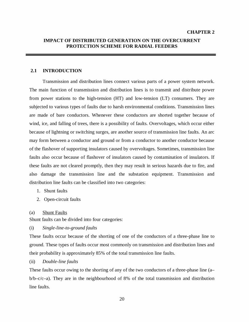
CHAPTER 2
IMPACT OF DISTRIBUTED GENERATION ON THE OVERCURRENT PROTECTION SCHEME FOR RADIAL FEEDERS
2.1 INTRODUCTION
Transmission and distribution lines connect various parts of a power system network.
The main function of transmission and distribution lines is to transmit and distribute power
from power stations to the high-tension (HT) and low-tension (LT) consumers. They are
subjected to various types of faults due to harsh environmental conditions. Transmission lines
are made of bare conductors. Whenever these conductors are shorted together because of
wind, ice, and falling of trees, there is a possibility of faults. Overvoltages, which occur either
because of lightning or switching surges, are another source of transmission line faults. An arc
may form between a conductor and ground or from a conductor to another conductor because
of the flashover of supporting insulators caused by overvoltages. Sometimes, transmission line
faults also occur because of flashover of insulators caused by contamination of insulators. If
these faults are not cleared promptly, then they may result in serious hazards due to fire, and
also damage the transmission line and the substation equipment. Transmission and
distribution line faults can be classified into two categories:
1. Shunt faults
2. Open-circuit faults
(a) Shunt Faults Shunt faults can be divided into four categories:
(i) Single-line-to-ground faults
These faults occur because of the shorting of one of the conductors of a three-phase line to
ground. These types of faults occur most commonly on transmission and distribution lines and
their probability is approximately 85% of the total transmission line faults.
(ii) Double-line faults
These faults occur owing to the shorting of any of the two conductors of a three-phase line (a–
b/b–c/c–a). They are in the neighbourhood of 8% of the total transmission and distribution
line faults.
21
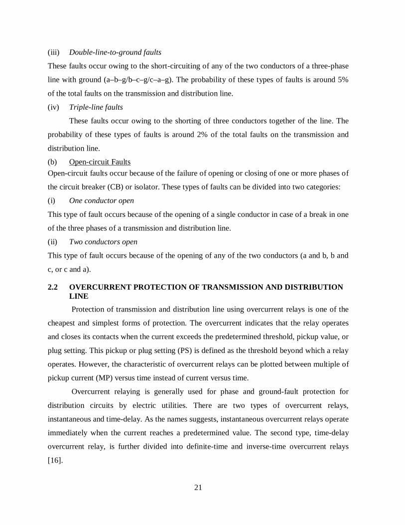
(iii) Double-line-to-ground faults
These faults occur owing to the short-circuiting of any of the two conductors of a three-phase
line with ground (a–b–g/b–c–g/c–a–g). The probability of these types of faults is around 5%
of the total faults on the transmission and distribution line.
(iv) Triple-line faults
These faults occur owing to the shorting of three conductors together of the line. The
probability of these types of faults is around 2% of the total faults on the transmission and
distribution line.
(b) Open-circuit Faults Open-circuit faults occur because of the failure of opening or closing of one or more phases of
the circuit breaker (CB) or isolator. These types of faults can be divided into two categories:
(i) One conductor open
This type of fault occurs because of the opening of a single conductor in case of a break in one
of the three phases of a transmission and distribution line.
(ii) Two conductors open
This type of fault occurs because of the opening of any of the two conductors (a and b, b and
c, or c and a).
2.2 OVERCURRENT PROTECTION OF TRANSMISSION AND DISTRIBUTION LINE Protection of transmission and distribution line using overcurrent relays is one of the
cheapest and simplest forms of protection. The overcurrent indicates that the relay operates
and closes its contacts when the current exceeds the predetermined threshold, pickup value, or
plug setting. This pickup or plug setting (PS) is defined as the threshold beyond which a relay
operates. However, the characteristic of overcurrent relays can be plotted between multiple of
pickup current (MP) versus time instead of current versus time.
Overcurrent relaying is generally used for phase and ground-fault protection for
distribution circuits by electric utilities. There are two types of overcurrent relays,
instantaneous and time-delay. As the names suggests, instantaneous overcurrent relays operate
immediately when the current reaches a predetermined value. The second type, time-delay
overcurrent relay, is further divided into definite-time and inverse-time overcurrent relays
[16].
22
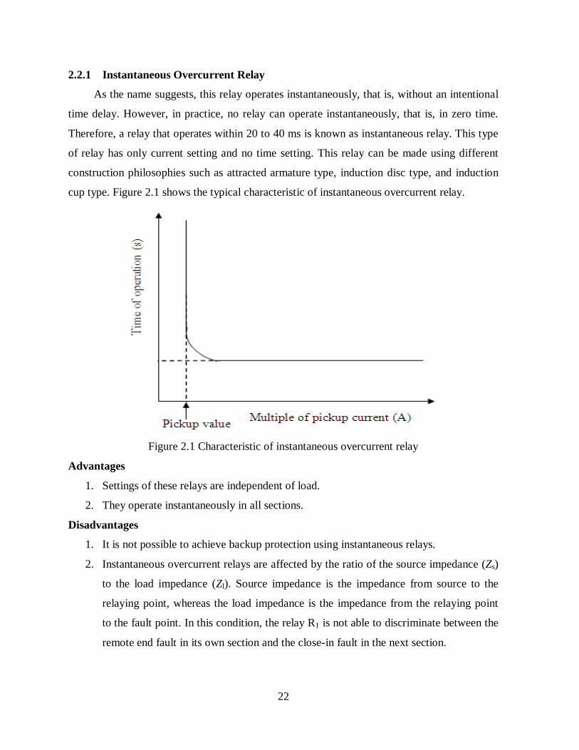
2.2.1 Instantaneous Overcurrent Relay
As the name suggests, this relay operates instantaneously, that is, without an intentional
time delay. However, in practice, no relay can operate instantaneously, that is, in zero time.
Therefore, a relay that operates within 20 to 40 ms is known as instantaneous relay. This type
of relay has only current setting and no time setting. This relay can be made using different
construction philosophies such as attracted armature type, induction disc type, and induction
cup type. Figure 2.1 shows the typical characteristic of instantaneous overcurrent relay.
Figure 2.1 Characteristic of instantaneous overcurrent relay
Advantages
1. Settings of these relays are independent of load.
2. They operate instantaneously in all sections.
Disadvantages
1. It is not possible to achieve backup protection using instantaneous relays.
2. Instantaneous overcurrent relays are affected by the ratio of the source impedance (Zs)
to the load impedance (Zl). Source impedance is the impedance from source to the
relaying point, whereas the load impedance is the impedance from the relaying point
to the fault point. In this condition, the relay R1 is not able to discriminate between the
remote end fault in its own section and the close-in fault in the next section.
23
3. Instantaneous overcurrent relays suffer from the problem of transient overreach.
Transient overreach is defined as the tendency of a relay to operate instantaneously for
faults beyond its section. This is related to the time constant of the decaying DC
component of fault current. Fault current is always asymmetric in nature. Whenever a
fault occurs, this asymmetry depends on the instant of fault occurrence. If a fault
occurs at a maximum voltage (V = Vm), there is no asymmetry, whereas for a fault at
zero voltage (V = 0), the asymmetry is maximum. The transient overreach is more if
the decay of the DC component of fault current is slow. Time delay relays are not
affected by the transient overreach phenomena.
2.2.2 Definite Time Overcurrent Relay
Definite time overcurrent relay is a relay that operates after a definite period of time
once the current exceeds the pickup value. Hence, this relay has current setting range as well
as time setting range. The current setting range is of the order of 50–200% of In, where In is
the relay-rated current. Time setting ranges are of the order of 0.1–1 s, 1–10 s, or 6–60 s. In
electromechanical relay, the relay characteristic can be achieved by the following equation.
KTMSMP
AT pop 1)(
(2.1)
where,
Top = time of operation of a relay in seconds.
TMS is time multiplier setting, MP is the multiple of pickup current and it is also known as
plug setting multiplier (PSM) and given by the following equation.
RatioCTPSInjectedCurrentFaultPSM
(2.2)
A, p, and K are the circuit constants that decide relay characteristics. For definite time
overcurrent relay K = 0, and A and p are very small (close to zero). Figure 2.2 shows the
typical characteristic of definite minimum time overcurrent relay.
Advantages
1. It provides backup protection.
2. It is immune to the ratio of source impedance to load impedance (Zs/Zl).

24
Figure 2.2 Characteristic of definite time overcurrent relay
Disadvantages
It is to be noted from Figure 2.2 that the time of operation (Top) of relay for a
fault near the generator can be dangerously high. This is obviously undesirable
because of the fact that the magnitude of such faults is very high. If these faults
persist for a long period of time, then they produce destructive effect. The
solution to this problem is to use instantaneous high set unit along with definite
time delay unit. Another solution to this type of problem is to use inverse time
overcurrent relay, which is explained in next Section.
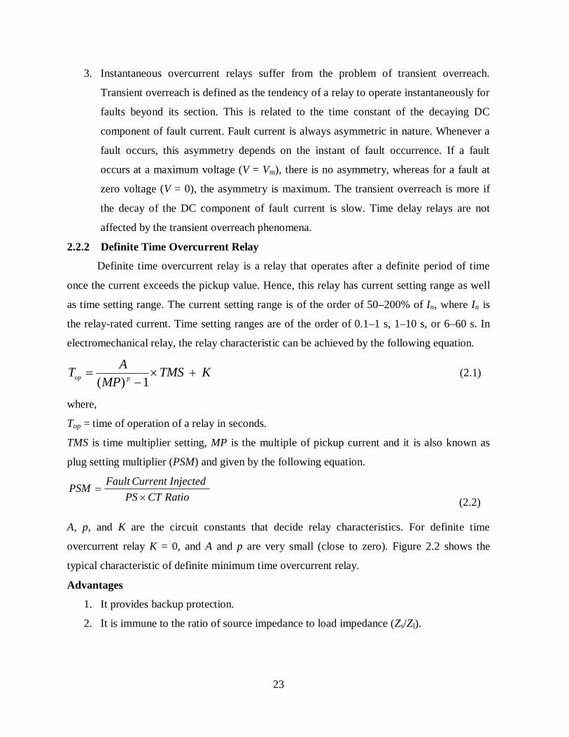
2.2.3 Inverse Time Overcurrent Relay As the name suggests, the time of operation of this relay is inversely proportional to
fault current. This is most widely used relay as it operates very quickly for a fault near the
source. This is very important as the more severe faults are cleared quickly. With the advent
of digital relays, it is possible to generate any type of inverse time overcurrent relay
characteristics. However, as the electromechanical relays are still widely used in substations,
one has to use a characteristic that can easily be matched with the available electromechanical
relay characteristic. Figure 2.3 shows normal inverse, very inverse, and extremely inverse
characteristics of the inverse time overcurrent relay.
25
Figure 2.3 Characteristic of inverse time overcurrent relay
2.2.4 Inverse Definite Minimum Time Overcurrent Relay This type of relay is widely used by the utilities in the field. Initially, the characteristic
of the relay follows inverse law, and thereafter, when the current becomes very high, it
follows definite minimum operating time pattern. This is because of the constant operating
torque due to the saturation of flux at a high value of current in the electromechanical relay.
The characteristic of IDMT relay is shown in Figure 2.3.
Advantages
1. Inverse time overcurrent relays operate faster for faults near the generator (source).
2. They provide backup protection.
3. They maintain selectivity criteria of the protection system.
4. In order to reduce the time of operation of inverse time overcurrent relays near the
generator, an instantaneous high set unit is used along with inverse time unit. The
instantaneous unit is set to operate for the faults near the generator, whereas for the
faults in the remaining section, the inverse time overcurrent relay operates.
Disadvantages
1. The time of operation of inverse time overcurrent relays is very small for high value of
fault current. Hence, it is extremely difficult to decide relay settings. The remedy for
this problem is to use an IDMT relay instead of an inverse time relay. In this case, the

26
operating time of the relay remains constant for a particular high value of fault current.
Therefore, the IDMT relay follows inverse time–current pattern for small values of
fault current and definite time characteristic for large values of fault current.
2. In case of a multi-section radial feeder where Zs is very large compared to Zl, it is not
possible to achieve any significant difference in the time of operation of inverse time
overcurrent relays having normal inverse characteristics located at the far end, because
of the insignificant magnitude of fault current. The remedy for this problem is to use
very inverse or extremely inverse characteristics, which give more stepper
characteristics than the normal inverse characteristics.
3. The characteristic of load-end relay is coordinated with the characteristic of fuse. The
characteristic of extremely inverse time overcurrent relay closely matches with the
characteristic of fuse. Hence, lower TMS can be selected for load-end relay, and
similarly, lower TMSs are selected for relays located towards source.
4. The settings of inverse time overcurrent relays are highly affected by the change in
source impedance. This condition arises because of the change in loading conditions.
In this condition, there is a possibility of reduction of magnitude of the fault current
below the full load current of the feeder. In this situation, it is not possible to set the
overcurrent relay because if it is set to operate at minimum fault current, it would not
allow the feeder to draw full load current during the increase in load; and if it is set
considering the full load current, then it would not operate in case of fault current that
is lower than the full load current. Though the magnitude of fault current is lower than
the full load current, it is harmful to the system and equipments as it produces voltage
dip and negative and zero-sequence currents during unsymmetrical faults. The remedy
for this problem is to monitor inverse time overcurrent relay using an under-voltage
relay.
2.2.5 Phase and Ground Relays
In overcurrent protection of transmission lines, the protection against phase faults that
do not involve ground is carried out by phase relays. On the other hand, the protection against
ground faults is provided by separate ground relays.
The procedure of relay coordination is usually performed starting from load end, also
known as downstream end of the network, and progressing towards the source end, also
27
known as upstream end. The following are the points required to be considered during the
coordination of phase relays.
(i) Plug Setting
1. The phase relay shall reach at least up to the end of the next substation for double-line
fault with maximum source impedance (minimum generation). Similarly, the ground
relay shall reach at least up to the end of the next substation for single-line-to-ground
fault with minimum generation. The value of PS is always greater than the maximum
full load current of the line. However, this rule is not applicable to two successive
ground relays where star–delta transformer is situated.
2. While deciding the PS of any relay with reference to another relay, the relay pickup
varies from 105% to 130% of the PS of the relay.
3. Plug settings of ground relays are lower than phase relays. This is because of the fact
that the magnitude of earth-fault current is reduced owing to the tower footing
resistance, fault resistance, ground resistance, and zero-sequence impedance of the
system. Further, ground relays are usually connected in the residual circuit of three
line CTs. Hence, while deciding the PS of ground relays, we have to consider the
excitation current of CT.
(ii) Time Multiplier Setting
1. The TMS of a relay is selected in such a way that the downstream relay (relay located
near load) achieves the lowest possible time of operate for overload or fault near the
load. As we move towards the upstream relay (relay located near source), the value of
TMS progressively increases. The TMS is chosen such that it gives the desired
selective interval from the downstream relay at maximum fault conditions (for phase
relays, the triple-line fault just beyond the next relay is considered, whereas for ground
relays, single-line-to-ground fault beyond the next relay is considered).
2. Fault current calculations are usually carried out by considering the impedances of all
associated equipments in per unit.
3. While deciding the TMS of an upstream relay with reference to the downstream relay,
proper minimum coordination time interval (CTI) must be considered. This CTI
contains errors in relay, operating time of breaker, and safety margin. Considering the

28
fast-acting breakers having two-cycle operating time, a fixed selective interval of 0.2 s
between successive relays is used by the utilities.
4. While deciding the TMS of ground relays, we have to consider the excitation current
of the CT. If a delta–star transformer is involved between two successive ground
relays, there is no need to coordinate the primary side relay with the relay located on
the secondary side of the star–delta transformer. They can be set independently.
2.3 CURRENT STATE OF THE ART FOR MISCOORDINATION OF RELAY
According to IEEE Standard 1547, DGs must be automatically disconnected from the
electric power system in the event of faults [54], [30]. Hence, DGs will be disconnected faster
than the protective device from the faulted circuit using stable islanding method [58]. But this
solution would work effectively if the penetration of DGs in the distribution system is low.
When the penetration of DG is high, the above technique would reduce reliability as well as
the expected benefits of DG. Therefore, by avoiding unnecessary disconnection of DG,
benefits of DG can be maximized.
The conventional distribution system is radial in nature in which unidirectional power
flows from the substation to the load. Generally, such radial feeders are protected by Inverse
Definite Minimum Time (IDMT) overcurrent and earth fault relays used as primary relays
from 11 kV to 66 kV lines. Due to incorporation of DG, alternate fault current path may be
possible and distribution system lost its radial feature. All the overcurrent relaying schemes
are designed based on available short circuit ratios, maximum load currents, system voltage
and insulation levels [151]. Incorporation of DG in the system imposes a barrier in terms of
miscoordination of protective devices, reduction of reach, and sympathetic tripping due to
conversion of single feed distribution system into multifeed distribution system [134], [108],
[21], [141]. On the other hand, with the presence of DG, there is a possibility of disconnection
of healthy feeder. This is because of sensing of same fault current by IDMT overcurrent relays
(R1 & R2) for any downstream and upstream faults between two substations of the radial
distribution network] [11], [113], [114]. Furthermore, due to reversal current, the reach of
relay is shortened, leaving high impedance faults undetected. Moreover, it should be noted
that the problem of miscoordination of relay is compounded when there is a change in the
location of DG, capacity of DG and number of DGs connected in the system. The situation
could become even worse when the impact of fault resistance is considered, which may under
29
certain conditions lead to delayed operation or in worst case inhibition of overcurrent relay.
The conventional overcurrent protection schemes do not have sufficient capability to protect
radial distribution network with all possible configurations and operating conditions of DG
[31], [47], [110], [81], [93], [70], [142]. Some of the situations that have to be carefully
looked into when designing a protection scheme for radial distribution network containing DG
are connection of interconnection transformer, fault resistance, coordination issues, location of
DG, size of DG and formation of stable islanding.
In this chapter, an attempt has been made to demonstrate the problem of
miscoordination of relay in radial distribution system containing DG. The proposed work was
supported with the prototype of three phase radial distribution system developed in the
laboratory along with their comparative evaluation with the theoretical results obtained using
an IEC standard relay characteristic equation.
2.4 LABORATORY TEST SETUP OF RADIAL DISTRIBUTION NETWORK
CONTAINING DG
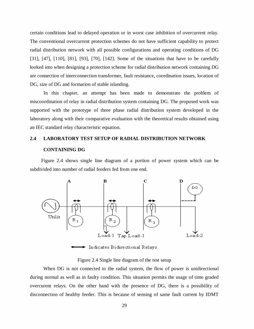
Figure 2.4 shows single line diagram of a portion of power system which can be
subdivided into number of radial feeders fed from one end.
Figure 2.4 Single line diagram of the test setup
When DG is not connected to the radial system, the flow of power is unidirectional
during normal as well as in faulty condition. This situation permits the usage of time graded
overcurent relays. On the other hand with the presence of DG, there is a possibility of
disconnection of healthy feeder. This is because of sensing of same fault current by IDMT
30
overcurrent relays (R2 & R3) for any downstream fault between substation C & D and for any
upstream fault between substation A & B of the radial distribution system.
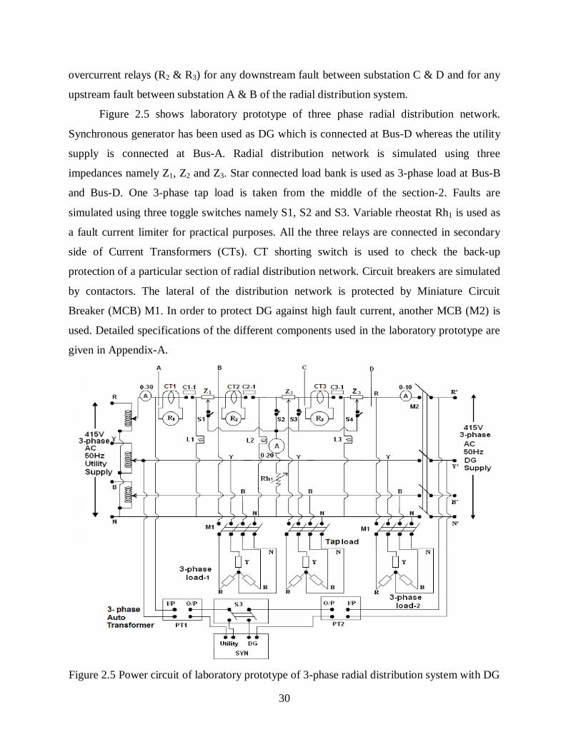
Figure 2.5 shows laboratory prototype of three phase radial distribution network.
Synchronous generator has been used as DG which is connected at Bus-D whereas the utility
supply is connected at Bus-A. Radial distribution network is simulated using three
impedances namely Z1, Z2 and Z3. Star connected load bank is used as 3-phase load at Bus-B
and Bus-D. One 3-phase tap load is taken from the middle of the section-2. Faults are
simulated using three toggle switches namely S1, S2 and S3. Variable rheostat Rh1 is used as
a fault current limiter for practical purposes. All the three relays are connected in secondary
side of Current Transformers (CTs). CT shorting switch is used to check the back-up
protection of a particular section of radial distribution network. Circuit breakers are simulated
by contactors. The lateral of the distribution network is protected by Miniature Circuit
Breaker (MCB) M1. In order to protect DG against high fault current, another MCB (M2) is
used. Detailed specifications of the different components used in the laboratory prototype are
given in Appendix-A.
Figure 2.5 Power circuit of laboratory prototype of 3-phase radial distribution system with DG
31
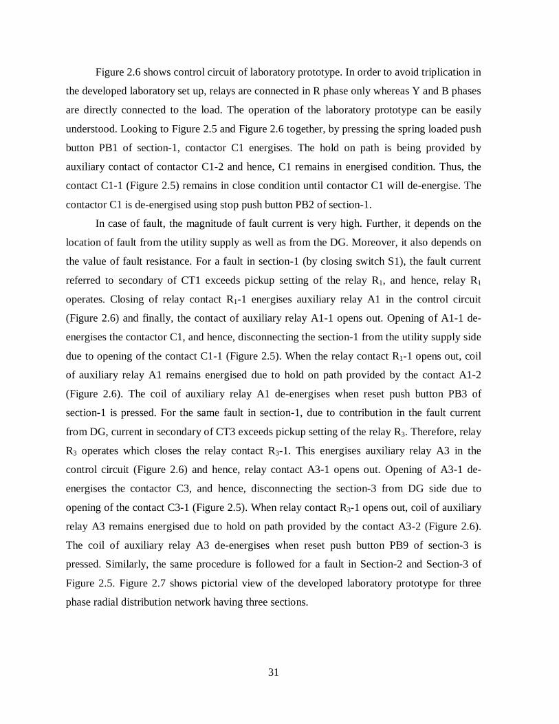
Figure 2.6 shows control circuit of laboratory prototype. In order to avoid triplication in
the developed laboratory set up, relays are connected in R phase only whereas Y and B phases
are directly connected to the load. The operation of the laboratory prototype can be easily
understood. Looking to Figure 2.5 and Figure 2.6 together, by pressing the spring loaded push
button PB1 of section-1, contactor C1 energises. The hold on path is being provided by
auxiliary contact of contactor C1-2 and hence, C1 remains in energised condition. Thus, the
contact C1-1 (Figure 2.5) remains in close condition until contactor C1 will de-energise. The
contactor C1 is de-energised using stop push button PB2 of section-1.
In case of fault, the magnitude of fault current is very high. Further, it depends on the
location of fault from the utility supply as well as from the DG. Moreover, it also depends on
the value of fault resistance. For a fault in section-1 (by closing switch S1), the fault current
referred to secondary of CT1 exceeds pickup setting of the relay R1, and hence, relay R1
operates. Closing of relay contact R1-1 energises auxiliary relay A1 in the control circuit
(Figure 2.6) and finally, the contact of auxiliary relay A1-1 opens out. Opening of A1-1 de-
energises the contactor C1, and hence, disconnecting the section-1 from the utility supply side
due to opening of the contact C1-1 (Figure 2.5). When the relay contact R1-1 opens out, coil
of auxiliary relay A1 remains energised due to hold on path provided by the contact A1-2
(Figure 2.6). The coil of auxiliary relay A1 de-energises when reset push button PB3 of
section-1 is pressed. For the same fault in section-1, due to contribution in the fault current
from DG, current in secondary of CT3 exceeds pickup setting of the relay R3. Therefore, relay
R3 operates which closes the relay contact R3-1. This energises auxiliary relay A3 in the
control circuit (Figure 2.6) and hence, relay contact A3-1 opens out. Opening of A3-1 de-
energises the contactor C3, and hence, disconnecting the section-3 from DG side due to
opening of the contact C3-1 (Figure 2.5). When relay contact R3-1 opens out, coil of auxiliary
relay A3 remains energised due to hold on path provided by the contact A3-2 (Figure 2.6).
The coil of auxiliary relay A3 de-energises when reset push button PB9 of section-3 is
pressed. Similarly, the same procedure is followed for a fault in Section-2 and Section-3 of
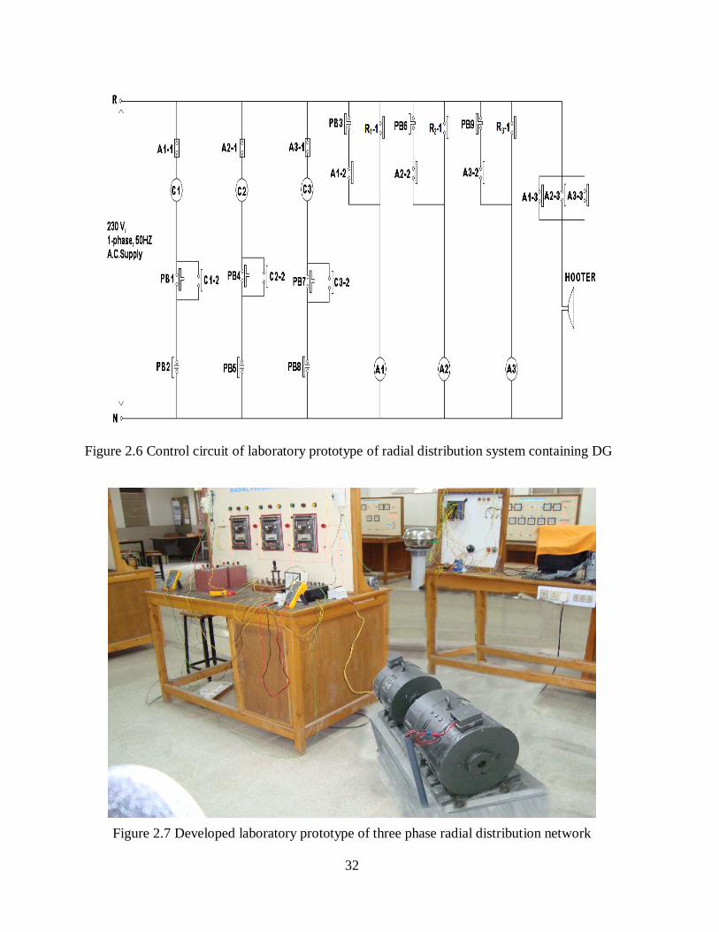
Figure 2.5. Figure 2.7 shows pictorial view of the developed laboratory prototype for three
phase radial distribution network having three sections.
32
Figure 2.6 Control circuit of laboratory prototype of radial distribution system containing DG
Figure 2.7 Developed laboratory prototype of three phase radial distribution network
33
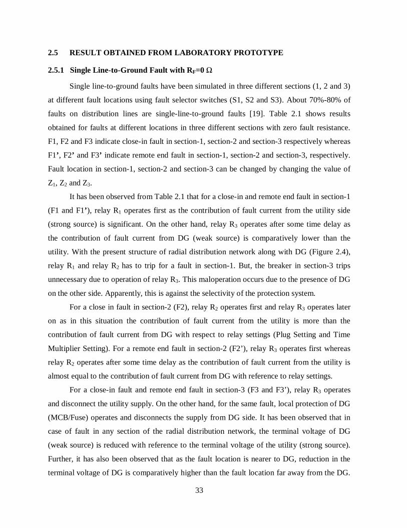
2.5 RESULT OBTAINED FROM LABORATORY PROTOTYPE
2.5.1 Single Line-to-Ground Fault with RF=0 Ω
Single line-to-ground faults have been simulated in three different sections (1, 2 and 3)
at different fault locations using fault selector switches (S1, S2 and S3). About 70%-80% of
faults on distribution lines are single-line-to-ground faults [19]. Table 2.1 shows results
obtained for faults at different locations in three different sections with zero fault resistance.
F1, F2 and F3 indicate close-in fault in section-1, section-2 and section-3 respectively whereas
F1’, F2’ and F3’ indicate remote end fault in section-1, section-2 and section-3, respectively.
Fault location in section-1, section-2 and section-3 can be changed by changing the value of
Z1, Z2 and Z3.
It has been observed from Table 2.1 that for a close-in and remote end fault in section-1
(F1 and F1’), relay R1 operates first as the contribution of fault current from the utility side
(strong source) is significant. On the other hand, relay R3 operates after some time delay as
the contribution of fault current from DG (weak source) is comparatively lower than the
utility. With the present structure of radial distribution network along with DG (Figure 2.4),
relay R1 and relay R2 has to trip for a fault in section-1. But, the breaker in section-3 trips
unnecessary due to operation of relay R3. This maloperation occurs due to the presence of DG
on the other side. Apparently, this is against the selectivity of the protection system.
For a close in fault in section-2 (F2), relay R2 operates first and relay R3 operates later
on as in this situation the contribution of fault current from the utility is more than the
contribution of fault current from DG with respect to relay settings (Plug Setting and Time
Multiplier Setting). For a remote end fault in section-2 (F2’), relay R3 operates first whereas
relay R2 operates after some time delay as the contribution of fault current from the utility is
almost equal to the contribution of fault current from DG with reference to relay settings.
For a close-in fault and remote end fault in section-3 (F3 and F3’), relay R3 operates
and disconnect the utility supply. On the other hand, for the same fault, local protection of DG
(MCB/Fuse) operates and disconnects the supply from DG side. It has been observed that in
case of fault in any section of the radial distribution network, the terminal voltage of DG
(weak source) is reduced with reference to the terminal voltage of the utility (strong source).
Further, it has also been observed that as the fault location is nearer to DG, reduction in the
terminal voltage of DG is comparatively higher than the fault location far away from the DG.

34
Hence, in case of fault on DG terminal (F3’), the utility will supply a small amount of fault
current due to the potential difference between the utility and DG.
2.5.2 Backup Protection
Backup protection is extremely important for any protection system if primary
protection system fails to clear the fault within its own zone of protection. Backup protection
feature has been tested for each section and the sample results for section-3 have been given in
Table 2.1-Table 2.4. The backup protection is simulated for section-3 using CT shorting
switch of CT3.
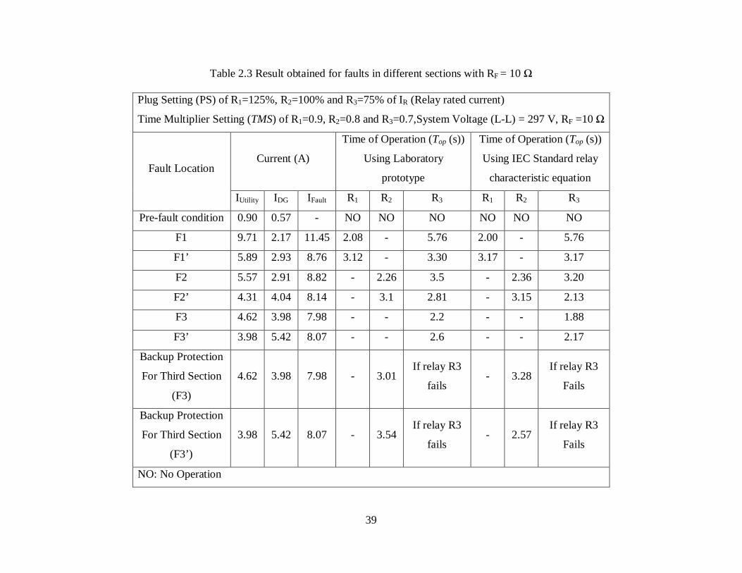
2.5.3 Effect of High Resistance Fault on Relays Coordination
When an overhead distribution phase conductor breaks and falls on a high impedance
surface or trees, high impedance fault occurs [14]. Due to insufficient magnitude of fault
current, the conventional overcurrent relays at the radial distribution network containing DG
may not be able to detect this type of fault and hence, relay does not operate. Table 2.2 to
Table 2.4 shows the results obtained for faults at different locations in all the three sections
with a variable fault resistance of 6 Ω, 10 Ω and 18 Ω, respectively.
The similar results, as obtained in Table 2.1, in terms of relay operation have been
observed for close-in and remote end fault in different sections with different values of fault
resistances. It has been observed from Table 2.2 - Table 2.4 that the time of operation of all
the relays increases as fault resistance increases. In certain conditions it is to be noted by the
authors that the relay may not be able to pickup due to a considerable value of fault resistance.
In case of backup protection, the backup relay does not operate if primary relay fails to
operate for a fault with RF > 20 Ω in its own zone.
2.6 RESULT OBTAINED FROM IEC STANDARD RELAY CHARACTERISTICS
EQUATION
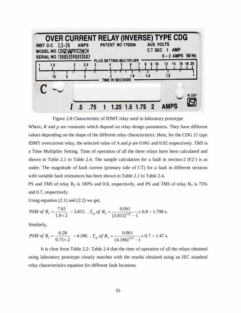
The characteristic of IDMT overcurrent relay is usually plotted between PSM and Top
of relay. The characteristic of IDMT relay used in prototype (CDG 21) has been shown in
Figure 2.8. Top of IDMT overcurrent relay is calculated using PSM and TMS. The standard
equations of PSM and Top for the above mentioned IDMT overcurrent relay are given in
equation (2.1) and (2.2).
35
Figure 2.8 Characteristic of IDMT relay used in laboratory prototype
Where, K and p are constants which depend on relay design parameters. They have different
values depending on the shape of the different relay characteristics. Here, for the CDG 21 type
IDMT overcurrent relay, the selected value of A and p are 0.061 and 0.02 respectively. TMS is
a Time Multiplier Setting. Time of operation of all the three relays have been calculated and
shown in Table 2.1 to Table 2.4. The sample calculation for a fault in section-2 (F2’) is as
under. The magnitude of fault current (primary side of CT) for a fault in different sections
with variable fault resistances has been shown in Table 2.1 to Table 2.4.
PS and TMS of relay R2 is 100% and 0.8, respectively, and PS and TMS of relay R3 is 75%
and 0.7, respectively.
Using equation (2.1) and (2.2) we get,
20.163.7
2 RofPSM = 3.815. , 8.0
1)815.3(061.0
02.02
RofTop = 1.798 s.
Similarly,
275.028.6
3 RofPSM = 4.186. , 7.0
1)186.4(061.0
02.03
RofTop = 1.47 s.
It is clear from Table 2.2- Table 2.4 that the time of operation of all the relays obtained
using laboratory prototype closely matches with the results obtained using an IEC standard
relay characteristics equation for different fault locations.

36
2.7 Conclusion
In the present chapter, a laboratory prototype of three phase radial distribution network
in the presence of DG has been presented. Miscoordination between relays has been studied
using the said prototype. It has been observed that for a fault in the nearest section from utility
side (section-1) with DG connected at the farthest bus (Bus-D), the relay situated in the next
to next substation (R3 in section-3) operates. In this situation, breaker of section-3 trips
unnecessarily and the continuity of power supply is affected in section-2 and section-3 which
is against the selectivity criteria of protection system. Further, the effect of high resistance
fault on relay operation has been analyzed for faults at different locations in different line
sections. It has been observed that the possibility of operation of IDMT overcurrent relays
reduces as the value of fault resistance increases. Moreover, the performance of the
conventional IDMT overcurrent relays has been checked during back-up protection if primary
protection system fails to operate for a fault within its own zone. The time of operations of all
the relays of radial distribution network obtained from the developed laboratory prototype for
different fault locations in various sections have been found to be in close conformity with the
theoretical values obtained using an IEC standard relay characteristics equation.
37
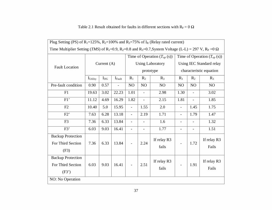
Table 2.1 Result obtained for faults in different sections with RF = 0 Ω
Plug Setting (PS) of R1=125%, R2=100% and R3=75% of IR (Relay rated current)
Time Multiplier Setting (TMS) of R1=0.9, R2=0.8 and R3=0.7,System Voltage (L-L) = 297 V, RF =0 Ω
Fault Location Current (A)
Time of Operation (Top (s))
Using Laboratory
prototype
Time of Operation (Top (s))
Using IEC Standard relay
characteristic equation
IUtility IDG IFault R1 R2 R3 R1 R2 R3
Pre-fault condition 0.90 0.57 - NO NO NO NO NO NO
F1 19.63 3.02 22.23 1.01 - 2.98 1.30 - 3.02
F1’ 11.12 4.69 16.29 1.82 - 2.15 1.81 - 1.85
F2 10.40 5.0 15.95 - 1.55 2.0 - 1.45 1.75
F2’ 7.63 6.28 13.18 - 2.19 1.71 - 1.79 1.47
F3 7.36 6.33 13.84 - - 1.6 - - 1.32
F3’ 6.03 9.03 16.41 - - 1.77 - - 1.51
Backup Protection
For Third Section
(F3)
7.36 6.33 13.84 - 2.24 If relay R3
fails - 1.72
If relay R3
Fails
Backup Protection
For Third Section
(F3’)
6.03 9.03 16.41 - 2.51 If relay R3
fails - 1.91
If relay R3
Fails
NO: No Operation
38
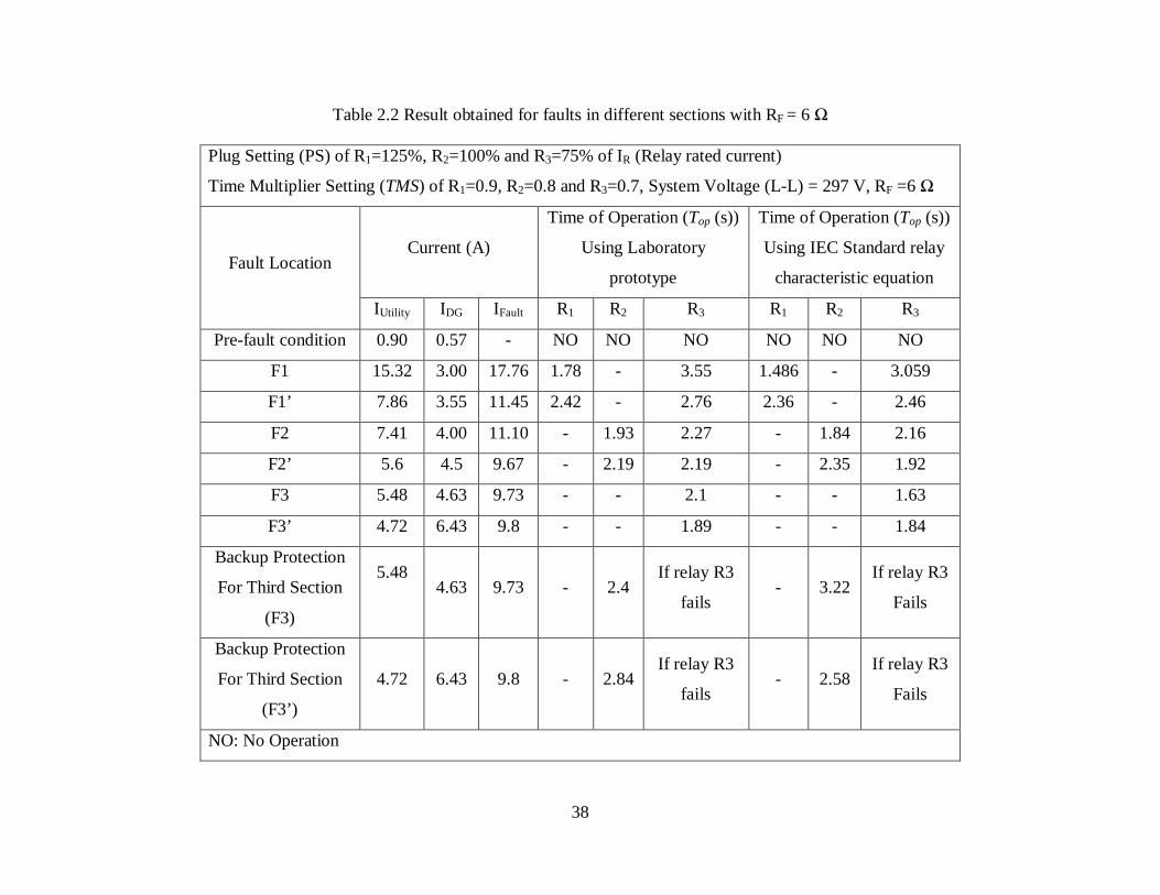
Table 2.2 Result obtained for faults in different sections with RF = 6 Ω
Plug Setting (PS) of R1=125%, R2=100% and R3=75% of IR (Relay rated current)
Time Multiplier Setting (TMS) of R1=0.9, R2=0.8 and R3=0.7, System Voltage (L-L) = 297 V, RF =6 Ω
Fault Location Current (A)
Time of Operation (Top (s))
Using Laboratory
prototype
Time of Operation (Top (s))
Using IEC Standard relay
characteristic equation
IUtility IDG IFault R1 R2 R3 R1 R2 R3
Pre-fault condition 0.90 0.57 - NO NO NO NO NO NO
F1 15.32 3.00 17.76 1.78 - 3.55 1.486 - 3.059
F1’ 7.86 3.55 11.45 2.42 - 2.76 2.36 - 2.46
F2 7.41 4.00 11.10 - 1.93 2.27 - 1.84 2.16
F2’ 5.6 4.5 9.67 - 2.19 2.19 - 2.35 1.92
F3 5.48 4.63 9.73 - - 2.1 - - 1.63
F3’ 4.72 6.43 9.8 - - 1.89 - - 1.84
Backup Protection
For Third Section
(F3)
5.48
4.63 9.73 - 2.4
If relay R3
fails - 3.22
If relay R3
Fails
Backup Protection
For Third Section
(F3’)
4.72 6.43 9.8 - 2.84 If relay R3
fails - 2.58
If relay R3
Fails
NO: No Operation
39
Table 2.3 Result obtained for faults in different sections with RF = 10 Ω
Plug Setting (PS) of R1=125%, R2=100% and R3=75% of IR (Relay rated current)
Time Multiplier Setting (TMS) of R1=0.9, R2=0.8 and R3=0.7,System Voltage (L-L) = 297 V, RF =10 Ω
Fault Location Current (A)
Time of Operation (Top (s))
Using Laboratory
prototype
Time of Operation (Top (s))
Using IEC Standard relay
characteristic equation
IUtility IDG IFault R1 R2 R3 R1 R2 R3
Pre-fault condition 0.90 0.57 - NO NO NO NO NO NO
F1 9.71 2.17 11.45 2.08 - 5.76 2.00 - 5.76
F1’ 5.89 2.93 8.76 3.12 - 3.30 3.17 - 3.17
F2 5.57 2.91 8.82 - 2.26 3.5 - 2.36 3.20
F2’ 4.31 4.04 8.14 - 3.1 2.81 - 3.15 2.13
F3 4.62 3.98 7.98 - - 2.2 - - 1.88
F3’ 3.98 5.42 8.07 - - 2.6 - - 2.17
Backup Protection
For Third Section
(F3)
4.62 3.98 7.98 - 3.01 If relay R3
fails - 3.28
If relay R3
Fails
Backup Protection
For Third Section
(F3’)
3.98 5.42 8.07 - 3.54 If relay R3
fails - 2.57
If relay R3
Fails
NO: No Operation

40
Table 2.4 Result obtained for faults in different sections with RF = 18 Ω
Plug Setting (PS) of R1=125%, R2=100% and R3=75% of IR (Relay rated current)
Time Multiplier Setting (TMS) of R1=0.9, R2=0.8 and R3=0.7, System Voltage (L-L) = 297 V, RF =18 Ω
Fault Location Current (A)
Time of Operation (Top (s))
Using Laboratory
prototype
Time of Operation (Top (s))
Using IEC Standard relay
characteristic equation
IUtility IDG IFault R1 R2 R3 R1 R2 R3
Pre-fault condition 0.90 0.57 - NO NO NO NO NO NO
F1 5.59 1.75 6.63 3.3 - 14.20 3.38 - 13.83
F1’ 4.05 2.1 5.63 5.78 - 6.98 5.66 - 6.32
F2 3.81 2.4 5.58 - 3.49 5.96 - 3.76 4.52
F2’ 3.04 3.98 5.28 - 6.41 3.15 - 5.80 2.17
F3 2.65 3.96 5.34 - - 4.77 - - 3.73
F3’ 2.51 4.56 5.65 - - 5.28 - - 4.13
Backup Protection
For Third Section
(F3)
2.65 3.96 5.34 - 5.34
If relay R3
fails - 4.13
If relay R3
Fails
Backup Protection
For Third Section
(F3’)
2.51 4.56 5.65 - 8.12 If relay R3
fails - 4.53
If relay R3
Fails
NO: No Operation