Chapter 2 FOUNDAMENTAL CONCEPTS 2.1 Fluid as a Continuum We are all familiar with fluids—the most common being air

and water—and we experience them as being “smooth,” i.e., as being a continuous medium. Unless we use specialized equipment, we are not aware of the underlying molecular nature of fluids. This molecular structure is one in which the mass is not

continuously distributed in space, but is concentrated in molecules that are separated by relatively large regions of empty space.

A region of space “filled” by a stationary fluid (e.g., air, treated

as a single gas) looks like a continuous medium, but if we zoom in on a very small cube of it, we can see that we mostly have empty space, with gas molecules scattered around, moving at high speed (indicated by the gas temperature).

We wish to ask: What is the minimum volume, V , that a “point” C must be, so that we can talk about continuous fluid properties such as the density at a point? In other words, under what circumstances can a fluid be treated as a continuum, for which, by definition, properties vary smoothly from point to point? This is an important question because the concept of a

continuum is the basis of classical fluid mechanics. Consider how we determine the density at a point. Density is

defined as mass per unit volume. The mass δm will be given by the instantaneous number of molecules in V (and the mass of each molecule), so the average density in volume V is given by /m V . We say “average” because the number of molecules in V ,

and hence the density, fluctuates. For example, if the gas was air at standard temperature and

pressure (STP) and the volume was a sphere of diameter 0.01 μm, there might be 15 molecules in V , but an instant later there might be 17 (three might enter while one leaves). Hence the density at “point” C randomly fluctuates in time. In this figure, each vertical dashed line represents a specific

chosen volume, V , and each data point represents the measured density at an instant. For very small volumes, the density varies greatly, but above a certain volume, V , the density becomes stable—the volume now encloses a huge number of molecules. For example, if V =0.001 mm3 (about the size of a grain of

sand), there will on average be 2.51013 molecules present.

Hence we can conclude that air at STP (and other gases, and liquids) can be treated as a continuous medium as long as we consider a“point” to be no smaller than about this size; this is

sufficiently precise for most engineering applications. The concept of a continuum is the basis of classical fluid

mechanics. The continuum assumption is valid in treating the behavior of fluids under normal conditions. It only breaks down when the mean free path of the molecules (~610-8 m at STP) becomes the same order of magnitude as the smallest significant characteristic dimension of the problem. This occurs in such specialized problems as rarefied gas flow

(e.g., as encountered in flights into the upper reaches of the atmosphere). For these specialized cases (not covered in this

text) we must abandon the concept of a continuum in favor of the microscopic and statistical points of view. As a consequence of the continuum assumption, each fluid

property is assumed to have a definite value at every point in space. Thus fluid properties such as density, temperature, velocity, and so on are considered to be continuous functions of position and time. For example, we now have a workable definition of density at

a point,

limV V

mV

Since point C was arbitrary, the density at any other point in the fluid could be determined in the same manner. If density was measured simultaneously at an infinite number

of points in the fluid, we would obtain an expression for the density distribution as a function of the space coordinates, ρ=ρ(x, y, z), at the given instant. The density at a point may also vary with time (as a result of

work done on or by the fluid and/or heat transfer to the fluid). Thus the complete representation of density (the field representation) is given by ρ=ρ(x, y, z, t). Since density is a scalar quantity, requiring only the

specification of a magnitude for a complete description, the field represented by above equation is a scalar field. An alternative way of expressing the density of a substance

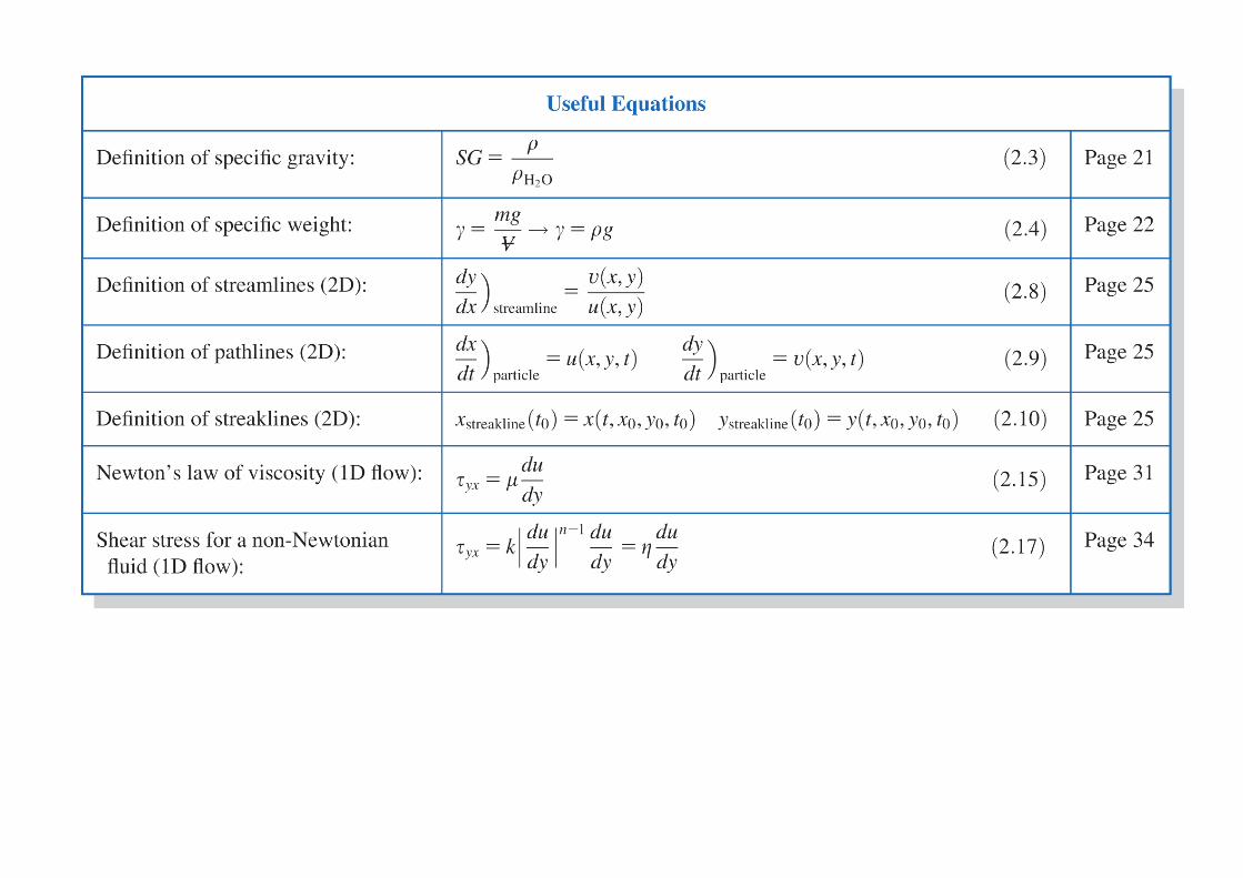
(solid or fluid) is to compare it to an accepted reference value, typically the maximum density of water,

2H O (1000 kg/m3 at

�4 C or 1.94 slug/ft3 �at 39 F). Thus, the specific gravity, SG,

of a substance is expressed as 2H O

SG

.

For example, the SG of mercury is typically 13.6—mercury is 13.6 times as dense as water. Appendix A contains specific gravity data for selected engineering materials. The specific gravity of liquids is a function of temperature; for

most liquids specific gravity decreases with increasing temperature. The specific weight, γ, of a substance is another useful

material property. It is defined as the weight of a substance per

unit volume and given as mg gV

.

For example, the specific weight of water is approximately 9.81 kN/m3 (62.4 lbf/ft3).

2.2 Velocity Field In the previous section we saw that the continuum assumption

led directly to the notion of the density field. Other fluid properties also may be described by fields. A very important property defined by a field is the velocity field, given by

( , , , )V V x y z t

. Velocity is a vector quantity, requiring a magnitude and

direction for a complete description, so the velocity field is a vector field. The velocity vector, V

, also can be written in terms of its

three scalar components. Denoting the components in the x, y, and z directions by u, v, and w, then V ui vj wk

In general, each component, u, v, and w, will be a function of x, y, z, and t. We need to be clear on what ( , , , )V V x y z t

measures: It

indicates the velocity of a fluid particle that is passing through the point x, y, z at time instant t, in the Eulerian sense. We can keep measuring the velocity at the same point or

choose any other point x, y, z at the next time instant; the point x, y, z is not the ongoing position of an individual particle, but a point we choose to look at. (Hence x, y, and z are independent variables.

We conclude that ( , , , )V V x y z t

should be thought of as the velocity field of all particles, not just the velocity of an individual particle. If properties at every point in a flow field do not change with

time, the flow is termed steady. Stated mathematically, the definition of steady flow is

0t

where η represents any fluid property. Hence, for steady flow,

0 or ( , , ) and 0 or ( , , )Vx y z V V x y zt t

In steady flow, any property may vary from point to point in the field, but all properties remain constant with time at every

point One-, Two-, and Three Dimensional Flows A flow is classified as one-, two-, or three-dimensional

depending on the number of space coordinates required to specify the velocity field. Although most flow fields are inherently three-dimensional,

analysis based on fewer dimensions is frequently meaningful. Consider, for example, the steady flow through a long

straight pipe that has a divergent section.

In this example, we are using cylindrical coordinates (r, θ, x).

We will learn (in Chapter 8) that under certain circumstances (e.g., far from the entrance of the pipe and from the divergent section, where the flow can be quite complicated), the velocity distribution may be described by

2

max 1 ru uR

This is shown on the left of following figure. The velocity

u(r) is a function of only one coordinate, and so the flow is one-dimensional. On the other hand, in the diverging section, the velocity

decreases in the x direction, and the flow becomes two-dimensional: u=u(r, x). As you might suspect, the complexity of analysis increases

considerably with the number of dimensions of the flow field. For many problems encountered in engineering, a one-dimensional analysis is adequate to provide approximate solutions of engineering accuracy. Since all fluids satisfying the continuum assumption must

have zero relative velocity at a solid surface (to satisfy the no-slip condition), most flows are inherently two or three-dimensional.

To simplify the analysis it is often convenient to use the notion of uniform flow at a given cross section. In a flow that is uniform at a given cross section, the velocity is constant across any section normal to the flow. Under this assumption, the two-dimensional flow is modeled as the flow shown in following figure.

In the flow of above figure, the velocity field is a function of

x alone, and thus the flow model is one-dimensional. (Other properties, such as density or pressure, also may be assumed

uniform at a section, if appropriate.) The term uniform flow field (as opposed to uniform flow at

a cross section) is used to describe a flow in which the velocity is constant, i.e., independent of all space coordinates, throughout the entire flow field.

Timelines, Pathlines, Streaklines, and Streamlines Airplane and auto companies and college engineering

laboratories, among others, frequently use wind tunnels to visualize flow fields. For example, the following figure shows a flow pattern for

flow around a car mounted in a wind tunnel, generated by releasing smoke into the flow at five fixed upstream points.

Flow patterns can be visualized using timelines, pathlines, streaklines, or streamlines. If a number of adjacent fluid particles in a flow field are

marked at a given instant, they form a line in the fluid at that instant; this line is called a timeline. Subsequent observations of the line may provide information about the flow field. For example, in discussing the behavior of a fluid under the action of a constant shear force (Section 1.2) timelines were introduced to demonstrate the deformation of a fluid at successive instants.

A pathline is the path or trajectory traced out by a moving

fluid particle. To make a pathline visible, we might identify a fluid particle at a given instant, e.g., by the use of dye or smoke, and then take a long exposure photograph of its subsequent motion. The line traced out by the particle is a pathline. This approach might be used to study, for example,

the trajectory of a contaminant leaving a smokestack.

On the other hand, we might choose to focus our attention

on a fixed location in space and identify, again by the use of dye or smoke, all fluid particles passing through this point. After a short period of time we would have a number of identifiable fluid particles in the flow, all of which had, at some time, passed through one fixed location in space. The

line joining these fluid particles is defined as a streakline.

Streamlines are lines drawn in the flow field so that at a

given instant they are tangent to the direction of flow at

every point in the flow field. Since the streamlines are tangent to the velocity vector at every point in the flow field, there can be no flow across a streamline. Streamlines are the most commonly used visualization technique.

In steady flow, the velocity at each point in the flow field

remains constant with time and, consequently, the streamline shapes do not vary from one instant to the next. This implies that a particle located on a given streamline will always move along the same streamline. Furthermore, consecutive particles passing through a fixed point in space will be on the same streamline and, subsequently, will remain on this streamline. Thus in a steady flow, pathlines, streaklines, and streamlines are identical lines in the flow field. We can also define streamlines. These are lines drawn in the

flow field so that at a given instant they are tangent to the direction of flow at every point in the flow field. Since the streamlines are tangent to the velocity vector at every point in the flow field, there is no flow across a streamline. Pathlines are as the name implies: They show, over time, the

paths individual particles take (if you’ve seen time-lapse photos of nighttime traffic, you get the idea). Finally, timelines are created by marking a line in a flow and

watching how it evolves over time. We conclude that for steady flow, streaklines, streamlines,

and pathlines are identical. Things are quite different for unsteady flow. For unsteady

flow, streaklines, streamlines, and pathlines will in general have differing shapes. For example, consider holding a garden hose and swinging it

side to side as water exits at high speed, as shown in the following figure. We obtain a continuous sheet of water. If we consider individual water particles, we see that each particle, once ejected, follows a straight-line path (here, for

simplicity, we ignore gravity): The pathlines are straight lines, as shown.

On the other hand, if we start injecting dye into the water as

it exits the hose, we will generate a streakline, and this takes the shape of an expanding sine wave, as shown.

Clearly, pathlines and streaklines do not coincide for this unsteady flow (we leave determination of streamlines to an exercise). We can use the velocity field to derive the shapes of

streaklines, pathlines, and streamlines. Starting with streamlines: Because the streamlines are

parallel to the velocity vector, we can write (for 2D)

streamline

( , )( , )

dy v x ydx u x y

Note that streamlines are obtained at an instant in time; if the flow is unsteady, time t is held constant in the above equation. Solution of this equation gives the equation y=y(x), with an undetermined integration constant, the value of

which determines the particular streamline. For pathlines (again considering 2D), we let x=xp and y= yp,

where xp(t) and yp(t) are the instantaneous coordinates of a specific particle. We then get

particle particle

( , , ), ( , , )dx dyu x y t v x y tdt dt

The simultaneous solution of these equations gives the path of a particle in parametric form xp(t), yp(t). The computation of streaklines is somewhat tricky. The first

step is to compute the pathline of a particle (using the above equation) that was released from the streak source point (coordinates x0, y0) at time t0, in the form

particle 0 0 0 particle 0 0 0( ) ( , , , ), ( ) ( , , , )x t x t x y t y t x t x y t

Then, instead of interpreting this as the position of a particle over time, we rewrite these equations as

streakline 0 0 0 0 streakline 0 0 0 0( ) ( , , , ), ( ) ( , , , )x t x t x y t y t x t x y t Above equations give the line generated (by time t) from a

streak source at point (x0, y0). In these equations, t0 (the release times of particles) is varied from 0 to t to show the instantaneous positions of all particles released up to time t!

Ex. 2.1 Streamlines and pathlines in two-dimensional flow: A velocity field is given byV Axi Ayj

; the units of velocity are

m/s; x and y are given in meters; A=0.3 s-1.(a) Obtain an equation for the streamlines in the xy plane.(b) Plot the streamline passing through the point (x0, y0)=(2, 8).(c) Determine the velocity of a

particle at the point (2, 8).(d) If the particle passing through the point (x0, y0) is marked at time t=0, determine the location of the particle at time t=6 s.(e) What is the velocity of this particle at time t=6 s?(f) Show that the equation of the particle path (the pathline) is the same as the equation of the streamline. Given: Velocity field, V Axi Ayj

; x and y in meters; A=0.3 s-1.

Find: (a) Equation of the streamlines in the xy plane.(b) Streamline plot through point (2, 8).(c) Velocity of particle at point (2, 8).(d) Position at t=6 s of particle located at (2, 8) at t=0.(e) Velocity of particle at position found in (d).(f) Equation of pathline of particle located at (2, 8) at t=0.

Notes: # This problem illustrates the method for computing

streamlines and pathlines. # Because this is a steady flow, the streamlines and pathlines have the same shape—in an unsteady flow this would not be true. # When we follow a particle (the Lagrangian approach), its position (x, y) and velocity (up=dx/dt and vp=dy/dt) are functions of time, even though the flow is steady.

2.3 Stress Field In our study of fluid mechanics, we will need to understand

what kinds of forces act on fluid particles. Each fluid particle can experience: surface forces (pressure,

friction) that are generated by contact with other particles or a solid surface; and body forces (such as gravity and electromagnetic) that are experienced throughout the particle. The gravitational body force acting on an element of volume,

dV , is given by gdV , where ρ is the density (mass per unit volume) and g is the local gravitational acceleration. Thus the gravitational body force per unit volume is g and the gravitational body force per unit mass is g . Surface forces on a fluid particle lead to stresses. The concept

of stress is useful for describing how forces acting on the

boundaries of a medium (fluid or solid) are transmitted throughout the medium. You have probably seen stresses discussed in solid mechanics. For example, when you stand on a diving board, stresses are

generated within the board. On the other hand, when a body moves through a fluid, stresses are developed within the fluid. The difference between a fluid and a solid is, as we’ve seen, that stresses in a fluid are mostly generated by motion rather than by deflection. Imagine the surface of a fluid particle in contact with other

fluid particles, and consider the contact force being generated between the particles. Consider a portion, A

, of the surface

at some point C. The orientation of A

is given by the unit vector, n . The vector n is the outwardly drawn unit normal

with respect to the particle.

The force, F

, acting on A

may be resolved into two

components, one normal to and the other tangent to the area. A normal stress σn and a shear stress τn are then defined as

0 0lim and lim

n n

n tn nA A

n n

F FA A

Subscript n on the stress is included as a reminder that the stresses are associated with the surface A

through C, having

an outward normal in the n direction. The fluid is actually a continuum, so we could have imagined

breaking it up any number of different ways into fluid particles around point C, and therefore obtained any number of different stresses at point C. In dealing with vector quantities such as force, we usually

consider components in an orthogonal coordinate system. In rectangular coordinates we might consider the stresses acting on planes whose outwardly drawn normals (again with respect to the material acted upon) are in the x, y, or z directions.

In the above figures we consider the stress on the element δAx,

whose outwardly drawn normal is in the x direction. The force, F

, has been resolved into components along each of the coordinate directions. Dividing the magnitude of each force component by the area, δAx, and taking the limit as δAx

approaches zero, we define the three stress components shown in the above figure:

0 0 0lim , lim , lim

x x x

yx zxx xy xzA A A

x x x

FF FA A A

We have used a double subscript notation to label the stresses. The first subscript (in this case, x) indicates the plane on which the stress acts (in this case, a surface perpendicular to the x axis). The second subscript indicates the direction in which the stress acts. Consideration of area element δAy would lead to the

definitions of the stresses, σyy, yx, and τyz; use of area element δAz would similarly lead to the definitions of σzz, τzx, τzy. Although we just looked at three orthogonal planes, an infinite

number of planes can be passed through point C, resulting in an infinite number of stresses associated with planes through

that point. Fortunately, the state of stress at a point can be described

completely by specifying the stresses acting on any three mutually perpendicular planes through the point. The stress at a point is specified by the nine components

xx xy xz

yx yy yz

zx zy zz

where σ has been used to denote a normal stress, and τ to denote a shear stress. The notation for designating stress is shown in the following

figure.

2.4 Viscosity Where do stresses come from? For a solid, stresses develop

when the material is elastically deformed or strained; for a

fluid, shear stresses arise due to viscous flow (we will discuss a fluid’s normal stresses shortly). Hence we say solids are elastic, and fluids are viscous (and it’s interesting to note that many biological tissues are viscoelastic, meaning they combine features of a solid and a fluid). For a fluid at rest, there will be no shear stresses. We will see

that each fluid can be categorized by examining the relation between the applied shear stresses and the flow (specifically the rate of deformation) of the fluid. Consider the behavior of a fluid element between the two

infinite plates shown in the following figure. The rectangular fluid element is initially at rest at time t. Let us now suppose a constant rightward force δFx is applied to the upper plate so that it is dragged across the fluid at constant velocity δu. The

relative shearing action of the infinite plates produces a shear stress, τyx, which acts on the fluid element and is given by

0lim

y

x xyx A

y y

F dFA dA

where δAy is the area of contact of the fluid element with the plate and δFx is the force exerted by the plate on that element.

Snapshots of the fluid element illustrate the deformation of the

fluid element from position MNOP at time t, to M’NOP’ at time

t+δt, to M”NOP” at time t+2δt, due to the imposed shear stress. As mentioned in Section 1.2, it is the fact that a fluid

continually deforms in response to an applied shear stress that sets it apart from solids. Focusing on the time interval δt, the deformation of the fluid is

given by

0deformation rate lim

t

dt dt

We want to express dα/dt in terms of readily measurable quantities. This can be done easily. The distance, δl, between the points M and M’ is given by

l u t Alternatively, for small angles,

l y

Equating these two expressions for δl gives u

t y

Taking the limits of both sides of the equality, we obtain d dudt dy

Thus, the fluid element when subjected to shear stress τyx, experiences a rate of deformation (shear rate) given by du/dy. We have established that any fluid that experiences a shear stress will flow (it will have a shear rate). What is the relation between shear stress and shear rate? Fluids

in which shear stress is directly proportional to rate of deformation are Newtonian fluids. The term non-Newtonian is used to classify all fluids in which shear stress is not directly

proportional to shear rate.

Newtonian Fluid Most common fluids (the ones discussed in this text) such as

water, air, and gasoline are Newtonian under normal conditions. If the fluid is Newtonian, then

yxdudy

We are familiar with the fact that some fluids resist motion more than others. For example, a container of SAE 30W oil is much harder to

stir than one of water. Hence SAE 30W oil is much more viscous—it has a higher viscosity. The constant of proportionality in the above equation is the

absolute (or dynamic) viscosity, μ. Thus in terms of the coordinates shown in the figure, Newton’s law of viscosity is given for one-dimensional flow by

yxdudy

Note that, since the dimensions of τ are [F/L2] and the dimensions of du/dy are [1/t], μ has dimensions [Ft/L2]. Since the dimensions of force, F, mass, M, length, L, and time, t, are related by Newton’s second law of motion, the dimensions of μ can also be expressed as [M/Lt]. In the British Gravitational system, the units of viscosity are lbf·s/ft2 or slug/(ft·s). In the

Absolute Metric system, the basic unit of viscosity is called a poise [1 poise1 g/(cm·s)]; in the SI system the units of

viscosity are kg/(m·s) or Pa·s (1 Pa·s1 N·s/m2). In fluid mechanics the ratio of absolute viscosity, μ, to density, ρ, often arises. This ratio is given the name kinematic viscosity and is represented by the symbol ν. Since density has dimensions [M/L3], the dimensions of ν are [L2/t]. In the Absolute Metric system of units, the unit for ν is a stoke (1 stoke1 cm2/s) ; in the SI system of units, the unit for ν is m2/s. Viscosity data for a number of common Newtonian fluids are

given in Appendix A. Note that for gases, viscosity increases with temperature,

whereas for liquids, viscosity decreases with increasing temperature.

Ex. 2.2 Viscosity and shear stress in Newtonian Fluid: An

infinite plate is moved over a second plate on a layer of liquid as shown. For small gap width, d, we assume a linear velocity distribution in the liquid. The liquid viscosity is 0.0065 g/cm·s and its specific gravity is 0.88. Determine:(a) The absolute viscosity of the liquid, in N·s/m2.(b) The kinematic viscosity of the liquid, in m2/s.(c) The shear stress on the upper plate, in N/m2.(d) The shear stress on the lower plate, in Pa.(e) The direction of each shear stress calculated in parts (c) and (d). Given: Linear velocity profile, =0.0065 g/cm·s, SG=0.88 Find: (a) μ in units of N·s/m2.(b) ν in units of m2/s.(c) on upper plate in units of N/m2.(d) on lower plate in units of Pa.(e) Direction of stresses in parts (c) and (d).

Part (c) shows that the shear stress is: # Constant across the gap

for a linear velocity profile. # Directly proportional to the speed of the upper plate (because of the linearity of Newtonian fluids). # Inversely proportional to the gap between the plates. Note that multiplying the shear stress by the plate area in such problems computes the force required to maintain the motion. Non-Newtonian Fluid Fluids in which shear stress is not directly proportional to

deformation rate are non-Newtonian. Although we will not discuss these much in this text, many

common fluids exhibit non-Newtonian behavior. Two familiar examples are toothpaste and Lucite paint. The latter is very “thick” when in the can, but becomes “thin” when sheared by brushing. Toothpaste behaves as a “fluid” when squeezed from the tube. However, it does not run out by itself when the cap is removed. There is a threshold or yield stress below which toothpaste behaves as a solid. Strictly speaking, our definition of a fluid is valid only for materials that have zero yield stress. Non-Newtonian fluids commonly are classified as having

time-independent or time-dependent behavior. Examples of time-independent behavior are shown in the

following rheological diagram.

Numerous empirical equations have been proposed to model

the observed relations between τyx and du/dy for time-independent fluids. They may be adequately represented for many engineering applications by the power law model, which for one-dimensional flow becomes

n

yxdukdy

where the exponent, n, is called the flow behavior index and the coefficient, k, the consistency index. This equation reduces to Newton’s law of viscosity for n=1 with k=μ. To ensure that τyx has the same sign as du/dy, the above

equation is rewritten in the form 1n

yxdu du dukdy dy dy

The term 1/ nk du dy is referred to as the apparent viscosity. The idea behind the above equation is that we end up with a viscosity η that is used in a formula that is the same form as /yx du dy , in which the Newtonian viscosity μ is

used. The big difference is that while μ is constant (except for temperature effects), η depends on the shear rate. Most non-Newtonian fluids have apparent viscosities that are

relatively high compared with the viscosity of water. Fluids in which the apparent viscosity decreases with

increasing deformation rate (n<1) are called pseudoplastic (or shear thinning) fluids. Most non-Newtonian fluids fall into this group; examples include polymer solutions, colloidal suspensions, and paper pulp in water.

If the apparent viscosity increases with increasing deformation rate (n>1) the fluid is termed dilatant (or shear thickening). Suspensions of starch and of sand are examples of dilatant fluids. You can get an idea of the latter when you’re on the beach—if you walk slowly (and hence generate a low shear rate) on very wet sand, you sink into it, but if you jog on it (generating a high shear rate), it’s very firm. A “fluid” that behaves as a solid until a minimum yield stress, τy, is exceeded and subsequently exhibits a linear relation between stress and rate of deformation is referred to as an ideal or Bingham plastic. The corresponding shear stress model is

/yx y pdu dy

Clay suspensions, drilling muds, and toothpaste are examples of substances exhibiting this behavior. The study of non-Newtonian fluids is further complicated by

the fact that the apparent viscosity may be time-dependent. Thixotropic fluids show a decrease in η with time under a

constant applied shear stress; many paints are thixotropic. Rheopectic fluids show an increase in η with time. After

deformation some fluids partially return to their original shape when the applied stress is released; such fluids are called viscoelastic (many biological fluids work this way).

2.5 Surface Tension You can tell when your car needs waxing: Water droplets tend

to appear somewhat flattened out. After waxing, you get a nice

“beading” effect.

We define a liquid as “wetting” a surface when the contact

angle θ< 90. By this definition, the car’s surface was wetted before waxing,

and not wetted after. This is an example of effects due to surface tension. Whenever a liquid is in contact with other liquids or gases, or in this case a gas/solid surface, an interface develops that acts like a stretched elastic membrane, creating

surface tension. There are two features to this membrane: the contact angle, θ,

and the magnitude of the surface tension, σ (N/m or lbf/ft). Both of these depend on the type of liquid and the type of solid surface (or other liquid or gas) with which it shares an interface. In the car-waxing example, the contact angle changed from

being smaller than 90, to larger than 90, because, in effect, the waxing changed the nature of the solid surface. Factors that affect the contact angle include the cleanliness of the surface and the purity of the liquid. Other examples of surface tension effects arise when you are

able to place a needle on a water surface and, similarly, when small water insects are able to walk on the surface of the water. Appendix A contains data for surface tension and contact angle

for common liquids in the presence of air and of water. A force balance on a segment of interface shows that there is a

pressure jump across the imagined elastic membrane whenever the interface is curved. For a water droplet in air, pressure in the water is higher than ambient; the same is true for a gas bubble in liquid. For a soap bubble in air, surface tension acts on both inside and outside interfaces between the soap film and air along the curved bubble surface. Surface tension also leads to the phenomena of capillary (i.e.,

very small wavelength) waves on a liquid surface, and capillary rise or depression. In engineering, probably the most important effect of surface

tension is the creation of a curved meniscus that appears in manometers or barometers, leading to a (usually unwanted)

capillary rise (or depression). This rise may be pronounced if the liquid is in a small-diameter tube or narrow gap.

Ex. 2.3 Analysis of capillary effect in a tube: Create a graph showing the capillary rise or fall of a column of water or mercury,

respectively, as a function of tube diameter D. Find the minimum diameter of each column required so that the height magnitude will be less than 1 mm. Given: Tube dipped in liquid as in the following figure. Find: A general expression for Δh as a function of D.

This problem: # reviewed use of the free-body diagram approach. # It turns out that neglecting the volume in the meniscus region is only valid when Δh is large compared with D. However, in this problem we have the result that Δh is

about 1 mm when D is 11.2 mm (or 30 mm); hence the results can only be very approximate. Folsom (1937) shows that the simple analysis of Example 2.3

overpredicts the capillary effect and gives reasonable results only for tube diameters less than 2.54 mm. Over a diameter range 2.54<D<27.94 mm, experimental data for the capillary rise with a water-air interface are correlated by the empirical expression Δh=0.400/e4.37D. Manometer and barometer readings should be made at the level

of the middle of the meniscus. This is away from the maximum effects of surface tension and thus nearest to the proper liquid level. All surface tension data in Appendix A were measured for pure

liquids in contact with clean vertical surfaces. Impurities in the liquid, dirt on the surface, or surface inclination can cause an indistinct meniscus; under such conditions it may be difficult to determine liquid level accurately. Liquid level is most distinct in a vertical tube. When inclined

tubes are used to increase manometer sensitivity (see Section 3.3) it is important to make each reading at the same point on the meniscus and to avoid use of tubes inclined less than about 15 from horizontal. Surfactant compounds reduce surface tension significantly

(more than 40% with little change in other properties) when added to water. They have wide commercial application: Most detergents contain surfactants to help water penetrate and lift soil from surfaces. Surfactants also have major industrial applications in catalysis, aerosols, and oil field recovery.

2.6 Description and Classification of Fluid Motions In Chapter 1 and in this chapter, we have almost completed our

brief introduction to some concepts and ideas that are often needed when studying fluid mechanics. Before beginning detailed analysis of fluid mechanics in the rest of this text, we will describe some interesting examples to illustrate a broad classification of fluid mechanics on the basis of important flow characteristics.

Fluid mechanics is a huge discipline: It covers everything from the aerodynamics of a supersonic transport vehicle to the lubrication of human joints by synovial fluid. We need to break fluid mechanics down into manageable

proportions. It turns out that the two most difficult aspects of a fluid mechanics analysis to deal with are: (1) the fluid’s viscous nature and (2) its compressibility. In fact, the area of fluid mechanics theory that first became

highly developed (about 250 years ago!) was that dealing with a frictionless, incompressible fluid. As we will see shortly (and in more detail later on), this theory, while extremely elegant, led to the famous result called d’Alembert’s paradox: All bodies experience no drag as they move through such a fluid—a result not exactly consistent with any real behavior!

Although not the only way to do so, most engineers subdivide fluid mechanics in terms of whether or not viscous effects and compressibility effects are present in the following figure. Also shown are classifications in terms of whether a flow is laminar or turbulent, and internal or external. We will now discuss each of these.

Viscous and Inviscid Flows What is the nature of the drag force of the air on the ball?

Gravity, aerodynamic drag (friction of the air as it flows over the ball: air has low viscosity, friction might not contribute much to the drag; pressure build-up in front of the ball as it pushes the air out of the way.).

Can we predict ahead of time the relative importance of the viscous force, and force due to the pressure build-up in front of the ball? Can we make similar predictions for any object, for example,

an automobile, a submarine, a red blood cell, moving through any fluid, for example, air, water, blood plasma? The answer (which we’ll discuss in much more detail in

Chapter 7) is that we can! It turns out that we can estimate whether or not viscous

forces, as opposed to pressure forces, are negligible by simply

computing the Reynolds number VLRe

where ρ and μ are the fluid density and viscosity, respectively, and V and L are the typical or “characteristic” velocity and size scale of the flow (in this example the ball velocity and diameter), respectively. If the Reynolds number is “large,” viscous effects will be negligible (but will still have important consequences, as we’ll soon see), at least in most of the flow; if the Reynolds number is small, viscous effects will be dominant. Finally, if the Reynolds number is neither large nor small, no general conclusions can be drawn. To illustrate this very powerful idea, consider two simple

examples. First, the drag on your ball: Suppose you kick a

soccer ball (diameter 22.23 cm.) so it moves at 97 km/h. The Reynolds number (using air properties from Table A.10) for this case is about 400,000—by any measure a large number; hence the drag on the soccer ball is almost entirely due to the pressure build-up in front of it. For our second example, consider a dust particle (modeled as

a sphere of diameter 1 mm) falling under gravity at a terminal velocity of 1 cm/s: In this case Re0.7—a quite small number; hence the drag is mostly due to the friction of the air. These examples illustrate an important point: A flow is

considered to be friction dominated (or not) based not just on the fluid’s viscosity, but on the complete flow system. In these examples, the airflow was low friction for the soccer

ball, but was high friction for the dust particle. Let’s return for a moment to the idealized notion of frictionless flow, called inviscid flow. This is the branch shown on the left in the figure. This branch encompasses most aerodynamics, and among other things explains, for example, why sub- and supersonic aircraft have differing shapes, how a wing generates lift, and so forth. If this theory is applied to the ball flying through the air (a

flow that is also incompressible) it predicts streamlines (in coordinates attached to the sphere) as shown in the following left figure.

The streamlines are symmetric front-to-back. Because the mass flow between any two streamlines is constant, wherever streamlines open up, the velocity must decrease, and vice versa. velocity in the vicinity of points A and C (stagnation points):

relatively low; at point B: high.

The pressure in this flow is high wherever the velocity is low, and vice versa. Hence, points A and C have relatively large (and equal) pressures; point B will be a point of low pressure. In fact, the pressure distribution on the sphere is symmetric

front-to-back, and there is no net drag force due to pressure. Because we’re assuming inviscid flow, there can be no drag due to friction either. Hence we have d’Alembert’s paradox of 1752: The ball experiences no drag! This is obviously unrealistic. On the other hand, everything

seems logically consistent: We established that Re for the sphere was very large (400,000), indicating friction is negligible. We then used inviscid flow theory to obtain our no-drag result. How can we reconcile this theory with reality?

It took about 150 years after the paradox first appeared for the answer, obtained by Prandtl in 1904: The no-slip condition (Section 1.2) requires that the velocity everywhere on the surface of the sphere be zero, but inviscid theory states that it’s high at point B. Prandtl suggested that even though friction is negligible in

general for high-Reynolds number flows, there will always be a thin boundary layer, in which friction is significant and across the width of which the velocity increases rapidly from zero (at the surface) to the value inviscid flow theory predicts (on the outer edge of the boundary layer). This is shown in the above right figure from point A to point B, and in more detail in the following figure.

However, this boundary layer has another important

consequence: It often leads to bodies having a wake. Point D is a separation point, where fluid particles are pushed off the object and cause a wake to develop. It turns out that the wake will always be relatively low

pressure, but the front of the sphere will still have relatively high pressure. Hence, the sphere will now have a quite large

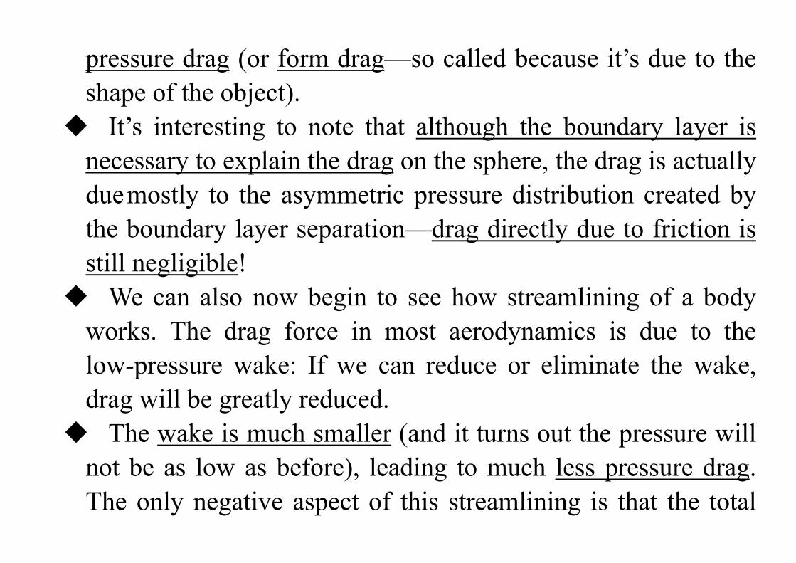
pressure drag (or form drag—so called because it’s due to the shape of the object). It’s interesting to note that although the boundary layer is

necessary to explain the drag on the sphere, the drag is actually due mostly to the asymmetric pressure distribution created by the boundary layer separation—drag directly due to friction is still negligible! We can also now begin to see how streamlining of a body

works. The drag force in most aerodynamics is due to the low-pressure wake: If we can reduce or eliminate the wake, drag will be greatly reduced. The wake is much smaller (and it turns out the pressure will

not be as low as before), leading to much less pressure drag. The only negative aspect of this streamlining is that the total

surface area on which friction occurs is larger, so drag due to friction will increase a little.

Laminar and Turbulent Flows If you turn on a faucet (that doesn’t have an aerator or other

attachment) at a very low flow rate the water will flow out

very smoothly—almost “glass-like.” If you increase the flow rate, the water will exit in a churned-up, chaotic manner. These are examples of how a viscous flow can be laminar or turbulent, respectively. A laminar flow is one in which the fluid particles move in

smooth layers, or laminas; a turbulent flow is one in which the fluid particles rapidly mix as they move along due to random three dimensional velocity fluctuations. Typical examples of pathlines of each of these are illustrated

in the following figure, which shows a one-dimensional flow.

In most fluid mechanics problems—for example, flow of water in a pipe—turbulence is an unwanted but often unavoidable phenomenon, because it generates more resistance to flow The flow of blood through blood vessels—it is desirable

because the random mixing allows all of the blood cells to contact the walls of the blood vessels to exchange oxygen and other nutrients. The velocity of the laminar flow is simply u; the velocity of

the turbulent flow is given by the mean velocity u plus the three components of randomly fluctuating velocity u’, v’, and w’. Although many turbulent flows of interest are steady in the

mean (u is not a function of time), the presence of the

random, high-frequency velocity fluctuations makes the analysis of turbulent flows extremely difficult. In a one-dimensional laminar flow, the shear stress is related to the velocity gradient by the simple relation

yxdudy

For a turbulent flow in which the mean velocity field is one-dimensional, no such simple relation is valid.

Random, three-dimensional velocity fluctuations (u’, v’, and w’) transport momentum across the mean flow streamlines, increasing the effective shear stress.

Consequently, in turbulent flow there is no universal relationship between the stress field and the mean-velocity field. Thus in turbulent flows we must rely heavily on

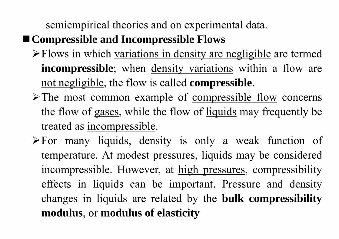
semiempirical theories and on experimental data. Compressible and Incompressible Flows Flows in which variations in density are negligible are termed

incompressible; when density variations within a flow are not negligible, the flow is called compressible. The most common example of compressible flow concerns

the flow of gases, while the flow of liquids may frequently be treated as incompressible. For many liquids, density is only a weak function of

temperature. At modest pressures, liquids may be considered incompressible. However, at high pressures, compressibility effects in liquids can be important. Pressure and density changes in liquids are related by the bulk compressibility modulus, or modulus of elasticity

/vdpE

d

If the bulk modulus is independent of temperature, then density is only a function of pressure (the fluid is barotropic). Bulk modulus data for some common liquids are given in Appendix A. Water hammer and cavitation are examples of the

importance of compressibility effects in liquid flows. Water hammer is caused by acoustic waves propagating and

reflecting in a confined liquid, for example, when a valve is closed abruptly. The resulting noise can be similar to “hammering” on the pipes, hence the term. Cavitation occurs when vapor pockets form in a liquid flow

because of local reductions in pressure (for example at the tip of a boat’s propeller blades). Depending on the number and distribution of particles in the liquid to which very small pockets of undissolved gas or air may attach, the local pressure at the onset of cavitation may be at or below the vapor pressure of the liquid. These particles act as nucleation sites to initiate vaporization. Vapor pressure of a liquid is the partial pressure of the vapor

in contact with the saturated liquid at a given temperature. When pressure in a liquid is reduced to less than the vapor pressure, the liquid may change phase suddenly and “flash” to vapor. The vapor pockets in a liquid flow may alter the geometry of

the flow field substantially. When adjacent to a surface, the

growth and collapse of vapor bubbles can cause serious damage by eroding the surface material. It turns out that gas flows with negligible heat transfer also

may be considered incompressible provided that the flow speeds are small relative to the speed of sound; the ratio of the flow speed, V, to the local speed of sound, c, in the gas is defined as the Mach number,

VMc

For M < 0.3, the maximum density variation is less than 5 percent. Thus gas flows with M < 0.3 can be treated as incompressible; a value of M = 0.3 in air at standard conditions corresponds to a speed of approximately 100 m/s. Compressible flows occur frequently in engineering

applications. Common examples include compressed air systems used to

power shop tools and dental drills, transmission of gases in pipelines at high pressure, and pneumatic or fluidic control and sensing systems. Compressibility effects are very important in the design of modern high-speed aircraft and missiles, power plants, fans, and compressors.

Internal and External Flows Flows completely bounded by solid surfaces are called

internal or duct flows. Flows over bodies immersed in an unbounded fluid are termed external flows. Both internal and external flows may be laminar or turbulent,

compressible or incompressible. We mentioned an example of internal flow when we

discussed the flow out of a faucet—the flow in the pipe leading to the faucet is an internal flow. It turns out that we have a Reynolds number for pipe flows defined as

/Re VD , where V is the average flow velocity and D is the pipe diameter (note that we do not use the pipe length!). This Reynolds number indicates whether a pipe flow will be laminar or turbulent. Flow will generally be laminar for Re 2300 and turbulent for larger values: Flow in a pipe of constant diameter will be entirely laminar or entirely turbulent, depending on the value of the velocity V. We already saw some examples of external flows when we

discussed the flow over a sphere and a streamlined object. What we didn’t mention was that these flows could be laminar or turbulent. In addition, we mentioned boundary

layers: It turns out these also can be laminar or turbulent. When we discuss these in detail (Chapter 9), we’ll start with the simplest kind of boundary layer—that over a flat plate—and learn that just as we have a Reynolds number for the overall external flow that indicates the relative significance of viscous forces, there will also be a boundary-layer Reynolds number /xRe U x where in

this case the characteristic velocity U is the velocity

immediately outside the boundary layer and the characteristic length x is the distance along the plate. Hence, at the leading edge of the plate 0xRe , and at the end of a plate of length L,

it will be Re /x U L .

The significance of this Reynolds number is that the boundary layer will be laminar for 55 10xRe and

turbulent for larger values: A boundary layer will start out laminar, and if the plate is long enough the boundary layer will transition to become turbulent. Both internal and external flows can be compressible or

incompressible. Compressible flows can be divided into subsonic and supersonic regimes. We will study compressible flows in Chapters 12 and 13 and

see among other things that supersonic flows (M>1) will behave very differently than subsonic flows (M<1). For example, supersonic flows can experience oblique and

normal shocks, and can also behave in a counterintuitive

way—e.g., a supersonic nozzle (a device to accelerate a flow) must be divergent (i.e., it has increasing cross-sectional area) in the direction of flow! We note here also that in a subsonic nozzle (which has a convergent cross-sectional area), the pressure of the flow at the exit plane will always be the ambient pressure; for a sonic flow, the exit pressure can be higher than ambient; and for a supersonic flow the exit pressure can be greater than, equal to, or less than the ambient pressure!

2.7 Summary and Useful Equations In this chapter we have completed our review of some of the

fundamental concepts we will utilize in our study of fluid mechanics. Some of these are:

How to describe flows (timelines, pathlines, streamlines, streaklines). Forces (surface, body) and stresses (shear, normal). Types of fluids (Newtonian, non-Newtonian—dilatant,

pseudoplastic, thixotropic, rheopectic, Bingham plastic) and viscosity (kinematic, dynamic, apparent). Types of flow (viscous/inviscid, laminar/turbulent,

compressible/incompressible, internal/external). We also briefly discussed some interesting phenomena, such

as surface tension, boundary layers, wakes, and streamlining. Finally, we introduced two very useful dimensionless groups—the Reynolds number and the Mach number.