Chapter 2: Everything you never wanted to know about ... › system › files › chapter2_1.pdf · DISCOVERINGSTATISTICS+USING+SPSS+ PROFESSOR’ANDY’PFIELD’ ’ 1’ Chapter

DISCOVERING STATISTICS USING SPSS

PROFESSOR ANDY P FIELD 1

Chapter 2: Everything you never wanted to know about statistics

Smart Alex’s Solutions

Task 1

Why do we use samples?

We are usually interested in populations, but because we cannot collect data from every human being (or whatever) in the population, we collect data from a small subset of the population (known as a sample) and use these data to infer things about the population as a whole.

Task 2

What is the mean and how do we tell if it’s representative of our data?

The mean is a simple statistical model of the centre of a distribution of scores. A hypothetical estimate of the ‘typical’ score. We use the variance, or standard deviation, to tell us whether it is representative of our data. The standard deviation is a measure of how much error there is associated with the mean: a small standard deviation indicates that the mean is a good representation of our data.

Task 3

What’s the difference between the standard deviation and the standard error?

The standard deviation tells us how much observations in our sample differ from the mean value within our sample. The standard error tells us not about how the sample mean represents the sample itself, but how well the sample mean represents the population mean. The standard error is the standard deviation of the sampling distribution of a statistic. For a given statistic (e.g. the mean) it tells us how much variability there is in this statistic across samples from the same population. Large values, therefore, indicate that a statistic from a given sample may not be an accurate reflection of the population from which the sample came.

Task 4

In Chapter 1 we used an example of the time in seconds taken for 21 heavy smokers to fall off a treadmill at the fastest setting (18, 16, 18, 24, 23, 22, 22, 23, 26, 29, 32, 34, 34, 36, 36, 43, 42, 49, 46, 46, 57). Calculate standard error and 95% confidence interval for these data.



If you did the tasks in Chapter 1, you’ll know that the mean is 32.19 seconds:

𝑋 =𝑥!!

!!!

𝑛

= 16 + 2 18 + 2 22 + 2 23 + 24 + 26 + 29 + 32 + 2 34 + 2 36 + 42 + 43 + 2 46 + 49 + 57

21

=67621

= 32.19

We also worked out that the sum of squared errors was 2685.24; the variance was 2685.24/20 =

134.26; the standard deviation is the square root of the variance, so was 134.26 = 11.59.

The standard error will be:

𝑆𝐸 =𝑠𝑁=11.5921

= 2.53

The sample is small, so to calculate the confidence interval we need to find the appropriate value of t. First we need to calculate the degrees of freedom, N − 1. With 21 data points, the degrees of freedom are 20. For a 95% confidence interval we can look up the value in the column labelled ‘Two-‐Tailed Test’, ‘.05’ in the table of critical values of the t-‐distribution (Appendix). The corresponding value is 2.09. The confidence intervals is, therefore, given by:

lower boundary of confidence interval = 𝑋 − 2.09×𝑆𝐸 = 32.19 – (2.09 × 2.53) = 26.90

upper boundary of confidence interval = 𝑋 + 2.09×𝑆𝐸 = 32.19 + (2.09 × 2.53) = 37.48

Task 5

What do the sum of squares, variance and standard deviation represent? How do they differ?

All of these measures tell us something about how well the mean fits the observed sample data. Large values (relative to the scale of measurement) suggest the mean is a poor fit of the observed scores, and small values suggest a good fit. They are also, therefore, measures of dispersion, with large values indicating a spread-‐out distribution of scores and small values showing a more tightly packed distribution. These measures all represent the same thing, but differ in how they express it. The sum of squared errors is a ‘total’ and is, therefore, affected by the number of data points. The variance is the ‘average’ variability but in units squared. The standard deviation is the average variation but converted back to the original units of measurement. As such, the size of the standard deviation can be compared to the mean (because they are in the same units of measurement).

Task 6

What is a test statistic and what does it tell us?

A test statistic is a statistic for which we know how frequently different values occur. The observed value of such a statistic is typically used to test hypotheses, or to establish whether a model is a reasonable representation of what’s happening in the population.



Task 7

What are Type I and Type II errors?

A Type I error occurs when we believe that there is a genuine effect in our population, when in fact there isn’t. A Type II error occurs when we believe that there is no effect in the population when, in reality, there is.

Task 8

What is an effect size and how is it measured?

An effect size is an objective and standardized measure of the magnitude of an observed effect. Measures include Cohen’s d, the odds ratio and Pearson’s correlations coefficient, r. Cohen’s d, for example, is the difference between two means divided by either the standard deviation of the control group, or by a pooled standard deviation.

Task 9

What is statistical power?

Power is the ability of a test to detect an effect of a particular size (a value of 0.8 is a good level to aim for).

Task 10

Figure 2.16 shows two experiments that looked at the effect of singing versus conversation on how much time a woman would spend with a man. In both experiments the means were 10 (singing) and 12 (conversation), the standard deviations in all groups were 3, but the group sizes were 10 per group in the first experiment and 100 per group in the second. Compute the values of the confidence intervals displayed in the Figure.

Experiment 1:

In both groups, because they have a standard deviation of 3 and a sample size of 10, the standard error will be:

𝑆𝐸 =𝑠𝑁=

310

= 0.95

The sample is small, so to calculate the confidence interval we need to find the appropriate value of t. First we need to calculate the degrees of freedom, N − 1. With 10 data points, the degrees of freedom are 9. For a 95% confidence interval we can look up the value in the column labelled ‘Two-‐Tailed Test’, ‘.05’ in the table of critical values of the t-‐distribution (Appendix). The corresponding value is 2.26. The confidence interval for the singing group is, therefore, given by:

lower boundary of confidence interval = 𝑋 − 2.26×𝑆𝐸 = 10 – (2.26 × 0.95) = 7.85

upper boundary of confidence interval = 𝑋 + 2.26×𝑆𝐸 = 10 + (2.26 × 0.95) = 12.15

For the conversation group:





Experiment 2:

In both groups, because they have a standard deviation of 3 and a sample size of 100, the standard error will be:

𝑆𝐸 =𝑠𝑁=

3100

= 0.33

The sample is large, so to calculate the confidence interval we need to find the appropriate value of z. For a 95% confidence interval we should look up the value of .025 in the column labelled Smaller Portion in the table of the standard normal distribution (Appendix). The corresponding value is 1.96. The confidence interval for the singing group is, therefore, given by:






Task 11

Figure 2.17 shows a similar study to above, but the means were 10 (singing) and 10.01 (conversation), the standard deviations in both groups were 3, and each group contained 1 million people. Compute the values of the confidence intervals displayed in the figure.

In both groups, because they have a standard deviation of 3 and a sample size of 1,000,000, the standard error will be:

𝑆𝐸 =𝑠𝑁=

31000000

= 0.003

The sample is large, so to calculate the confidence interval we need to find the appropriate value of z. For a 95% confidence interval we should look up the value of .025 in the column labelled Smaller Portion in the table of the standard normal distribution (Appendix). The corresponding value is 1.96. The confidence interval for the singing group is, therefore, given by:






Note: these values will look slightly different than the graph because the exact means were 10.00147 and 10.01006, but we rounded off to 10 and 10.01 to make life a bit easier. If you use these exact values you’d get, for the singing group:

lower boundary of confidence interval = 10.00147 – (1.96 × 0.003) = 9.99559

upper boundary of confidence interval = 10.00147 + (1.96 × 0.003) = 10.00735




lower boundary of confidence interval = 10.01006 – (1.96 × 0.003) = 10.00418

upper boundary of confidence interval = 10.01006 + (1.96 × 0.003) = 10.01594

Task 12

In Chapter 1 (Task 8) we looked at an example of how many games it took a sportsperson before they hit the ‘red zone’ Calculate the standard error and confidence interval for those data.

We worked out in Chapter 1 that the mean was 10.27, the standard deviation 4.15, and there were 11 sportspeople in the sample. The standard error will be:

𝑆𝐸 =𝑠𝑁=4.1511

= 1.25

The sample is small, so to calculate the confidence interval we need to find the appropriate value of t. First we need to calculate the degrees of freedom, N − 1. With 11 data points, the degrees of freedom are 10. For a 95% confidence interval we can look up the value in the column labelled ‘Two-‐Tailed Test’, ‘.05’ in the table of critical values of the t-‐distribution (Appendix). The corresponding value is 2.23. The confidence interval is, therefore, given by:



Task 13

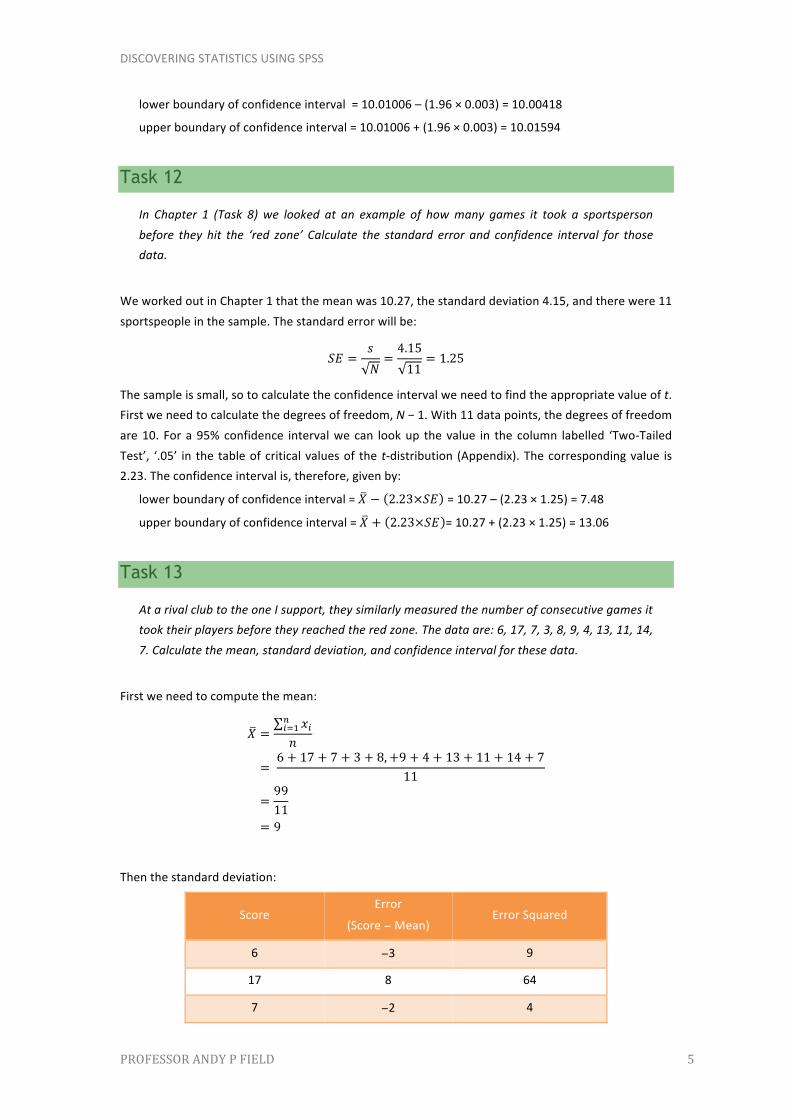
At a rival club to the one I support, they similarly measured the number of consecutive games it took their players before they reached the red zone. The data are: 6, 17, 7, 3, 8, 9, 4, 13, 11, 14, 7. Calculate the mean, standard deviation, and confidence interval for these data.

First we need to compute the mean:

𝑋 =𝑥!!

!!!

𝑛

= 6 + 17 + 7 + 3 + 8,+9 + 4 + 13 + 11 + 14 + 7

11

=9911

= 9

Then the standard deviation:

Score Error

(Score − Mean) Error Squared

6 −3 9

17 8 64

7 −2 4



3 −6 36

8 −1 1

9 0 0

4 −5 25

13 4 16

11 2 4

14 5 25

7 −2 4

Sum of squared error = 9 + 64 + 4 + 36 + 1 + 0 + 25 + 16 + 4 + 25 + 4 = 188.

Variance:

𝑠! =sum of squares

𝑛 − 1=18810

= 18.8

Standard deviation:

𝑠 = variance = 18.8 = 4.34

There were 11 sportspeople in the sample, so the standard error will be:

𝑆𝐸 =𝑠𝑁=4.3411

= 1.31

The sample is small, so to calculate the confidence interval we need to find the appropriate value of t. First we need to calculate the degrees of freedom, N − 1. With 11 data points, the degrees of freedom are 10. For a 95% confidence interval we can look up the value in the column labelled ‘Two-‐Tailed Test’, ‘.05’ in the table of critical values of the t-‐distribution (Appendix). The corresponding value is 2.23. The confidence intervals is, therefore, given by:



Task 14

Compute and interpret Cohen’s d for the difference in the mean number of games it took players to become fatigued in the two teams mentioned in the previous two tasks.

Cohen’s d is defined as:

1 2ˆ X Xds−

=

There isn’t an obvious control group, so let's use a pooled estimate of the standard deviation:

𝑠! =𝑁! − 1 𝑠!! + 𝑁! − 1 𝑠!!

𝑁! + 𝑁! − 2=

11 − 1 4.15! + 11 − 1 4.34!

11 + 11 − 2=

360.2320

= 4.24



Therefore, Cohen’s d is:

10.27 9ˆ .304.24

d −= =

Therefore, the second team fatigued in fewer matches than the first team by about 1/3 standard deviation. By the benchmarks that we probably shouldn’t use, this is a small to medium effect, but I guess if you’re managing a top-‐flight sports team, fatiguing 1/3 of a standard deviation faster than one of your opponents could make quite a substantial difference to your performance and team rotation over the season.

Task 15

In Chapter 1 (Task 9) we looked at the length in days of nine celebrity marriages. Here are the length in days of eight marriages, one being mine and the other seven being those of some of my friends and family (in all but one case up to the day I’m writing this, which is 8 March 2012, but in the 91-‐day case it was the entire duration – this isn’t my marriage, in case you’re wondering: 210, 91, 3901, 1339, 662, 453, 16672, 21963, 222. Calculate the mean, standard deviation and confidence interval for these data.

First we need to compute the mean:

𝑋 =𝑥!!

!!!

𝑛

= 210 + 91 + 3901 + 1339 + 662 + 453 + 16672 + 21963 + 222

9

=455139

= 5057

Then the standard deviation:

Score Error

(Score − Mean) Error Squared

210 −4847 23493409

91 −4966 24661156

3901 −1156 1336336

1339 −3718 13823524

662 −4395 19316025

453 −4604 21196816

16672 11615 134908225

21963 16906 285812836

222 −4835 23377225



Sum of squared error = 23493409 + 24661156 + 1336336 + 13823524 + 19316025 + 21196816 + 134908225 + 285812836 + 23377225 = 547925552

Variance:

𝑠! =sum of squares

𝑛 − 1=547925552

8= 68490694

Standard deviation:

𝑠 = variance = 68490694 = 8275.91

The standard error will be:

𝑆𝐸 =𝑠𝑁=8275.91

9= 2758.64

The sample is small, so to calculate the confidence interval we need to find the appropriate value of t. First we need to calculate the degrees of freedom, N − 1. With 9 data points, the degrees of freedom are 8. For a 95% confidence interval we can look up the value in the column labelled ‘Two-‐Tailed Test’, ‘.05’ in the table of critical values of the t-‐distribution (Appendix). The corresponding value is 2.31. The confidence interval is, therefore, given by:

lower boundary of CI = 𝑋 − 2.31×𝑆𝐸 = 5057 – (2.31 × 2758.64) = −1315.46

upper boundary of CI = 𝑋 + 2.31×𝑆𝐸 = 5057 + (2.31× 2758.64) = 11429.46

Task 16

Calculate and interpret Cohen’s d for the difference in the mean duration of the celebrity marriages in Chapter 1 and me and my friend’s marriages.

Cohen’s d is defined as:

1 2ˆ X Xds−

=

There isn’t an obvious control group, so let's use a pooled estimate of the standard deviation:

𝑠! =𝑁! − 1 𝑠!! + 𝑁! − 1 𝑠!!

𝑁! + 𝑁! − 2=

11 − 1 476.29! + 9 − 1 8275.91!

11 + 9 − 2

=550194093

18

= 5528.68

Therefore, Cohen’s d is:

𝑑 =5057 − 238.91

5528.68= 0.87

Therefore, my friend’s marriages are 0.87 standard deviations longer than the sample of celebrities. By the benchmarks that we probably shouldn’t use, this is a large effect.



Task 17

What are the problems with null hypothesis significance testing?

1. We can’t conclude that an effect is important because the p-‐value from which we determine significance is affected by sample size. Therefore, the word ‘significant’ is meaningless when referring to a p-‐value.

2. The null hypothesis is never true. If the p-‐value is greater than .05 then we can decide to reject the alternative hypothesis, but this is not the same thing as the null hypothesis being true: a non-‐significant result tells us is that the effect is not big enough to be found but it doesn’t tell us that the effect is zero.

3. A significant result does not tell us that the null hypothesis is false (see text for details). 4. It encourages all or nothing thinking: if p <. 05 then an effect is significant, but if p > .05 it is

not. So, a p = .0499 is significant but a p = .0501 is not, even though these ps differ by only .0002.

Documents

Chapter 2: Everything you never wanted to know about ... › system › files › chapter2_1.pdf · DISCOVERINGSTATISTICS+USING+SPSS+ PROFESSOR’ANDY’PFIELD’ ’ 1’ Chapter