Chapter 2 Differentiation 2.3 Product and Quotient Rules

118 Chapter 2 Differentiation

2.3 Product and Quotient Rules and Higher-Order Derivatives

Find the derivative of a function using the Product Rule.Find the derivative of a function using the Quotient Rule.Find the derivative of a trigonometric function.Find a higher-order derivative of a function.

The Product RuleIn Section 2.2, you learned that the derivative of the sum of two functions is simply thesum of their derivatives. The rules for the derivatives of the product and quotient of twofunctions are not as simple.

Proof Some mathematical proofs, such as the proof of the Sum Rule, are straight-forward. Others involve clever steps that may appear unmotivated to a reader. Thisproof involves such a step—subtracting and adding the same quantity—which is shownin color.

Note that because is given to be differentiable and therefore

is continuous.See LarsonCalculus.com for Bruce Edwards’s video of this proof.

The Product Rule can be extended to cover products involving more than twofactors. For example, if and are differentiable functions of then

So, the derivative of is

� 2x sin x cos x � x2�cos2 x � sin2 x�.

dydx

� 2x sin x cos x � x2 cos x cos x � x2 sin x��sin x�

y � x2 sin x cos x

ddx

� f�x�g�x�h�x�� f��x�g�x�h�x� � f�x�g��x�h�x� � f�x�g�x�h��x�.

x,hg,f,

flim�x→0

f �x � �x� � f �x�

THEOREM 2.7 The Product Rule

The product of two differentiable functions and is itself differentiable.Moreover, the derivative of is the first function times the derivative of the second, plus the second function times the derivative of the first.

ddx

� f�x�g�x�� f�x�g��x� � g�x� f��x�

fggf

� f�x�g��x� � g�x�f��x�

� lim�x→0

f�x � �x� � lim�x→0

g�x � �x� � g�x��x

� lim�x→0

g�x� � lim�x→0

f�x � �x� � f�x��x

� lim�x→0 �f�x � �x�g�x � �x� � g�x�

�x � � lim�x→0 �g�x� f�x � �x� � f�x�

�x �

� lim�x→0 �f�x � �x�g�x � �x� � g�x�

�x� g�x� f�x � �x� � f�x�

� x �

� lim�x→0

f�x � �x�g�x � �x� � f�x � �x�g�x� � f�x � �x�g�x� � f�x�g�x��x

ddx

� f�x�g�x�� lim�x→0

f�x � �x�g�x � �x� � f�x�g�x�� x

REMARK A version of theProduct Rule that some peopleprefer is

The advantage of this form is that it generalizes easily to products of three or more factors.

REMARK The proof of theProduct Rule for products ofmore than two factors is left asan exercise (see Exercise 137).

ddx

� f�x�g�x�� f��x�g�x� � f�x�g��x�.

Copyright 2012 Cengage Learning. All Rights Reserved. May not be copied, scanned, or duplicated, in whole or in part. Due to electronic rights, some third party content may be suppressed from the eBook and/or eChapter(s). Editorial review has deemed that any suppressed content does not materially affect the overall learning experience. Cengage Learning reserves the right to remove additional content at any time if subsequent rights restrictions require it.

The derivative of a product of two functions is not (in general) given by the productof the derivatives of the two functions. To see this, try comparing the product of the derivatives of

and

with the derivative in Example 1.

Using the Product Rule

Find the derivative of

Solution

Apply Product Rule.

In Example 1, you have the option of finding the derivative with or without theProduct Rule. To find the derivative without the Product Rule, you can write

In the next example, you must use the Product Rule.



Solution

Apply Product Rule.



Solution

� �2x sin x

� �2x��sin x� � �cos x��2� � 2�cos x�

dydx

� �2x�� ddx

�cos x� � �cos x�� ddx

�2x� � 2 ddx

�sin x�

y � 2x cos x � 2 sin x.

� 3x�x cos x � 2 sin x� � 3x2 cos x � 6x sin x

� 3x2 cos x � �sin x��6x�

ddx

�3x2 sin x� � 3x2 ddx

�sin x� � sin x ddx

�3x2�

y � 3x2 sin x.

� �24x2 � 4x � 15.

Dx ��3x � 2x2��5 � 4x�� Dx��8x3 � 2x2 � 15x�

� �24x2 � 4x � 15

� �12x � 8x2� � �15 � 8x � 16x2� � �3x � 2x2��4� � �5 � 4x��3 � 4x�

h��x� � �3x � 2x2� ddx

�5 � 4x� � �5 � 4x� ddx

�3x � 2x2�

h�x� � �3x � 2x2��5 � 4x�.

g�x� � 5 � 4x

f�x� � 3x � 2x2

2.3 Product and Quotient Rules and Higher-Order Derivatives 119

FirstDerivative of

secondDerivative

of firstSecond

Product Rule Constant Multiple Rule

THE PRODUCT RULE

When Leibniz originally wrote aformula for the Product Rule, hewas motivated by the expression

from which he subtracted (as being negligible) and obtainedthe differential form This derivation resulted in the traditional form of the ProductRule. (Source: The History ofMathematics by David M. Burton)

x dy � y dx.

dx dy

�x � dx��y � dy� � xy

REMARK In Example 3,notice that you use the ProductRule when both factors of theproduct are variable, and youuse the Constant Multiple Rulewhen one of the factors is a constant.


The Quotient Rule

Proof As with the proof of Theorem 2.7, the key to this proof is subtracting andadding the same quantity.

Definition of derivative

Note that because is given to be differentiable and therefore

is continuous.See LarsonCalculus.com for Bruce Edwards’s video of this proof.

Using the Quotient Rule


Solution

Apply Quotient Rule.

��5x2 � 4x � 5

�x2 � 1�2

��5x2 � 5� � �10x2 � 4x�

�x2 � 1�2

��x2 � 1��5� � �5x � 2��2x�

�x2 � 1�2

ddx �

5x � 2x2 � 1� �

�x2 � 1� ddx

�5x � 2� � �5x � 2� ddx

�x2 � 1�

�x2 � 1�2

y �5x � 2x2 � 1

.

glim�x→0

g�x � �x� � g�x�

�g�x� f��x� � f�x�g��x�

�g�x��2

�g�x�� lim

�x→0 f�x � �x� � f�x�

�x � � f�x�� lim�x→0

g�x � �x� � g�x�

�x �lim

�x→0 �g�x�g�x � �x��

�lim

�x→0 g�x�� f�x � � x� � f�x��

�x� lim

�x→0 f�x��g�x � �x� � g�x��

�xlim

�x→0 �g�x�g�x � �x��

� lim�x→0

g�x�f�x � �x� � f�x�g�x� � f�x�g�x� � f�x�g�x � �x�

�xg�x�g�x � �x�

� lim�x→0

g�x� f�x � �x� � f�x�g�x � �x�

�xg�x�g�x � �x�

d

dx�f�x�g�x�� lim

�x→0

f�x � �x�g�x � �x� �

f�x�g�x�

�x


y ′ = −5x2 + 4x + 5(x2 + 1)2

−4

−7 8

6

y = 5x − 2x2 + 1

Graphical comparison of a function and its derivativeFigure 2.22

THEOREM 2.8 The Quotient Rule

The quotient of two differentiable functions and is itself differentiable at all values of for which Moreover, the derivative of is given by the denominator times the derivative of the numerator minus the numeratortimes the derivative of the denominator, all divided by the square of thedenominator.

g�x� � 0d

dx�f�x�g�x��

g�x� f��x� � f�x�g��x��g�x��2 ,

fgg�x� � 0.xgffg

REMARK From the QuotientRule, you can see that the derivative of a quotient is not (in general) the quotient of the derivatives.

TECHNOLOGY A graphingutility can be used to comparethe graph of a function with the graph of its derivative. For instance, in Figure 2.22,the graph of the function inExample 4 appears to have two points that have horizontal tangent lines. What are the values of at these two points?y�


Note the use of parentheses in Example 4. A liberal use of parentheses is recommended for all types of differentiation problems. For instance, with the QuotientRule, it is a good idea to enclose all factors and derivatives in parentheses, and to payspecial attention to the subtraction required in the numerator.

When differentiation rules were introduced in the preceding section, the need forrewriting before differentiating was emphasized. The next example illustrates this pointwith the Quotient Rule.

Rewriting Before Differentiating

Find an equation of the tangent line to the graph of at

Solution Begin by rewriting the function.

Write original function.

Multiply numerator and denominator by

Rewrite.

Next, apply the Quotient Rule.

Quotient Rule

Simplify.

To find the slope at evaluate

Slope of graph at

Then, using the point-slope form of the equation of a line, you can determine that theequation of the tangent line at is See Figure 2.23.

Not every quotient needs to be differentiated by the Quotient Rule. For instance,each quotient in the next example can be considered as the product of a constant timesa function of In such cases, it is more convenient to use the Constant Multiple Rule.

Using the Constant Multiple Rule

Original Function Rewrite Differentiate Simplify

a.

b.

c.

d. y� � �185x3y� �

95

��2x�3�y �95

�x�2�y �9

5x2

y� �67

y� � �37

��2�y � �37

�3 � 2x�y ��3�3x � 2x2�

7x

y� �52

x3y� �58

�4x3�y �58

x4y �5x4

8

y� �2x � 3

6y� �

16

�2x � 3�y �16

�x2 � 3x�y �x2 � 3x

6

x.

y � 1.��1, 1�

��1, 1�f ��1� � 0

f��1�.��1, 1�,

��3x2 � 2x � 5

�x2 � 5x�2

��3x2 � 15x� � �6x2 � 13x � 5�

�x2 � 5x�2

f � �x� ��x2 � 5x��3� � �3x � 1��2x � 5�

�x2 � 5x�2

�3x � 1x2 � 5x

x. �x�3 �

1x

x�x � 5�

f �x� �3 � �1x�

x � 5

��1, 1�.f �x� �3 � �1x�

x � 5


y

x

y = 1

f (x) = 3 − 1

x + 5x

−1−2−3−4−5−6−7 1 2 3

−2

−3

−4

−5

3

4

5

(−1, 1)

The line is tangent to the graphof at the point Figure 2.23

��1, 1�.f �x�y � 1

REMARK To see the benefitof using the Constant MultipleRule for some quotients, tryusing the Quotient Rule to differentiate the functions inExample 6—you should obtain the same results, but with more work.


In Section 2.2, the Power Rule was proved only for the case in which the exponent is a positive integer greater than 1. The next example extends the proof toinclude negative integer exponents.

Power Rule: Negative Integer Exponents

If is a negative integer, then there exists a positive integer such that So, bythe Quotient Rule, you can write

Quotient Rule and Power Rule

So, the Power Rule

Power Rule

is valid for any integer. In Exercise 71 in Section 2.5, you are asked to prove the casefor which is any rational number.

Derivatives of Trigonometric FunctionsKnowing the derivatives of the sine and cosine functions, you can use the Quotient Ruleto find the derivatives of the four remaining trigonometric functions.

Proof Considering and applying the Quotient Rule, youobtain

Apply Quotient Rule.

See LarsonCalculus.com for Bruce Edwards’s video of this proof.

The proofs of the other three parts of the theorem are left as an exercise (see Exercise 87).

� sec2 x.

�1

cos2 x

�cos2 x � sin2 x

cos2 x

��cos x��cos x� � �sin x��sin x�

cos2 x

ddx

�tan x� �ddx�

sin xcos x�

tan x � �sin x��cos x�

n

ddx

�xn� � nxn�1

n � �k � nxn�1.

� �kx�k�1

�0 � kxk�1

x2k

�xk�0� � �1��kxk�1�

�xk�2

d

dx�xn� �

ddx�

1xk�

n � �k.kn

n


THEOREM 2.9 Derivatives of Trigonometric Functions

ddx

�csc x� � �csc x cot xddx

�sec x� � sec x tan x

ddx

�cot x� � �csc2 xddx

�tan x� � sec2 x

REMARK In the proof ofTheorem 2.9, note the use of the trigonometric identities

and

These trigonometric identitiesand others are listed inAppendix C and on the formula cards for this text.

sec x �1

cos x.

sin2 x � cos2 x � 1


Differentiating Trigonometric Functions

See LarsonCalculus.com for an interactive version of this type of example.

Function Derivative

a.

b.

Different Forms of a Derivative

Differentiate both forms of

Solution

First form:

Second form:

To show that the two derivatives are equal, you can write

The summary below shows that much of the work in obtaining a simplified formof a derivative occurs after differentiating. Note that two characteristics of a simplifiedform are the absence of negative exponents and the combining of like terms.

� csc2 x � csc x cot x.

�1

sin2 x� � 1

sin x�cos xsin x

1 � cos x

sin2 x�

1sin2 x

�cos xsin2 x

y� � �csc x cot x � csc2 x

y � csc x � cot x

sin2 x � cos2 x � 1 �1 � cos x

sin2 x

�sin2 x � cos x � cos2 x

sin2 x

y� ��sin x��sin x� � �1 � cos x��cos x�

sin2 x

y �1 � cos x

sin x

y �1 � cos x

sin x� csc x � cot x.

� �sec x��1 � x tan x� y� � x�sec x tan x� � �sec x��1�y � x sec x

dydx

� 1 � sec2 xy � x � tan x


REMARK Because oftrigonometric identities, thederivative of a trigonometricfunction can take many forms.This presents a challenge whenyou are trying to match youranswers to those given in theback of the text.

After Differentiatingf��x� After Simplifyingf��x�

Example 1 �3x � 2x2��4� � �5 � 4x��3 � 4x� �24x2 � 4x � 15

Example 3 �2x��sin x� � �cos x��2� � 2�cos x� �2x sin x

Example 4�x2 � 1��5� � �5x � 2��2x�

�x2 � 1�2

�5x2 � 4x � 5�x2 � 1�2

Example 5�x2 � 5x��3� � �3x � 1��2x � 5�

�x2 � 5x�2

�3x2 � 2x � 5�x2 � 5x�2

Example 6�sin x��sin x� � �1 � cos x��cos x�

sin2 x1 � cos x

sin2 x


Higher-Order DerivativesJust as you can obtain a velocity function by differentiating a position function, you can obtain an acceleration function by differentiating a velocity function. Another wayof looking at this is that you can obtain an acceleration function by differentiating aposition function twice.

Position function

Velocity function

Acceleration function

The function is the second derivative of and is denoted by The second derivative is an example of a higher-order derivative. You can define

derivatives of any positive integer order. For instance, the third derivative is the deriv-ative of the second derivative. Higher-order derivatives are denoted as shown below.

First derivative:

Second derivative:

Third derivative:

Fourth derivative:

nth derivative:

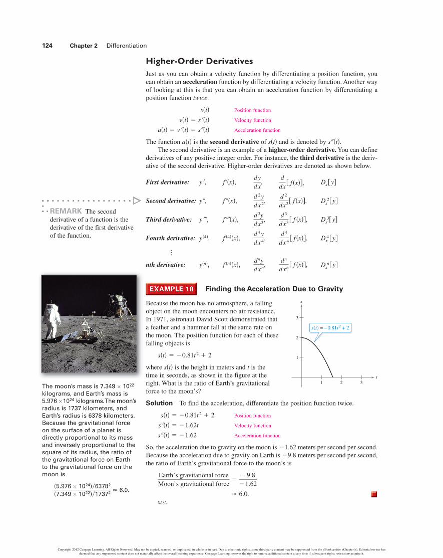
Finding the Acceleration Due to Gravity

Because the moon has no atmosphere, a fallingobject on the moon encounters no air resistance. In 1971, astronaut David Scott demonstrated that a feather and a hammer fall at the same rate on the moon. The position function for each of thesefalling objects is

where is the height in meters and is the time in seconds, as shown in the figure at the right. What is the ratio of Earth’s gravitationalforce to the moon’s?

Solution To find the acceleration, differentiate the position function twice.

Position function

Velocity function

Acceleration function

So, the acceleration due to gravity on the moon is meters per second per second.Because the acceleration due to gravity on Earth is meters per second per second,the ratio of Earth’s gravitational force to the moon’s is

� 6.0.

Earth’s gravitational forceMoon’s gravitational force

��9.8�1.62

�9.8�1.62

s �t� � �1.62

s��t� � �1.62t

s�t� � �0.81t2 � 2

ts�t�

s�t� � �0.81t2 � 2

Dxn�y�dn

dxn � f �x��,dnydxn,f �n��x�,y�n�,

�

Dx4 �y�d4

dx4 � f�x��,d4ydx4,f �4��x�,y�4�,

Dx3�y�d3

dx3 � f �x��,d3ydx3,f��x�,y��,

Dx2�y�d 2

dx2 � f�x��,d 2ydx2,f �x�,y,

Dx �y�ddx

� f�x��,dydx

,f��x�,y�,

s �t�.s�t�a�t�

a�t� � v��t� � s�t� v�t� � s��t�

s�t�


The moon’s mass is kilograms, and Earth’s mass is

kilograms.The moon’sradius is 1737 kilometers, andEarth’s radius is 6378 kilometers.Because the gravitational forceon the surface of a planet isdirectly proportional to its massand inversely proportional to thesquare of its radius, the ratio ofthe gravitational force on Earth to the gravitational force on themoon is

�5.976 1024�63782

�7.349 1022�17372 � 6.0.

5.976 1024

7.349 1022

REMARK The second derivative of a function is the derivative of the first derivativeof the function.

1 2 3

1

2

3

t

s

s(t) = −0.81t2 + 2

NASA



Using the Product Rule In Exercises 1–6, use the ProductRule to find the derivative of the function.

1. 2.

3. 4.

5. 6.

Using the Quotient Rule In Exercises 7–12, use theQuotient Rule to find the derivative of the function.

7. 8.

9. 10.

11. 12.

Finding and Evaluating a Derivative In Exercises 13–18,find and

Function Value of c

13.

14.

15.

16.

17.

18.

Using the Constant Multiple Rule In Exercises 19–24,complete the table to find the derivative of the function withoutusing the Quotient Rule.

Function Rewrite Differentiate Simplify

19.

20.

21.

22.

23.

24.

Finding a Derivative In Exercises 25–38, find the derivativeof the algebraic function.

25. 26.

27. 28.

29. 30.

31. 32.

33.

34.

35.

36.

37. is a constant

38. is a constant

Finding a Derivative of a Trigonometric Function InExercises 39–54, find the derivative of the trigonometric function.

39. 40.

41. 42.

43. 44.

45. 46.

47. 48.

49. 50.

51. 52.

53. 54.

Finding a Derivative Using Technology In Exercises55–58, use a computer algebra system to find the derivative ofthe function.

55.

56.

57.

58. f �� sin �

1 � cos �

g��

1 � sin �

f �x� � �x2 � x � 3x2 � 1 �x2 � x � 1�

g�x� � �x � 1x � 2�2x � 5�

h�� 5� sec � � � tan �y � 2x sin x � x2 cos x

f �x� � sin x cos xf �x� � x 2 tan x

y � x sin x � cos xy � �csc x � sin x

y �sec x

xy �

3�1 � sin x�2 cos x

h�x� �1x

� 12 sec xg�t� � 4�t � 6 csc t

y � x � cot xf �x� � �x � tan x

f �x� �sin x

x3f �t� �cos t

t

f �� 1� cos �f �t� � t 2 sin t

cf �x� �c2 � x 2

c2 � x 2,

cf �x� �x2 � c2

x2 � c2,

f �x� � �x3 � x��x2 � 2��x2 � x � 1�f �x� � �2x3 � 5x��x � 3��x � 2�

g�x� � x2�2x

�1

x � 1

f �x� �

2 �1x

x � 3

h�x� � �x2 � 3�3h�s� � �s3 � 2�2

f �x� � 3�x��x � 3�f �x� �3x � 1�x

f �x� � x 4�1 �2

x � 1f �x� � x�1 �4

x � 3

f �x� �x2 � 5x � 6

x2 � 4f �x� �

4 � 3x � x 2

x 2 � 1

y �2xx13

y �4x32

x

y �103x3

y �6

7x2

y �5x2 � 3

4

y �x2 � 3x

7

c ��

6f �x� �

sin xx

c ��

4f �x� � x cos x

c � 3f �x� �x � 4x � 4

c � 1f �x� �x2 � 4x � 3

c � 2y � �x2 � 3x � 2��x3 � 1�c � 0f �x� � �x3 � 4x��3x 2 � 2x � 5�

f� c�.f� x�

f �t� �cos t

t3g�x� �sin x

x2

f �x� �x2

2�x � 1h�x� �

�xx3 � 1

g�t� �3t2 � 12t � 5

f �x� �x

x2 � 1

g�x� � �x sin xf �x� � x3 cos x

g�s� � �s�s2 � 8�h�t� � �t�1 � t2�y � �3x � 4��x3 � 5�g�x� � �x2 � 3��x2 � 4x�

2.3 Exercises See CalcChat.com for tutorial help and worked-out solutions to odd-numbered exercises.



Evaluating a Derivative In Exercises 59–62, evaluate thederivative of the function at the given point. Use a graphingutility to verify your result.

Function Point

59.

60.

61.

62.

Finding an Equation of a Tangent Line In Exercises63–68, (a) find an equation of the tangent line to the graph of

at the given point, (b) use a graphing utility to graph thefunction and its tangent line at the point, and (c) use the derivative feature of a graphing utility to confirm your results.

63.

64.

65. 66.

67. 68.

Famous Curves In Exercises 69–72, find an equation of thetangent line to the graph at the given point. (The graphs inExercises 69 and 70 are called Witches of Agnesi. The graphs inExercises 71 and 72 are called serpentines.)

69. 70.

71. 72.

Horizontal Tangent Line In Exercises 73–76, determinethe point(s) at which the graph of the function has a horizontaltangent line.

73. 74.

75. 76.

77. Tangent Lines Find equations of the tangent lines to thegraph of that are parallel to the line

Then graph the function and the tangent lines.

78. Tangent Lines Find equations of the tangent lines to thegraph of that pass through the point Then graph the function and the tangent lines.

Exploring a Relationship In Exercises 79 and 80, verifythat and explain the relationship between and

79.

80.

Evaluating Derivatives In Exercises 81 and 82, use thegraphs of and Let and

81. (a) Find 82. (a) Find

(b) Find (b) Find

83. Area The length of a rectangle is given by and itsheight is where is time in seconds and the dimensions arein centimeters. Find the rate of change of the area with respectto time.

84. Volume The radius of a right circular cylinder is given byand its height is where is time in seconds and

the dimensions are in inches. Find the rate of change of thevolume with respect to time.

85. Inventory Replenishment The ordering and transporta-tion cost for the components used in manufacturing aproduct is

where is measured in thousands of dollars and is the ordersize in hundreds. Find the rate of change of with respect to

when (a) (b) and (c) What do theserates of change imply about increasing order size?

86. Population Growth A population of 500 bacteria isintroduced into a culture and grows in number according to theequation

where is measured in hours. Find the rate at which the population is growing when t � 2.

t

P�t� � 500�1 �4t

50 � t2

x � 20.x � 15,x � 10,xC

xC

x 1C � 100�200x2 �

xx � 30,

C

t12�t,�t � 2

t�t,6t � 5

y

x2−2 4 6 8 10

2

4

8

10

f

g

y

x

f

g

2−2 4 6 8 10

2

6

8

10

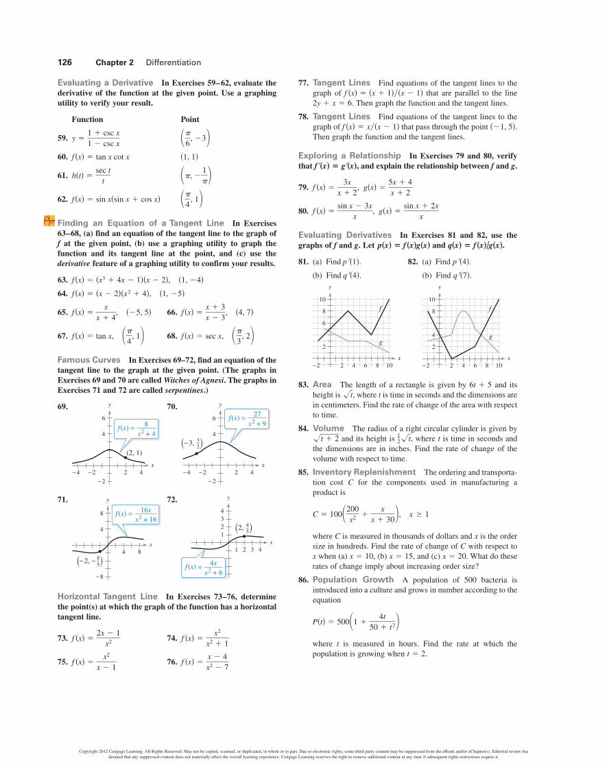
q��7�.q��4�.p��4�.p��1�.

q x� � f x�/g x�.p x� � f x�g x�g.f

g�x� �sin x � 2x

xf �x� �

sin x � 3xx

,

g�x� �5x � 4x � 2

f �x� �3x

x � 2,

g.ff� x� � g� x�,

��1, 5�.f �x� � x�x � 1�

2y � x � 6.f �x� � �x � 1��x � 1�

f �x� �x � 4x2 � 7

f �x� �x2

x � 1

f �x� �x2

x2 � 1f �x� �

2x � 1x2

y

x21 3 4

23

1

4

f (x) = 4xx2 + 6

2, 45( (

y

x4 8

−8

4

8 f (x) = 16xx2 + 16

−2, − 85( (

y

x2 4−2

−2

−4

4

6 f (x) = 27x2 + 9

−3, 32( (

y

x2 4−2

−2

−4

4

6

f (x) = 8x2 + 4

(2, 1)

��

3, 2f �x� � sec x,��

4, 1f �x� � tan x,

�4, 7�f �x� �x � 3x � 3

,��5, 5�f �x� �x

x � 4,

�1, �5�f �x� � �x � 2��x2 � 4�,�1, �4�f �x� � �x3 � 4x � 1��x � 2�,

f

��

4, 1f �x� � sin x�sin x � cos x�

��, �1�h�t� �

sec tt

�1, 1�f �x� � tan x cot x

��

6, �3y �

1 � csc x1 � csc x



87. Proof Prove the following differentiation rules.

(a)

(b)

(c)

88. Rate of Change Determine whether there exist any values of in the interval such that the rate of changeof and the rate of change of areequal.

89. Modeling Data The table shows the health care expenditures (in billions of dollars) in the United States andthe population (in millions) of the United States for the years2004 through 2009. The year is represented by with corresponding to 2004. (Source: U.S. Centers for Medicare& Medicaid Services and U.S. Census Bureau)

(a) Use a graphing utility to find linear models for the healthcare expenditures and the population

(b) Use a graphing utility to graph each model found in part(a).

(c) Find then graph using a graphing utility.What does this function represent?

(d) Find and interpret in the context of these data.

90. Satellites When satellites observe Earth, they can scanonly part of Earth’s surface. Some satellites have sensors thatcan measure the angle shown in the figure. Let representthe satellite’s distance from Earth’s surface, and let representEarth’s radius.

(a) Show that

(b) Find the rate at which is changing with respect to when(Assume miles.)

Finding a Second Derivative In Exercises 91–98, find thesecond derivative of the function.

91. 92.

93. 94.

95. 96.

97. 98.

Finding a Higher-Order Derivative In Exercises 99–102,find the given higher-order derivative.

99.

100.

101.

102.

Using Relationships In Exercises 103–106, use the giveninformation to find

and

and

103.

104.

105.

106.

Sketching Graphs In Exercises 111–114, the graph of isshown. Sketch the graphs of and To print an enlargedcopy of the graph, go to MathGraphs.com.

111. 112. y

x

f4

−4

−8

4

8

y

x

f

−2−4 4−2

2

4

f.f�f

f �x� � g�x�h�x�

f �x� �g�x�h�x�

f �x� � 4 � h�x�f �x� � 2g�x� � h�x�

h� 2� � 4h 2� � �1

g� 2� � �2g 2� � 3

f� 2�.

f �6��x�f �4��x� � 2x � 1,

f �4��x�f��x� � 2�x,

f��x�f �x� � 2 �2x,

f �x�f��x� � x 2,

f �x� � sec xf �x� � x sin x

f �x� �x2 � 3xx � 4

f �x� �x

x � 1

f �x� � x2 � 3x�3f �x� � 4x32

f �x� � 4x5 � 2x3 � 5x2f �x� � x4 � 2x3 � 3x2 � x

r � 3960� � 30�.�h

h � r �csc � � 1�.

r

r hθ

rh�

A��t�

AA � h�t�p�t�,

p�t�.h�t�

Year, t 4 5 6 7 8 9

h 1773 1890 2017 2135 2234 2330

p 293 296 299 302 305 307

t � 4t,p

h

g�x� � csc xf �x� � sec x�0, 2� �x

ddx

�cot x� � �csc2 x

ddx

�csc x� � �csc x cot x

ddx

�sec x� � sec x tan x

WRITING ABOUT CONCEPTS107. Sketching a Graph Sketch the graph of a differen-

tiable function such that forand for Explain how

you found your answer.

108. Sketching a Graph Sketch the graph of a differen-tiable function such that and for all realnumbers Explain how you found your answer.

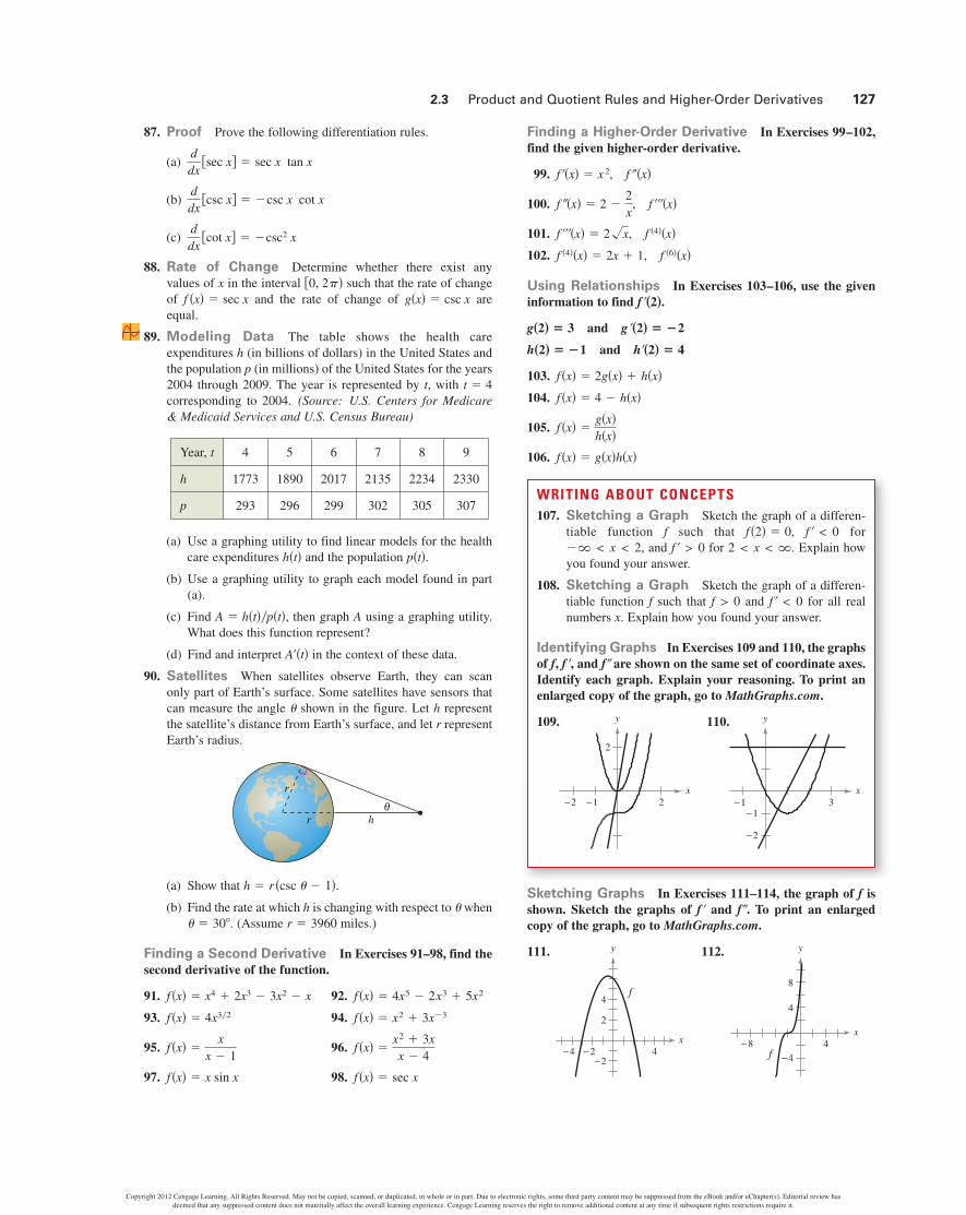
Identifying Graphs In Exercises 109 and 110, the graphsof and are shown on the same set of coordinate axes.Identify each graph. Explain your reasoning. To print anenlarged copy of the graph, go to MathGraphs.com.

109. 110.

3−1

−1

−2

x

y

2

2

−1−2x

y

ff�,f,

x.f� < 0f > 0f

2 < x < �.f� > 0�� < x < 2,f� < 0f �2� � 0,f



113. 114.

115. Acceleration The velocity of an object in meters per second is

for Find the velocity and acceleration of the objectwhen What can be said about the speed of the objectwhen the velocity and acceleration have opposite signs?

116. Acceleration The velocity of an automobile starting fromrest is

where is measured in feet per second. Find the accelerationat (a) 5 seconds, (b) 10 seconds, and (c) 20 seconds.

117. Stopping Distance A car is traveling at a rate of 66 feetper second (45 miles per hour) when the brakes are applied.The position function for the car is where is measured in feet and is measured in seconds. Usethis function to complete the table, and find the averagevelocity during each time interval.

Finding a Pattern In Exercises 119 and 120, develop a general rule for given

119. 120.

121. Finding a Pattern Consider the function

(a) Use the Product Rule to generate rules for finding and

(b) Use the results of part (a) to write a general rule for

122. Finding a Pattern Develop a general rule for where is a differentiable function of

Finding a Pattern In Exercises 123 and 124, find the derivatives of the function for 2, 3, and 4. Use theresults to write a general rule for in terms of

123. 124.

Differential Equations In Exercises 125–128, verify thatthe function satisfies the differential equation.

Function Differential Equation

125.

126.

127.

128.

True or False? In Exercises 129–134, determine whether thestatement is true or false. If it is false, explain why or give anexample that shows it is false.

129. If then

130. If then

131. If and are zero and then

132. If is an th-degree polynomial, then

133. The second derivative represents the rate of change of thefirst derivative.

134. If the velocity of an object is constant, then its acceleration iszero.

135. Absolute Value Find the derivative of Doesexist? (Hint: Rewrite the function as a piecewise

function and then differentiate each part.)

136. Think About It Let and be functions whose first andsecond derivatives exist on an interval Which of the following formulas is (are) true?

(a) (b)

137. Proof Use the Product Rule twice to prove that if andare differentiable functions of then

ddx

� f �x�g�x�h�x�� f��x�g�x�h�x� � f �x�g��x�h�x� � f �x�g�x�h��x�.

x,hg,f,

fg � f g � � fg�fg � f g � � fg� � f�g��

I.gf

f �0�f �x� � x�x�.

f �n�1��x� � 0.nf �x�h��c� � 0.h�x� � f �x�g�x�,g��c�f��c�

d5ydx5 � 0.y � �x � 1��x � 2��x � 3��x � 4�,

dydx

� f��x�g��x�.y � f �x�g�x�,

y � y � 0y � 3 cos x � sin x

y � y � 3y � 2 sin x � 3

�y� � xy � 2y� � �24x2y � 2x3 � 6x � 10

x3 y � 2x2 y� � 0y �1x, x > 0

f �x� �cos x

xnf �x� � xn sin x

n.f� x�n � 1,f

x.f�x f �x��n�,

f �n��x�.f �4��x�.f��x�,

f �x�,f �x� � g�x�h�x�.

f �x� �1x

f �x� � xn

f x�.f n� x�

tss�t� � �8.25t 2 � 66t,

v

v�t� �100t

2t � 15

t � 3.0 � t � 6.

v�t� � 36 � t 2

y

x

2

4

1

−2

−1

f

π2

π π2π2

3

y

x

234

1

−4

f

π2

π2

3

t 0 1 2 3 4

s�t�

v�t�

a�t�

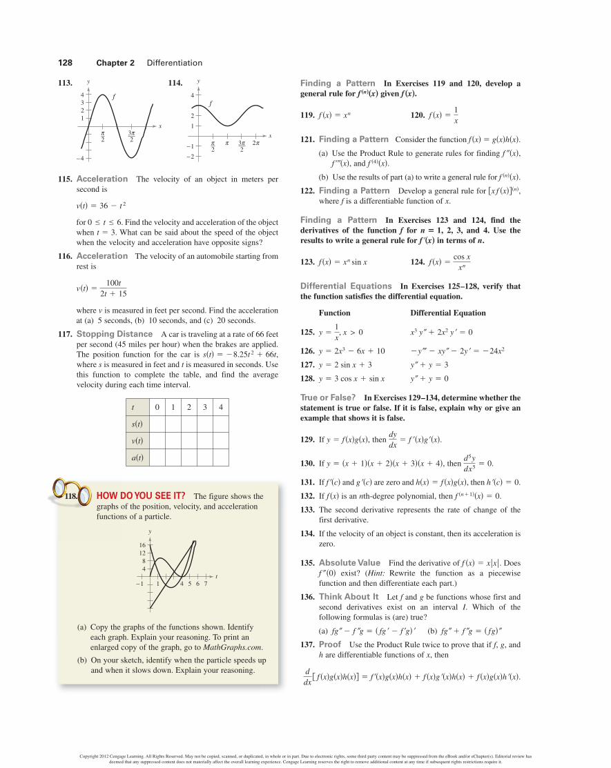
118. HOW DO YOU SEE IT? The figure shows thegraphs of the position, velocity, and accelerationfunctions of a particle.

(a) Copy the graphs of the functions shown. Identifyeach graph. Explain your reasoning. To print anenlarged copy of the graph, go to MathGraphs.com.

(b) On your sketch, identify when the particle speeds upand when it slows down. Explain your reasoning.

y

t1−1 4 5 6 7

84

1216


Section 2.3 (page 125)

1. 3.5. 7.9. 11.

13.

15. 17.

Function Rewrite Differentiate Simplify

19.

21.

23.

25. 27.

29. 31.33.35.

37. 39. t�t cos t � 2 sin t��4xc2

�x2 � c2�2

10x4 � 8x3 � 21x2 � 10x � 30��2x2 � 2x � 3��x2�x � 3�2

6s2�s3 � 2��3x � 1��2x3�2�

�x2 � 6x � 3��x � 3�23�x � 1�2, x 1

x > 0x > 0

y� �2�x

,y� � 2x�1�2y � 4x1�2,y �4x3�2

x

y� � �127x3y� � �

127

x�3y �67

x�2y �6

7x2

y� �2x � 3

7y� �

27

x �37

y �17

x2 �37

xy �x2 � 3x

7

f� �

4� ��28

�4 � ��f��1� � �14

f��x� � cos x � x sin xf��x� �x2 � 6x � 4

�x � 3�2

f��0� � �20� 15x4 � 8x3 � 21x2 � 16x � 20

f��x� � �x3 � 4x��6x � 2) � �3x2 � 2x � 5��3x2 � 4��x cos x � 2 sin x��x3�1 � 5x3��2�x�x3 � 1�2

�1 � x2��x2 � 1�2x2�3 cos x � x sin x��1 � 5t2��2�t �2�2x3 � 6x2 � 3x � 6�

Answers to Odd-Numbered Exercises A21


41.

45.

49.53.

55. 57.

59.

61.63. (a)

(b)65. (a)

(b)

69.67. (a)(b)

−4

4

−

4(π , 1 (��

2y � x � 4 � 04x � 2y � � � 2 � 0−6

1−8

8

(−5, 5)

−6

3−1

3

(1, −4)

y � 4x � 25y � �3x � 1h��t� � sec t�t tan t � 1��t2, 1�� 2

y� �

�x � 2�2

�2 csc x cot x�1 � csc x�2 , �4�3

4x cos x � �2 � x2� sin x2x2 � 8x � 1 1 � sin � � � cos �

�1 � sin ��2

51. x�x sec2 x � 2 tan x�cos x cot2 x

6 csc t cot t 47.3

sec x�tan x � sec x�2

14t3�4 �

��t sin t � cos t��t2 43. �1 � sec2 x � tan2 x

71. 73. 75.77. Tangent lines:

79. 81. (a) (b)83.85. (a)

(b)thousand�100 componentsthousand�100 components

(c) thousand�100 componentsThe cost decreases with increasing order size.

87. Proof89. (a)

(b)

(c)

represents the average health care expenditures per person (in thousands of dollars).A

20

10

10

A �112.4t � 1332

2.9t � 282

20

400

10

p(t)

20

h�t� � 112.4t � 1332p�t� � 2.9t � 2823000

10

h(t)

�$3.80�$10.37�$38.13

�18t � 5��2�t� cm2�secq��4� � �1�3p��1� � 1f �x� � 2 � g�x�

−2 22 4−2

−4

−6

6

(3, 2)(−1, 0)

2y + x = −1

2y + x = 7y

x

f (x) = x + 1 x − 1

−6 −4

2y � x � 7; 2y � x � �1�0, 0�, �2, 4��1, 1�25y � 12x � 16 � 0

(d)

represents the rate of change of the average healthcare expenditures per person for the given year t.A��t�

A��t� �27,834

8.41t2 � 1635.6t � 79,524

A22 Answers to Odd-Numbered Exercises

91. 93. 95.97. 99. 101. 103. 0

105.107. Answers will vary. 109.

Sample answer:

111. 113.

115.

The speed of the object is decreasing.117.

The average velocity on is 57.75, on is 41.25, onis 24.75, and on is 8.25.

119.121. (a)

(b)

123.

General rule: f��x� � x n cos x � nx�n�1� sin xf��x� � x 4 cos x � 4x3 sin xn � 4:f��x� � x3 cos x � 3x2 sin xn � 3:f��x� � x2 cos x � 2x sin xn � 2:f��x� � x cos x � sin xn � 1:

n!�n � 1�!1!

g�n�1��x�h��x� � g�n��x�h�x�

n!2!�n � 2�! g� �x�h�n�2��x� � . . . �

f �n��x� � g�x�h�n��x� �n!

1!�n � 1�! g��x�h�n�1��x� �

4g��x�h��x� � g�4��x�h�x�f �4��x� � g�x�h�4��x� � 4g��x�h��x� � 6g��x�h��x� �

3g� �x�h��x� � g��x�h�x�f��x� � g�x�h��x� � 3g��x�h� �x� �

f� �x� � g�x�h��x� � 2g��x�h��x� � g��x�h�x� f �n��x� � n�n � 1��n � 2� . . . �2��1� � n!

�3, 4�2, 3�1, 2�0, 1

a�3� � �6 m�sec2

v�3� � 27 m�sec

−1

−2

−3

−4

1

y

x

f ′ f ″

2π π2

−1−2−3 1 2 3 4 5

−3

−4

−5

1

2

3

4

x

y

f ′

f ″

x

1

1

2

2

3

3 4

4

y

f �x� � �x � 2�2

2

2

1

1−1−2x

f

y

f ′

f ″

�101��x2x2 cos x � x sin x

2��x � 1�33��x12x2 � 12x � 6

t 0 1 2 3 4

s�t� 0 57.75 99 123.75 132

v�t� 66 49.5 33 16.5 0

a�t� �16.5 �16.5 �16.5 �16.5 �16.5


125.

127.

129. 131. True133. True 135. does not exist.137. Proof

f � �0�f��x� � 2�x�;

y� � 2 cos x, y� � �2 sin x,y� � y � �2 sin x � 2 sin x � 3 � 3False. dy�dx � f �x�g��x� � g�x�f��x�

� 2 � 2 � 0

y� � �1�x2, y� � 2�x3, x3y� � 2x2y� � x3�2�x3� � 2x2��1�x2�

Documents

Chapter 2 Differentiation 2.3 Product and Quotient Rules