Chapter 16 – Processing of Transmission Electron

HAL Id: hal-01430532https://hal.archives-ouvertes.fr/hal-01430532

Submitted on 10 Jan 2017

HAL is a multi-disciplinary open accessarchive for the deposit and dissemination of sci-entific research documents, whether they are pub-lished or not. The documents may come fromteaching and research institutions in France orabroad, or from public or private research centers.

L’archive ouverte pluridisciplinaire HAL, estdestinée au dépôt et à la diffusion de documentsscientifiques de niveau recherche, publiés ou non,émanant des établissements d’enseignement et derecherche français ou étrangers, des laboratoirespublics ou privés.

Processing of Transmission Electron Microscopy Imagesfor Single-Particle Analysis of Macromolecular

ComplexesZaelle Devaux, Carlos Oscar S. Sorzano, Slavica Jonic

To cite this version:Zaelle Devaux, Carlos Oscar S. Sorzano, Slavica Jonic. Processing of Transmission Electron Mi-croscopy Images for Single-Particle Analysis of Macromolecular Complexes. Methods in Cell Biology,Elsevier, 2012, 112, pp.295-310. �10.1016/B978-0-12-405914-6.00016-0�. �hal-01430532�

https://hal.archives-ouvertes.fr/hal-01430532

https://hal.archives-ouvertes.fr

295Methods in Cell Biology, Vol 112 Copyright © 2012 Elsevier Inc. All rights reserved.

0091-679Xhttp://dx.doi.org/10.1016/B978-0-12-405914-6.00016-0

Zaelle Devaux*, Carlos Oscar S. Sorzano†, Slavica Jonic*,1

*IMPMC, UMR 7590, CNRS-Université Pierre and Marie Curie-IRD, Campus Jussieu,

Paris Cedex 05, France†Biocomputing Unit, Centro Nacional de Biotecnología—CSIC,

Campus de Cantoblanco, Madrid, Spain1Corresponding author: [email protected]

CHAPTER

Processing of Transmission Electron Microscopy Images for Single-Particle Analysis of Macromolecular Complexes

16

CHAPTER OUTLINE

1 Purpose ............................................................................................................... 2962 Theory ................................................................................................................. 2963 Equipment ........................................................................................................... 2994 Materials ............................................................................................................. 2995 Protocol .............................................................................................................. 301

5.1 Step 1—Screen Micrographs and Estimate the CTF Parameters ..............3025.2 Step 2—Pick and Screen Particles .......................................................3035.3 Step 3—Create Defocus Groups and Prepare

the First Reference Volume ..................................................................3055.4 Step 4—Refine Iteratively the 3D Structure by Projection Matching

with CTF Correction ............................................................................305

AbstractThree-dimensional (3D) structure of a wide range of biological macromolecular assemblies can be computed from two-dimensional images collected by transmission electron microscopy. This information integrated with other structural data (e.g., from X-ray crystallography or nuclear magnetic resonance) helps structural biolo-gists understand the function of macromolecular complexes. Single-particle analysis (SPA) is a method used for studies of complexes whose structure and dynamics can be analyzed in isolation. To reconstruct the 3D structure, SPA methods use a large number of images of randomly oriented individual complexes. When the angular

CHAPTER 16 Processing of Transmission Electron Microscopy Images296

distribution of single-particle orientations samples Fourier space completely and the population is structurally homogeneous, a resolution of the reconstruction of 0.4-1 nm can be achieved. Such high resolutions are possible thanks to the high number of images and the correction of the Contrast Transfer Function (CTF) of the micro-scope. One of the standard SPA approaches is the refinement of a preliminary 3D model using iterative projection matching combined with CTF correction. We describe a protocol for the refinement of a preliminary model using CTF correction by Wiener filtering of volumes from focal series of experimental images. This proto-col combines potentially best features of two other protocols proposed in the field.

1 PURPOSEThe purpose of this protocol is to compute a three-dimensional structure of a macromo-lecular complex by single-particle analysis of transmission electron microscopy images.

2 THEORYThree-dimensional (3D) structure of a widerange of biological macromolecular assem-blies can be computed from two-dimensional (2D) images collected by transmission electron microscopy. This information integrated with other structural data (e.g. from X-ray crystallography) helps structural biologists understand the function of macromo-lecular complexes. Single-particle analysis (SPA) is a method used for studies of macro-molecular assemblies whose structure and dynamics can be analyzed in isolation (e.g. proteins, ribosomes, viruses) (Frank 2006; Jonic et al., 2008; jonic and Venien-Bryan, 2009). It is complementary to nuclear magnetic resonance since it allows computing the structure of large assemblies (diameter of 10–30 nm). It is also complementary to X-ray crystallography since it allows studying noncrystalline matter.

To reconstruct the 3D structure, SPA methods use a large number of images of ran-domly oriented individual molecules (Fig. 1). In practice, the analysis requires images of thousands of individual molecules of the same protein captured in a unique confor-mation taken in random orientation. Note that we do not treat, in this protocol, the case of the samples with structural heterogeneity (for a review on this topic, see Leschziner & Nogales, 2007). When the angular distribution of single-particle orientations samples Fourier space completely and the population is structurally homogeneous, standard image processing strategies allow computing an average structure at resolution of 0.4–1 nm (Connell et al., 2007; Cottevieille et al., 2008; Ludtke et al., 2008; Venien-Bryan et al., 2009; Zhang et al., 2008). Such high resolutions are possible thanks to a high number of images used for 3D reconstruction and the correction of the contrast transfer function (CTF) of the microscope. The CTF is expressed in reciprocal space and its equivalent in real space is termed point spread function as it describes how the image of a single point is spread into a diffused spot because of the imperfections of the electron microscope (e.g. spherical and chromatic aberrations, instabilities of magnetic lenses, instabilities of electron acceleration, additive noise, drift or charging).

2 Theory 297

One of the standard SPA methods is the refinement of a preliminary 3D model using iterative projection matching combined with CTF correction. An already solved structure from the same family of macromolecular complexes can be down-loaded from the PDB database (http://www.ebi.ac.uk/pdbe/) or the EMDB database (http://www.ebi.ac.uk/pdbe/emdb/) and used as the preliminary model, after an appropriate low-pass filtering to remove fine structural details, and thus prevent bias-ing the outcome by the high-resolution features in the initial reference (Fig. 2). If such structure is not available, other techniques can help obtain the preliminary model (e.g. random conical tilt series (Radermacher, 1988), common lines (Penczek, Zhu, & Frank, 1996)). Here, we describe a protocol for the refinement of a prelimi-nary PDB or EMDB model using CTF correction by Wiener filtering of volumes from focal series of experimental images (Penczek, Zhu, Schröder, & Frank, 1997) thanks to which we obtained several low-symmetry structures at subnanometer reso-lution (Cottevieille et al., 2008; Venien-Bryan et al., 2009). This protocol is inspired by two from several protocols proposed in the field (Scheres, Nunez-Ramirez, Sorzano, Carazo, & Marabini, 2008; Shaikh et al., 2008) and aims at combining potentially best features of both.

The experimental images to be used for reconstruction are first screened on two levels. On the micrograph level, the screening is done to detect and reject micro-graphs with important information loss (e.g. due to thermal drift effects) or high

FIGURE 1

Area of a micrograph containing hundreds of single particles (squares) in random and unknown orientations. See the color plate.

http://www.ebi.ac.uk/pdbe/

http://www.ebi.ac.uk/pdbe/emdb/


astigmatism in case of Wiener filtering of volumes from focal series (Jonic, Sorzano, Cottevieille, Larquet, & Boisset, 2007) (Fig. 3). At the same time, the CTF parame-ters are estimated for each micrograph (Sorzano et al., 2007) (Fig. 4). On the level of isolated single-particle images, the classification is done to detect and reject the images containing the structures inconsistent with the structure of the remaining par-ticles (Sorzano et al., 2010) (Fig. 5).

The kept single particles are classified into groups containing images with simi-lar defocus values. For each defocus group, the 3D defocus-group CTF is applied on the 3D reference. The CTF affected volume is then projected using known projec-tion directions (known angular sampling step) to compute a library of 2D reference projections with known orientations. The experimental single-particle images are then correlated with the reference projections (projection matching of the 3D refer-ence with experimental images) to compute roughly the orientation of the experi-mental images (Jonic et al., 2005; Sorzano et al., 2004). The oriented images in each defocus group are used for the 3D reconstruction of the corresponding defocus-group volume and the volumes are merged using a Wiener filter computed for the defocus-groups CTF parameters (Penczek et al., 1997). Until the resolution of the reconstructed structure becomes stable (Fig. 6), this merged CTF-corrected volume is used as the refined 3D reference for the next iteration, in which the projection matching is performed with the reference projections computed for a smaller angu-lar sampling step.

FIGURE 2

Two views of the structure of the ribosomal subunit 30S of T. thermophilus downloaded from the Protein Data Bank (PDB code: 1j5e), low-pass filtered, and used as the prelimi-nary model for 3D reconstruction of the subunit 30S of P. abyssi.

3 Equipment 299

FIGURE 3

Screening of micrographs to detect thermal drift effects and astigmatism. Top panels: power spectral density of experimental images, with masked very low frequencies to improve the visibility of contrast transfer function rings. Bottom panels: band-pass filtered power spectral densities to improve the rings visibility, with masked very low and very high frequencies. Left panels: rings circularly symmetric (absence of astigmatism). Right panels: rings visible only in one direction (thermal drift).

3 EQUIPMENTDesktop PC with multiple processing cores or a cluster.

4 MATERIALSLinux operating systemSPA software Xmipp (http://xmipp.cnb.csic.es) or Spider (http://www.wadsworth.org/spider_doc)2D visualization software (e.g. provided by SPA package)3D visualization software (e.g. Chimera (http://www.cgl.ucsf.edu/chimera))

http://xmipp.cnb.csic.es

http://www.wadsworth.org/spider_doc

http://www.wadsworth.org/spider_doc

http://www.cgl.ucsf.edu/chimera


FIGURE 4

Combined image composed of the left half of the band-pass filtered power spectral density and the right half of the estimated two-dimensional contrast transfer function to check the accuracy of the estimation of the contrast transfer function.

FIGURE 5

Screening of single particle images to detect heterogeneity. Classification of around 10,000 single particles in 50 classes, considered as homogeneous. Class averages with the number of particles indicated for each class.

5 Protocol 301

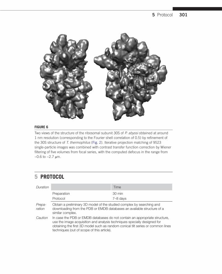
FIGURE 6

Two views of the structure of the ribosomal subunit 30S of P. abyssi obtained at around 1 nm resolution (corresponding to the Fourier shell correlation of 0.5) by refinement of the 30S structure of T. thermophilus (Fig. 2). Iterative projection matching of 9523 single-particle images was combined with contrast transfer function correction by Wiener filtering of five volumes from focal series, with the computed defocus in the range from −0.6 to −2.7 μm.

5 PROTOCOL

Duration Time

Preparation 30 minProtocol 7–8 days

Prepa-ration

Obtain a preliminary 3D model of the studied complex by searching and downloading from the PDB or EMDB databases an available structure of a similar complex.

Caution In case the PDB or EMDB databases do not contain an appropriate structure, use the image acquisition and analysis techniques specially designed for obtaining the first 3D model such as random conical tilt series or common lines techniques (out of scope of this article).


Tip Duration reported here includes both computing time and time for various intermediate results analyses. Computing time can be reduced with a higher number of processing cores. Duration reported here is for the use of 32 cores at maximum, intermediate resolution of 3D reconstruction (∼1.5 nm), interme-diate-size data set (100 micrographs with a total of about 10,000 particles and the particle size of 128 × 128 pixels), and particles of asymmetric form. Required time would be shorter for highly symmetric structures since their reconstruction requires less data to be analyzed for the same target resolution (e.g. icosahedral viruses). Larger the data size, longer the duration but better the resolution of the reconstruction.

See Fig. 7 for the flowchart of the complete protocol.

5.1 Step 1—Screen Micrographs and Estimate the CTF Parameters

Overview Screen micrographs to detect and reject micrographs with important information loss (e.g. due to thermal drift effects) and high astigmatism, and estimate the CTF for kept micrographs.

Duration About 3 h.1.1 Compute 2D power spectrum density (PSD) for each micrograph.1.2 Compute band-pass filtered PSDs to improve the visibility of the

CTF-related rings.1.3 Detect the PSDs with the CTF-related rings with significant circular

asymmetry.1.4 Remove micrographs giving anisotropic PSDs.1.5 Compute the CTF parameters for kept micrographs after Step 1.4.1.6 Visualize a combined image composed of the left half of the band-pass

filtered PSD and the right half of the estimated two-dimensional CTF (Fig. 4).

Preparation

Step 1

Step 2

Step 4

Obtain a preliminary 3D model by searching and downloading from the PDB or EMDB databases an available structure of a similar complex. Otherwise, use the image acquisition and analysis techniques such as random conical tilt series or common lines techniques.

Screen micrographs and estimate the CTF parameters

Pick and screen particles

Refine iteratively the 3D structure by projection matching with CTF correction

Create defocus groups and prepare the first reference volumeStep 3

FIGURE 7

Flowchart of the complete protocol, including preparation.

5 Protocol 303

1.7 Compare the left and right sides of the combined image in Step 1.6 to check the accuracy of the CTF estimation.

1.8 For the micrographs with inaccurate CTF estimation, recompute the CTF by local refinement of given values for the defocus parameters and repeat Steps 1.6 and 1.7 until a successful CTF estimation.

1.9 Keep only the micrographs giving good correspondence between the left and right sides in the combined image in Step 1.6 and keep the corre-sponding estimated CTF parameters.

1.10 Flip phase of micrographs using computed CTF parameters.Caution Micrographs can be slightly tilted, which results in different CTF param-

eters over different areas of the same micrograph.Tip To avoid mixing particles with very different defocus values, split each

micrograph into areas and perform Steps 1.1–1.10 locally (on micrograph’s areas instead of analyzing entire micrographs).

See Fig. 8 for the flowchart of Step 1.

5.2 Step 2—Pick and Screen Particles

Overview Isolate particles from micrographs in separate images and detect and keep only structurally homogeneous set of particles.

Duration About 4 days.2.1 Pick several particles using different box sizes (in pixels) and choose the

size of the box that can contain the entire particle.

Step 1Screen micrographs and estimate the CTF parameters

1.1 Compute two-dimensional power spectrum density (PSD) for each micrograph

1.2 Compute band-pass filtered PSDs to improve the visibility of the CTF-related rings

1.3 Detect the PSDs with the CTF-related rings with significant circular asymmetry

1.5 Compute the CTF parameters for kept micrographs after 1.4

1.4 Remove micrographs giving anisotropic PSDs

1.6 Visualize a combined image composed of the left half of the band-pass filtered PSD and the right half of the estimated two-dimensional CTF (Figure 4)

1.7 Check two sides of the combined image in 1.6 for accuracy of the CTF estimation

1.8 For the micrographs with inaccurate CTF estimation, re compute the CTF by local refinement of given values for the defocus parameters and repeat 1.6 and 1.7

1.9 Keep only the micrographs giving good correspondence between two sides of the combined image in 1.6 and keep the corresponding estimated CTF parameters

1.10 Flip phase of micrographs using computed CTF parameters

FIGURE 8

Flowchart of Step 1.


2.2 Pick particles semiautomatically using the box size selected in Step 2.1 and store the picked box coordinates.

2.3 Visualize and correct the results of the automatic picking by detecting and rejecting the boxes not containing particles and by picking the missed particles.

2.4 Extract the particles from micrographs using the stored box coordinates.

2.5 Normalize the particles so that the mean and the standard deviation are constant over the series.

2.6 Invert the contrast in case of “black” particles on “white” background.2.7 Perform classifications of picked particles with different number of

classes.2.8 Visualize the class averages and the individual particles in each class.2.9 Reject the classes inconsistent with the rest of the classes (produce the

final set of particles to be used in the next step).Tip You can pick the particles using any of the software packages special-

ized for SPA since each of them contains an interactive graphical interface for semiautomatic particle boxing and inspection of boxed particles.


Step 2Pick and screen particles

2.1 Pick several particles with different box sizes and choose the appropriate size

2.2 Pick particles semi automatically with the selected box size and store the coordinates

2.3 Visualize and correct the results of the automatic picking by detecting and rejecting the boxes not containing particles and by picking the missed particles

2.4 Extract the particles from micrographs using the stored box coordinates

2.5 Normalize the particles (mean and standard deviation to be constant over the series)

2.6 Invert the contrast in case of “black” particles on “white” background

2.8 Visualize the class averages and the individual particles in each class

2.9 Reject the classes inconsistent with the rest of the classes (produce the final set of particles to be used in the next step)

2.7 Perform classifications of picked particles with different number of classes

FIGURE 9


5 Protocol 305

5.3 Step 3—Create Defocus Groups and Prepare the First Reference Volume

Overview Create groups of particles with similar defocus values (defocus groups) and process the available preliminary 3D model to adapt it to the scale of the extracted particle images and remove as much as possible the structural details.

Duration About 3 h3.1 Split particles into defocus groups for several given values of the

maximum defocus difference in each group.3.2 Check the number of particles per defocus group and select the split

results corresponding to the maximum defocus difference producing the majority of groups with a high number of particles per group (e.g. at least 1000 particles in case of asymmetric structures).

3.3 Check the number of particles per defocus group in the split results selected in Step 3.2 and either remove the groups with small number of particles or merge small groups into larger groups, so that all defocus groups have comparable number of particles.

3.4 Compute the volumetric CTF using the mean defocus value for each defocus group (group CTFs).

3.5 Build the reference volume from the preliminary 3D model by rescaling the corresponding density volume, so that its pixel size is that of the particle image and the volume dimension is N3 for the particle image size of N2 pixels.

3.6 Low-pass filter the volume as much as possible.Caution Reference-based procedures are sensitive to reference bias.Tip To avoid biasing of the output with the high-resolution features of the

initial volume, low-pass filter the volume in Step 3.6 as much as possible (0.3–0.6 nm resolution may be required as the cutoff). In addition, it is a good practice to perform independent reconstructions using two (or more) different initial volumes.


5.4 Step 4—Refine Iteratively the 3D Structure by Projection Matching with CTF Correction

Overview Images are processed by defocus groups. The projection matching is done in each defocus group with the group CTF applied on the 3D reference. The oriented images in each defocus group are then used to compute one 3D volume per group. The 3D CTF correction is done by merging the volumes from different groups by Wiener filtering and the merged volume is used as the 3D reference for the next iteration.

Duration About 3 days.4.1 For each defocus group, apply the group CTF on the reference

volume.


4.2 For each defocus group, project the obtained group volume using known projection directions to compute a gallery of reference projections.

4.3 For each defocus group, compute the particle orientation and shift by matching experimental images with the reference projections.

4.4 For each defocus group, perform a 2D realignment of images assigned to each reference projection direction to remove model bias from the refinement procedure.

4.5 For each defocus group, compute a 3D reconstruction with the aligned images.

4.6 Compute the iteration volume by Wiener filtering of the series of group volumes.

4.7 Estimate the resolution limit of the iteration volume by Fourier Shell Correlation of two “half”-volumes (reconstructed from two randomly selected halves of the image series and masked to remove noise around the structure).

4.8 Low-pass filter the iteration volume at the estimated resolution (or a little less to avoid overfitting) and mask it to remove noise around the structure.

Step 3Create defocus groups and prepare the first reference volume

3.1 Split particles into defocus groups for several given values of the maximum defocus difference in each group

3.4 Compute the volumetric CTF using the mean defocus value for each defocus group (group CTFs)

3.2 Check the number of particles per defocus group and select the split results producing the majority of groups with a high number of particles per group (e.g. at least 1000 particles in case of asymmetric structures)

3.3 Check the number of particles per defocus group in the split results selected in 3.2 and either remove the groups with small number of particles or merge small groups into larger groups so that all groups have comparable number of particles

3.5 Build the reference volume from the preliminary 3D model by rescaling the corresponding density volume so that its pixel size is that of the particle image and the volume dimension is N3 for the particle image size of N2 pixels.

3.6 Low-pass filter the volume as much as possible

FIGURE 10


5 Protocol 307

4.9 Repeat the Steps 4.1–4.8 using the latest iteration volume as the reference volume and reducing the angular step for reference projections computation, until the resolution does not improve anymore.

Caution Mask should be a binary mask with smooth edges (low-pass filter the edges of a binary mask). The mask should not be too small (the mask and structure edges should not be too close to each other).

Tip Start by performing several iterations of the volume refinement without modifying the iteration volume (skip the Steps 4.7 and 4.8). Only after obtaining a volume with significantly reduced noise, create a binary mask that corresponds to the shape of the obtained structure (using several iterations of a combined thresholding and low-pass filtering until the mask of a suitable size is obtained). Then, low-pass filter the edges of the mask and continue the refinement without skipping the Steps 4.7 and 4.8.


Step 4Refine iteratively the 3D structure by projection matching with CTF correction

4.1 For each defocus group, apply the group CTF on the reference volume

4.2 For each defocus group, project the obtained group volume using known projection directions to compute a gallery of reference projections

4.3 For each defocus group, compute the particle orientation and shift by matching experimental images with the reference projections

4.5 For each defocus group, compute a 3D reconstruction with the aligned images

4.4 For each defocus group, perform a 2D re alignment of images assigned to each reference projection direction to remove model bias from the refinement procedure

4.6 Compute the iteration volume by Wiener filtering of the series of group volumes

4.7 Estimate the volume resolution by Fourier Shell Correlation of two masked “half”-volumes

4.8 Low-pass filter the iteration volume at the estimated resolution (or a little less to avoid overfitting) and mask it to remove noise around the structure

4.9 Repeat the steps 4.1 to 4.8 using the latest iteration volume as the reference volume and reducing the angular step for reference projections computation, until the resolution does not improve anymore

FIGURE 11



Keywords

Keyword Class Keyword Rank Snippet

MethodsList the methods used to carry out this protocol (i.e. for each step).

1. Image classification

Used to select structurally homogeneous set of images

2. Image alignment Used to compute orientation and translation of images with respect to a reference

3. Three- dimensional (3D) reconstruction

Used to compute 3D structure from 2D images

4. Wiener filter Used to correct contrast transfer function of the microscope

5. Single particle analysis

Used to compute an average structure of a complex from a high number of individual particles images

ProcessList the biological process(es) addressed in this protocol.

12345

OrganismsList the primary organism used in this protocol. List any other applicable organisms.

12345

PathwaysList any signaling, regulatory, or metabolic pathways addressed in this protocol.

12345

Molecule rolesList any cellular or molecular roles addressed in this protocol.

12345

Molecule functionsList any cellular or molecular functions or activities addressed in this protocol.

12345

PhenotypeList any developmental or functional phenotypes addressed in this protocol (organismal or cellular level).

12345

5 Protocol 309

Keyword Class Keyword Rank Snippet

AnatomyList any gross anatomical structures, cellular structures, organelles, or macromolecular com-plexes pertinent to this protocol.

12345

DiseasesList any diseases or disease processes addressed in this protocol.

12345

OtherList any other miscella-neous keywords that describe this protocol.

12345

AcknowledgmentsWe thank the team of Dr Yves Méchulam (Ecole polytechnique, Palaiseau, France) for provid-ing us with the biological samples used for illustrating this article, to the ANR (ANR-06-PCVI-0018-01, ANR-11-BSV8-010-04), the CNRS and the CSIC (PICS 2011 “4DTEMmol”) for supporting our research, and to GENCI-CINES/IDRIS for using HPC resources (2010-x2010072174, 2011-x2010072174, 2012-x2011072174).

ReferencesSource article(s) used to create this protocolJonic, S., Sorzano, C. O., & Boisset, N. (2008). Comparison of single-particle analysis and

electron tomography approaches: an overview. Journal of Microscopy, 232, 562–579.Jonic, S., & Venien-Bryan, C. (2009). Protein structure determination by electron cryo-

microscopy. Current Opinion in Pharmacology, 9, 636–642.Sorzano, C. O., Jonic, S., Cottevieille, M., Larquet, E., Boisset, N., & Marco, S. (2007). 3D

electron microscopy of biological nanomachines: principles and applications. European Biophysics Journal, 36, 995–1013.

Sorzano, C. O. S., de la Rosa Trevín, J. M., Otón, J., Vega, J. J., Cuenca, J., Zaldívar-Peraza, A., et al. Semiautomatic, high-throughput, high-resolution protocol for three-dimensional reconstruction of single particles in electron microscopy. In S. Alioscka & K. Michael (Eds.), Nanoimaging: Methods and protocols. Humana Press, (in press).

Referenced literatureConnell, S. R., Takemoto, C., Wilson, D. N., Wang, H., Murayama, K., Terada, T., et al. (2007).

Structural basis for interaction of the ribosome with the switch regions of GTP-bound elongation factors. Molecular Cell, 25, 751–764.


Cottevieille, M., Larquet, E., Jonic, S., Petoukhov, M. V., Caprini, G., Paravisi, S., et al. (2008). The subnanometer resolution structure of the glutamate synthase 1.2-MDa hexamer by cryoelectron microscopy and its oligomerization behavior in solution: functional implica-tions. Journal of Biological Chemistry, 283, 8237–8249.

Jonic, S., Sorzano, C. O., Thevenaz, P., El-Bez, C., De Carlo, S., & Unser, M. (2005). Spline-based image-to-volume registration for three-dimensional electron microscopy. Ultrami-croscopy, 103, 303–317.

Jonic, S., Sorzano, C. O., Cottevieille, M., Larquet, E., & Boisset, N. (2007). A novel method for improvement of visualization of power spectra for sorting cryo-electron micrographs and their local areas. Journal of Structural Biology, 157, 156–167.

Leschziner, A. E., & Nogales, E. (2007). Visualizing flexibility at molecular resolution: analy-sis of heterogeneity in single-particle electron microscopy reconstructions. Annual Review of Biophysics and Biomolecular Structure, 36, 43–62.

Ludtke, S. J., Baker, M. L., Chen, D. H., Song, J. L., Chuang, D. T., & Chiu, W. (2008). De novo backbone trace of GroEL from single particle electron cryomicroscopy. Structure, 16, 441–448.

Penczek, P. A., Zhu, J., & Frank, J. (1996). A common-lines based method for determining orientations for N > 3 particle projections simultaneously. Ultramicroscopy, 63, 205–218.

Penczek, P. A., Zhu, J., Schröder, R., & Frank, J. (1997). Three dimensional reconstruction with contrast transfer compensation from defocus series. Scanning Microscopy, 11, 147–154.

Radermacher, M. (1988). Three-dimensional reconstruction of single particles from random and nonrandom tilt series. Journal of Electron Microscopy Technique, 9, 359–394.

Scheres, S. H., Nunez-Ramirez, R., Sorzano, C. O., Carazo, J. M., & Marabini, R. (2008). Image processing for electron microscopy single-particle analysis using XMIPP. Nature Protocols, 3, 977–990.

Shaikh, T. R., Gao, H., Baxter, W. T., Asturias, F. J., Boisset, N., Leith, A., & Frank, J. (2008). SPIDER image processing for single-particle reconstruction of biological macromolecules from electron micrographs. Nature Protocols, 3, 1941–1974.

Sorzano, C. O., Jonic, S., El-Bez, C., Carazo, J. M., De Carlo, S., Thevenaz, P., et al. (2004). A multiresolution approach to orientation assignment in 3D electron microscopy of single particles. Journal of Structural Biology, 146, 381–392.

Sorzano, C. O., Jonic, S., Nunez-Ramirez, R., Boisset, N., & Carazo, J. M. (2007). Fast, robust, and accurate determination of transmission electron microscopy contrast transfer function. Journal of Structural Biology, 160, 249–262.

Sorzano, C. O., Bilbao-Castro, J. R., Shkolnisky, Y., Alcorlo, M., Melero, R., Caffarena- Fernandez, G., et al. (2010). A clustering approach to multireference alignment of single-particle projections in electron microscopy. Journal of Structural Biology, 171, 197–206.

Venien-Bryan, C., Jonic, S., Skamnaki, V., Brown, N., Bischler, N., Oikonomakos, N. G., et al. (2009). The structure of phosphorylase kinase holoenzyme at 9.9 Å resolution and location of the catalytic subunit and the substrate glycogen phosphorylase. Structure, 17, 117–127.

Zhang, X., Settembre, E., Xu, C., Dormitzer, P. R., Bellamy, R., Harrison, S. C., et al. (2008). Near-atomic resolution using electron cryomicroscopy and single-particle reconstruction. Proceedings of the National Academy of Sciences of the United States of America, 105, 1867–1872.

Related literatureFrank, J. (2006). Three-dimensional electron microscopy of macromolecular assemblies: Visu-

alization of biological molecules in their native state. New York: Oxford University Press.

Documents

Chapter 16 – Processing of Transmission Electron