Chapter 16

Numerical Integration Formulas

Gab-Byung Chae

2007�̧� 11�Z4 4{9�

2

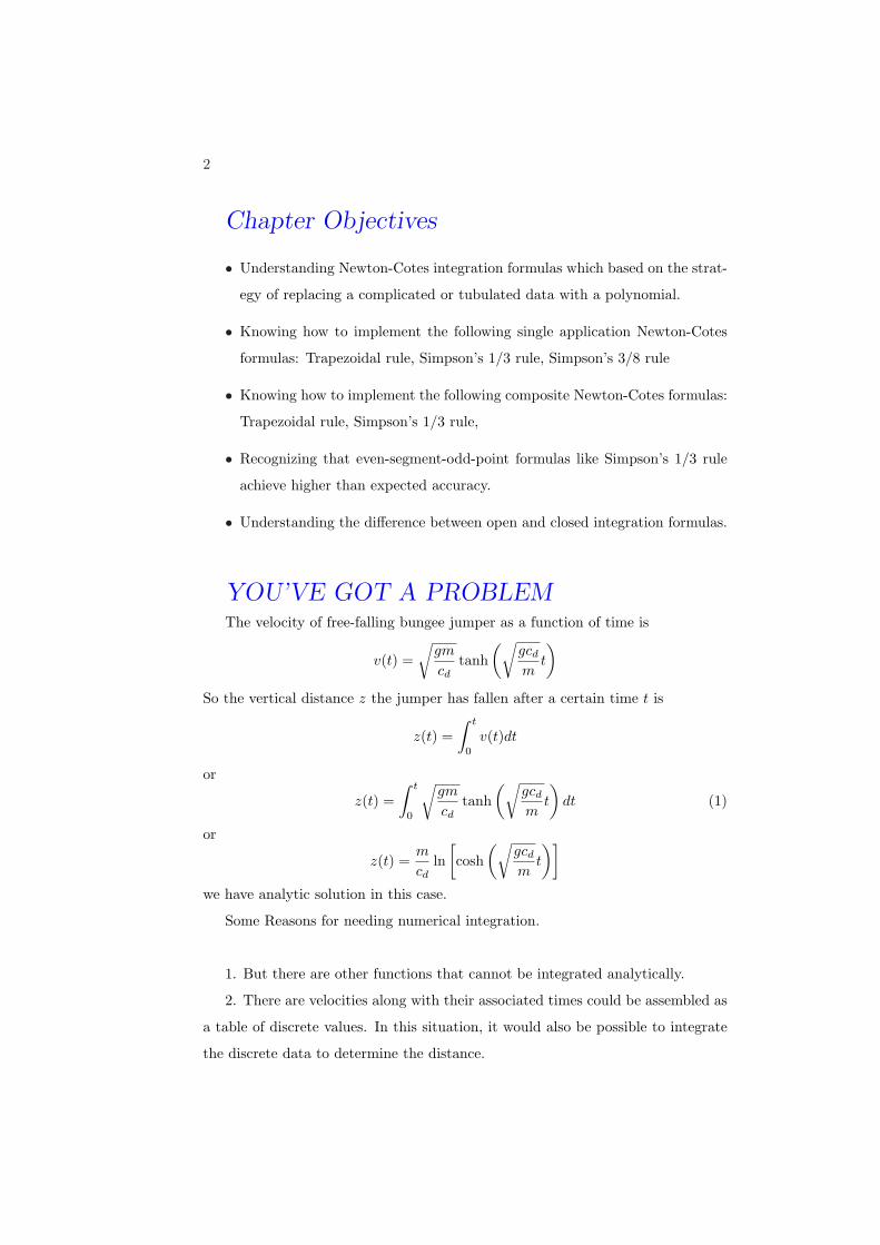
Chapter Objectives

• Understanding Newton-Cotes integration formulas which based on the strat-

egy of replacing a complicated or tubulated data with a polynomial.

• Knowing how to implement the following single application Newton-Cotes

formulas: Trapezoidal rule, Simpson’s 1/3 rule, Simpson’s 3/8 rule

• Knowing how to implement the following composite Newton-Cotes formulas:

Trapezoidal rule, Simpson’s 1/3 rule,

• Recognizing that even-segment-odd-point formulas like Simpson’s 1/3 rule

achieve higher than expected accuracy.

• Understanding the difference between open and closed integration formulas.

YOU’VE GOT A PROBLEMThe velocity of free-falling bungee jumper as a function of time is

v(t) =√

gm

cdtanh

(√gcd

mt

)

So the vertical distance z the jumper has fallen after a certain time t is

z(t) =∫ t

0

v(t)dt

or

z(t) =∫ t

0

√gm

cdtanh

(√gcd

mt

)dt (1)

or

z(t) =m

cdln

[cosh

(√gcd

mt

)]

we have analytic solution in this case.

Some Reasons for needing numerical integration.

1. But there are other functions that cannot be integrated analytically.

2. There are velocities along with their associated times could be assembled as

a table of discrete values. In this situation, it would also be possible to integrate

the discrete data to determine the distance.

3

INTRODUCTION AND BACKGROUNDWhat is Integration?

I =∫ b

a

f(x)dx

is the total value, or summation, of f(x)dx over the range x = a to b. For functions

lying above the x axis, the integral corresponds to the area under the curve of f(x)

between x = a and b.

Integration in Engineering and Science

Mean

Mean =∑n

i=1 yi

n: discrete case

Mean =

∫ b

af(x)dx

b− a: continuous case

Integrals are also employed by engineers and scientists to evaluate the total

amount or quantity of a given physical variable.

For example:

Mass = concentration × volume

If the concentration varies from location to location, it is necessary to sum the

products of local concentrations ci and corresponding elemental volumes ∆Vi :

Mass =n∑

i=1

ci∆Vi : discrete case

where n is the number of discrete volumes.

Mean =∫∫∫

c(x, y, z)dxdydz : continuous case

or

Mean =∫∫∫

V

c(V )dV

where c(x, y, z) is a known concentration function and x, y, and z are independent

variables designating position in Cartesian coordinates.

The total rate of energy transfer across a plane where the flux(rate of energy

per unit area) is a function of position is given by

Flux =∫∫

A

flux dA

4

NEWTON-COTES FORMULASThe Newton-Cotes formulas are based on the strategy of replacing a compli-

cated function or tabulated data with a polynomial that is easy to integrate:

I =∫ b

a

f(x)dx ∼=∫ b

a

fn(x)dx (2)

where fn(x) = a polynomial of the form

fn(x) = a0 + a1x + · · ·+ an−1xn−1 + anxn

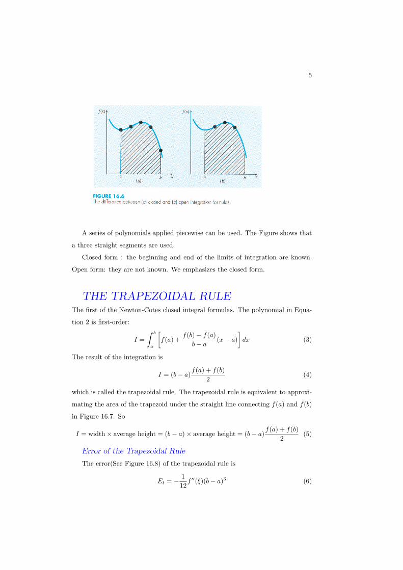
A first-order polynomial is used as an approximation(left). A parabola is used

for same purpose.(right).

5

A series of polynomials applied piecewise can be used. The Figure shows that

a three straight segments are used.

Closed form : the beginning and end of the limits of integration are known.

Open form: they are not known. We emphasizes the closed form.

THE TRAPEZOIDAL RULEThe first of the Newton-Cotes closed integral formulas. The polynomial in Equa-

tion 2 is first-order:

I =∫ b

a

[f(a) +

f(b)− f(a)b− a

(x− a)]

dx (3)

The result of the integration is

I = (b− a)f(a) + f(b)

2(4)

which is called the trapezoidal rule. The trapezoidal rule is equivalent to approxi-

mating the area of the trapezoid under the straight line connecting f(a) and f(b)

in Figure 16.7. So

I = width× average height = (b− a)× average height = (b− a)f(a) + f(b)

2(5)

Error of the Trapezoidal Rule

The error(See Figure 16.8) of the trapezoidal rule is

Et = − 112

f ′′(ξ)(b− a)3 (6)

6

where ξ lies somewhere in the interval from a to b.

If a function is linear Et = 0.

¨ Example 0.1 Use Equation 4 to numerically integrate

f(x) = 0.2 + 25x− 200x2 + 675x3 − 900x4 + 400x5

from a = 0 to b = 0.8. The exact value is 1.640533.

Solution

7

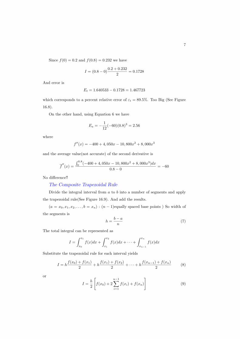
Since f(0) = 0.2 and f(0.8) = 0.232 we have

I = (0.8− 0)0.2 + 0.232

2= 0.1728

And error is

Et = 1.640533− 0.1728 = 1.467723

which corresponds to a percent relative error of εt = 89.5%. Too Big (See Figure

16.8).

On the other hand, using Equation 6 we have

Ea = − 112

(−60)(0.8)3 = 2.56

where

f ′′(x) = −400 + 4, 050x− 10, 800x2 + 8, 000x3

and the average value(not accurate) of the second derivative is

f′′(x) =

∫ 0.8

0(−400 + 4, 050x− 10, 800x2 + 8, 000x3)dx

0.8− 0= −60

No difference!!

The Composite Trapezoidal Rule

Divide the integral interval from a to b into a number of segments and apply

the trapezoidal rule(See Figure 16.9). And add the results.

(a = x0, x1, x2, . . . , b = xn) : (n − 1)equally spaced base points ) So width of

the segments is

h =b− a

n(7)

The total integral can be represented as

I =∫ x1

x0

f(x)dx +∫ x2

x1

f(x)dx + · · ·+∫ xn

xn−1

f(x)dx

Substitute the trapezoidal rule for each interval yields

I = hf(x0) + f(x1)

2+ h

f(x1) + f(x2)2

+ · · ·+ hf(xn−1) + f(xn)

2(8)

or

I =h

2

[f(x0) + 2

n−1∑

i=1

f(xi) + f(xn)

](9)

8

or, by Equation 7,

I = (b− a)︸ ︷︷ ︸width

f(x0) + 2∑n−1

i=1 f(xi) + f(xn)2n︸ ︷︷ ︸

Average height

(10)

An error for the composite trapezoidal rule can be obtained by summing the

individual errors for each segment to give

Et = − (b− a)3

12n3

n∑

i=1

f ′′(ξi) (11)

where f ′′(ξi) is the second derivative at a point ξi located in segment i.

Let the average value of the second derivative for the entire interval as

f′′ ∼=

∑ni=1 f ′′(ξi)

n

Then an approximate error is

Ea = − (b− a)3

12n2f′′

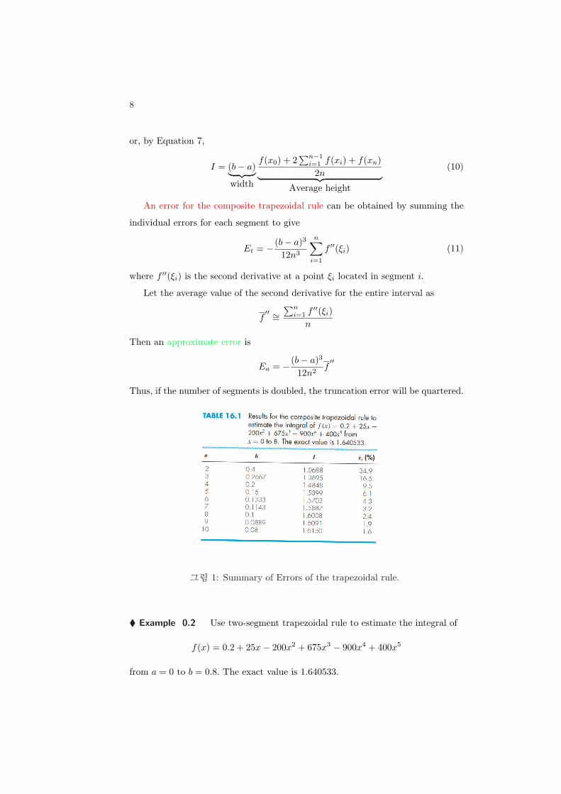
Thus, if the number of segments is doubled, the truncation error will be quartered.

ÕªaË> 1: Summary of Errors of the trapezoidal rule.

¨ Example 0.2 Use two-segment trapezoidal rule to estimate the integral of

f(x) = 0.2 + 25x− 200x2 + 675x3 − 900x4 + 400x5

from a = 0 to b = 0.8. The exact value is 1.640533.

9

Solution

For n = 2(h = 0.4):

f(0) = 0.2 f(0.4) = 2.456 f(0.8) = 0.232

I = 0.80.2 + 2(2.456) + 0.232

4= 1.0688

Et = 1.640533− 1.0688 = 0.57173 εt = 34.9%

Ea = − 0.83

12(2)2(−60) = 0.64

(12)

where −60 is the average second derivative determined previously.

MATLAB M-file : trap

A simple algorithm to implement the composite trapezoidal rule:

function I = trap(func, a, b, n)

% trap(func, a, b, n):

% composite trapezoidal rule.

% input :

% func = name of function to be integrated

% a, b = integration limits

% n = number of segments

% output :

% I = integral estimate

x = a;

h = (b-a)/n;

s = feval(func, a);

for j = 1 : n-1

x = x +h;

s = s + 2*feval(func, x);

end

s = s + feval(func,b);

I = (b-a)* s/(2*n);

10

¨ Example 0.3 By evaluating the integral of Equation 1, determine the dis-

tance fallen by the free-falling bungee jumper in the first 3 seconds. The exact

value of the integral is 41.94805.

Solution

g = 9.81m/s2, m = 68.1kg, and cd = 0.25kg/m

>> v = inline(’sqrt(9.81*68.1/0.25)*...

tanh(sqrt(9.81*0.25/68.1)*t)’)

v =

Inline function:

v(t) = sqrt(9.81*68.1/0.25)*...

tanh(sqrt(9.81*0.25/68.1)*t)

>> format long

>> trap(v,0,3,5)

ans =

41.86992959072735

>> trap(v,0,3,10000)

x =

41.94804999917528

SIMPSON’S RULESWe use higher-order polynomials such as a parabola(See Figure 16.11(a)) or a

third-order polynomial(See Figure 16.11(b)). The formulas that result from taking

the integral under these polynomials are called Simpson’s rules.

Simpson’s 1/3 Rule

Simpson’s 1/3 rule corresponds to the case where the polynomial in Equation 2

is second-order:

I =∫ x2

x0

[(x− x1)(x− x2)

(x0 − x1)(x0 − x2)f(x0) +

(x− x0)(x− x2)(x1 − x0)(x1 − x2)

f(x1)

+(x− x0)(x− x1)

(x2 − x0)(x2 − x1)f(x2)

]dx

(13)

where a and b are designated as x0 and x2, respectively. The result is

I =h

3[f(x0) + 4f(x1) + f(x2)] : Simpson’s 1/3 rule

11

or

I = (b− a)f(x0) + 4f(x1) + f(x2)

6(14)

where h = (b− a)/2.

Error(known)

Et = − 190

h5f (4)(ξ)

or, because h = (b− a)/2:

Et = − (b− a)5

2880f (4)(ξ) (15)

where ξ lies somewhere in the interval [a, b]. If a given polynomial is cubic, then

the error is 0. It yields exacts results for cubic polynomials even though it is

derived from a parabola!

¨ Example 0.4 Use Equation 14 to integrate

f(x) = 0.2 + 25x− 200x2 + 675x3 − 900x4 + 400x5

from a = 0 to b = 0.8. Employ Equation 15 to estimate the error. The exact

value is 1.640533.

Solution

For n = 2(h = 0.4):

f(0) = 0.2 f(0.4) = 2.456 f(0.8) = 0.232

12

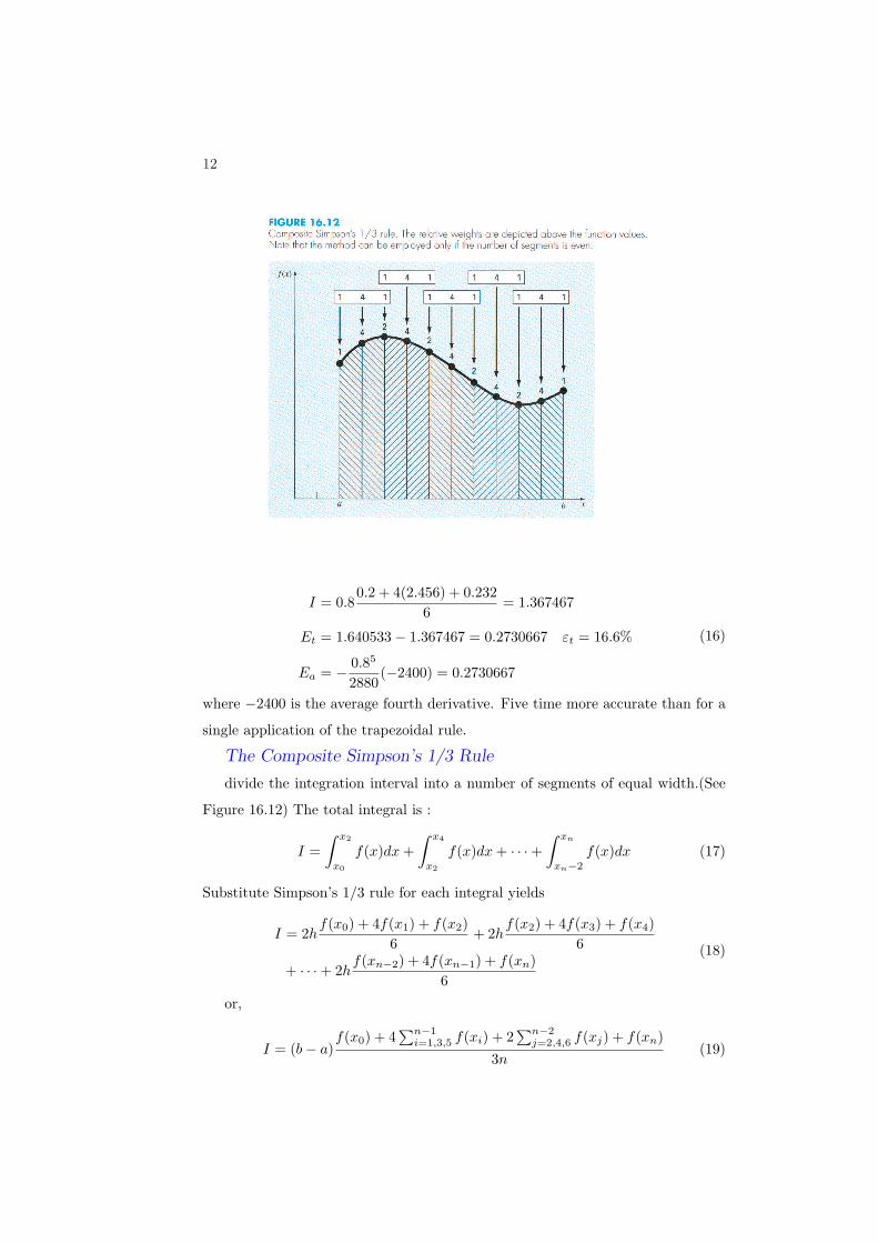
I = 0.80.2 + 4(2.456) + 0.232

6= 1.367467

Et = 1.640533− 1.367467 = 0.2730667 εt = 16.6%

Ea = − 0.85

2880(−2400) = 0.2730667

(16)

where −2400 is the average fourth derivative. Five time more accurate than for a

single application of the trapezoidal rule.

The Composite Simpson’s 1/3 Rule

divide the integration interval into a number of segments of equal width.(See

Figure 16.12) The total integral is :

I =∫ x2

x0

f(x)dx +∫ x4

x2

f(x)dx + · · ·+∫ xn

xn−2

f(x)dx (17)

Substitute Simpson’s 1/3 rule for each integral yields

I = 2hf(x0) + 4f(x1) + f(x2)

6+ 2h

f(x2) + 4f(x3) + f(x4)6

+ · · ·+ 2hf(xn−2) + 4f(xn−1) + f(xn)

6

(18)

or,

I = (b− a)f(x0) + 4

∑n−1i=1,3,5 f(xi) + 2

∑n−2j=2,4,6 f(xj) + f(xn)

3n(19)

13

where n is even(REQUIRED!!!).

An error estimate

Ea = − (b− a)5

180n4f

(4)(20)

¨ Example 0.5 Use Equation 19 with n = 4 to estimate the integral of

f(x) = 0.2 + 25x− 200x2 + 675x3 − 900x4 + 400x5

from a = 0 to b = 0.8. Employ Equation 20 to estimate the error. The exact

value is 1.640533.

Solution

For n = 4(h = 0.2):

f(0) = 0.2 f(0.2) = 1.288

f(0.4) = 2.456 f(0.6) = 3.464

f(0.8) = 0.232

I = 0.80.2 + 4(1.288 + 3.464) + 2(0.456) + 0.232

12= 1.623467

Et = 1.640533− 1.623467 = 0.017067 εt = 1.04%

Ea = − 0.85

180(4)4(−2400) = 0.017067

(21)

Note Et = Ea.

Restriction : even number of segments and equispaced. Then What? What?

What?

The Simpson’s 3/8 Rule

A third order Lagrange polynomial can be fit to four points and integrated to

yield

I =3h

8[f(x0) + 3f(x1) + 3f(x2) + f(x3)] : Simpson’s 3/8 rule

where h = (b − a)/3. It is the third Newton-Cotes closed integration formula.

Express it in the form of Equation 5:

I = (b− a)f(x0) + 3f(x1) + 3f(x2) + f(x3)

8(22)

An errors:

Et = − 380

h5f (4)(ξ)

14

or, because h = (b− a)/3:

Et = − (b− a)5

6480f (4)(ξ) (23)

Because the denominator of Equation 23 is larger than for Equation 15, the

3/8 rule is somewhat more accurate than the 1/3 rule.

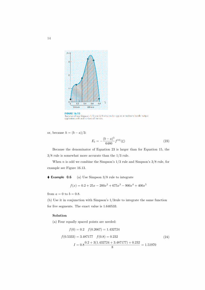
When n is odd we combine the Simpson’s 1/3 rule and Simpson’s 3/8 rule, for

example see Figure 16.13.

¨ Example 0.6 (a) Use Simpson 3/8 rule to integrate

f(x) = 0.2 + 25x− 200x2 + 675x3 − 900x4 + 400x5

from a = 0 to b = 0.8.

(b) Use it in conjunction with Simpson’s 1/3rule to integrate the same function

for five segments. The exact value is 1.640533.

Solution

(a) Four equally spaced points are needed:

f(0) = 0.2 f(0.2667) = 1.432724

f(0.5333) = 3.487177 f(0.8) = 0.232

I = 0.80.2 + 3(1.432724 + 3.487177) + 0.232

8= 1.51970

(24)

15

(b) five equally spaced points are needed(h = 0.16):

f(0) = 0.2 f(0.16) = 1.296929

f(0.32) = 1.743393 f(0.48) = 3.186015

f(0.64) = 3.181929 f(0.80) = 0.232

(25)

Simpson’s 1/3 rule for the first two segments

I1 = 0.320.2 + 4(1.296919) + 1.743393

6= 0.3803237

and for the last three segments, Simpson’s 3/8 rule used to obtain

I2 = 0.481.743393 + 3(3.186015 + 3.181929) + 0.232

8= 1.264754

So

I = I1 + I2 = 0.3803237 + 1.264754 = 1.645077

HIGHER-ORDER NEWTON-COTES FOR-MULAS

Newton-Cotes closed integration formulas : trapezoidal rule and Simpson’s

rule. Some of the formulas are summarized in Table 16.2. Simpson’s rules are

sufficient for most applications.

INTEGRATION WITH UNEQUAL SEGMENTS

Unequal-sized segments.

I = h1f(x0) + f(x1)

2+ h2

f(x1) + f(x2)2

+ · · ·+ hnf(xn−1) + f(xn)

2(26)

16

where hi = the width of segments i.

¨ Example 0.7 Trapezoidal Rule with Unequal Segments

The information in Table 16.3 was generated using the same polynomial em-

ployed in Example 0.1. Use Equation 26 to determine the integral for this data.

Recall that the correct answer is 1.640533.

Solution

I = 0.120.2 + 1.309729

2+ 0.10

1.309729 + 1.3052412

+ · · ·+ 0.102.363 + 0.232

2= 1.594801

(27)

with an absolute percent relative error of εt = 2.8%.

MATLAB M-file : trapuneq

A simple algorithm to implement the trapezoidal rule for unequally spaced

data can be written as below.

rules for x and y in the algorithm.

1. The two vectors are of the same length.

2. The x′s are in ascending order.

3. subscripts in Equation 26 need to be modified to account for the fact that

MATLAB does not allow zero subscripts in arrays.

The algorithm :

function integr = trapuneq(x, y)

% trapuneq(x,y):

% Applies the trapezoidal rule to determine

% the integral for n data points (x,y)

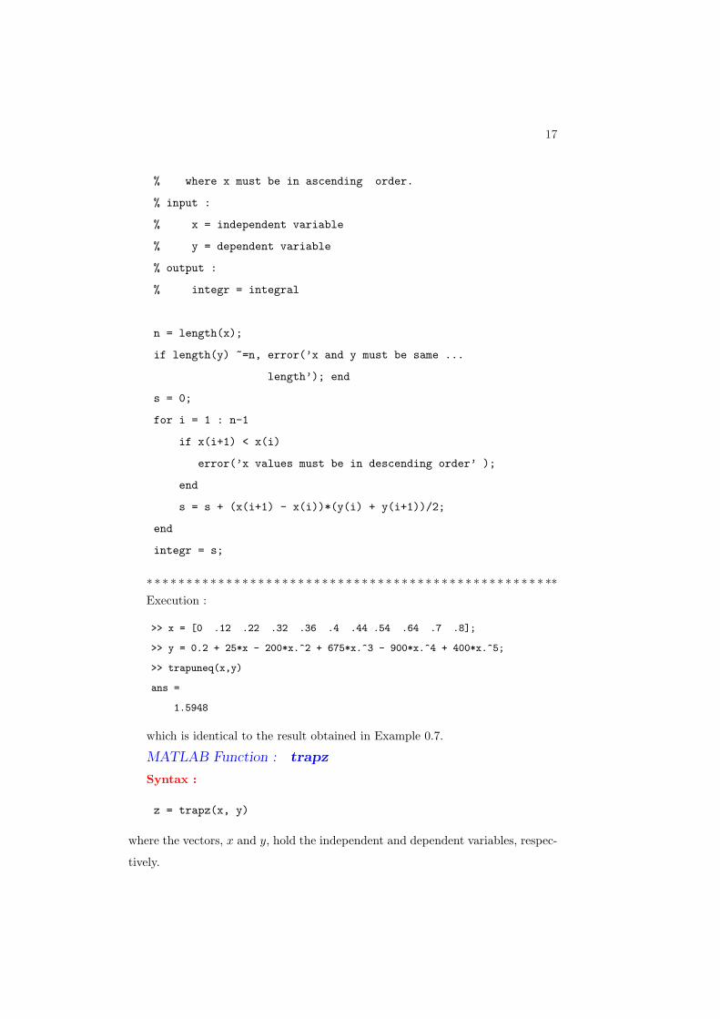
17

% where x must be in ascending order.

% input :

% x = independent variable

% y = dependent variable

% output :

% integr = integral

n = length(x);

if length(y) ~=n, error(’x and y must be same ...

length’); end

s = 0;

for i = 1 : n-1

if x(i+1) < x(i)

error(’x values must be in descending order’ );

end

s = s + (x(i+1) - x(i))*(y(i) + y(i+1))/2;

end

integr = s;

∗ ∗ ∗ ∗ ∗ ∗ ∗ ∗ ∗ ∗ ∗ ∗ ∗ ∗ ∗ ∗ ∗ ∗ ∗ ∗ ∗ ∗ ∗ ∗ ∗ ∗ ∗ ∗ ∗ ∗ ∗ ∗ ∗ ∗ ∗ ∗ ∗ ∗ ∗ ∗ ∗ ∗ ∗ ∗ ∗ ∗ ∗ ∗ ∗ ∗ ∗∗Execution :

>> x = [0 .12 .22 .32 .36 .4 .44 .54 .64 .7 .8];

>> y = 0.2 + 25*x - 200*x.^2 + 675*x.^3 - 900*x.^4 + 400*x.^5;

>> trapuneq(x,y)

ans =

1.5948

which is identical to the result obtained in Example 0.7.

MATLAB Function : trapz

Syntax :

z = trapz(x, y)

where the vectors, x and y, hold the independent and dependent variables, respec-

tively.

18

>> x = [0 .12 .22 .32 .36 .4 .44 .54 .64 .7 .8];

>> y = 0.2 + 25*x - 200*x.^2 + 675*x.^3 - 900*x.^4 + 400*x.^5;

>> trapz(x,y)

ans =

1.5948

OPEN METHODSRecall from Figure 16.6(b) that open integration formulas have limits that

extend beyond the range of the data. Table 16.4 summarize the Newton-Cotes

open integration formulas based on Equation 5 We will discuss it again in Chapter

18 and 19.

MULTIPLE INTEGRALSA general equation to compute the average of a two-dimensional function can

be written as

f =

∫ d

c(∫ b

af(x, y)dx)dy

(d− c)(b− a)(28)

The double integral of a function over a rectangular area(Figure 16.15)

¨ Example 0.8 Suppose that the temperature of a rectangular heated plate

is described by the following function :

T (x, y) = 2xy + 2x− x2 − 2y2 + 40

If the plate is 8 m long(x dimension) and 6 m wide(y dimension), compute the

average temperature.

19

Solution The correct answer is 58.66667. See Figure 16.16

The trapezoidal rule :

is implemented along x dimension for each y value. These value are then

integrated along the y dimension to give the final result of 2688. So 2688/(6×8) =

56.(How? HOMEWORK!!!!)

A single segment Simpson’s 1/3 rule :

2816/(6 × 8) = 58.66667. (How? HOMEWORK!!!!) We have exact value

because the given polynomial is quadratic. Note that Simpson’s 1/3 rule yielded

perfect results for cubic polynomial.