Embed Size (px)
Citation preview

Chapter 12: Indexing and HashingChapter 12: Indexing and Hashing

12.2
Chapter 12: Indexing and HashingChapter 12: Indexing and Hashing
Basic Concepts
Ordered Indices
B+-Tree Index Files
B-Tree Index Files
Static Hashing
Dynamic Hashing
Comparison of Ordered Indexing and Hashing
Index Definition in SQL
Multiple-Key Access

12.3
Basic ConceptsBasic Concepts
Indexing mechanisms used to speed up access to desired data.
E.g., author catalog in library
Search Key - attribute to set of attributes used to look up records in a file.
An index file consists of records (called index entries) of the form
Index files are typically much smaller than the original file
Two basic kinds of indices:
Ordered indices: search keys are stored in sorted order
Hash indices: search keys are distributed uniformly across “buckets” using a “hash function”.
search-key pointer

12.4
Index Evaluation MetricsIndex Evaluation Metrics
Access types supported efficiently. E.g.,
records with a specified value in the attribute
or records with an attribute value falling in a specified range of values.
Access time
Insertion time
Deletion time
Space overhead

12.5
Ordered IndicesOrdered Indices
In an ordered index, index entries are stored sorted on the search key value. E.g., author catalog in library.
Primary index: in a sequentially ordered file, the index whose search key specifies the sequential order of the file.
Also called clustering index
The search key of a primary index is usually but not necessarily the primary key.
Secondary index: an index whose search key specifies an order different from the sequential order of the file. Also called non-clustering index.
Index-sequential file: ordered sequential file with a primary index.

12.6
Dense Index FilesDense Index Files
Dense index — Index record appears for every search-key value in the file.

12.7
Sparse Index FilesSparse Index Files
Sparse Index: contains index records for only some search-key values.
Applicable when records are sequentially ordered on search-key
To locate a record with search-key value K we:
Find index record with largest search-key value < K
Search file sequentially starting at the record to which the index record points

12.8
Sparse Index Files (Cont.)Sparse Index Files (Cont.)
Compared to dense indices:
Less space and less maintenance overhead for insertions and deletions.
Generally slower than dense index for locating records.
Good tradeoff: sparse index with an index entry for every block in file, corresponding to least search-key value in the block.

12.9
Multilevel IndexMultilevel Index If primary index does not fit in memory, access becomes
expensive.
Solution: treat primary index kept on disk as a sequential file and construct a sparse index on it.
outer index – a sparse index of primary index
inner index – the primary index file
If even outer index is too large to fit in main memory, yet another level of index can be created, and so on.
Indices at all levels must be updated on insertion or deletion from the file.

12.10
Multilevel Index (Cont.)Multilevel Index (Cont.)

12.11
Index Update: DeletionIndex Update: Deletion
If deleted record was the only record in the file with its particular search-key value, the search-key is deleted from the index also.
Single-level index deletion:
Dense indices – deletion of search-key:similar to file record deletion.
Sparse indices –
if an entry for the search key exists in the index, it is deleted by replacing the entry in the index with the next search-key value in the file (in search-key order).
If the next search-key value already has an index entry, the entry is deleted instead of being replaced.

12.12
Index Update: InsertionIndex Update: Insertion
Single-level index insertion:
Perform a lookup using the search-key value appearing in the record to be inserted.
Dense indices – if the search-key value does not appear in the index, insert it.
Sparse indices – if index stores an entry for each block of the file, no change needs to be made to the index unless a new block is created.
If a new block is created, the first search-key value appearing in the new block is inserted into the index.
Multilevel insertion (as well as deletion) algorithms are simple extensions of the single-level algorithms

12.13
Secondary IndicesSecondary Indices
Frequently, one wants to find all the records whose values in a certain field (which is not the search-key of the primary index) satisfy some condition.
Example 1: In the account relation stored sequentially by account number, we may want to find all accounts in a particular branch
Example 2: as above, but where we want to find all accounts with a specified balance or range of balances
We can have a secondary index with an index record for each search-key value

12.14
Secondary Indices ExampleSecondary Indices Example
Index record points to a bucket that contains pointers to all the actual records with that particular search-key value.
Secondary indices have to be dense
Secondary index on balance field of account

12.15
Primary and Secondary IndicesPrimary and Secondary Indices
Indices offer substantial benefits when searching for records.
BUT: Updating indices imposes overhead on database modification --when a file is modified, every index on the file must be updated,
Sequential scan using primary index is efficient, but a sequential scan using a secondary index is expensive
Each record access may fetch a new block from disk
Block fetch requires about 5 to 10 micro seconds, versus about 100 nanoseconds for memory access

12.16
BB++-Tree Index Files-Tree Index Files
Disadvantage of indexed-sequential files performance degrades as file grows, since many overflow blocks
get created. Periodic reorganization of entire file is required.
Advantage of B+-tree index files: automatically reorganizes itself with small, local, changes, in the
face of insertions and deletions. Reorganization of entire file is not required to maintain
performance. (Minor) disadvantage of B+-trees:
extra insertion and deletion overhead, space overhead. Advantages of B+-trees outweigh disadvantages
B+-trees are used extensively
B+-tree indices are an alternative to indexed-sequential files.

12.17
Indexing StringsIndexing Strings
Variable length strings as keys
Variable fanout
Use space utilization as criterion for splitting, not number of pointers
Prefix compression
Key values at internal nodes can be prefixes of full key
Keep enough characters to distinguish entries in the subtrees separated by the key value
– E.g. “Silas” and “Silberschatz” can be separated by “Silb”
Keys in leaf node can be compressed by sharing common prefixes

12.18
Multiple-Key AccessMultiple-Key Access
Use multiple indices for certain types of queries. Example:
select account_number
from account
where branch_name = “Perryridge” and balance = 1000 Possible strategies for processing query using indices on single
attributes:
1. Use index on branch_name to find accounts with balances of $1000; test branch_name = “Perryridge”.
2. Use index on balance to find accounts with balances of $1000; test branch_name = “Perryridge”.
3. Use branch_name index to find pointers to all records pertaining to the Perryridge branch. Similarly use index on balance. Take intersection of both sets of pointers obtained.

12.19
Indices on Multiple KeysIndices on Multiple Keys
Composite search keys are search keys containing more than one attribute
E.g. (branch_name, balance)
Lexicographic ordering: (a1, a2) < (b1, b2) if either
a1 < b1, or
a1=b1 and a2 < b2

12.20
Indices on Multiple AttributesIndices on Multiple Attributes
With the where clause where branch_name = “Perryridge” and balance = 1000the index on (branch_name, balance) can be used to fetch only records that satisfy both conditions.
Using separate indices in less efficient — we may fetch many records (or pointers) that satisfy only one of the conditions.
Can also efficiently handle where branch_name = “Perryridge” and balance < 1000
But cannot efficiently handle where branch_name < “Perryridge” and balance = 1000
May fetch many records that satisfy the first but not the second condition
Suppose we have an index on combined search-key(branch_name, balance).

12.21
Non-Unique Search KeysNon-Unique Search Keys
Alternatives:
Buckets on separate block (bad idea)
List of tuple pointers with each key
Extra code to handle long lists
Deletion of a tuple can be expensive if there are many duplicates on search key (why?)
Low space overhead, no extra cost for queries
Make search key unique by adding a record-identifier
Extra storage overhead for keys
Simpler code for insertion/deletion
Widely used

12.22
Other Issues in IndexingOther Issues in Indexing
Covering indices Add extra attributes to index so (some) queries can avoid fetching
the actual records Particularly useful for secondary indices
– Why? Can store extra attributes only at leaf
Record relocation and secondary indices If a record moves, all secondary indices that store record pointers
have to be updated Node splits in B+-tree file organizations become very expensive Solution: use primary-index search key instead of record pointer in
secondary index Extra traversal of primary index to locate record
– Higher cost for queries, but node splits are cheap Add record-id if primary-index search key is non-unique

HashingHashing

12.24
Static HashingStatic Hashing
A bucket is a unit of storage containing one or more records (a bucket is typically a disk block).
In a hash file organization we obtain the bucket of a record directly from its search-key value using a hash function.
Hash function h is a function from the set of all search-key values K to the set of all bucket addresses B.
Hash function is used to locate records for access, insertion as well as deletion.
Records with different search-key values may be mapped to the same bucket; thus entire bucket has to be searched sequentially to locate a record.

12.25
Example of Hash File OrganizationExample of Hash File Organization
There are 10 buckets,
The binary representation of the ith character is assumed to be the integer i.
The hash function returns the sum of the binary representations of the characters modulo 10
E.g. h(Perryridge) = 5 h(Round Hill) = 3 h(Brighton) = 3
Hash file organization of account file, using branch_name as key (See figure in next slide.)

12.26
Example of Hash File Organization Example of Hash File Organization
Hash file organization of account file, using branch_name as key(see previous slide for details).
12.27
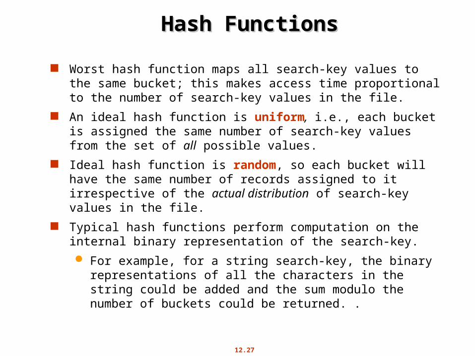
Hash FunctionsHash Functions
Worst hash function maps all search-key values to the same bucket; this makes access time proportional to the number of search-key values in the file.
An ideal hash function is uniform, i.e., each bucket is assigned the same number of search-key values from the set of all possible values.
Ideal hash function is random, so each bucket will have the same number of records assigned to it irrespective of the actual distribution of search-key values in the file.
Typical hash functions perform computation on the internal binary representation of the search-key.
For example, for a string search-key, the binary representations of all the characters in the string could be added and the sum modulo the number of buckets could be returned. .

12.28
Handling of Bucket OverflowsHandling of Bucket Overflows
Bucket overflow can occur because of
Insufficient buckets
Skew in distribution of records. This can occur due to two reasons:
multiple records have same search-key value
chosen hash function produces non-uniform distribution of key values
Although the probability of bucket overflow can be reduced, it cannot be eliminated; it is handled by using overflow buckets.
12.29
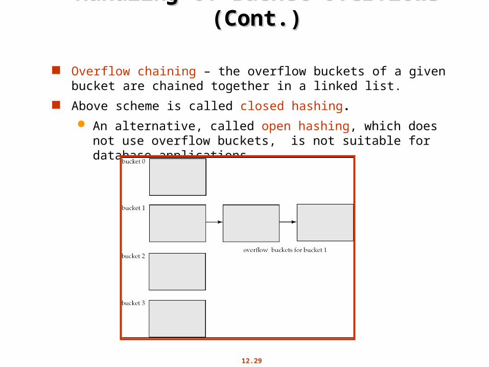
Handling of Bucket Overflows (Cont.)Handling of Bucket Overflows (Cont.)
Overflow chaining – the overflow buckets of a given bucket are chained together in a linked list.
Above scheme is called closed hashing.
An alternative, called open hashing, which does not use overflow buckets, is not suitable for database applications.

12.30
Hash IndicesHash Indices
Hashing can be used not only for file organization, but also for index-structure creation.
A hash index organizes the search keys, with their associated record pointers, into a hash file structure.
Strictly speaking, hash indices are always secondary indices
if the file itself is organized using hashing, a separate primary hash index on it using the same search-key is unnecessary.
However, we use the term hash index to refer to both secondary index structures and hash organized files.

12.31
Example of Hash IndexExample of Hash Index

12.32
Deficiencies of Static HashingDeficiencies of Static Hashing
In static hashing, function h maps search-key values to a fixed set of B of bucket addresses. Databases grow or shrink with time.
If initial number of buckets is too small, and file grows, performance will degrade due to too much overflows.
If space is allocated for anticipated growth, a significant amount of space will be wasted initially (and buckets will be underfull).
If database shrinks, again space will be wasted.
One solution: periodic re-organization of the file with a new hash function
Expensive, disrupts normal operations
Better solution: allow the number of buckets to be modified dynamically.

12.33
Dynamic HashingDynamic Hashing
Good for database that grows and shrinks in size Allows the hash function to be modified dynamically Extendable hashing – one form of dynamic hashing
Hash function generates values over a large range — typically b-bit integers, with b = 32.
At any time use only a prefix of the hash function to index into a table of bucket addresses.
Let the length of the prefix be i bits, 0 i 32.
Bucket address table size = 2i. Initially i = 0 Value of i grows and shrinks as the size of the database grows
and shrinks. Multiple entries in the bucket address table may point to a bucket
(why?)
Thus, actual number of buckets is < 2i
The number of buckets also changes dynamically due to coalescing and splitting of buckets.

12.34
General Extendable Hash Structure General Extendable Hash Structure
In this structure, i2 = i3 = i, whereas i1 = i – 1 (see next slide for details)

12.35
Use of Extendable Hash StructureUse of Extendable Hash Structure
Each bucket j stores a value ij All the entries that point to the same bucket have the same values on
the first ij bits.
To locate the bucket containing search-key Kj:
1. Compute h(Kj) = X
2. Use the first i high order bits of X as a displacement into bucket address table, and follow the pointer to appropriate bucket
To insert a record with search-key value Kj
follow same procedure as look-up and locate the bucket, say j.
If there is room in the bucket j insert record in the bucket.
Else the bucket must be split and insertion re-attempted (next slide.)
Overflow buckets used instead in some cases (will see shortly)

12.36
Deletion in Extendable Hash StructureDeletion in Extendable Hash Structure To delete a key value,
locate it in its bucket and remove it.
The bucket itself can be removed if it becomes empty (with appropriate updates to the bucket address table).
Coalescing of buckets can be done (can coalesce only with a “buddy” bucket having same value of ij and same ij –1 prefix, if it is
present)
Decreasing bucket address table size is also possible
Note: decreasing bucket address table size is an expensive operation and should be done only if number of buckets becomes much smaller than the size of the table
12.37
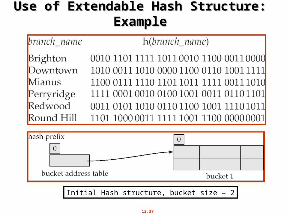
Use of Extendable Hash Structure: Use of Extendable Hash Structure: Example Example
Initial Hash structure, bucket size = 2

12.38
Example (Cont.)Example (Cont.)
Hash structure after insertion of one Brighton and two Downtown records

12.39
Example (Cont.)Example (Cont.)
Hash structure after insertion of Mianus record

12.40
Example (Cont.)Example (Cont.)
Hash structure after insertion of three Perryridge records

12.41
Example (Cont.)Example (Cont.)
Hash structure after insertion of Redwood and Round Hill records

12.42
Comparison of Ordered Indexing and HashingComparison of Ordered Indexing and Hashing
Cost of periodic re-organization
Relative frequency of insertions and deletions
Is it desirable to optimize average access time at the expense of worst-case access time?
Expected type of queries:
Hashing is generally better at retrieving records having a specified value of the key.
If range queries are common, ordered indices are to be preferred
In practice:
PostgreSQL supports hash indices, but discourages use due to poor performance
Oracle supports static hash organization, but not hash indices
SQLServer supports only B+-trees

12.43
Bitmap IndicesBitmap Indices
Bitmap indices are a special type of index designed for efficient querying on multiple keys
Records in a relation are assumed to be numbered sequentially from, say, 0
Given a number n it must be easy to retrieve record n
Particularly easy if records are of fixed size
Applicable on attributes that take on a relatively small number of distinct values
E.g. gender, country, state, …
E.g. income-level (income broken up into a small number of levels such as 0-9999, 10000-19999, 20000-50000, 50000- infinity)
A bitmap is simply an array of bits

12.44
Bitmap Indices (Cont.)Bitmap Indices (Cont.)
In its simplest form a bitmap index on an attribute has a bitmap for each value of the attribute
Bitmap has as many bits as records
In a bitmap for value v, the bit for a record is 1 if the record has the value v for the attribute, and is 0 otherwise

12.45
Efficient Implementation of Bitmap OperationsEfficient Implementation of Bitmap Operations
Bitmaps are packed into words; a single word and (a basic CPU instruction) computes and of 32 or 64 bits at once
E.g. 1-million-bit maps can be and-ed with just 31,250 instruction
Counting number of 1s can be done fast by a trick:
Use each byte to index into a precomputed array of 256 elements each storing the count of 1s in the binary representation
Can use pairs of bytes to speed up further at a higher memory cost
Add up the retrieved counts
Bitmaps can be used instead of Tuple-ID lists at leaf levels of B+-trees, for values that have a large number of matching records
Worthwhile if > 1/64 of the records have that value, assuming a tuple-id is 64 bits
Above technique merges benefits of bitmap and B+-tree indices

12.46
Index Definition in SQLIndex Definition in SQL
Create an index
create index <index-name> on <relation-name>(<attribute-list>)
E.g.: create index b-index on branch(branch_name)
Use create unique index to indirectly specify and enforce the condition that the search key is a candidate key is a candidate key.
Not really required if SQL unique integrity constraint is supported
To drop an index
drop index <index-name>
Most database systems allow specification of type of index, and clustering.

ExamplesExamples

12.48
Partitioned HashingPartitioned Hashing
Hash values are split into segments that depend on each attribute of the search-key.
(A1, A2, . . . , An) for n attribute search-key
Example: n = 2, for customer, search-key being (customer-street, customer-city)
search-key value hash value(Main, Harrison) 101 111(Main, Brooklyn) 101 001(Park, Palo Alto) 010 010(Spring, Brooklyn) 001 001(Alma, Palo Alto) 110 010
To answer equality query on single attribute, need to look up multiple buckets. Similar in effect to grid files.

12.49
Sequential File For Sequential File For account account RecordsRecords
12.50
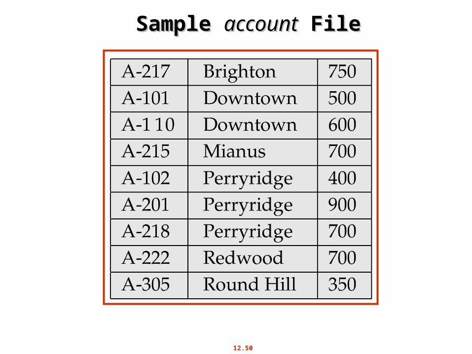
Sample Sample accountaccount File File

12.51
Figure 12.2Figure 12.2

12.52
Figure 12.14Figure 12.14

12.53
Figure 12.25Figure 12.25

12.54
Grid FilesGrid Files
Structure used to speed the processing of general multiple search-key queries involving one or more comparison operators.
The grid file has a single grid array and one linear scale for each search-key attribute. The grid array has number of dimensions equal to number of search-key attributes.
Multiple cells of grid array can point to same bucket
To find the bucket for a search-key value, locate the row and column of its cell using the linear scales and follow pointer

12.55
Example Grid File for Example Grid File for accountaccount

12.56
Queries on a Grid FileQueries on a Grid File
A grid file on two attributes A and B can handle queries of all following forms with reasonable efficiency
(a1 A a2)
(b1 B b2)
(a1 A a2 b1 B b2),.
E.g., to answer (a1 A a2 b1 B b2), use linear scales to find corresponding candidate grid array cells, and look up all the buckets pointed to from those cells.

12.57
Grid Files (Cont.)Grid Files (Cont.)
During insertion, if a bucket becomes full, new bucket can be created if more than one cell points to it.
Idea similar to extendable hashing, but on multiple dimensions
If only one cell points to it, either an overflow bucket must be created or the grid size must be increased
Linear scales must be chosen to uniformly distribute records across cells.
Otherwise there will be too many overflow buckets.
Periodic re-organization to increase grid size will help.
But reorganization can be very expensive.
Space overhead of grid array can be high.
R-trees (Chapter 23) are an alternative