CHAPTER 12 - dynamical-systems.org254 V. Badescu and R.B. Cathcart Of course, this limits the trajectory of the Sun to flight courses that may not be what human civilization most wants

CHAPTER 12

STELLAR ENGINES AND THE CONTROLLEDMOVEMENT OF THE SUN

VIOREL BADESCU1 AND RICHARD BROOK CATHCART2

1 Candida Oancea Institute, Polytechnic University of Bucharest, Spl. Independentei 313, Bucharest79590, Romania;2 Geographos, 1300 West Olive Avenue, Burbank, CA 91506, USA

Abstract: A stellar engine is defined in this chapter as a device that uses the resources of a star togenerate work. Stellar engines belong to class A and B when they use the impulse andthe energy of star’s radiation, respectively. Class C stellar engines are combinations oftypes A and B. Minimum and optimum radii were identified for class C stellar engines.When the Sun is considered, the optimum radius is around 450 millions km. Class A andC stellar engines provide almost the same thrust force. A simple dynamic model for solarmotion in the Galaxy is developed. It takes into account the (perturbation) thrust forceprovided by a stellar engine, which is superposed on the usual gravitational forces. Twodifferent Galaxy gravitational potential models were used to describe solar motion. Theresults obtained in both cases are in reasonably good agreement. Three simple strategiesof changing the solar trajectory are considered. For a single Sun revolution the maximumdeviation from the usual orbit is of the order of 35 to 40 pc. Thus, stellar engines of thekind envisaged here may be used to control to a certain extent the Sun movement in theGalaxy

Keywords: stellar engine, Kardashev type II civilization, Shkadov thruster, Dyson sphere, galaxygravitational potential, Sun movement control strategy

1. INTRODUCTION

For various reasons, mankind may be faced in the future with the problem ofchanging the Sun revolution motion. Avoiding nearby supernovae or ordinary starcollisions are examples. Diffuse matter clouds could also be a potential danger.Some studies suggest that during its lifetime the Sun has suffered about ten

251

V. Badescu et al. (eds.), Macro-Engineering: A Challenge for the Future, 251–279.© 2006 Springer.

252 V. Badescu and R.B. Cathcart

encounters with major molecular clouds (MMC) and it has had close (impact param-eter less than 20 pc) encounters with more than 60 MMC of various masses (Clubeand Napier, 1984; Napier, 1985). These events induce perturbations of the Oortcomet cloud, known to be sensitive to the particular galactic orbit of the Sun,leading to possible comet impacts on Earth (Gonzalez, 1999).

The Sun will steadily leave the main sequence in a few billion years, as stellarevolution calculations show (see e.g. Sackmann et al., 1993). The consequenceswill be a “moist greenhouse” effect on Earth, which will likely spell a definiteend to life on our planet well before the Sun will become a Red Giant (Kasting,1988; Nakajima et al., 1992). A preliminary solution to preserve the present-dayclimate on Earth may be to change its orbit. This subject is treated in detail inliterature (see, e.g. Korykansky et al., 2001; McInnes, 2002) and in Chapter 11 ofthis book.

Zuckerman (1985) estimates that if ancient extraterrestrial civilizations exist inthe Galaxy, then between 0.01 and 0.1 of them would have been forced to vacatetheir native planet due to the primary star leaving the main sequence. Problemswith feasibility and dynamics of mass interstellar migrations (Jones, 1981; Newmanand Sagan, 1981) prompted some researchers to propose the so-called “interstellartransfer” (or “solar exchange”) solution (Hills, 1984; Shkadov, 1987; Fogg, 1989).In this case the Earth (or, more generally, the home planet) is to be transformedinto a planet of a different star. The interstellar transfer requires first of all a wayof controlling Sun (or star) movement in the Galaxy.

In this chapter we study the amplitude of a possible human intervention on Sunrevolution motion. In section 2 we give a brief overview of different proposals inthe literature. Also, we define the concept of stellar engine and we give detailsabout various stellar engine classes. In section 3 we give the background physicsassociated to these devices. In section 4 we develop a model for the motion ofthe Sun in the Galaxy, based on usual Newtonian dynamics. The details of Sunmovement are complex but an “average” motion can be defined by using appropriateglobal Galaxy gravitational potentials. The movement is then studied in both thenormal (unperturbed) case and in the perturbed case, when an additional (stellarengine) thrust force is acting on the Sun. To increase the confidence in results, twodifferent global gravitational potentials are used. Finally, in the Conclusion sectionwe summarize the main findings of our work.

2. PROPOSALS TO CHANGE SUN MOTION

In his 12 May 1948 Halley Lecture at Oxford University in the UK, Fritz Zwicky(1889–1974) (see Zwicky, 1957) announced the possibility of

“! ! ! accelerating ! ! ! (the Sun) to higher speeds, for instance 1000 km/s directed toward Alpha CentauriA in whose neighborhood our descendents then might arrive a thousand years hence. [Such a one-waytrip] ! ! ! could be realized through the action of nuclear fusion jets, using the matter constituting the Sunand the planets as nuclear propellants”.

Stellar Engines 253

Zwicky’s Halley Lecture, which may be seen as a response to the 16 July 1945first nuclear fission explosion in the USA, was published in The Observatory(68:121–143, 1948) where the author merely hinted at the technical possibilities.At that time lasers were yet to be invented—circa 1960—and the controlled move-ment of asteroids and planets was still to be scientifically theorized (Korykansky,2004). However, during 1971 when SCIART, a blend of “Science” and “Art”,was organized by Bern Porter (1911–2004) even artists started to advocate use ofnuclear particle beams for peaceful projects. By 1992, the artist Francisco Infantevoiced his desire that humans redesign the firmament by intentionally shifting thepositions of the stars other than the Sun (Infante, 1992).

Thefirst scientifically recordedevidenceofanaturalcelestialbodyinspacecollidingwith the Sun came on 30-31 August 1979 when a cometary nucleus (1979 XI: Howard-Koomen-Michels) was observed as it vaporized in the Sun’s corona.

At the Conference on Interstellar Migration (held at Los Alamos, New Mexico, inMay 1983), David Russell Criswell extrapolated from available astronomical factsthat the Sun might never enter a Red Giant-stage because it will be transformedinto a stable White Dwarf-stage star via anthropogenic “star lifting”. Criswellspeculated about, perhaps proposed, a nameless macro-project the goal of whichwas to annually remove 6!5 ·1018 tons of solar plasma from the Sun for a period of∼300 million years—about 2% of the Milky Way Galaxy’s estimated age—settingaside the evicted plasma to cool by storing it near the Sun’s poles in a stable form.He foresaw this macro-engineering activity commencing circa AD 2170–5650.Criswell’s polar solar plasma lifts would be controlled and sustained versions ofthe Sun’s natural coronal mass ejections, which occur most everywhere on thatglowing celestial body’s turbulent surface. Criswell’s technique could be adaptedto spin-up the Sun, thus causing a mixing of its materials artificially. However,a too rapid equatorial rotation could force the Sun to become dangerously unstable.Criswell did not mention moving stars in his work. His stellar husbandry and starlifting concepts essentially involved mining stars in order to divide their mass intosmaller units so as to greatly extend their main sequence lifetime and the efficiencywith which their radiant energy could be utilised. It was Fogg (1989) who adaptedstar lifting to moving stars by accelerating mass from just one stellar pole ratherthan both.

Oliver Knill, in 1997, suggested deliberate triggering of asymmetric fusion andfission in the Sun might be utilized to move the Sun and its cortege of planets(Knill, 2003). He referred to solar flares, both natural and man-made, as “rockets onthe Sun”. He alleged that if all the Sun’s wind were focused in only one directioninstead of being emitted globally, then the Sun might, in principle, be acceleratedto a speed of 100 m/s in a year’s time. Since such total harnessing of the Sunis unlikely, Knill offered that giant solar flares might be induced which wouldhave the effect of propelling the Sun in a selected direction through space. Histechnical preference was to trigger huge artificial solar flares at one of the Sun’spoles that perform as rocket motors, lest the induced anthropogenic solar wind causeEarth serious problems of human health or civilization’s infrastructure breakdowns.


Of course, this limits the trajectory of the Sun to flight courses that may not bewhat human civilization most wants or needs. Like Fritz Zwicky, Knill opted forthe use of nuclear particle beams as a tool of rocket motor ignition.

Zwicky, Knill and Criswell, therefore, have proposed very advanced tele-miningmacro-projects that can have the planned effect of moving the Sun in some desireddirection (Fogg, 1989).

Another way of controlling the Sun’s movement is based on the concept of stellarengine. A stellar engine was defined in Badescu and Cathcart (2000) as a devicethat uses a significant part of a star’s resources to generate work. Three types ofstellar engines were identified and denoted as class A, B and C, respectively.

A class A stellar engine uses the impulse of the radiation emitted by a starto produce a thrust force. When acting through a finite distance the thrust forcegenerates work. As example of class A stellar engine we refer to the Sun thrusterproposed in Shkadov (1987), which consists of a mirror placed at some distancefrom the Sun (Fig. 1a). The mirror is situated such that the central symmetry of thesolar radiation in the combined mirror-Sun system is violated and, as a consequence,a certain thrust force will arise. For a mirror of given surface mass density a balanceexists between the gravitational force and the force due to solar radiation pressureat a certain mirror-Sun distance which remains constant. It may be shown that theequilibrium does not depend on the distance between mirror and the Sun, sinceboth the gravitational force and the force of the solar light pressure per unit mirrorsurface are inversely proportional to the square of the radius. A mirror with givengeometry located at 150 million km from the Sun requires a surface mass density ofabout 1!55 ·10−3 kg/m2 while its total mass amounts 1019 −1020 kg (which may becompared with the mass of the Earth, which is 5!977 ·1024 kg". Detailed calculationsmay be found in Shkadov (1987).

A class B stellar engine uses the energy flux of the radiation emitted by a starto generate mechanical power. An example of class B stellar engine was proposedin Badescu (1995). It consists of two concentric spherical “shells” centered on thestar. The “shells” have not necessarily continuous boundaries but they could be aswell as imaginary envelopes of a very large number of smaller 3D bodies englobingthe star. The inner surface acts as a solar energy collector. The outer surface is athermal radiator. The two surfaces have different but rather uniformly distributedtemperatures, Tp and Tr , respectively. The existing difference of temperature Tp −Tr

determines a heat flux from the inner towards the outer surface. This flux enteringthe thermal engine is used for power generation.

AclassCstellarenginewasdefined inBadescuandCathcart (2000)asacombinationof a class A and class B stellar engine (Fig. 1b). It uses the impulse and the energy ofthe star radiation to provide both a thrust force and mechanical power for its owningcivilization. Note that class B and C stellar engines are normally built by using thematerial of the inner planets (see Section 2.2). Of course, in this case the entire humanpopulation has to leave the Earth and move on the stellar engine.

For completeness here we define a new stellar engine as follows. A class D stellarengine uses a star’s mass to propel the star. A particular class D stellar engine is

Stellar Engines 255

Figure 1. (a). A class A stellar engine (Shkadov thruster). r – distance between star S and the mirror.! – mirror rim angle. (b). The class C stellar engine proposed in Badescu and Cathcart (2000).Rp – distance between star and inner surface, h – distance between inner and outer surfaces, TS – startemperature; Tp, Tr – temperatures of the inner and outer surfaces, respectively

the stellar rocket described in Fogg (1989), based on a modification of the conceptof “star lifting” proposed in Criswell (1985).

3. THERMODYNAMICS OF STELLAR ENGINES

3.1 Class A Stellar Engines

The energy radiated by a star is due to the nuclear reactions taking place in thenucleus. A steady-state star is characterized by a permanent balance between theenergy flux generated during the nuclear reactions and the energy flux emitted atstar’s surface in all directions.

The bolometric luminosity LS of the Sun (i.e. its energy radiated on all wave-lengths per unit time) is in present times (Ureche, 1987, p. 102):

(1) LS = 3"826 ·1026 W"

Let us consider the class A stellar engine of Fig. 1a. The star is prevented fromlosing energy on the solid angle covered by the mirror, as the energy emitted onthat direction is returned to the star together with the reflected radiation. As thenuclear reaction rate doesn’t change, the same energy flux LS has to be dissipated inspace but this time from the effective (not covered by the mirror) star surface only.Consequently, the photosphere temperature will increase and it is expected that thestar will change gradually to a different steady state. This effect was neglected inShkadov (1987).

One denotes by RS and TS the Sun’s ray and its present-day temperature, respec-tively. The area of the Sun surface (SS) and the surface of the Sun covered by themirror (SS#covered) are, respectively (Fig. 1a)

SS = 4$R2S(2)

SS#covered = 2$RSh(3)


Here h can be easily computed as a function of the mirror rim angle !

(4) h = RS"1− cos !#$

The effective (not covered by the mirror) Sun surface area, SS%eff , is:

(5) SS%eff = SS −SS%covered$

One supposes the Sun is a blackbody, both before and after mirror installation.Then the steady-state Sun temperature after mirror installation (TS) has to obey thefollowing energy balance equation:

(6) LS = SS&T 4S = SS%eff &T 4

S $

By using Eqs. (5) and (6) one obtains

(7) TS = TS!1−SS%covered/SS

"1/4 $

Using Eqs. (2)–(4) and Eq. (7) allows us to obtain the dependence of the Sun’stemperature TS on the mirror rim angle ! . Results are shown in Fig. 2. By increasingthe mirror’s rim angle the spectral class of the Sun gradually changes from G2towards F2 (Harvard classification).

The increase in the Sun’s photosphere temperature is accompanied by a changein its present absolute bolometric magnitude Mb. This change is governed by theequation (see Eq. (5.23) in Ureche, 1987, p. 109):

(8) Mb = Mb −10 lg#

TS

TS

$$

Figure 2. Dependence of Sun’s photosphere temperature Ts and absolute magnitude Mb on the mirror rimangle ! (see Fig. 1a). The relation between temperature and star spectral classes (Harvard classification)is also shown

Stellar Engines 257

Figure 2 shows the dependence of the absolute bolometric magnitude of the Sun,Mb, as a function of mirror rim angle ! . We have taken into account that the Sun’spresent absolute bolometric magnitude is Mb = 4"7.

One can see that for the rim angle considered by Shkadov (1987) in his calcu-lations (i.e. ! = 30!) both the photosphere temperature TS (and its associatedspectral class) and the absolute bolometric magnitude Mb remains quite close to thepresent-day values.

The mass of the mirror is distributed over a very large surface and, as a conse-quence, its influence on the orbit of the Earth is expected to be small. However,the Earth temperature may be affected in case of mirrors with large rim angle.Therefore, the mirror should be placed and kept in such a position that the orbit andtemperature of the Earth are not affected significantly (for example, the mirror-Sundirection may be kept perpendicular on Earth orbit).

3.2 The Dyson Sphere Revisited

In this section we shall consider a ‘usual’ thin Dyson sphere (DS) englobing theSun (Dyson, 1966). The inner DS surface constitutes the habitat of mankind. Dueto its symmetry, the Dyson sphere will have a rather uniform surface temperature.The DS material is assumed to have a good thermal conductivity. Consequently,one could neglect the thermal gradients on material’s thickness.

The steady-state energy balance per unit DS area is:

(9) aBS

#$T 4

S +a%1− BS

#&eint$T 4

p = %eint + eext&$T 4p "

Here a is the absorptance of DS inner surface while eint and eext is the emittanceof DS inner and outer surfaces, respectively. Also, TS and Tp is Sun and DStemperature, respectively. The first term in the l.h.s. of Eq. (9) is the energy fluxdensity absorbed from the Sun while the second term is the energy flux densityabsorbed from the whole Dyson sphere. The r.h.s. of Eq. (9) contains the energyflux densities emitted by the DS inner and outer surfaces, respectively.

The geometric factor BS in Eq. (9) may be computed as in Landsberg and Badescu(1998):

(10) BS ='!

0

cos ( sin (d(

2#!

0

d) = # sin2 '*

where ' is the half-angle of the cone subtended by the Sun when viewed from anarbitrary point placed on DS inner surface. One can simply prove that

(11) sin2 ' ="

RS

Rp

#2

*


where RS and Rp are Sun and DS radii, respectively. One denotes:

(12) x ≡ BS

!=!

RS

Rp

"2

"

The steady-state energy balance for the Sun’s surface is:

(13) 4!R2S#T 4

S −4!R2peint#T 4

p = LS"

The first term in the r.h.s. of Eq. (13) is the energy flux emitted by the whole surfaceof the Sun while the second term is the energy flux received by the whole surface ofthe Sun from the Dyson’s sphere. If one takes into account, on one hand, themultiple reflections of solar radiation on DS inner surface, and, on the other hand,the DS symmetry, one concludes that the absorptance a ≈ 1. This is only true if oneneglects that part of the radiation reflected by DS inner surface which is incident onthe Sun’s surface. By solving the Eqs. (9) and (13) and taking into account Eq. (12)one obtains:

Tp =#

LS

4!R2p#eext

$1/4

(14)

TS =%!

1+xeint

eext

"LS

4!R2S#

&1/4

"(15)

These relations are valid under the condition TS > Tp, which may be re-written (byusing Eqs. 12, 14 and 15) as:

(16) Rp ≥!

1− eint

eext

"1/2

RS"

Figure 3 of Badescu and Cathcart (2000) shows the dependence of DS temperatureTp on the radius for various values of DS surface emittance e = eint = eext.A surface temperature comparable with present-day average ground surface temper-ature (∼300 K) corresponds to high values of surface emittance. A number ofconclusions may be drawn. First, small radii increase the feasibility of a DS projectas the amount of material required is proportional to R2

p. Second, the inner planetsseem to be the best source of material in this case due to the shorter distance betweentheir orbit and the place of the future Dyson sphere. The material of the inner planetshas a relatively low albedo (between 0.07 in case of Mercury and 0.39 in Earth case(Moore, 1970); Venus’ high albedo is due to its cloudy atmosphere). Normally, lowalbedo values are associated to surfaces with high absorptance (or, which equiva-lent due to Kirchoff’s law, to surfaces with high emittance). Therefore, the innerplanets are appropriate for DS building also from the point of view of their opticalproperties.

Stellar Engines 259

3.3 Class B and Class C Stellar Engines

Due to mirror’s imperfect reflection and to the finite size of the Sun, a spot ofconcentrated light is expected to appear on the inner surface of class B and class Cstellar engines in its part opposite to the mirror. This spot is associated with atemperature peak and can be used to increase locally the work rate provided bythe thermal engine. However, for convenience we shall assume: (i) the Sun has anegligible size as compared to the radius of the stellar engine and (ii) the mirror isperfect (i.e. the mirror has a unity reflectance and it reflects all the incident rays onSun’s direction). As a consequence, the mirror temperature is very low and is notconsidered in this work.

Now, we shall analyze a region on the inner surface of the class B stellar engine(or on that part of the class C stellar engine that is used for power generation). Thesteady-state energy balance per unit area of the inner surface is:

(17) qH = BS

!" T 4

S +!

1− BS

!

"eint" T 4

p − eint" T 4p #

Here, qH is the energy density flux entering the thermal engine (Fig. 3). The firstand the second terms in the r.h.s of Eq. (17) is the energy flux density absorbedfrom the Sun and from the whole stellar engine inner surface, respectively. Here,the conservation of the etendue on the mirror surface is taken into account (see e.g.Badescu, 1993, and references therein). The third term in the r.h.s of Eq. (17) isthe energy flux density emitted by the stellar engine’s inner surface.

The energy balance per unit area of the outer surface is:

(18) qL = eext" T 4r #

In Eq. (18) qL is the energy flux density leaving the thermal engine per unit surfacearea while Tr is the temperature of the outer surface of the stellar engine.

Here a particular case of endoreversible thermal engine is considered, namely theChambadal-Novikov-Curzon-Ahlborn engine (CNCA engine for short). It consistsof three parts (Fig. 3):

(a) a reversible part working between two heat reservoirs (one at the high temper-ature), say t1, and one at the low temperature, say t2; (usually, t1 and t2 are thetemperatures of the working fluid during its isothermal expansion and compression,respectively).

(b) two irreversible parts containing temperature drops (i.e. the temperature fallTp − t1 accompanying qH and the temperature fall t2 −Tr accompanying qL). A linearrelationship exists between the heat flows and the temperature gradients.

Details on endoreversible and CNCA engines may be found in the reviews byBejan (1996) and Hoffmann et al., (1997).

The entropy balance for the CNCA engine is (De Vos, 1985):

(19)qH

T 1/2p

+ qL

T 1/2r

= 0#


Figure 3. Power generation by using a CNCA thermal engine. qH! qL – heat fluxes entering and leavingthe thermal engine, respectively; t1 and t2 – the absolute temperatures of the working fluid in contactwith the two heat reservoirs. Tp! Tr – temperatures of the inner and outer surfaces, respectively; w –work rate (power)

The energy balance for the whole surface of the Sun is:

(20) SS!eff "T 4S −SSeint"T 4

p = LS#

The first term in the l.h.s. of Eq. (20) is the energy flux lost by the Sun; it takesinto consideration that all the energy emitted by the Sun on mirror’s direction isreflected back. The second term in the l.h.s. of Eq. (20) is the energy flux receivedby the Sun from the inner surface of the stellar engine. It takes into account that,due to the perfect mirror, each unit surface area of the Sun receives the energy fluxdensity eint"T 4

p .Simple computation shows that:

(21) SS!eff = SS

1+ cos $

2#

One uses the following notation:

(22) %S ≡ TS

TS

%p ≡ Tp

TS

%r ≡ Tr

TS

#

In the following %p is supposed to be known. This is a reasonable assumption asnormally Tp should allow living conditions and consequently has a small variationrange. By using Eqs. (12) and (17)–(22) one derives:

%S =!

eint%4p + 2

1+ cos $

"1/4

(23)

%r =#

21+ cos $

x

eext

1

%1/2p

$1/4

#(24)

Stellar Engines 261

The two following conditions have to be fulfilled: !S > !p and !p > !r , in orderfor the thermal engine to operate (i.e. to generate a positive power). By usingEqs. (22)–(24) these conditions turn out to be:

eint ≥ 1− 2!4

p "1+ cos #$(25)

Rp ≥ RS

!2

eext!4p "1+ cos #$

"1/2

%(26)

The constraint Eq. (25) is always fulfilled as its r.h.s. member is non-negative,because !p < 1 (see Eq. 22) and cos # ≤ 1. On the other hand, Eq. (26) gives aminimum limit for the radius of the stellar engine.

Let us have a look to the class B stellar engine proposed in Badescu (1995).It may be seen as a particular case of class C stellar engine (it corresponds toa missing mirror or, in other words, to # = 0$$. For an outer surface emittanceeext = 1 one finds the minimum radius Rp&min = RS/!2

p. This is very close to the resultRp&min = RS"1 − !4

p$1/2/!2

p derived in Badescu (1995) without taking into accountthat the presence of the stellar engine increases the Sun’s temperature.

Figure 5 of Badescu and Cathcart (2000) shows the dependence of the Suntemperature TS on the mirror rim angle # and the radius Rp of the stellar engine.Generally, TS increases with increasing # and the radius Rp. However, this appliesmainly for Rs < 400 ·106 km.

Figure 4a shows the dependence of the outer surface temperature Tr on # and Rp.Generally, Tr decreases by increasing Rp and decreasing the mirror rim angle # .

Knowledge of the temperature Tr is important in case of searching for extraterres-trial intelligence (SETI). Indeed, it is (practically) the only information that outsideworld receives from a Kardashev type II civilisation. One reminds that according tothe classification proposed by Kardashev a technological civilisation is of type I, IIor III if it has under its control the materials and energy resources of a planet, star,or galaxy, respectively (see Kardashev, 1964; Badescu and Cathcart, 2000). FromFig. 4a one learns that galactic IR sources corresponding to temperatures lowerthan 300 K should not be overlooked during SETI activities. For more informationabout the thermal signature of possible extraterrestrial civilizations in the Galacticcontext see Chapter 13 in this book.

The heat flux density qH is obtained by using Eqs. (12), (17), (22)–(24):

(27) qH = x'T 4S

21+ cos #

%

The well-known CNCA efficiency is (De Vos, 1985)

(28) (CNCA = 1−#

Tr

Tp

$1/2

= 1−#

!r

!p

$1/2

%


Figure 4. Dependence of various quantities on mirror rim angle ! and radius Rp in case of a class Cstellar engine. (a) Outer surface temperature Tr (K); (b) Thermal engine efficiency "CNCA; (c). Powerdensity wCNCA #W/m2$; (d) Optimum inner surface temperature Tp (K). In cases (a), (b), (c) thetemperature of the inner surface is Tp = 300 K and the emittance of both inner and outer surfaces iseint = eext = 0%8. In case (d) eint = eext = 1

Figure 4b show the dependence of &CNCA on ! and Rp. This performance indicatorincreases by increasing the radius Rp and decreasing the mirror rim angle ! . Onecan see that the efficiency vanishes and tends to become negative for Rp valuessmaller than the limit predicted by Eq. (26) (see the top left corner of Fig. 4b,where the associated “critical” rim angle may be easily evaluated). Generally,&CNCA is smaller than the efficiency (which may exceed 0.5) of common terrestrialpower plants working at large temperature differences but it is comparable with theefficiency of Stirling engines working at small differences of temperature (tens ofKelvin)(see Badescu, 2004).

Figure 8 of Badescu and Cathcart (2000) shows the dependence of &CNCA on theouter surface emittance eext. The efficiency increases by increasing eext. This canbe explained as follows. Increasing the emittance eext makes the temperature Tr

decrease (see Fig. 5) and this finally leads to an increase in the efficiency. This has

Stellar Engines 263

Figure 5. Dependence of the power density wCNCA and of the outer surface temperature Tr on the outersurface emittance eext in case of a class C stellar engine. Rp = 300 millions km and ! = 30 degrees.Other inputs as in Fig. 4a

again consequences for SETI activities. Indeed, the thermal signature of possibleextraterrestrial civilizations may be at a lower level than commonly expected.

The work rate (power) density wCNCA is given by:

(29) wCNCA = qH"CNCA#

Figure 4c shows that for small Rp values the power density wCNCA decreases byincreasing the mirror rim angle ! . However, at high Rp values the reverse happens.There is a maximum maximorum power density which corresponds in both casesto a Rp radius of about 450 · 106 km. This means that there is an optimum stellarengine radius. That optimum radius is obviously larger than the radius of commonlyproposed Dyson spheres, which is of the order or Earth orbit radius. One can noticethat for some values of Rp and ! the power density wCNCA becomes negative (lefttop corner of Fig. 4c).

Figure 5 shows the dependence of the power density wCNCA and of the temperatureTr on the emittance of the outer surface eext. As expected, the temperature Tr

decreases by increasing eext. But decreasing Tr leads to an increase in the efficiency(see Fig. 8 of Badescu and Cathcart, 2000) and finally this is associated with anincrease in the power density wCNCA.

Practically, wCNCA and Tr do not depend on the emittance of the inner surface eint.

3.4 The Thrust Force Acting on the Sun

We showed in Section 3.1 that the presence of the mirror makes the Sun’s temper-ature increase. This has consequences on the radiation impulse and finally on thethrust force acting on the Sun. In this section one evaluates the thrust force in caseof both class A (Shkadov thruster) and class C stellar engines.


3.4.1 Class A stellar engine (Shkadov thruster)

The impulse of the radiation per unit time leaving the Sun is proportional to theenergy emitted (see Shkadov, 1987):

(30) p = SS!T 4S

c"

By taking into account the Eqs. (5)–(7), (21) and (30) one obtains:

(31) p = LS

c

21+ cos #

"

Note that in Shkadov (1987) the increase in Sun temperature due to mirror’sexistence is not considered and the following approximate relation is used: p = LS/c.

The thrust force f per unit area in the direction of the normal n to an arbitraryunit area placed on the base surface of the spherical cone A’SB’ of Fig. 1a is (seealso Fig. 1 of Shkadov, 1987):

(32) f = LS

c

21+ cos #

14$R2

p

"

When # = 0, Eq. (32) reduces to Eq. (1) of Shkadov (1987). The correction factor2/ %1+ cos #& takes into account the increase in Sun’s temperature.

The thrust F being produced by the Sun-mirror system due to the non-symmetricradiation field is given by Shkadov (1987)

(33) F =!

f · n' dS(

where S is the base area of the spherical cone A’SB’ in Fig. 1a while ' is the unitvector along the axis of that cone. After integration one obtains:

(34) F = LS

2c%1− cos #&"

When # = 0, Eq. (34) reduces to Eq. (2) of Shkadov (1987). The thrust force Fincreases by increasing the mirror rim angle # , as expected. The original resultis 4cF = LS sin2 # (see Eq. 2 of Shkadov, 1987). One can see that our Eq. (34)generally estimates a higher thrust force, which, in the particular case # = 90",doubles the result obtained by using Eq. (2) of Shkadov (1987). The main conse-quence is the fact that the lateral deviation during one orbital period of the Sun,evaluated by Shkadov (1987) to about 4.4 parsec, is underestimated. The valueestimated by Shkadov (1987) for the acceleration induced by the thrust force F onthe solar system motion is 6"5 · 10−13 m/s2. This is half of the result obtained byusing the improved model from this chapter. Both values have to be compared withthe gravitational acceleration of the galactic field, which is about 1"85 ·10−10 m/s2

(Shkadov, 1987). One concludes that the magnitude of the disturbing force createdby the sun-mirror system is small, as expected.

Stellar Engines 265

3.4.2 Class C stellar engine

The impulse of the radiation emitted by the inner surface of a class C stellar engineat temperature Tp impinging on the Sun, in case that no mirror exists, is:

(35) pD =4!R2

Seint"T 4p

c#

By using the notations Eqs. (22) and Eqs. (23)-(24) one obtains:

(36) pD = LS

ceint

$4p

$4S

#

Consequently, the impulse of the net flux of radiation leaving the Sun is:

(37) pnet = p−pD#

By taking into account the Eqs. (35)–(37) one obtains:

(38) pnet = LS

c

!

1− eint

$4p

$4S

"2

1+ cos %#

The thrust force f per unit area in the direction of the normal n to the basesurface of the circular cone A’SB’ (see Fig 1a) is:

(39) f = LS

c

!

1− eint

$4p

$4S

"2

1+ cos %

14!R2

p

#

The thrust force F is obtained after computing the integral in Eq. (33):

(40) F = LS

2c

!

1− eint

$4p

$4S

"

&1− cos %'#

Generally, the thrust force F increases by increasing the mirror rim angle % . Onehas to remind, however, that increasing % leads to a decrease in the efficiency (CNCA

(see Fig. 4b). Note that F is dependent on the temperature Tp via the dimensionlessparameter $p. The optimum value of TP which maximizes F is shown in Fig. 4d foreint = eext = 1. Let us consider an optimum temperature Tp∼300 K (appropriate forcommon living conditions on Earth). Then F is a maximum for a radius Rp around300 millions km.

In the next sections one shall need the thrust force F ′ per unit mass of the solarsystem. This implies dividing the Eqs. (34) and (40), respectively, by MS +Mplanets,where MS = 1#989 · 1030 kg and Mplanets = 2#7 · 1027 kg are Sun mass and the mass


of Solar System’s planets, respectively. Then, the expressions of F ′ for class A andclass C stellar engines are, respectively:

F ′A = LS

2c

1− cos !

MS +Mplanets

(41)

F ′C = LS

2c

!

1− eint

"4p

"4S

"1− cos !

MS +Mplanets

#(42)

When used in case of the Sun, the Eqs. (41) and (42) lead to (practically) thesame numerical results. This is due to the fact that eint$"p/"S% ∝ $300/5760%4 isvery close to zero. Consequently, the results reported below apply to both types ofstellar engines and the indexes A or C will be removed for convenience.

4. CHANGE OF SUN MOVEMENT IN GALAXY

The Sun’s galactic orbit is described here by ignoring the perturbations due toGalaxy spiral arms and the encounters with massive dust/molecular clouds. Thegravitational forces acting on the Sun in the absence of a stellar engine aremodeled as being derived from scalar potentials. Various gravitational potentialswere proposed and studied in the relevant literature. It is not our aim to decidewhich of these potentials is more appropriate to be used in practice. Here we shalluse the simple spherical potential adopted earlier by Shkadov (1987) (see section4.1 below). However, some authors consider it to be helpful to decompose the Sun’smotion into two orthogonal components: a motion in the galactic mid-plane and amotion perpendicular to the plane (Gonzalez, 1999). Therefore, a cylindrical grav-itational potential will be used in Section 4.2. It is a generalization of a Plummerpotential, previously used by Carlberg and Innanen (1987). We shall see that bothpotentials predict results of the same order of magnitude and this may act as a sortof cross-checking.

The stellar engine thrust force F is superposed on the Galaxy gravitational forcesacting on the Sun. As a result, a perturbed Sun trajectory will result. It is the scopeof the present section to evaluate the distance between the perturbed position andthe Sun’s usual (average) position.

4.1 Movement in Curvilinear Coordinates

A few results of vector analysis are used here to describe Sun motion. We definea cartesian system of coordinates

#xi$

$i = 1& 2& 3% with the plane Ox1x2 in theequatorial plane of the Galaxy. The Sun movement in the Galaxy will be given bythree parametric functions, say xi = xi $t% $i = 1& 2& 3%. A curvilinear coordinationsystem qi $i = 1& 2& 3% is then introduced. The transformation

#xi$

→#qi$

defines ametric tensor gij $i& j = 1& 2& 3%. One denotes by qi the usual first order time deriva-tives of the coordinates qi $i = 1& 2& 3%. They are called generalized velocities. Note

Stellar Engines 267

that their dimensions are not necessarily length per time. The connection betweenqi and the components of Sun’s velocity vi (i.e. the projections on the coordinatesqi !i = 1" 2" 3## are given by the usual relationships (Beju et al., 1976, p 173):

(43) vi = Hiqi !i = 1" 2" 3# "

where Hi are the Lamé coefficients, which can be obtained by (Beju et al., 1976, p 172):

(44) Hi = g1/2ii !i = 1" 2" 3# $

The contravariant time derivative D/Dt of the generalized velocities qi is givenby (Beju et al., 1976, p 183)

(45)Dqi

Dt= dqi

dt+% i

jkqj qk"

where % ijk are Christoffel coefficients of the second kind. Here the Einstein conven-

tion for summation was used. The equations of movement of the Sun have thecovariant form:

(46) ai = Hi

Dqi

Dt= Gi +F

′i !i = 1" 2" 3# "

where ai is the i-th contravariant component of Sun’s acceleration while Gi and F′i

are the i-th contravariant components of the gravitational force and of the stellarengine thrust, respectively, both of them per unit mass of the Solar System.

The Sun motion is described first by mean of the spherical coordinate system!R"&"'# used in Shkadov (1987). The change of coordinates

!x1"x2"x3

"→

!R"&"'# is:

(47) x1 = R cos ' cos & x2 = R cos ' sin & x3 = R sin '"

where 0 ≤ & ≤ 2( and −(/2 ≤ ' ≤ (/2. The equatorial plane of the Galaxy isassociated to ' = 0. Details about the metric tensor gij, the contravariant tensorgij !i" j = R"&"'#, the Lamé coefficients and the Christoffel symbols of first andsecond kind, respectively, may be found in Badescu and Cathcart (2006).

Use of Eqs. (43) allows to obtain the components vi !i = R"&"'# of Sun’s velocity:

(48) vR = R v& = R cos '& v' = R'"

while use of Eqs. (44)–(46) and (48) allow to obtain the components vi !R"&"'#of Sun’s acceleration:

(49)

vR =!v&"2 + !v'#2

R+GR +F

′R

v& = −vRv& −v&v' tan '

R+G& +F

′&

v' = −v&v' +!v&"2

tan '

R+G' +F

′'

$


The Sun motion is described now by mean of the cylindrical coordinate system!r" #" z$ used in Carlberg and Innanen (1987). The change of coordinates!x1"x2"x3

"→ !r" #" z$ is:

(50) x1 = r cos # x2 = r sin # x3 = z"

where 0 ≤ # ≤ 2%. The equatorial plane of the Galaxy is associated to z = 0. Again,details about the metric tensor gij, the contravariant tensor gij !i" j = r" #" z$, theLamé coefficients and the Christoffel symbols of first and second kind, respectively,may be found in Badescu and Cathcart (2006).

Use of Eqs. (43) allows to obtain the components vi !i = r" #" z$ of Sun’s velocity:

(51) vr = r v# = r# vz = z"

while use of Eqs. (44)–(46) and (51) allow to obtain the components vi !r" #" z$ ofSun’s acceleration:

(52)vr =

!v#"2

r+Gr +F

′r

v# = −vrv#

r+G# +F

′#

vz = Gz +F′z

&

The above theory will be used now in case of two Galaxy gravitational potentials.

4.2 First Galaxy Gravitational Potential

As a first axi-symmetrical gravitational potential per unit mass of the solar system,' !R"(")$, we shall adopt:

(53) ' !R"(")$ = A

B+ !B2 +R2$1/2 − C2 tan2 !)/2$

R2 !1+D2 tan2 !)/2$$1/2 &

Here a spherical system of coordinates !R"(")$ was used. The constants in Eq. (53)are as follows: A = 3&18 ·1022 km3/s2, B = 8&6 ·1016 km, C = 3&27 ·1020 km2/s andD = 30&8 (Shkadov, 1987).

The components of the gradient of ' are projections of the gravitational accel-eration vector G:

(54) GR = 1HR

*'

*RG( = 1

H(

*'

*(= 0 G) = 1

H)

*'

*)&

Here the Lamé coefficients Hi !i = R"(")$ were used.One denotes the components of Sun’s velocity by vi !i = R"(")$ and one defines

the following dimensionless variables:

(55) t ≡ t

T0R ≡ R

r0vR ≡ vR

v0v( ≡ v(

v0v) ≡ v)

v0"

Stellar Engines 269

where T0

!= 220 ·106 yr

", r0 != 8500 pc" and v0 != 12 km/s" are appropriate

scaling values.In the dimensionless notation Eq. (55), the Eqs.(48) and (49) describing the Sun

movement are:

(56a-e)

˙R= vR # = v#

R cos $# = v#

R cos $

˙vR = D1

!v#"2 + !v$"2

R− D2a

R!B2 + R2

"1/2#B2 +

!B2 + R2

"1/2$2

+D2b

2 tan2 !$/2"

R3!1+D2 tan2 !$/2""1/2

+fRD3

v# =−D1vRv# − v#v$ tan $

R+f #D3

˙v$ =−D1

v#v$ +!v#"2

tan $

R

−D2b

1+ D2

2 tan2 !$/2"

R3 !1+D2 tan2 !$/2""1/2

tan2 !$/2"

cos2 !$/2"+f$D3%

Here the Eqs. (42) and (30) and the dimensionless parameters defined below werealso used:

(57)B ≡ B

r0D1 ≡ v0T0

r0D2a ≡ T0A

v0r20

D2b ≡ T0C2

v0r30

D3 ≡ T0

v0

Ls

2c

1− cos &

Msun +Mplanets

!1− eint'4

p

'4s"

%

In Eqs. (56) the unit vector!fR(f #(f$

"gives the direction of the thrust force per

unit mass F ′ (see Eq. 42) in the coordinate system !R(#($".A simplifying hypothesis was adopted in Shkadov (1987) to allow an analytical

solution for the perturbed motion of the Sun. Thus, one considered a particularset of initial conditions that makes the usual (unperturbed) motion of the Sun tobe along a circular orbit in the equatorial plane $ = 0 of the Galaxy. One provedthat the ratio of the maximum acceleration generated by the Sun-mirror systemto the Galaxy gravitational acceleration is less than one percent. One concludedthat the magnitude of the thrust force is (relatively) small and the small parametermethod can be used to solve the equations of the perturbed motion. Consequently,the perturbed motion of the Sun was described mathematically in Shkadov (1987)as a variational problem with respect to the unperturbed (circular) orbit.


In this chapter the Eqs. (56) are solved numerically by using the ODE-solverSDRIV3 from the SLATEC library (Fong et al., 1993).

A few details about the initial values used to solve the Eqs. (56) follow. The(absolute) Sun velocity is usually obtained by adding the (average) near circularvelocity of the Galaxy at the Sun to the Sun’s velocity in the local standard of rest(LSR). Discussions on various ways of defining the LSR can be found in (Bash,1986, p. 42). One knows that the Sun is located near the corotation circle, wherein a spiral galaxy such as ours the angular speeds of the spiral pattern and thestars are equal (Mishunov and Zenina, 1999). Consequently, one expects a rathersmall value for Sun’s velocity in the LSR. Indeed, HIPPARCOS-based studies givethe mean value 13!4 ± 0!4 km/s (Dehnen and Binney, 1998; Kovalevsky, 1999;Bienayme, 1999). The LSR velocity is higher for older than for younger stars dueto accumulation of perturbations to a star’s trajectory. Consequently, the present-day orbit differs from the originally nearly circular motion in plane (Gonzalez,1999). One defines the Sun’s velocity components "u#v#w$ in the LSR as follow:u is the velocity positive outward away from the galactic center; v is the velocityin the galactic plane positive in the sense of the galactic rotation and w is thevelocity in the direction perpendicular on the galactic plane, positive toward thenorth galactic pole (Bash, 1986, p. 36). In this convention "u#v#w$ = "0# 0# 0$characterizes a body at Sun position, moving in the galactic plane on a circularorbit. The initial components of LSR Sun velocity are denoted "u0#v0#w0$. Incomputation we used the rather popular values (in km/s):"u0#v0#w0$ = "−9# 12# 7$(Bash, 1986, p. 36; Darling, 2004). The local components "U#V#W $ of Galaxy’svelocity are defined in a similar coordinate system, with the origin in the center ofthe Galaxy. One denotes by "U0#V0#W0$ the Galaxy’s velocity at Sun position. Incomputations we used the values (in km/s): "U0#V0#W0$ = "44# 235# 30$ (Carlbergand Innanen, 1987). Therefore, the components of the initial (absolute) Sun velocityare: vR "t = 0$ = u0 +U0, v% "t = 0$ = v0 +V0 and v& "t = 0$ = w0 +W0.

Note that the estimated Sun orbit is rather sensitive on the initial velocity. Forexample, in Bash (1986) the chosen values of both u0 and v0 were increased by3 km/s and the orbit was integrated again. After 100 Myr the Sun’s position wasfound to differ by 400 pc.

The initial coordinates of the Sun are as follows. At time t = 0 the Sun is found inthe equatorial plane of the Galaxy. We thus have &"t = 0$ = 0. This is reasonableas the Sun crosses the equatorial plane during its movement in the Galaxy (seee.g. Fig. 6a). Note that the present-day position of the Sun is estimated to about 10to 20 pc above the equator plane (Pal and Ureche, 1983; Gonzalez, 1999), whichis rather close to it. Other initial conditions are %"t = 0$ = 0 and R "t = 0$ = r0

(Carlberg and Innanen, 1987).It is useful now to estimate how long one can safely integrate the Sun orbit.

Indeed, the velocity dispersion of the Galaxy’s disk stars increases with time, dueto rather random encounters with interstellar clouds and periodical encounters withthe spiral arms of stars. For example, during its lifetime the Sun has crossed theGalaxy’s spiral arms about 17 times (Bash, 1986, p. 42). It may not be wise to

Stellar Engines 271

integrate the Sun’s orbit, using a global potential, past one spiral arm’s passage.Therefore, the time between spiral arm passages, which is about 260 Myr, is themaximum integration time accepted here.

First, the Eqs. (33) were solved in the case fR = f ! = f" = 0. This correspondsto the usual (unperturbed) motion of the Sun. Using the solution of Eqs. (33) onecould obtain from Eqs. (47) the cartesian coordinates xi #t$ #i = 1% 2% 3$ of the Sunon the unperturbed orbit. Second, the Eqs. (56) were solved in case the Sun motionis perturbed by the stellar engine thrust force. This requires of course using a non-null unit vector

!fR%f !%f"

"in Eqs. (56). The cartesian coordinates of the Sun on

the perturbed orbit are denoted xip #t$ #i = 1% 2% 3$.

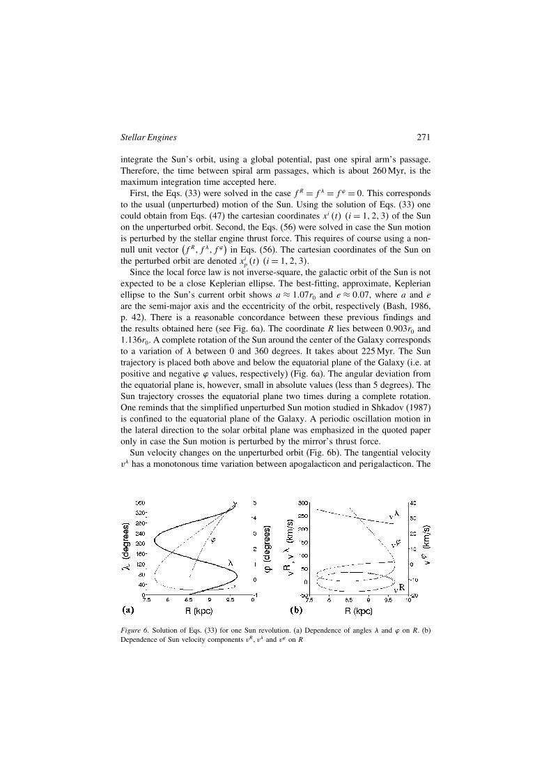
Since the local force law is not inverse-square, the galactic orbit of the Sun is notexpected to be a close Keplerian ellipse. The best-fitting, approximate, Keplerianellipse to the Sun’s current orbit shows a ≈ 1&07r0 and e ≈ 0&07, where a and eare the semi-major axis and the eccentricity of the orbit, respectively (Bash, 1986,p. 42). There is a reasonable concordance between these previous findings andthe results obtained here (see Fig. 6a). The coordinate R lies between 0&903r0 and1&136r0. A complete rotation of the Sun around the center of the Galaxy correspondsto a variation of ! between 0 and 360 degrees. It takes about 225 Myr. The Suntrajectory is placed both above and below the equatorial plane of the Galaxy (i.e. atpositive and negative " values, respectively) (Fig. 6a). The angular deviation fromthe equatorial plane is, however, small in absolute values (less than 5 degrees). TheSun trajectory crosses the equatorial plane two times during a complete rotation.One reminds that the simplified unperturbed Sun motion studied in Shkadov (1987)is confined to the equatorial plane of the Galaxy. A periodic oscillation motion inthe lateral direction to the solar orbital plane was emphasized in the quoted paperonly in case the Sun motion is perturbed by the mirror’s thrust force.

Sun velocity changes on the unperturbed orbit (Fig. 6b). The tangential velocityv! has a monotonous time variation between apogalacticon and perigalacticon. The

Figure 6. Solution of Eqs. (33) for one Sun revolution. (a) Dependence of angles ! and " on R. (b)Dependence of Sun velocity components vR%v! and v" on R


radial velocity vR reaches its extreme values near R = r0. The time variation of v!

is slightly more complicated.A stellar engine thrust force of constant magnitude will be considered in the

following. The perturbed motion of the Sun depends, of course, on the direction ofthe thrust force. Three simple strategies of changing Sun movement are defined now.In the first case the thrust force is constantly acting on the (outward) direction ofR and it corresponds to fR = 1" f # = f! = 0 in Eqs. (56). The second case corre-sponds to f! = 1" fR = f # = 0 and refers to a thrust force constantly acting onthe direction of the generalized variable !. A thrust force constantly acting on thedirection of the generalized variable # (i.e.f # = 1" fR = f! = 0$ is the third strategy.

In all the three above cases the time-dependent distance %R &t$ between theperturbed and unperturbed positions of the Sun, respectively, is defined in the usualway as

(58) %R &t$ ≡!"

x1p −x1

#2 +"x2

p −x2#2 +

"x3

p −x3#2$1/2

'

The time dependence of %R is shown in Fig. 7 for the three strategies. A singlerotation of the Sun around the center of the Galaxy was considered. The distance %Rdepends on the direction of the thrust force (i.e. on the strategy), as expected. Noneof the three strategies make the distance between the perturbed and the unperturbedSun position increase linearly in time. An optimal control strategy for the thrustforce direction is required for this purpose. The second strategy (i.e. f # = 1$ yieldsthe largest values of %R during the time interval considered here. The deviationfrom the unperturbed orbit could be as large as 40 pc. Note the maximum %R isobtained with the fR = 1 strategy about 140 Myr after stellar engine implementation.

Figure 7. Time variation of distance %R &t$ between the perturbed and unperturbed positions of the Sun,respectively, during one Sun galactic revolution. Solutions of Eqs. (56) were used. Three strategies ofchanging Sun movement are considered: (i) fR = 1 (stellar engine thrust force is acting on the (outward)direction of R), (ii) f# = 1 (thrust force acting on the direction of #$, (iii) f! = 1 (thrust force actingon the direction of !$

Stellar Engines 273

It is interesting to compare our findings with early results obtained in Shkadov(1987) by using a simplified analytical model. In the quoted paper the mirror axisforms a right angle with the radius-vector of the Sun that is assumed to move ona circular orbit in the equatorial plane of the Galaxy. This means that the thrustvector is always acting in the equatorial plane of the Galaxy and it is directed alongthe tangent to the solar orbit. In Shkadov (1987) the radius of the circular orbit ofthe Sun is estimated to 10 kpc while the period of one Sun revolution in the Galaxyis assumed to be 200 Myr. The quoted author found a Sun radial deviation from itsorbit of about 12 pc. This is about three times smaller than the results obtained inthis chapter by using a more accurate treatment.

4.3 Second Galaxy Gravitational Potential

Another axi-symmetric gravitational potential per unit mass of the solar system,! "r# $# z%, will be used in this section. It consists of a disk-halo Plummer potentialsupplemented with some spherical potentials (see Carlberg and Innanen, 1987):

(59)

! "r# $# z% =− &1Meff g!"

a+3#

i=1'i

$z2 +h2

i

%1/2&2

+b21 + r2

'1/2 −4#

j=2

&jMeff g$b2

j + r2%1/2 (

Here a cylindrical system of coordinates "r# $# z% was used. Other notations in Eq. (59)are: g

$= 6(67 ·10−11m3kg−1s−2

%is the gravitational constant, Meff = 9(484 ·1011MS

is the effective Galaxy mass influencing Sun’s movement, &j "j = 1# 2# 3# 4% are massweighting coefficients for various potential components, a and b1 are the scale lengthand the core radius of the disk-halo, respectively, 'i "i = 1# 2# 3% and hi "i = 1# 2# 3%correspond to the scale heights of various disk-halo components while bj "j = 2# 3# 4%are the core radii of the additional spherical potentials (for bulge, nucleus and darkhalo, respectively). Table 1 shows the data.

Table 1. Data for the Galaxy gravitational potential of (Carlberg and Innanen, 1987)

Componentj

Disk-halo"j = 1%

Bulge"j = 2%

Nucleus"j = 3%

Dark-halo"j = 4%

&j 0.1554 0.0490 0.0098 0.7859bj (kpc) 8.0 3.0 0.25 35.0a (kpc) 3.0 0 0 0'1 0.4 0 0 0'2 0.5 0 0 0'3 0.1 0 0 0h1 (kpc) 0.325 0 0 0h2 (kpc) 0.090 0 0 0h3 (kpc) 0.125 0 0 0


The components of the gradient of ! in the coordinate system "r# $# z% are definedas projections of the gravitational acceleration vector G:

(60) Gr = 1Hr

&!

&r# G$ = 1

H$

&!

&$= 0# Gz = 1

Hz

&!

&z'

The Lamé coefficients Hi "i = r# $# z% are used here. One denotes the compo-nents of Sun’s velocity by vi "i = R#(#)% and one defines the new dimensionlessvariables:

(61) r ≡ r

r0vr ≡ vr

v0v$ ≡ v$

v0vz ≡ vz

v0'

In the dimensionless notation Eqs. (61), the Eqs. (51)-(52) of Sun movement are:

˙r = D1vr $ = D1

v$

r˙z = D1v

z(62a-c)

˙vr = D1

(v$)2

r(62d)

+ D4

⎧⎪⎪⎪⎪⎪⎨

⎪⎪⎪⎪⎪⎩

*1r{[a+

3∑i=1

+i

(z2 + h2

i

)1/2]2

+ b21 + r2

}3/2 +4∑

j=2

*j r(b2

j + r2)3/2

⎫⎪⎪⎪⎪⎪⎬

⎪⎪⎪⎪⎪⎭

+f rD3

˙v$ = −D1vr v$

r+f $D3(62e)

˙vz = D4

*1z

[a+

3∑i=1

+i

(z2 + h2

i

)1/2]

{[a+

3∑i=1

+i

(z2 + h2

i

)1/2]2

+ b21 + r2

}3/2

⎡

⎢⎣3∑

i=1

+i(z2 + h2

i

)1/2

⎤

⎥⎦+f zD3(62f)

Here the Eqs. (42) and (59) and following dimensionless constants were also used:

(63) a ≡ a

r0# b1 ≡ b1

r0# hi ≡ hi

r0"i = 1# 2# 3% # D4 ≡ T0Meff g

v0r20

'

In Eqs. (62) the unit vector(f r#f $#f z

)gives the direction of the thrust force F ′

(see Eq. 42) in the coordinate system "r# $# z%.The Eqs. (62) are solved numerically by using the ODE-solver SDRIV3 (Fong

et al., 1993). One assumes again that initially (i.e. at time t = 0% the Sun isfound in the equatorial plane of the Galaxy. This makes possible to use the sameinitial conditions we used in Section 4.1. In cylindrical coordinates, this meansr "t = 0% = r0, $ "t = 0% = 0 and z "t = 0% = 0. The components of the initial Sunvelocity are: vr "t = 0% = u0 +U0, v$ "t = 0% = v0 +V0 and vz "t = 0% = w0 +W0.

Stellar Engines 275

To solve the unperturbed motion of the Sun requires using f r = f ! = f z = 0 inEqs. (62). Results are shown in Fig. 8. The coordinate r lies between 0"942r0 and1"193r0. This is in reasonably good agreement with results given in Bash (1986),where an approximate Sun motion confined to the galactic mid-plane was studied.A perturbation potential due to standard spirals pattern was however included inthat model. The perturbation potential was assumed to be 5% of the global axi-symmetric potential. The initial values were slightly different from those we usedhere. One found that the Sun reaches perigalacticon at r = 0"995r0 and apogalacticonat r = 1"145r0, where r0 is the initial value of r used in Bash (1986).

A complete rotation of the Sun around the center of the Galaxy (that correspondsto a variation of ! between 0 and 360 degrees) takes about 248.5 Myr. This is about10 % longer than in case of the gravitational potential used in section 4.1.

The rotation motion of the Sun is qualitatively similar for both Galaxy grav-itational potentials we considered in this paper (compare Fig. 8 and Fig. 6,respectively). Differences exist however in the predictions about the vertical motion.

A usual simplified orbit integration procedure is to separate the motion in themid-galactic plane from the Sun’s vertical motion. Sometimes the last motion ismodeled as a simple harmonic oscillation. A vertical oscillation period of 66 Myrwas accepted, for example, in Bash (1986). In this case the Sun would cross the mid-plane every 33 Myr, i.e. between seven and eight times during a complete revolution.

In the present work there is no decomposition of Sun motion and, therefore,more accurate results are expected. Figure 8a shows that the Sun deviation fromthe equatorial plane of the Galaxy lies between −80 pc and +80 pc and the Suntrajectory crosses the equatorial plane four times during a complete revolution.

Note that in Gonzalez (1999) one estimates that the Sun spends most of itstime at least 40 pc from the Galactic mid-plane. Also, some studies reported forthe maximum distance zmax between the Sun and Galaxy’s equatorial plane valuesranging from 76.8 to 81.8 pc (Bash, 1986), which is in good concordance with ourresults.

Figure 8. Solution of Eqs. (62) for one Sun revolution. (a) Dependence of variables ! and z on r .(b) Dependence of Sun velocity components vr #v! and vz on r


Figure 9. Time variation of the distance !R "t# between the perturbed and unperturbed positions of theSun, respectively, during one Sun galactic revolution. Solutions of the equations system (62) were used.Three strategies of changing Sun movement are considered: (i) f r = 1 (stellar engine thrust force isacting on the (outward) direction of r#, (ii) f $ = 1 (thrust force acting on the direction of the generalizedvariable $#, (iii) f z = 1 (thrust force acting on z direction)

The tangential velocity v$ and the radial velocity vr have a monotonous timevariation between their minimum and maximum values but the time variation of vz

is slightly more complicated (Fig. 8b).Three simple strategies of changing Sun movement are again considered here.

In the first case the stellar engine thrust force is constantly acting on the (outward)direction of r and it corresponds to f r = 1% f $ = f z = 0 in Eqs. (62). The secondcase corresponds to f $ = 1% f r = f z = 0 and refers to a thrust force constantlyacting on the direction of the generalized variable $. A thrust force acting on zdirection (i.e. f z = 1% f r = f $ = 0) is the third strategy.

The time-dependent distance !R "t# between the perturbed and unperturbed posi-tions of the Sun is defined by Eq. (58).

Figure 9 shows the time dependence of !R during one Sun revolution for the threestrategies defined above. The second strategy (i.e. f $ = 1) yields the largest valuesof !R. The maximum deviation from the unperturbed orbit is about 35 pc. This isin good agreement with the result obtained by using the gravitational potential ofsection 4.1 (compare Fig. 9 and Fig. 7, respectively).

5. CONCLUSIONS

A stellar engine is defined in this chapter as a device that uses an important partof star resources to produce work. A classification is proposed as follows. A classA stellar engine uses the impulse of the radiation emitted by a star to produce athrust force. When acting on a finite distance the thrust force generates work. ClassA stellar engines can be used for interstellar travel. As example we quote the Sun

Stellar Engines 277

thruster proposed by Shkadov (1987). A class B stellar engine uses the energy ofthe radiation emitted by a star to generate mechanical power. It is based on theconcept of the Dyson sphere (DS). As example we cite the stellar engine proposedin Badescu (1995). A class C stellar engine is a combination between class A andclass B stellar engines and provides a Kardashev type II civilisation with bothpower and the possibility of interstellar travel.

A class A stellar engine is associated with an increase in the affected star’sphotosphere temperature. For instance, by increasing the mirror’s rim angle from 0to 90 degrees the spectral class of the Sun changes from G2 towards F2. However,a reasonable rim angle value (! = 30!" keeps the photosphere temperature (and itsassociated spectral class) quite close to the present-day values.

A number of conclusions may be drawn regarding the manufacturing of a classB stellar engine in our solar system. First, small radii increase the feasibility ofthe project as the amount of material required is proportional to the square of theradius. Second, the inner planets seem to be the best source of material because ofthe shorter distance between their orbit and the place of the future construction.

The efficiency of a class C stellar engine increases by increasing its radius anddecreasing the mirror rim angle ! . There is a minimum radius for such engine toprovide useful power. The important fact is that there is an optimum stellar engineradius as far as the provided power density is concerned. For values adopted herethis optimum radius is around 450 millions km (see Fig. 4c).

The mirror of class A and class C stellar engines makes the Sun’s temperatureincrease and this has consequences on the thrust force acting on the Sun. In bothcases the thrust force F increases by increasing the mirror rim angle ! , as expected.The thrust force of the class A stellar engine is, however, larger than first esti-mated by Shkadov (1987) without taking into account the increase in the Sun’stemperature.

Changing into a controllable way the trajectory of the Sun in the Galaxy is ofgreat potential interest for humanity. In this chapter we have studied in some detailhow class A or class C stellar engines could be used for this purpose. One hasproved in Section 3.4 that both types of stellar engines provide practically the samethrust force when used to change Sun orbit.

A simple dynamic model for Sun motion in the Galaxy was developed in Section4. It takes into account the (perturbation) thrust force provided by the stellar engine,which is superposed on the usual gravitational forces. The model allowed us toevaluate the distance between the perturbed position of the Sun and the usualSun position. To increase confidence in results two different Galaxy gravitationalpotential models were used in calculations. In both cases, the results obtained showsimilar qualitative features for Sun’s unperturbed motion.

Three simple strategies of changing Sun orbit were considered. A constant modulethrust force was always assumed and the difference consisted in the force direction.None of these strategies make the distance between the perturbed and the unper-turbed Sun position increase linearly in time. For this purpose an optimal controlstrategy is to be used.


For a single Sun revolution the maximum estimated deviation is between 35 and40 pc (depending on the gravitational potential involved). Both Fig. 7 and Fig. 9show that the stellar engine gives a 10 pc deviation of the Sun in less than 150 Myr.The number density of stars in the solar neighborhood is about 0.104 per cubicpc and so within a 10 pc radius sphere we would find around 400 stars, about 10of which would be single solar-type stars (see e.g. (Fogg, 1995, p. 461)). Thisgives some perspective to future interstellar transfer macro-projects. The durationinvolved is, however, large and other kinds of stellar engines than those we studiedmust also be considered. One concludes that class A or class C stellar engines maybe used to control in a certain extent the Sun’s movement in the Galaxy.

ACKNOWLEDGMENTS

This work is dedicated to our friend Henrik Farkas (Technical University ofBudapest) who passed away on 21 July 2005.

REFERENCES

Badescu V (1993) Maximum concentration ratio of direct solar radiation. Appl Optics 32(12):2187–2189Badescu V (1995) On the radius of the Dyson sphere. Acta Astronautica 36:135–138Badescu V (2004) Simulation of a solar Stirling engine operation under various weather conditions on

Mars. J Solar Energy Eng 126:812–818Badescu V, Cathcart RB (2000) Stellar engines for Kardashev’s type II civilisations. J Br Interplanet

Soc 53:297–306Badescu V, Cathcart RB (2006) Use of class A and class C stellar engines to control sun movement in

the galaxy. Acta Astronautica 58:119–129Bash F (1986) The present, past and future velocity of nearby stars: the path of the Sun in 108 years. In:

Smoluchowski R, Bahcall JN, Matthews MS (eds) The Galaxy and the Solar System. The Universityof Arizona Press, Tucson

Bejan A (1996) Entropy generation minimization: the new thermodynamics of finite-size devices andfinite-time processes. J Appl Phys 79:1191–1218

Beju I, Soos E, Teodorescu PP (1976) Tehnici de Calcul Vectorial Cu Aplicatii, Editura Tehnica,Bucuresti

Bienayme O (1999) The local stellar velocity of the galaxy: galactic structure and potential. AstronomyAstrophysics 341:86–97

Carlberg RG, Innanen KA (1987) Galactic chaos and the circular velocity at the sun. Astron J 94:666–670Clube SVM, Napier WM (1984) Terrestrial catastrophism: Nemesis or galaxy? Nature 311:635–636Criswell DR (1985) Solar system industrialization: implications for interstellar migrations. In: Finney

R, Jones EM (eds) Interstellar Migration and the Human Experience. University of California Press,Berkeley, pp 50–87

Darling D (2004) The Universal Book of Astronomy. Wiley, New York, pp 456De Vos A (1985) Efficiency of some heat engines at maximum-power conditions. Am J Phys

53(5):570–573Dehnen MW, Binney JJ (1998) Local stellar kinematics from HIPPARCOS data. Monthly Notices Royal

Astronom Society 298:387–394Dyson FJ (1966) The search for extraterrestrial technology. In: Marshak RE (ed) Perspectives in modern

physics. Interscience Publishers, New York, pp 641–655Fogg MJ (1989) Solar exchange as a means of ensuring the long term habitability of the Earth. Spec

Sci Technol 12:153–157

Stellar Engines 279

Fogg MJ (1995) Terraforming: Engineering Planetary Environments. SAE, WarrendaleFong KW, Jefferson TH, Suyehiro T, Walton L (1993) Guide to the SLATEC common mathematical

library. Energy Science and Technology Software Center, PO Box 1020, Oak Ridge, TN 37831, USAGonzalez G (1999) Is the Sun anomalous? Astronomy Geophys 40:5.25–5.25.29Hills JG (1984) Close encounters between a star-planet system and a stellar intruder. Astron J

89:1559–1564Hoffmann KH, Burzler JM, Schubert E (1997) Endoreversible Thermodynamics. J Non-Equilib Ther-

modyn 22:311–355Infante F (1992) Projects for the reconstruction of the firmament. Leonardo 25:11Jones EM (1981) Discrete calculations of interstellar migration and settlement. Icarus 46:328–336Kardashev NS (1964) Transmission of information by extraterrestrial civilisations, Astron Zh 8:217Kasting JF (1988) Runaway and moist greenhouse atmospheres and the evolution of Earth and Venus.

Icarus 74:472–494Knill O (2003) Moving the solar system. http://www.dynamical.systems.org/zwicky/Essay.htmlKorykansky DG (2004) Astroengineering, or how to save the Earth in only one billion years. Rev Mex

A A (Serie Conferencias) 22:117–120Korykansky DG, Laughlin G, Adams FC (2001) Astronomical engineering: a strategy for modifying

planetary orbits. Astrophys Sp Sci 275:349–366Kovalevsky J (1999) First results from HIPPARCOS. Annu Rev Astronomy Astrophys 36:99–130Landsberg PT, Badescu V (1998) Solar energy conversion: list of efficiencies and some theoretical

considerations. Part I – Theoretical considerations. Prog Quantum Electronics 22:211–230McInnes CR (2002) Astronomical engineering revisited: planetary orbit modification using solar radiation

pressure. Astrophys Sp Sci 282:765–772Mishunov Yu N, Zenina IA (1999) Yes, the Sun is located near the corotation circle. Astronomy

Astrophys 341:81–85Moore P (1970) Atlas of the Universe. Mitchell Beazley Ltd, London, pp 35,155,159,169Nakajima S, Hayashi YY, Abe Y (1992) A study of the ‘runaway greenhouse effect’ with a one-

dimensional radiative convective equilibrium model. J Atmos Sci 49:2256Napier WN (1985) Comet formation in molecular clouds. Icarus 62:384Newman WI, Sagan C (1981) Galactic civilizations: population dynamics and interstellar diffusion.

Icarus 46:293–327Pal A, Ureche V (1983) Astronomie. Ed. Didactica si Pedagogica, Bucharest, pp. 161Sackmann I-J, Boothroyd AI, Kraemer KE (1993) Our Sun III: Present and future. Astrophys J 418:457Shkadov LM (1987) Possibility of controlling solar system motion in the galaxy. 38th Congress of IAF,

paper IAA-87–613. Brighton, UK, October 10–17Ureche V (1987) Universul. Astrofizica, vol 2. Dacia, Cluj-NapocaZuckerman B (1985) Stellar evolution: motivation for mass interstellar migrations. Q J R Astr Soc

26:56–59Zwicky F (1957) Morphological astronomy. Springer-Verlag, Berlin, pp. 260

Documents

CHAPTER 12 - dynamical-systems.org254 V. Badescu and R.B. Cathcart Of course, this limits the trajectory of the Sun to flight courses that may not be what human civilization most wants