Chapter 11 - Duration, Convexity and ImmunizationSection 11.2 - Duration

Consider two opportunities for an investment of $1,000.

A: Pays $610 at the end of year 1 and $1,000 at the end of year 3

B: Pays $450 at the end of year 1, $600 at the end of year 2 and$500 at the end of year 3.

Both have a yield rate of i = .25 because (1.25)−1 = .8,

1000 = (.8)(610) + (.8)3(1000)

and

1000 = (.8)(450) + (.8)2(600) + (.8)3(500).

11-1

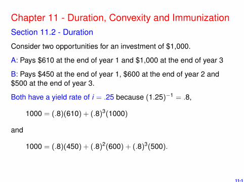
The repayment patterns of these two investments are quite differentand we seek to compare them on the basis of the timing of therepayments. Getting the repayments sooner would be advantageousif reinvestment yield rates are above the current yield of thisinvestment (in the above setting i = .25), whereas delaying therepayments is advantageous if the reinvestment interest rates arelower than the current yield rate.

Method of Equated Time (See section 2.4) provides a simple answerto measure the timing of the repayments:

Here Rt denotes a return (Rt > 0 is a payment back to the investormade at time t ).

11-2

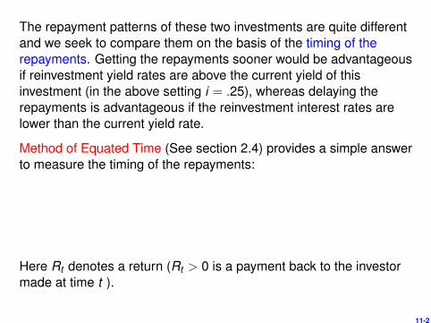
Example: (from page 11-1)

A : t = 1(610)+3(1000)610+1000 = 2.24

B : t = 1(450)+2(600)+3(500)450+600+500 = 2.03.

The money is returned faster under investment B.- - - - - - - - - - -

A better index would also take into account the current value of thefuture repayments:

Macaulay Duration:

Here the investment yield rate is used in ν. The quantity d is adecreasing function of i .

11-3

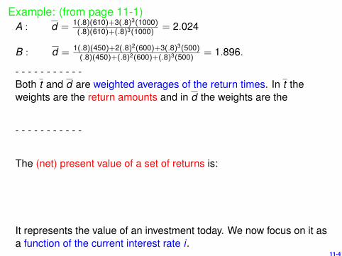
Example: (from page 11-1)A : d = 1(.8)(610)+3(.8)3(1000)

(.8)(610)+(.8)3(1000) = 2.024

B : d = 1(.8)(450)+2(.8)2(600)+3(.8)3(500)(.8)(450)+(.8)2(600)+(.8)3(500) = 1.896.

- - - - - - - - - - -Both t and d are weighted averages of the return times. In t theweights are the return amounts and in d the weights are the

- - - - - - - - - - -

The (net) present value of a set of returns is:

It represents the value of an investment today. We now focus on it asa function of the current interest rate i .

11-4

Since interest rates frequently change, the volatility of the presentvalue to changes in i is very important. It is measured with

Volatility:

The minus sign is included because P(i) is a decreasing function of iand hence P ′(i) < 0. So including the minus sign makes the ν valuepositive and therefore makes larger values of ν indicate morevolatility (susceptibility to changes in i), relative to the magnitude ofP(i).

We now relate volatility to duration by examining their definingexpressions.

11-5

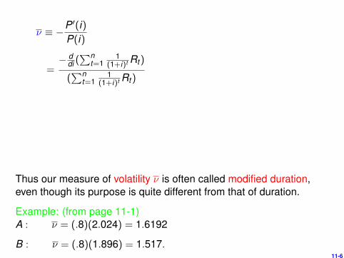
ν ≡ −P ′(i)P(i)

=− d

di (∑n

t=11

(1+i)t Rt)

(∑n

t=11

(1+i)t Rt)

Thus our measure of volatility ν is often called modified duration,even though its purpose is quite different from that of duration.

Example: (from page 11-1)A : ν = (.8)(2.024) = 1.6192

B : ν = (.8)(1.896) = 1.517.11-6

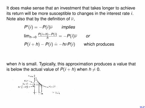
It does make sense that an investment that takes longer to achieveits return will be more susceptible to changes in the interest rate i .Note also that by the definition of ν,

P ′(i) = −P(i)ν implies

limh→0P(i+h)−P(i)

h = −P(i)ν or

P(i + h)− P(i) .= −hνP(i) which produces

when h is small. Typically, this approximation produces a value thatis below the actual value of P(i + h) when h 6= 0.

11-7

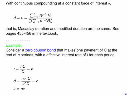
With continuous compounding at a constant force of interest δ,

d = ν =

∑nt=1 te−δtRt

(∑n

t=1 e−δtRt)

that is, Macaulay duration and modified duration are the same. Seepages 455-456 in the textbook.

- - - - - - - - - - -Example:Consider a zero coupon bond that makes one payment of C at theend of n periods, with a effective interest rate of i for each period.

t =nCC

= n

d =nνnCνnC

= n

ν = nν11-8

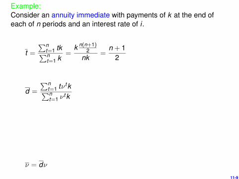
Example:Consider an annuity immediate with payments of k at the end ofeach of n periods and an interest rate of i .

t =∑n

t=1 tk∑nt=1 k

=k n(n+1)

2nk

=n + 1

2

d =

∑nt=1 tν tk∑nt=1 ν

tk

ν = dν

11-9

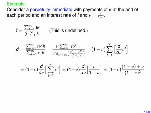
Example:Consider a perpetuity immediate with payments of k at the end ofeach period and an interest rate of i and ν = 1

1+i .

t =∑∞

t=1 tk∑∞t=1 k

(This is undefined.)

d =

∑∞t=1 tν tk∑∞t=1 ν

tk=

ν∑∞

t=1 tν t−1

limn→∞(ν(1−νn)

(1−ν) )= (1− ν)

∞∑t=1

[ ddν

ν t]

= (1−ν) ddν

[ ∞∑t=1

ν t]= (1−ν) d

dν

[ ν

1− ν

]= (1−ν)(1− ν) + ν

(1− ν)2

11-10

Exercise 11-6: The current price of an annual coupon bond is 100.The derivative of the price of the bond with respect to the yield tomaturity is -650. The yield to maturity is an effective rate of 7%.(a) Calculate the Macaulay duration of the bond.(b) Estimate the price of the bond using the approximation formula

on page 11-7 when the yield is 8% instead of 7%.

11-11

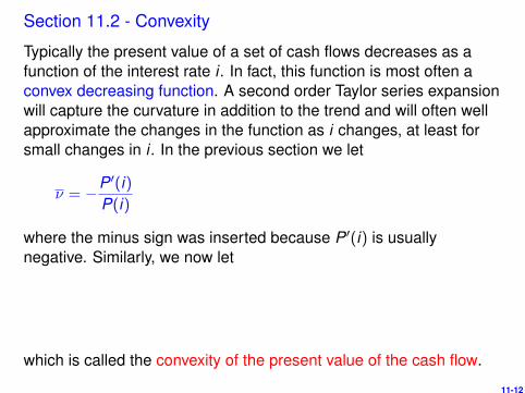
Section 11.2 - Convexity

Typically the present value of a set of cash flows decreases as afunction of the interest rate i . In fact, this function is most often aconvex decreasing function. A second order Taylor series expansionwill capture the curvature in addition to the trend and will often wellapproximate the changes in the function as i changes, at least forsmall changes in i . In the previous section we let

ν = −P ′(i)P(i)

where the minus sign was inserted because P ′(i) is usuallynegative. Similarly, we now let

which is called the convexity of the present value of the cash flow.

11-12

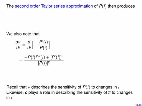
The second order Taylor series approximation of P(i) then produces

We also note that

dνdi

=ddi

[− P ′(i)

P(i)

]

=−P(i)P ′′(i) + [P ′(i)]2

[P(i)]2

Recall that ν describes the sensitivity of P(i) to changes in i .Likewise, c plays a role in describing the sensitivity of ν to changesin i .

11-13

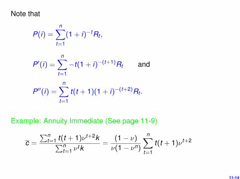
Note that

P(i) =n∑

t=1

(1 + i)−tRt ,

P ′(i) =n∑

t=1

−t(1 + i)−(t+1)Rt and

P ′′(i) =n∑

t=1

t(t + 1)(1 + i)−(t+2)Rt .

Example: Annuity Immediate (See page 11-9)

c =

∑nt=1 t(t + 1)ν t+2k∑n

t=1 νtk

=(1− ν)ν(1− νn)

n∑t=1

t(t + 1)ν t+2

11-14

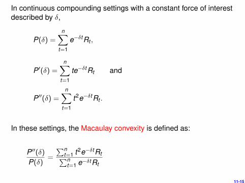
In continuous compounding settings with a constant force of interestdescribed by δ,

P(δ) =n∑

t=1

e−δtRt ,

P ′(δ) =n∑

t=1

te−δtRt and

P ′′(δ) =n∑

t=1

t2e−δtRt .

In these settings, the Macaulay convexity is defined as:

P ′′(δ)P(δ)

=

∑nt=1 t2e−δtRt∑n

t=1 e−δtRt

11-15

Exercise 11-11: A loan is to be repaid with payments of $1,000 atthe end of year 1, $2,000 at the end of year 2, and $3,000 at the endof year 3. The effective rate of interest is i = .25. Find (a) theamount of the loan, (b) the duration, (c) the modified duration, and(d) the convexity.

11-16

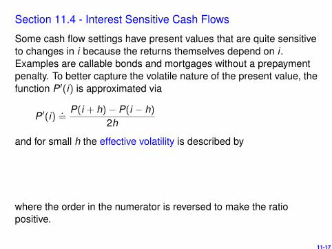
Section 11.4 - Interest Sensitive Cash Flows

Some cash flow settings have present values that are quite sensitiveto changes in i because the returns themselves depend on i .Examples are callable bonds and mortgages without a prepaymentpenalty. To better capture the volatile nature of the present value, thefunction P ′(i) is approximated via

P ′(i) .=P(i + h)− P(i − h)

2h

and for small h the effective volatility is described by

where the order in the numerator is reversed to make the ratiopositive.

11-17

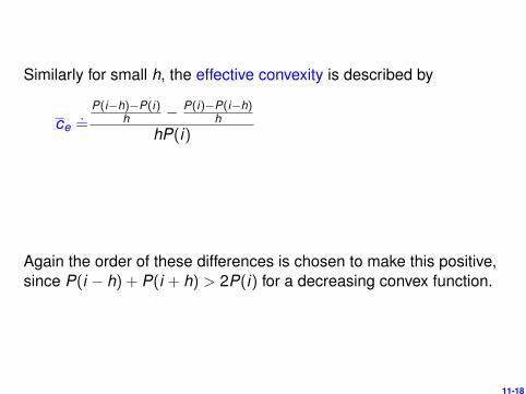
Similarly for small h, the effective convexity is described by

ce.=

P(i−h)−P(i)h − P(i)−P(i−h)

hhP(i)

Again the order of these differences is chosen to make this positive,since P(i − h) + P(i + h) > 2P(i) for a decreasing convex function.

11-18

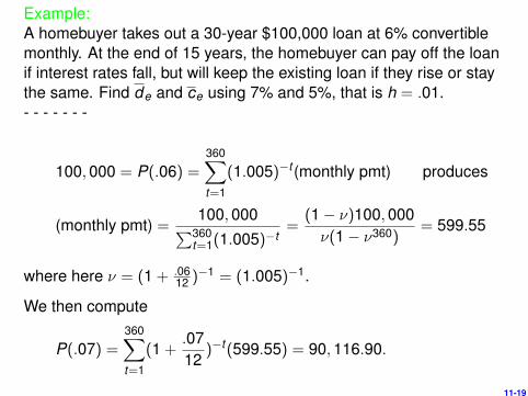
Example:A homebuyer takes out a 30-year $100,000 loan at 6% convertiblemonthly. At the end of 15 years, the homebuyer can pay off the loanif interest rates fall, but will keep the existing loan if they rise or staythe same. Find de and ce using 7% and 5%, that is h = .01.- - - - - - -

100,000 = P(.06) =360∑t=1

(1.005)−t (monthly pmt) produces

(monthly pmt) =100,000∑360

t=1(1.005)−t=

(1− ν)100,000ν(1− ν360)

= 599.55

where here ν = (1 + .0612 )−1 = (1.005)−1.

We then compute

P(.07) =360∑t=1

(1 +.0712

)−t(599.55) = 90,116.90.

11-19

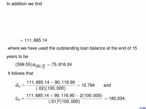
In addition we find

= 111,685.14

where we have used the outstanding loan balance at the end of 15

years to be

(599.55)a180| .0512

= 75,816.24.

It follows that

de.=

111,685.14− 90,116.90(.02)(100,000)

= 10.784 and

ce.=

111,685.14 + 90,116.90− 2(100,000)(.01)2(100,000)

= 180.204.

11-20

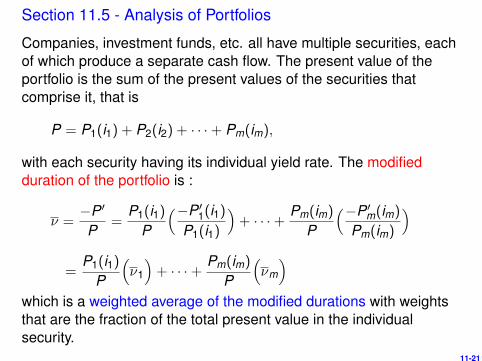
Section 11.5 - Analysis of Portfolios

Companies, investment funds, etc. all have multiple securities, eachof which produce a separate cash flow. The present value of theportfolio is the sum of the present values of the securities thatcomprise it, that is

P = P1(i1) + P2(i2) + · · ·+ Pm(im),

with each security having its individual yield rate. The modifiedduration of the portfolio is :

ν =−P ′

P=

P1(i1)P

(−P ′1(i1)P1(i1)

)+ · · ·+ Pm(im)

P

(−P ′m(im)Pm(im)

)=

P1(i1)P

(ν1

)+ · · ·+ Pm(im)

P

(νm

)which is a weighted average of the modified durations with weightsthat are the fraction of the total present value in the individualsecurity.

11-21

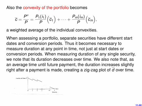
Also the convexity of the portfolio becomes

c =P ′′

P=

P1(i1)P

(c1

)+ · · ·+ Pm(im)

P

(cm

),

a weighted average of the individual convexities.

When assessing a portfolio, separate securities have different startdates and conversion periods. Thus it becomes necessary tomeasure duration at any point in time, not just at start dates orconversion periods. When measuring duration of any single security,we note that its duration decreases over time. We also note that, asan average time until future payment, the duration increases slightlyright after a payment is made, creating a zig-zag plot of d over time.

11-22

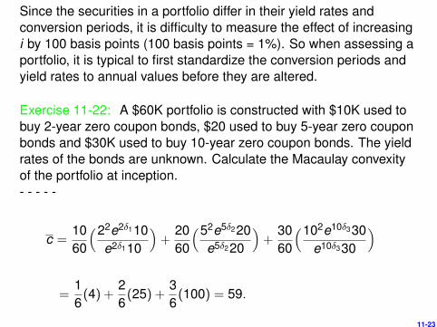
Since the securities in a portfolio differ in their yield rates andconversion periods, it is difficulty to measure the effect of increasingi by 100 basis points (100 basis points = 1%). So when assessing aportfolio, it is typical to first standardize the conversion periods andyield rates to annual values before they are altered.

Exercise 11-22: A $60K portfolio is constructed with $10K used tobuy 2-year zero coupon bonds, $20 used to buy 5-year zero couponbonds and $30K used to buy 10-year zero coupon bonds. The yieldrates of the bonds are unknown. Calculate the Macaulay convexityof the portfolio at inception.- - - - -

c =1060

(22e2δ110e2δ110

)+

2060

(52e5δ220e5δ220

)+

3060

(102e10δ330e10δ330

)

=16(4) +

26(25) +

36(100) = 59.

11-23

Exercise 11-20:A 3-year loan at 10% effective is being repaid with level annualpayments at the end of each year.(a) Calculate the jump in duration at the time of the first payment.(b) Rework (a) at the time of the second payment.(c) Compare the answers to (a) and (b) and verbally explain therelationship.

11-24

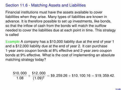
Section 11.6 - Matching Assets and Liabilities

Financial institutions must have the assets available to coverliabilities when they arise. Many types of liabilities are known inadvance. It is therefore possible to set up investments, like bonds,so that the inflow of cash from the bonds will match the outflowneeded to cover the liabilities due at each point in time. This strategyis called

Example A company has a $10,000 liability due at the end of year 1and a $12,000 liability due at the end of year 2. It can purchase1-year zero coupon bonds at 8% effective and 2-year zero couponbonds at 9% effective. What is the cost of implementing an absolutematching strategy today?

$10,0001.08

+$12,000(1.09)2 = $9,259.26 + $10,100.16 = $19,359.42.

11-25

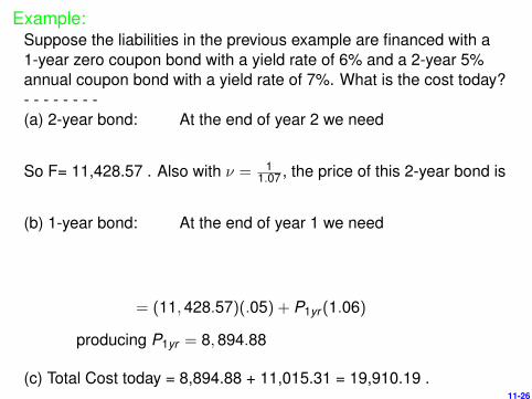
Example:Suppose the liabilities in the previous example are financed with a1-year zero coupon bond with a yield rate of 6% and a 2-year 5%annual coupon bond with a yield rate of 7%. What is the cost today?- - - - - - - -(a) 2-year bond: At the end of year 2 we need

So F= 11,428.57 . Also with ν = 11.07 , the price of this 2-year bond is

(b) 1-year bond: At the end of year 1 we need

= (11,428.57)(.05) + P1yr (1.06)

producing P1yr = 8,894.88

(c) Total Cost today = 8,894.88 + 11,015.31 = 19,910.19 .11-26

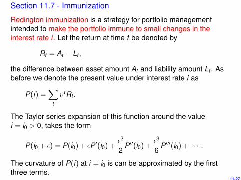
Section 11.7 - Immunization

Redington immunization is a strategy for portfolio managementintended to make the portfolio immune to small changes in theinterest rate i . Let the return at time t be denoted by

Rt = At − Lt ,

the difference between asset amount At and liability amount Lt . Asbefore we denote the present value under interest rate i as

P(i) =∑

t

ν tRt .

The Taylor series expansion of this function around the valuei = i0 > 0, takes the form

P(i0 + ε) = P(i0) + εP ′(i0) +ε2

2P ′′(i0) +

ε3

6P ′′′(i0) + · · · .

The curvature of P(i) at i = i0 is can be approximated by the firstthree terms.

11-27

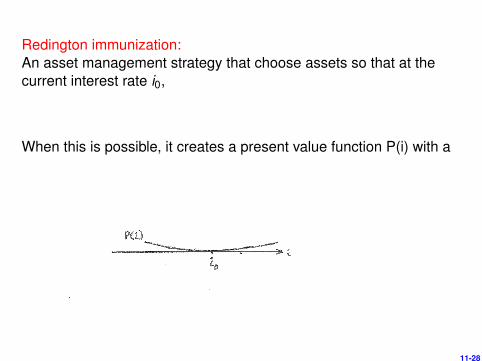
Redington immunization:An asset management strategy that choose assets so that at thecurrent interest rate i0,

When this is possible, it creates a present value function P(i) with a

11-28

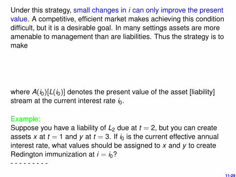
Under this strategy, small changes in i can only improve the presentvalue. A competitive, efficient market makes achieving this conditiondifficult, but it is a desirable goal. In many settings assets are moreamenable to management than are liabilities. Thus the strategy is tomake

where A(i0)[L(i0)] denotes the present value of the asset [liability]stream at the current interest rate i0.

Example:Suppose you have a liability of L2 due at t = 2, but you can createassets x at t = 1 and y at t = 3. If i0 is the current effective annualinterest rate, what values should be assigned to x and y to createRedington immunization at i = i0?- - - - - - - - -

11-29

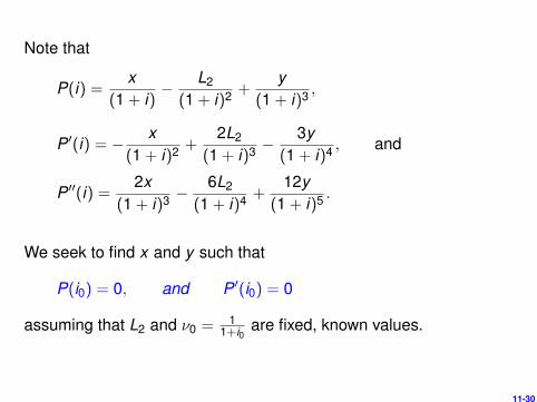
Note that

P(i) =x

(1 + i)− L2

(1 + i)2 +y

(1 + i)3 ,

P ′(i) = − x(1 + i)2 +

2L2

(1 + i)3 −3y

(1 + i)4 , and

P ′′(i) =2x

(1 + i)3 −6L2

(1 + i)4 +12y

(1 + i)5 .

We seek to find x and y such that

P(i0) = 0, and P ′(i0) = 0

assuming that L2 and ν0 = 11+i0

are fixed, known values.

11-30

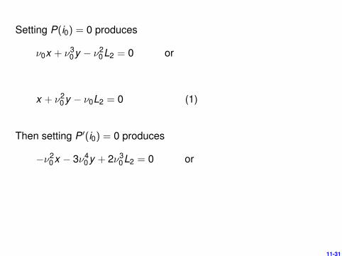
Setting P(i0) = 0 produces

ν0x + ν30y − ν2

0L2 = 0 or

x + ν20y − ν0L2 = 0 (1)

Then setting P ′(i0) = 0 produces

−ν20x − 3ν4

0y + 2ν30L2 = 0 or

11-31

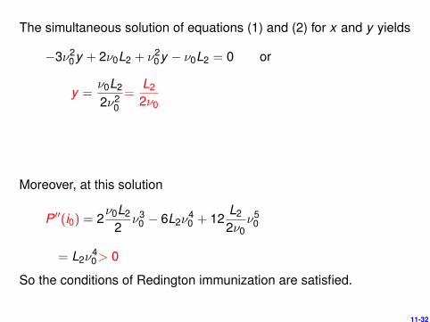
The simultaneous solution of equations (1) and (2) for x and y yields

−3ν20y + 2ν0L2 + ν2

0y − ν0L2 = 0 or

y =ν0L2

2ν20=

L2

2ν0

Moreover, at this solution

P ′′(i0) = 2ν0L2

2ν3

0 − 6L2ν40 + 12

L2

2ν0ν5

0

= L2ν40> 0

So the conditions of Redington immunization are satisfied.

11-32

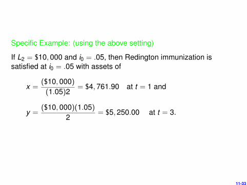
Specific Example: (using the above setting)

If L2 = $10,000 and i0 = .05, then Redington immunization issatisfied at i0 = .05 with assets of

x =($10,000)(1.05)2

= $4,761.90 at t = 1 and

y =($10,000)(1.05)

2= $5,250.00 at t = 3.

11-33

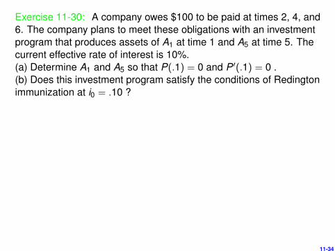
Exercise 11-30: A company owes $100 to be paid at times 2, 4, and6. The company plans to meet these obligations with an investmentprogram that produces assets of A1 at time 1 and A5 at time 5. Thecurrent effective rate of interest is 10%.(a) Determine A1 and A5 so that P(.1) = 0 and P ′(.1) = 0 .(b) Does this investment program satisfy the conditions of Redingtonimmunization at i0 = .10 ?

11-34

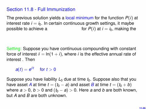
Section 11.8 - Full Immunization

The previous solution yields a local minimum for the function P(i) atinterest rate i = i0. In certain continuous growth settings, it maybepossible to achieve a for P(i) at i = i0, making the

Setting: Suppose you have continuous compounding with constantforce of interest δ = ln(1 + i), where i is the effective annual rate ofinterest . Then

a(t) = eδt for t > 0

Suppose you have liability L0 due at time t0. Suppose also that youhave asset A at time t = (t0 − a) and asset B at time t = (t0 + b)where a > 0, b > 0 and (t0 − a) > 0. Here a and b are both known,but A and B are both unknown.

11-35

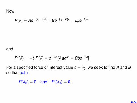
Now

P(δ) = Ae−(t0−a)δ + Be−(t0+b)δ − L0e−t0δ

and

P ′(δ) = −t0P(δ) + e−t0δ[Aaeaδ − Bbe−bδ]

For a specified force of interest value δ = δ0, we seek to find A and Bso that both

P(δ0) = 0 and P ′(δ0) = 0.

11-36

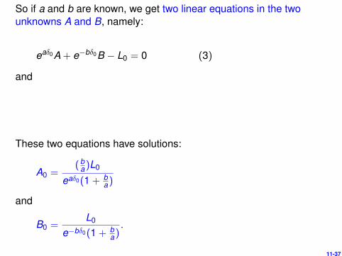
So if a and b are known, we get two linear equations in the twounknowns A and B, namely:

eaδ0A + e−bδ0B − L0 = 0 (3)

and

These two equations have solutions:

A0 =(b

a )L0

eaδ0(1 + ba )

and

B0 =L0

e−bδ0(1 + ba ).

11-37

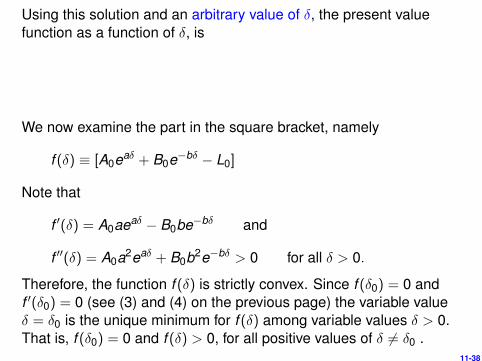
Using this solution and an arbitrary value of δ, the present valuefunction as a function of δ, is

We now examine the part in the square bracket, namely

f (δ) ≡ [A0eaδ + B0e−bδ − L0]

Note that

f ′(δ) = A0aeaδ − B0be−bδ and

f ′′(δ) = A0a2eaδ + B0b2e−bδ > 0 for all δ > 0.

Therefore, the function f (δ) is strictly convex. Since f (δ0) = 0 andf ′(δ0) = 0 (see (3) and (4) on the previous page) the variable valueδ = δ0 is the unique minimum for f (δ) among variable values δ > 0.That is, f (δ0) = 0 and f (δ) > 0, for all positive values of δ 6= δ0 .

11-38

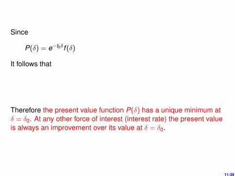
Since

P(δ) = e−t0δf (δ)

It follows that

Therefore the present value function P(δ) has a unique minimum atδ = δ0. At any other force of interest (interest rate) the present valueis always an improvement over its value at δ = δ0.

11-39

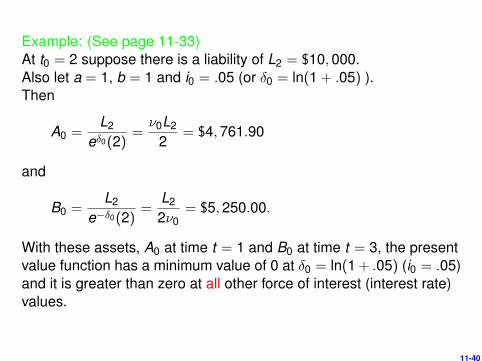
Example: (See page 11-33)At t0 = 2 suppose there is a liability of L2 = $10,000.Also let a = 1, b = 1 and i0 = .05 (or δ0 = ln(1 + .05) ).Then

A0 =L2

eδ0(2)=ν0L2

2= $4,761.90

and

B0 =L2

e−δ0(2)=

L2

2ν0= $5,250.00.

With these assets, A0 at time t = 1 and B0 at time t = 3, the presentvalue function has a minimum value of 0 at δ0 = ln(1+ .05) (i0 = .05)and it is greater than zero at all other force of interest (interest rate)values.

11-40