1

Chapter 10 Transfer between the gas-liquid interface Develop a physical picture of the air-water boundary and how it may control mass transfer Calculate mass transfer rates for water Extend these rates to other compounds Figure 10.1 page 217

2

bubbles, oil films, aerosol droplets, etc. which perturb the interface are not included in this model

3

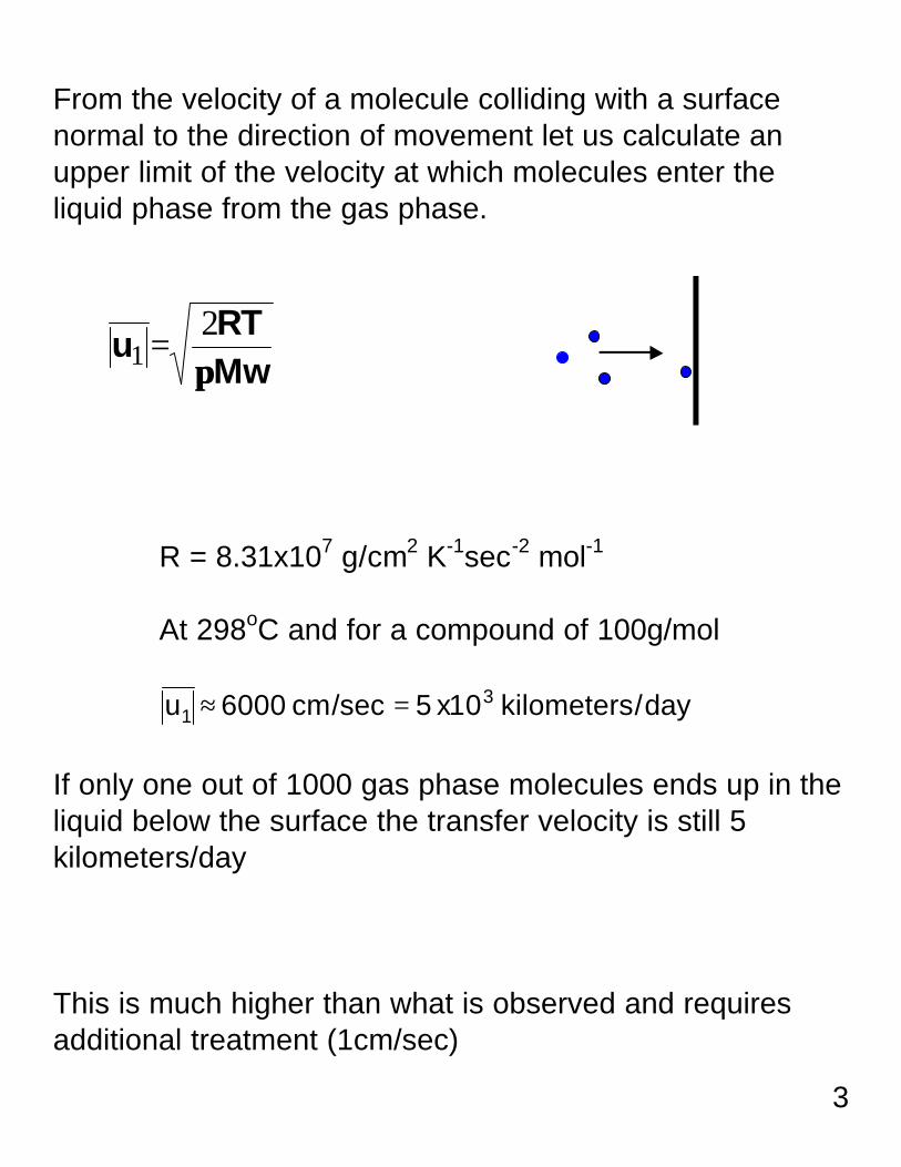
From the velocity of a molecule colliding with a surface normal to the direction of movement let us calculate an upper limit of the velocity at which molecules enter the liquid phase from the gas phase.

MwRT

uππ2

1 =

R = 8.31x107 g/cm2 K-1sec-2 mol-1 At 298oC and for a compound of 100g/mol u cm x kilometers day1

36000 5 10≈ =/sec / If only one out of 1000 gas phase molecules ends up in the liquid below the surface the transfer velocity is still 5 kilometers/day This is much higher than what is observed and requires additional treatment (1cm/sec)

4

5

The Two film model stagnant air layer Flux = -D∆C/∆z stagnant water layer Assumes that concentrations at the boundary layers are constant long enough for a concentration profile to reach steady state No chemical reactions in the boundary phases

air (well mixed)

water well mixed

6

Figure 10.2 page 220

7

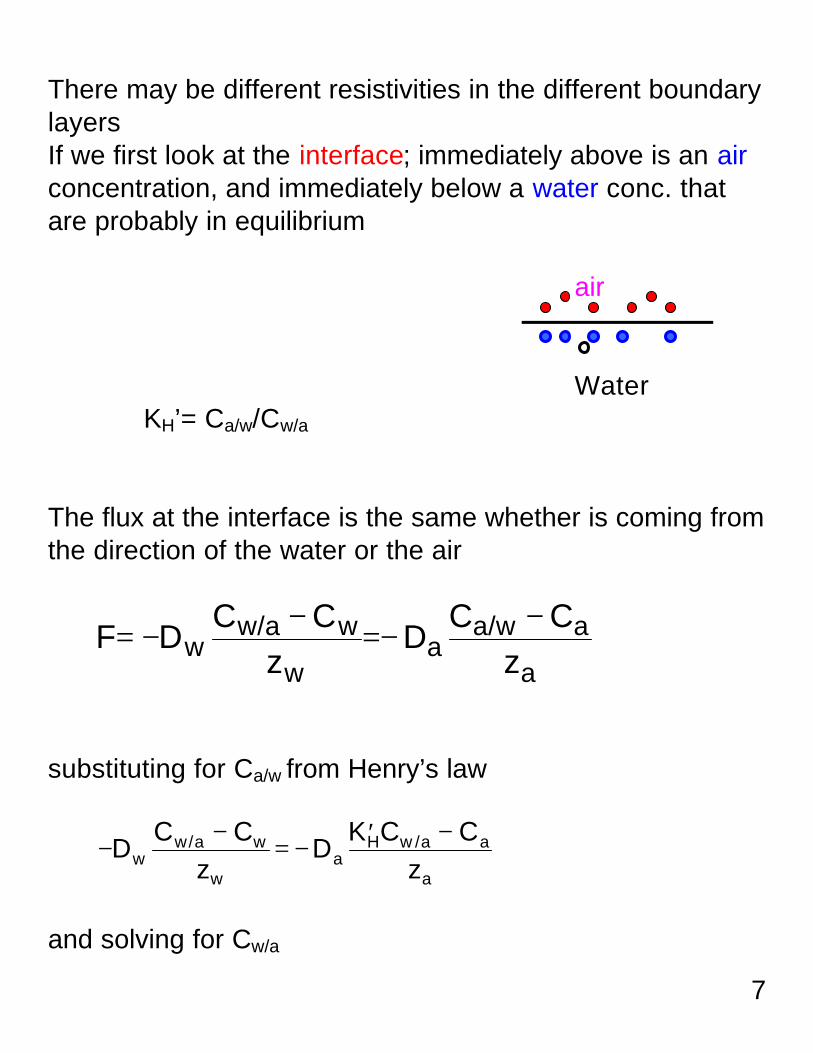
There may be different resistivities in the different boundary layers If we first look at the interface; immediately above is an air concentration, and immediately below a water conc. that are probably in equilibrium air

Water KH’= Ca/w/Cw/a

The flux at the interface is the same whether is coming from the direction of the water or the air

a

aa/wa

w

ww/aw z

CCD

zCC

DF−

−=−

−=

substituting for Ca/w from Henry’s law

−−

= − ′ −D

C Cz

DK C C

zww a w

wa

H w a a

a

/ /

and solving for Cw/a

8

CD z C D z C

D z D K zw aw w w a a a

a w a H a/

( / ) ( / )( / ) / )

=+

+ ′

CD z C D z C

D z D K zw aw w w a a a

a w a H a/

( / ) ( / )( / ) / )

=+

+ ′

recalling the expression for flux in the liquid boundary

w

ww/aw z

CCDF

−−=

and substituting we get an expression which includes mass transfer through both boundary layers

Fz D z D K

CCKw w a a H

wa

H

=+ ′

−

′

1( / ) / )

If the bulk water conc. equals Ca/K’H; which means K’H= Ca/Cw ie Ca and Cw are in equilibrium there will be no net flux

9

If the bulk water conc. > Ca/K’H; ie. Cw > Ca/K’H then F will be positive and there will be a net flow from the water to the air phase and vice versa

10

Fz D z D K

CCKw w a a H

wa

H

=+ ′

−

′

1( / ) / )

moles/(cm2 sec) cm/sec moles/cm3

w

ww/aw z

CCDF

−−=

where this net velocity flux, vtot, is called a mass transfer coef

′+

=)/)/(

1

Haawwtot KDzDz

v

note that zw/Dw has the units of sec/cm or inverse velocity

′+

=)/1)/1(

1

Hawtot Kvv

v

1/vtot= 1/vw + 1/(vaK’H )

11

12

′+

=)/1)/1(

1

Hawtot Kvv

v

1/vtot= 1/vw+ 1/(vaK’H) This has the “look and feel” of resistors in parallel 1/Rtot= 1/R1 + 1/R2

Rtot R1 R2 if vw is << vaKH vtot ~ vw

and transfer will be dominated by the water boundary layer or the resistance will be in the water layer if vw >> vaKH

13

resistance will be in air boundary layer and vtot~ vaKH

Boundary layer theory assumptions

1. We don’t know much about z thicknesses as air velocities increase we would expect the thickness of za and zw to decrease, and this is observed in that as volatilization increases so does transfer from the water to that air phase 2. It is assumed that no reactions take place in the boundary layer

What is the time needed to traverse the boundary layer compared to reaction times? σx = (2Dt)1/2

dropping the 2 in the water layer τw= zw

2/Dw and zw/Dw = 1/vw

so τw= zw/vw

14

in the air boundary τa= za/va

15

Typical lengths for zw are 5x10-2 to 5x10-3 cm and Dw = 10-5cm2/sec; this gives τw= zw

2/Dw= and for τa= For PAH reacting in sunlight in the air or on particles dPAH/PAH = -k PAH; k = ~0.02 min-1

τr ~ 1/k= 3000 sec

3. It is assumed that the bulk concentrations in air and water “above and below” the boundary layers are constant long enough to establish a steady state gradient. What if they are not?

16

Surface Renewal Model This model attempts to describe a continual turnover at the air water interface. • Eddies in the water and air immediately above and below

the air water interface transport material from the bulk phase to an interface boundary

• Henry’s law equilibrium at the interface is rapidly re-established

• Mass transported across the interface does not remain there and is mixed into the bulk phase on the other side.

Figure 10.4 page 225

17

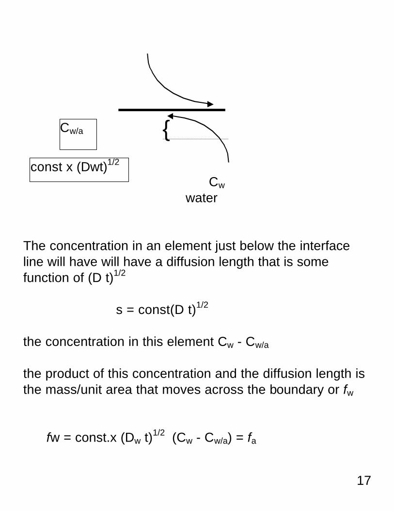
{ Cw water The concentration in an element just below the interface line will have will have a diffusion length that is some function of (D t)1/2 s = const(D t)1/2 the concentration in this element Cw - Cw/a

the product of this concentration and the diffusion length is the mass/unit area that moves across the boundary or fw fw = const.x (Dw t)1/2 (Cw - Cw/a) = fa

Cw/a

const x (Dwt)1/2

18

fa = const.x(Da t)1/2(Ca/w - Ca)

19

const.x (Dw t)1/2 (Cw - Cw/a) = const.x(Da t)1/2(Ca/w -

Ca)

substituting K’H x Cw/a = Ca/w and solving for

Cw/a

)/aHw

aawwaw DKD

DCDCC

′++

=

fw =const.x (Dw t)1/2 (Cw - Cw/a) substituting for Cw/a

fw = }/{1/1

/

tDKtDKCC

aHw

Haw′+

′− = fa

fa and fw have the units of mass/area, so if we divide by time, which can be thought of the transfer time across the interface, we have the units mass/(area time) or flux, F if we call 1/t the surface renewal rate , r

20

fw/t = }/{1/1

/

rDKrDKCC

aHw

Haw′+

′− = flux= F

we can even decouple the renewal rates from different turn over rates in the air and water layers

fw/t = }/{1/1

/

rDKrDKCC

aHw

Haw′+

′− =F

This looks like the stagnant two film expression

Fz D z D K

CCKw w a a H

wa

H

=+ ′

−

′

1( / ) / )

′+

=)/)/(

1

Haawwtot KDzDz

v

so by analogy vtot; with partial transfer velocities vw= (rwDw)1/2 & va=(raDa)

1/2 KH’

a. quiescent conditions ----> stagnant film model b. streams, etc. ------> renewal model flux will vary Dα; where α ranges from 0.5 to 1

21

Example: What is the Flux of SO2 to the ocean’s surface? We start with an average atmospheric conc. of 3 µµg/m3 and the fact that SO2 is rapidly oxidized in the slightly alkaline environments of sea water. Hence what is the Cw value at the water surface? From tables we can obtain values for vw and va.; we will later learn how to calculate these. va(SO2)= 4.4 x 10-3 ms-1 vw(SO2)= 9.6 x 10-2 ms-1

KH’ = 0.02 vtot = 9x10-5 ms-1

F = vtot(0 - 3µµg/m3/KH) = -0.013 µµg/m -2s-1 (-sign;air-->water)

Total ocean surf= 3.6x1014 m2; Ftot oceans= 1.5x1014g/year This is about equal to the annual emissions of SO2

22

How do we obtain air and water transfer velocites? let us 1st use evaporating water as an example The transfer velocity for water in either the stagnant or renewal film model is probably very high

′

−

′+

=H

aw

Haw KC

CKvv

F)/1)/1(

1

this gives F = va (K’H Cw-Ca) The relative humidity of air is the existing conc of water in air at a given temperature, Ca,compared to the saturated conc of water in air at that temperature. h = Ca /Ca

sat and hiCa

sat = Ca substituting h •Ca

sat for Ca in the flux expression and solving for va

)1(' hC

FhCC

FCCK

Fv sat

a

watersata

sata

water

aw

watera

H−

=−

=−

=

so by measuring Fwater,h, va can be known

23

Can we calculate the film thickness z, from va = Da/z in the stagnant model or r from va= (raDa)

1/2 in the renewal model? Mass transfer velocities (mass transfer coef) over water (va) have been related to wind speed (page 229 Figure 10.5) page 229 Fig 10.5 The wind speed measured at one height,z, is reference to a standard height like 10 meters

24

104.101.8ln µ

+=µ z

z (MacKay and Yeun)

25

What emerges from the above figure is that surface mass transfer coef. for water are in the range of 0.3 to 3 cm/sec when surface winds at 10 m range from 0 -10 m/sec. Many of the lines have non zero intercepts suggesting a stagnant film

page 231

26

A general relationship of Va(H2O) ~ 0.2 µ10(m/sec)+0.3

27

As an example, let’s calculate the flux of water from a natural lake at 20oC.

Flux = va (CwK’H - Ca ) at 20oC the relative humidity over a lake is say 80% Ca= 0.8 K’

H Cw

Flux(H2O) = va (CwK’H - 0.8 K’H Cw )

K’

H(H2O) at 20oC = 2.3x10-5

va= 0.3 to 3 cm/sec Flux = 10-6 to 10-5 g cm-2sec-1

Flux = 0.1 to 1 cm/day, and this agrees with observed evaporation rates

28

Air mass transfer rates for other compounds recall va ~ D/z in the stagnant model to (Dr)1/2 in the renewal model

va(1) / va(H2O)= {Da(i) /Da(H2O)}α

so va(i) = va(H2O) {Da(i) /Da(H2O)}

α *** Di /Dj= [Mwj /Mwi]

1/2for both air and water In summary the mass transfer velocity across the air boundary layer is related to wind speed over a surface Va(H2O) ~ 0.2 µ10(m/sec)+0.3

104.101.8ln µ

+=µ z

z

29

Water trans. velocities vw generally slower than in air, va

page 233

page 233 figure 10.6

wind speed and shear stress wave motion surface contamination (surface tension)

30

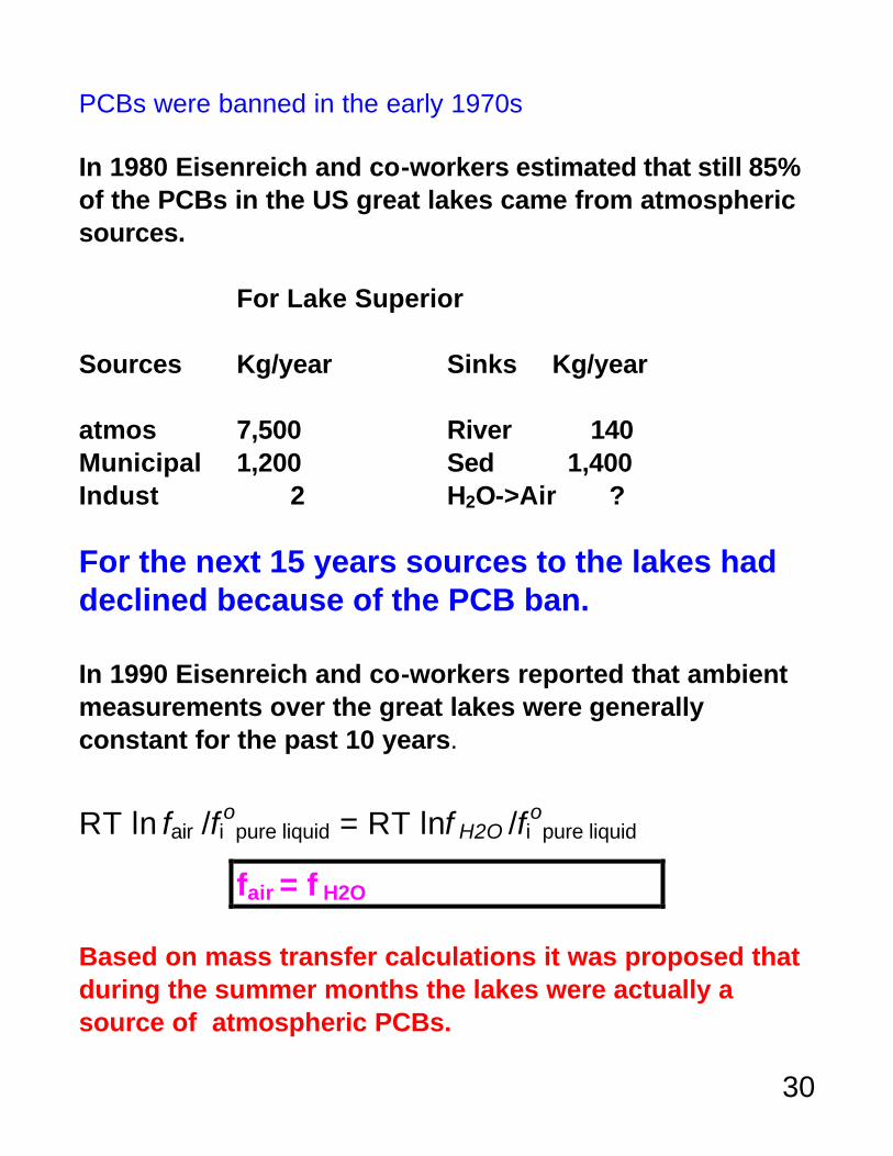
PCBs were banned in the early 1970s In 1980 Eisenreich and co-workers estimated that still 85% of the PCBs in the US great lakes came from atmospheric sources. For Lake Superior Sources Kg/year Sinks Kg/year atmos 7,500 River 140 Municipal 1,200 Sed 1,400 Indust 2 H2O->Air ? For the next 15 years sources to the lakes had declined because of the PCB ban. In 1990 Eisenreich and co-workers reported that ambient measurements over the great lakes were generally constant for the past 10 years.

RT ln fair /fio

pure liquid = RT lnf H2O /fi

opure liquid

fair = f H2O

Based on mass transfer calculations it was proposed that during the summer months the lakes were actually a source of atmospheric PCBs.

31

Effects of Stirring(shallow streams) page 234 page 234 Fig 10.7 O’connor and Dobbins (1958) proposed a relationship of the renewal rate of the film surface with the velocity of water and water depth r ≅ µw/dw

32

r ≅ µw/dw

vw= (Dw rw)1/2 = (Dw µw/ dw)1/2 for a stream of 50 cm depth and a water velocity of 1m/sec and with a benzene contamination(Dw= 1.02x10-5 cm2/sec) vw= (1.02x10-5 x100/50)1/2= 4.5x10-3cm/sec

typically vw is greater than 5x10-4 cm/sec; so if we take this as a reference value and use a typical water diffusion coef., and estimate the importance of turbulence

This is done by asking at what critical velocity to depth ratio will vw be less than 5x10-4 cm/sec

5x10-4 cm/sec < (Dw µw/ dw)1/2

this means that if µw/ dw < 0.03 sec-1, va will be very low

33

Measurements of the vw from streams using tracers or from spills are generally with in a factor of 2 from predictions by vw= (Dw µw/ dw)1/2

page 236

page 236, Figure 10.8

Schwartzenbach suggests vw(O2) = 4 x10-4+ 4x10-5µ2

10

from vw(O2) we can estimate vw(i) = vw(O2) {Dw(i) /Dw(O2)}

β

lab data β = 0.57 and α = 0.67

34

Total Transfer Velocity 1/vtot= 1/vw+ 1/(vaK’H) 1/vtot= 1/vw+ 1/(va

’) where va

’= vaK’H = vaKH/RT If we call the inverse transfer velocities layered resistances, a resistance ratio would measure the importance of the air film resistance to the water film resistance if Ra/w < 0.1 mass transfer is controlled by the water film Ra/w > 10 mass transfer is controlled by the air film in water vw(i) = vw(O2) {Dw(i) /Dw(O2)}

0.57

35

in air va(i) = va(H2O) {Da(i) /Da(H2O)}0.67

we can calculate va(O2) from vw(O2) = 4 x10-4+ 4x10-5µ2

10

va(H2O) from

Va(H2O) ~ 0.2 µ10(m/sec)+0.3 wind speed measured at one level can be translated to µ10 Diffusion coef Dw= 2.3x10-4/ V0.71

Dw= 2.35/ V0.73

36

Table 10.3 page 238

37

Transfer velocities vs. Henry’s law values

page 240, Figure 10.9

38

Surface Films Oily layers (amphiphilic or surface active) How do they alter the exchange of volatile chemicals through an air water boundary?

1.. Create another layer through with diffusion must take place. 2. dampen mixing and turbulence -lengthens diffusion distances and slows renewal rate page 252 Figure 10.13

39

air oil water Fluxtotal=fluxwater boundary= fluxoil boundary =fluxair boundary flux = velocity x ∆conc vw(Cw-Cw/o) = vw(Co/w-Co/a) = va(Ca/w-Ca) At the interface we previously assumed that Henry’s law was operating Ka/o= Ca/Co Co= conci in oil Ko/w= Co/Co

Ca/Cw= Ka/o Ko/w =K’H

Fluxtotal = Fluxtotal =

40

for O2 , K

’H is high an we can neglect 1/ (K’

H va ) for organics Ko/w is probably high page 253 Figure 10.14 `

41

Rate constants and fluxes If we look at the flux coming off a water surface, it has the units of flux = moles/(cm2 sec) depth conci if we divide the flux by the conci (moles/cm3)xdepth(cm) we come up with 1/sec, which is really the rate constant in rate of loss of conci from the entire body of water dconci/dt = -krate x concI

If the conc = Cw

dCw/dt = flux/(Cw x depth) x Cw = flux/depth dCw/dt = flux/depth = -krate x Cw

flux x surface/volume = -krate x Cw