Embed Size (px)
Citation preview
393
C H A P T E R
SINUSOIDAL STEADY-STATE ANALYSIS
1 0
An expert problem solver must be endowed with two incompatible quan-tities, a restless imagination and a patient pertinacity.
—Howard W. Eves
Enhancing Your CareerCareer in Software Engineering Software engineering isthat aspect of engineering that deals with the practical ap-plication of scientific knowledge in the design, construction,and validation of computer programs and the associated doc-umentation required to develop, operate, and maintain them.It is a branch of electrical engineering that is becoming in-creasingly important as more and more disciplines requireone form of software package or another to perform rou-tine tasks and as programmable microelectronic systems areused in more and more applications.
The role of a software engineer should not be con-fused with that of a computer scientist; the software engi-neer is a practitioner, not a theoretician. A software engineershould have good computer-programming skill and be famil-iar with programming languages, in particular C++, whichis becoming increasingly popular. Because hardware andsoftware are closely interlinked, it is essential that a soft-ware engineer have a thorough understanding of hardwaredesign. Most important, the software engineer should havesome specialized knowledge of the area in which the soft-ware development skill is to be applied.
All in all, the field of software engineering offersa great career to those who enjoy programming and devel-oping software packages. The higher rewards will go tothose having the best preparation, with the most interestingand challenging opportunities going to those with graduateeducation.
Output of a modeling software.(Courtesy of National Instruments.)
394 PART 2 AC Circuits
10.1 INTRODUCTIONIn Chapter 9, we learned that the forced or steady-state response of cir-cuits to sinusoidal inputs can be obtained by using phasors. We also knowthat Ohm’s and Kirchhoff’s laws are applicable to ac circuits. In thischapter, we want to see how nodal analysis, mesh analysis, Thevenin’stheorem, Norton’s theorem, superposition, and source transformationsare applied in analyzing ac circuits. Since these techniques were alreadyintroduced for dc circuits, our major effort here will be to illustrate withexamples.
Analyzing ac circuits usually requires three steps.
S t e p s t o A n a l y z e a c C i r c u i t s :1. Transform the circuit to the phasor or frequency domain.
2. Solve the problem using circuit techniques (nodal analysis, meshanalysis, superposition, etc.).
3. Transform the resulting phasor to the time domain.
Step 1 is not necessary if the problem is specified in the frequency domain.In step 2, the analysis is performed in the same manner as dc circuitanalysis except that complex numbers are involved. Having read Chapter9, we are adept at handling step 3.Frequency-domain analysis of an ac circuit via
phasors is much easier than analysis of the cir-cuit in the time domain.
Toward the end of the chapter, we learn how to applyPSpice insolving ac circuit problems. We finally apply ac circuit analysis to twopractical ac circuits: oscillators and ac transistor circuits.
10.2 NODAL ANALYSISThe basis of nodal analysis is Kirchhoff’s current law. Since KCL is validfor phasors, as demonstrated in Section 9.6, we can analyze ac circuitsby nodal analysis. The following examples illustrate this.
E X A M P L E 1 0 . 1
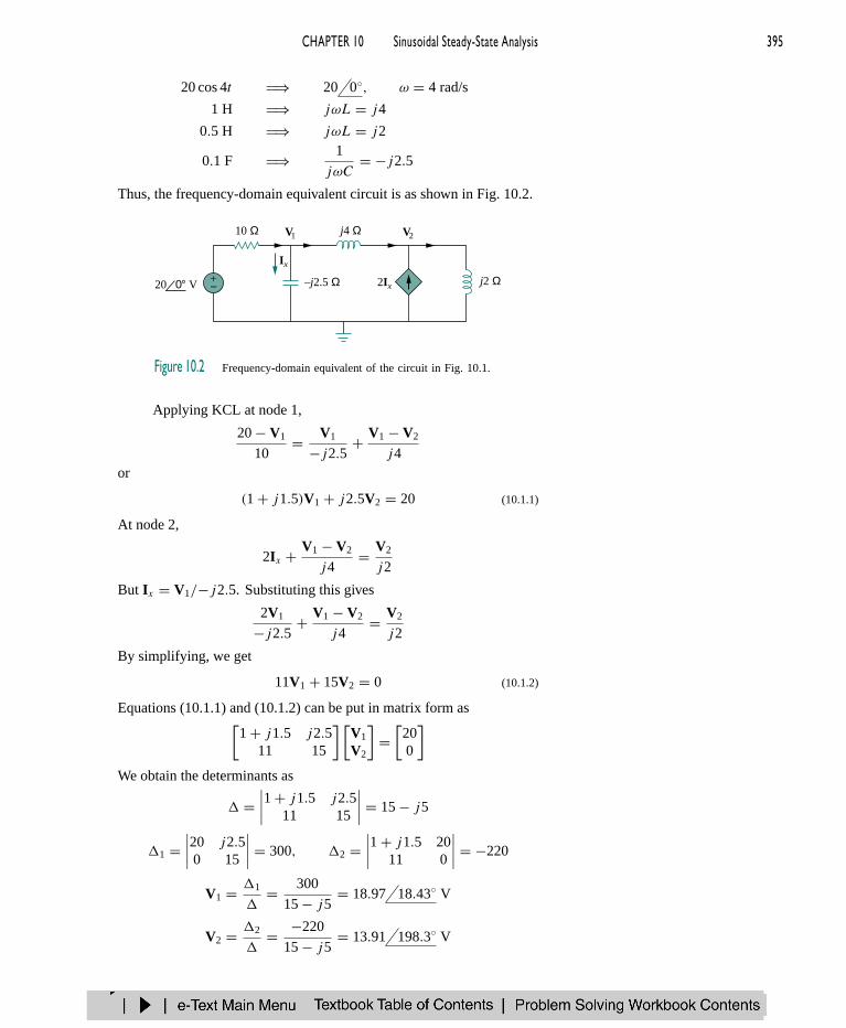
Find ix in the circuit of Fig. 10.1 using nodal analysis.
0.5 H0.1 F
1 H10 Ω
2ix
ix
+−20 cos 4t V
Figure 10.1 For Example 10.1.
Solution:
We first convert the circuit to the frequency domain:
CHAPTER 10 Sinusoidal Steady-State Analysis 395
20 cos 4t ⇒ 20 0, ω = 4 rad/s
1 H ⇒ jωL = j4
0.5 H ⇒ jωL = j2
0.1 F ⇒ 1
jωC= −j2.5
Thus, the frequency-domain equivalent circuit is as shown in Fig. 10.2.
–j2.5 Ω j2 Ω
j4 Ω10 Ω
2Ix
Ix
+−
V1 V2
20 0° V
Figure 10.2 Frequency-domain equivalent of the circuit in Fig. 10.1.
Applying KCL at node 1,
20 − V1
10= V1
−j2.5+ V1 − V2
j4or
(1 + j1.5)V1 + j2.5V2 = 20 (10.1.1)
At node 2,
2Ix + V1 − V2
j4= V2
j2
But Ix = V1/−j2.5. Substituting this gives
2V1
−j2.5+ V1 − V2
j4= V2
j2
By simplifying, we get
11V1 + 15V2 = 0 (10.1.2)
Equations (10.1.1) and (10.1.2) can be put in matrix form as[1 + j1.5 j2.5
11 15
] [V1
V2
]=[
200
]We obtain the determinants as
=∣∣∣∣1 + j1.5 j2.5
11 15
∣∣∣∣ = 15 − j5
1 =∣∣∣∣20 j2.5
0 15
∣∣∣∣ = 300, 2 =∣∣∣∣1 + j1.5 20
11 0
∣∣∣∣ = −220
V1 = 1
= 300
15 − j5= 18.97 18.43 V
V2 = 2
= −220
15 − j5= 13.91 198.3 V
396 PART 2 AC Circuits
The current Ix is given by
Ix = V1
−j2.5= 18.97 18.43
2.5 − 90= 7.59 108.4 A
Transforming this to the time domain,
ix = 7.59 cos(4t + 108.4) A
P R A C T I C E P R O B L E M 1 0 . 1
Using nodal analysis, find v1 and v2 in the circuit of Fig. 10.3.
4 Ω
2 Ω 3vxvx 2 H
0.2 Fv1 v2
+−
+
−10 sin 2t A
Figure 10.3 For Practice Prob. 10.1.
Answer: v1(t) = 20.96 sin(2t + 58) V,v2(t) = 44.11 sin(2t + 41) V.
E X A M P L E 1 0 . 2
Compute V1 and V2 in the circuit of Fig. 10.4.
4 Ω
12 Ω
1 2V1 V2
–j3 Ω j6 Ω
+ −10 45° V
3 0° A
Figure 10.4 For Example 10.2.
Solution:
Nodes 1 and 2 form a supernode as shown in Fig. 10.5. Applying KCLat the supernode gives
3 = V1
−j3+ V2
j6+ V2
12or
36 = j4V1 + (1 − j2)V2 (10.2.1)
But a voltage source is connected between nodes 1 and 2, so that
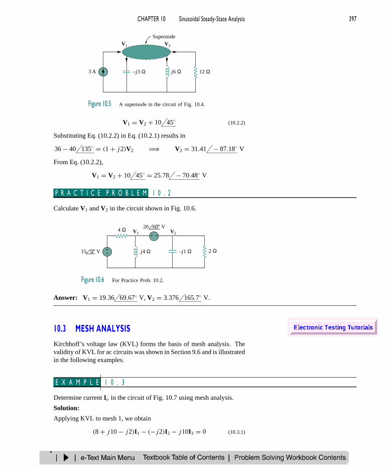
CHAPTER 10 Sinusoidal Steady-State Analysis 397
–j3 Ω j6 Ω 12 Ω3 A
SupernodeV1 V2
Figure 10.5 A supernode in the circuit of Fig. 10.4.
V1 = V2 + 10 45 (10.2.2)
Substituting Eq. (10.2.2) in Eq. (10.2.1) results in
36 − 40 135 = (1 + j2)V2 ⇒ V2 = 31.41 − 87.18 V
From Eq. (10.2.2),
V1 = V2 + 10 45 = 25.78 − 70.48 V
P R A C T I C E P R O B L E M 1 0 . 2
Calculate V1 and V2 in the circuit shown in Fig. 10.6.
4 Ω
2 Ωj4 Ω –j1 Ω
+ −
+−
V1 V2
15 0° V
20 60° V
Figure 10.6 For Practice Prob. 10.2.
Answer: V1 = 19.36 69.67 V, V2 = 3.376 165.7 V.
10.3 MESH ANALYSISKirchhoff’s voltage law (KVL) forms the basis of mesh analysis. Thevalidity of KVL for ac circuits was shown in Section 9.6 and is illustratedin the following examples.
E X A M P L E 1 0 . 3
Determine current Io in the circuit of Fig. 10.7 using mesh analysis.
Solution:
Applying KVL to mesh 1, we obtain
(8 + j10 − j2)I1 − (−j2)I2 − j10I3 = 0 (10.3.1)

398 PART 2 AC Circuits
4 Ω
8 Ω –j2 Ω
–j2 Ω
j10 Ω+−
Io
I2
I3
I1
5 0° A
20 90° V
Figure 10.7 For Example 10.3.
For mesh 2,
(4 − j2 − j2)I2 − (−j2)I1 − (−j2)I3 + 20 90 = 0 (10.3.2)
For mesh 3, I3 = 5. Substituting this in Eqs. (10.3.1) and (10.3.2), weget
(8 + j8)I1 + j2I2 = j50 (10.3.3)
j2I1 + (4 − j4)I2 = −j20 − j10 (10.3.4)
Equations (10.3.3) and (10.3.4) can be put in matrix form as[8 + j8 j2j2 4 − j4
] [I1
I2
]=[j50
−j30
]
from which we obtain the determinants
=∣∣∣∣8 + j8 j2
j2 4 − j4
∣∣∣∣ = 32(1 + j)(1 − j) + 4 = 68
2 =∣∣∣∣8 + j8 j50
j2 −j30
∣∣∣∣ = 340 − j240 = 416.17 − 35.22
I2 = 2
= 416.17 − 35.22
68= 6.12 − 35.22 A
The desired current is
Io = −I2 = 6.12 144.78 A
P R A C T I C E P R O B L E M 1 0 . 3
Find Io in Fig. 10.8 using mesh analysis.
8 Ωj4 Ω
–j2 Ω 6 Ω
+−
Io
2 0° A
10 30° V
Figure 10.8 For Practice Prob. 10.3.
Answer: 1.194 65.45 A.

CHAPTER 10 Sinusoidal Steady-State Analysis 399
E X A M P L E 1 0 . 4
Solve for Vo in the circuit in Fig. 10.9 using mesh analysis.
8 Ω
6 Ω
–j2 Ω
–j4 Ωj5 Ω
4 0˚ A
+− Vo
+
−3 0° A10 0° V
Figure 10.9 For Example 10.4.
Solution:
As shown in Fig. 10.10, meshes 3 and 4 form a supermesh due to thecurrent source between the meshes. For mesh 1, KVL gives
−10 + (8 − j2)I1 − (−j2)I2 − 8I3 = 0
or
(8 − j2)I1 + j2I2 − 8I3 = 10 (10.4.1)
For mesh 2,
I2 = −3 (10.4.2)
For the supermesh,
(8 − j4)I3 − 8I1 + (6 + j5)I4 − j5I2 = 0 (10.4.3)
Due to the current source between meshes 3 and 4, at node A,
I4 = I3 + 4 (10.4.4)
Combining Eqs. (10.4.1) and (10.4.2),
(8 − j2)I1 − 8I3 = 10 + j6 (10.4.5)
Combining Eqs. (10.4.2) to (10.4.4),
−8I1 + (14 + j)I3 = −24 − j35 (10.4.6)
8 Ω
6 Ω
–j2 Ω
–j4 Ω
j5 Ω
10 V 3 A
4 A
A
+−
+
− I2
I3
I3 I4
I4
I1
Supermesh
Vo
Figure 10.10 Analysis of the circuit in Fig. 10.9.

400 PART 2 AC Circuits
From Eqs. (10.4.5) and (10.4.6), we obtain the matrix equation[8 − j2 −8
−8 14 + j
] [I1
I3
]=[
10 + j6−24 − j35
]
We obtain the following determinants
=∣∣∣∣8 − j2 −8
−8 14 + j
∣∣∣∣ = 112 + j8 − j28 + 2 − 64 = 50 − j20
1 =∣∣∣∣ 10 + j6 −8−24 − j35 14 + j
∣∣∣∣ = 140 + j10 + j84 − 6 − 192 − j280
= −58 − j186
Current I1 is obtained as
I1 = 1
= −58 − j186
50 − j20= 3.618 274.5 A
The required voltage Vo is
Vo = −j2(I1 − I2) = −j2(3.618 274.5 + 3)
= −7.2134 − j6.568 = 9.756 222.32 V
P R A C T I C E P R O B L E M 1 0 . 4
Calculate current Io in the circuit of Fig. 10.11.
j8 Ω
–j6 Ω
–j4 Ω
5 Ω
10 Ω Io
+−50 0° V
2 0° A
Figure 10.11 For Practice Prob. 10.4.
Answer: 5.075 5.943 A.
10.4 SUPERPOSITION THEOREMSince ac circuits are linear, the superposition theorem applies to ac circuitsthe same way it applies to dc circuits. The theorem becomes importantif the circuit has sources operating at different frequencies. In this case,since the impedances depend on frequency, we must have a differentfrequency-domain circuit for each frequency. The total response mustbe obtained by adding the individual responses in the time domain. It isincorrect to try to add the responses in the phasor or frequency domain.Why? Because the exponential factor ejωt is implicit in sinusoidal analy-sis, and that factor would change for every angular frequency ω. It wouldtherefore not make sense to add responses at different frequencies in thephasor domain. Thus, when a circuit has sources operating at different
CHAPTER 10 Sinusoidal Steady-State Analysis 401
frequencies, one must add the responses due to the individual frequenciesin the time domain.
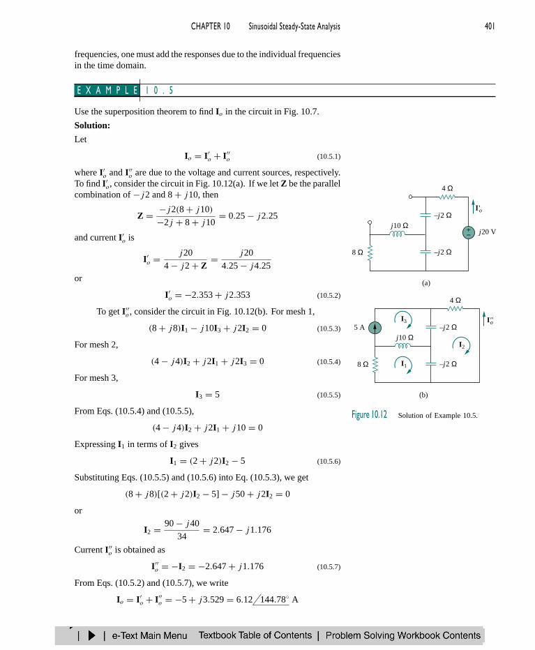
E X A M P L E 1 0 . 5
Use the superposition theorem to find Io in the circuit in Fig. 10.7.
Solution:
Let
Io = I′o + I′′
o (10.5.1)
where I′o and I′′
o are due to the voltage and current sources, respectively.To find I′
o, consider the circuit in Fig. 10.12(a). If we let Z be the parallelcombination of −j2 and 8 + j10, then
Z = −j2(8 + j10)
−2j + 8 + j10= 0.25 − j2.25
and current I′o is
I′o = j20
4 − j2 + Z= j20
4.25 − j4.25or
I′o = −2.353 + j2.353 (10.5.2)
4 Ω
8 Ω –j2 Ω
–j2 Ωj10 Ω
j20 V+−
I'o
(a)
(b)
4 Ω
8 Ω –j2 Ω
–j2 Ωj10 Ω
5 AI''o
I2
I3
I1
Figure 10.12 Solution of Example 10.5.
To get I′′o , consider the circuit in Fig. 10.12(b). For mesh 1,
(8 + j8)I1 − j10I3 + j2I2 = 0 (10.5.3)
For mesh 2,
(4 − j4)I2 + j2I1 + j2I3 = 0 (10.5.4)
For mesh 3,
I3 = 5 (10.5.5)
From Eqs. (10.5.4) and (10.5.5),
(4 − j4)I2 + j2I1 + j10 = 0
Expressing I1 in terms of I2 gives
I1 = (2 + j2)I2 − 5 (10.5.6)
Substituting Eqs. (10.5.5) and (10.5.6) into Eq. (10.5.3), we get
(8 + j8)[(2 + j2)I2 − 5] − j50 + j2I2 = 0
or
I2 = 90 − j40
34= 2.647 − j1.176
Current I′′o is obtained as
I′′o = −I2 = −2.647 + j1.176 (10.5.7)
From Eqs. (10.5.2) and (10.5.7), we write
Io = I′o + I′′
o = −5 + j3.529 = 6.12 144.78 A
402 PART 2 AC Circuits
which agrees with what we got in Example 10.3. It should be notedthat applying the superposition theorem is not the best way to solve thisproblem. It seems that we have made the problem twice as hard asthe original one by using superposition. However, in Example 10.6,superposition is clearly the easiest approach.
P R A C T I C E P R O B L E M 1 0 . 5
Find current Io in the circuit of Fig. 10.8 using the superposition theorem.
Answer: 1.194 65.45 A.
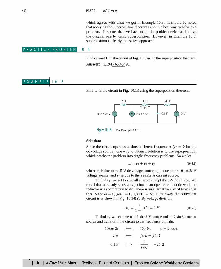
E X A M P L E 1 0 . 6
Find vo in the circuit in Fig. 10.13 using the superposition theorem.
2 H 1 Ω 4 Ω
0.1 F 5 V+−
+−10 cos 2t V 2 sin 5t A
−+ vo
Figure 10.13 For Example 10.6.
Solution:
Since the circuit operates at three different frequencies (ω = 0 for thedc voltage source), one way to obtain a solution is to use superposition,which breaks the problem into single-frequency problems. So we let
vo = v1 + v2 + v3 (10.6.1)
where v1 is due to the 5-V dc voltage source, v2 is due to the 10 cos 2t Vvoltage source, and v3 is due to the 2 sin 5t A current source.
To find v1, we set to zero all sources except the 5-V dc source. Werecall that at steady state, a capacitor is an open circuit to dc while aninductor is a short circuit to dc. There is an alternative way of looking atthis. Since ω = 0, jωL = 0, 1/jωC = ∞. Either way, the equivalentcircuit is as shown in Fig. 10.14(a). By voltage division,
−v1 = 1
1 + 4(5) = 1 V (10.6.2)
To find v2, we set to zero both the 5-V source and the 2 sin 5t currentsource and transform the circuit to the frequency domain.
10 cos 2t ⇒ 10 0, ω = 2 rad/s
2 H ⇒ jωL = j4
0.1 F ⇒ 1
jωC= −j5
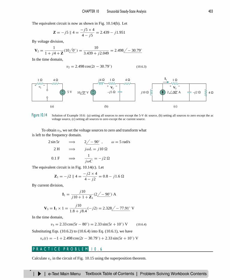
CHAPTER 10 Sinusoidal Steady-State Analysis 403
The equivalent circuit is now as shown in Fig. 10.14(b). Let
Z = −j5 ‖ 4 = −j5 × 4
4 − j5= 2.439 − j1.951
By voltage division,
V2 = 1
1 + j4 + Z(10 0 ) = 10
3.439 + j2.049= 2.498 − 30.79
In the time domain,
v2 = 2.498 cos(2t − 30.79) (10.6.3)
1 Ω 4 Ω
5 V+−
−+ v1
(a) (b) (c)
1 Ωj4 Ω
–j5 Ω
4 Ω
+−
1 Ω
4 Ω–j2 Ωj10 Ω
I1
10 0° V 2 –90° A
+ −V2+ −V3
Figure 10.14 Solution of Example 10.6: (a) setting all sources to zero except the 5-V dc source, (b) setting all sources to zero except the acvoltage source, (c) setting all sources to zero except the ac current source.
To obtain v3, we set the voltage sources to zero and transform whatis left to the frequency domain.
2 sin 5t ⇒ 2 − 90 , ω = 5 rad/s
2 H ⇒ jωL = j10
0.1 F ⇒ 1
jωC= −j2
The equivalent circuit is in Fig. 10.14(c). Let
Z1 = −j2 ‖ 4 = −j2 × 4
4 − j2= 0.8 − j1.6
By current division,
I1 = j10
j10 + 1 + Z1(2 − 90) A
V3 = I1 × 1 = j10
1.8 + j8.4(−j2) = 2.328 − 77.91 V
In the time domain,
v3 = 2.33 cos(5t − 80) = 2.33 sin(5t + 10) V (10.6.4)
Substituting Eqs. (10.6.2) to (10.6.4) into Eq. (10.6.1), we have
vo(t) = −1 + 2.498 cos(2t − 30.79) + 2.33 sin(5t + 10) V
P R A C T I C E P R O B L E M 1 0 . 6
Calculate vo in the circuit of Fig. 10.15 using the superposition theorem.

404 PART 2 AC Circuits
8 Ω
0.2 F 1 H+−30 sin 5t V 2 cos 10t A
+
−vo
Figure 10.15 For Practice Prob. 10.6.
Answer: 4.631 sin(5t − 81.12) + 1.051 cos(10t − 86.24) V.
10.5 SOURCE TRANSFORMATIONAs Fig. 10.16 shows, source transformation in the frequency domaininvolves transforming a voltage source in series with an impedance to acurrent source in parallel with an impedance, or vice versa. As we gofrom one source type to another, we must keep the following relationshipin mind:
Vs = ZsIs ⇐⇒ Is = Vs
Zs
(10.1)
a
b
Vs
Vs = ZsIs
Z s
Z s+−
a
b
Is
Is = Zs
Vs
Figure 10.16 Source transformation.
E X A M P L E 1 0 . 7
Calculate Vx in the circuit of Fig. 10.17 using the method of source trans-formation.
5 Ω
j4 Ω
–j13 Ω
3 Ω
10 Ω
4 Ω
+−
+
−Vx2 0 –90° V
Figure 10.17 For Example 10.7.
CHAPTER 10 Sinusoidal Steady-State Analysis 405
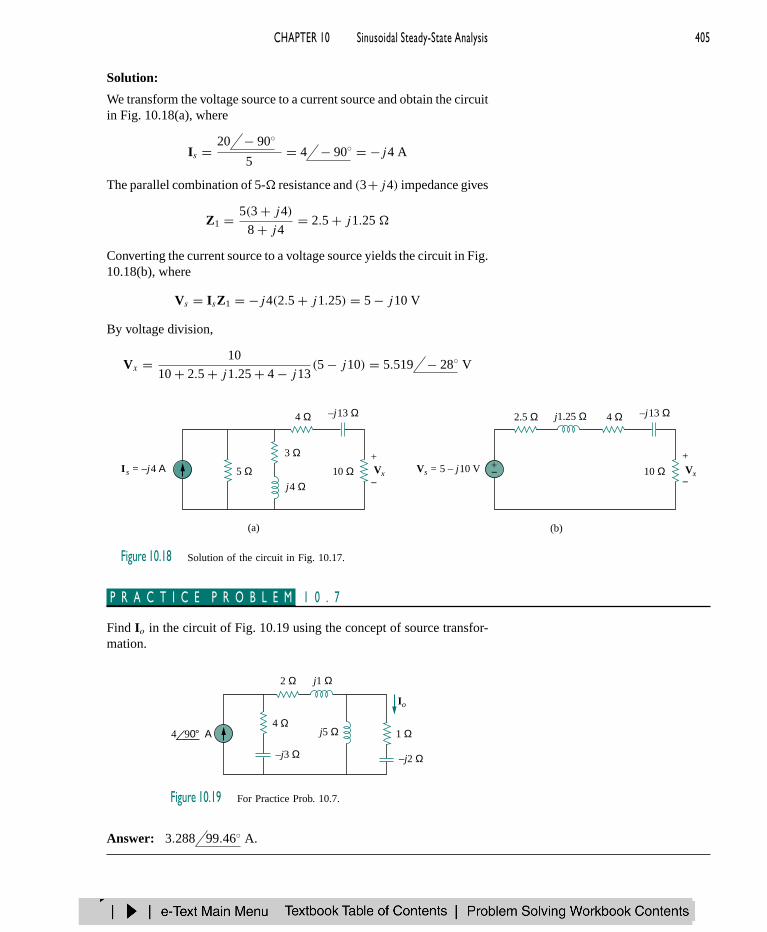
Solution:
We transform the voltage source to a current source and obtain the circuitin Fig. 10.18(a), where
Is = 20 − 90
5= 4 − 90 = −j4 A
The parallel combination of 5- resistance and (3+j4) impedance gives
Z1 = 5(3 + j4)
8 + j4= 2.5 + j1.25
Converting the current source to a voltage source yields the circuit in Fig.10.18(b), where
Vs = IsZ1 = −j4(2.5 + j1.25) = 5 − j10 V
By voltage division,
Vx = 10
10 + 2.5 + j1.25 + 4 − j13(5 − j10) = 5.519 − 28 V
5 Ωj4 Ω
–j13 Ω
3 Ω
10 Ω
4 Ω
+
−
+
−V xIs = –j4 Α
–j13 Ω
10 Ω
4 Ω2.5 Ω j1.25 Ω
VxVs = 5 – j10 V +−
(a) (b)
Figure 10.18 Solution of the circuit in Fig. 10.17.
P R A C T I C E P R O B L E M 1 0 . 7
Find Io in the circuit of Fig. 10.19 using the concept of source transfor-mation.
–j3 Ω
j5 Ω
j1 Ω2 Ω
Io
–j2 Ω
4 90° Α4 Ω
1 Ω
Figure 10.19 For Practice Prob. 10.7.
Answer: 3.288 99.46 A.

406 PART 2 AC Circuits
10.6 THEVENIN AND NORTON EQUIVALENT CIRCUITSThevenin’s and Norton’s theorems are applied to ac circuits in the sameway as they are to dc circuits. The only additional effort arises from theneed to manipulate complex numbers. The frequency-domain version ofa Thevenin equivalent circuit is depicted in Fig. 10.20, where a linearcircuit is replaced by a voltage source in series with an impedance. TheNorton equivalent circuit is illustrated in Fig. 10.21, where a linear circuitis replaced by a current source in parallel with an impedance. Keep inmind that the two equivalent circuits are related as
VTh = ZN IN, ZTh = ZN (10.2)
just as in source transformation. VTh is the open-circuit voltage while INis the short-circuit current.
a
b
ZTh
a
b
VThLinearcircuit
+−
Figure 10.20 Thevenin equivalent.
a
b
ZN
a
b
IN
Linearcircuit
Figure 10.21 Norton equivalent.
If the circuit has sources operating at different frequencies (seeExample 10.6, for example), the Thevenin or Norton equivalent circuitmust be determined at each frequency. This leads to entirely differentequivalent circuits, one for each frequency, not one equivalent circuitwith equivalent sources and equivalent impedances.
E X A M P L E 1 0 . 8
Obtain the Thevenin equivalent at terminalsa-b of the circuit in Fig. 10.22.
4 Ω
d
a b
f
ce
–j6 Ω
j12 Ω8 Ω
+− a b120 75° V
Figure 10.22 For Example 10.8.
Solution:
We find ZTh by setting the voltage source to zero. As shown in Fig.10.23(a), the 8- resistance is now in parallel with the −j6 reactance, sothat their combination gives
Z1 = −j6 ‖ 8 = −j6 × 8
8 − j6= 2.88 − j3.84
Similarly, the 4- resistance is in parallel with the j12 reactance, andtheir combination gives
Z2 = 4 ‖ j12 = j12 × 4
4 + j12= 3.6 + j1.2
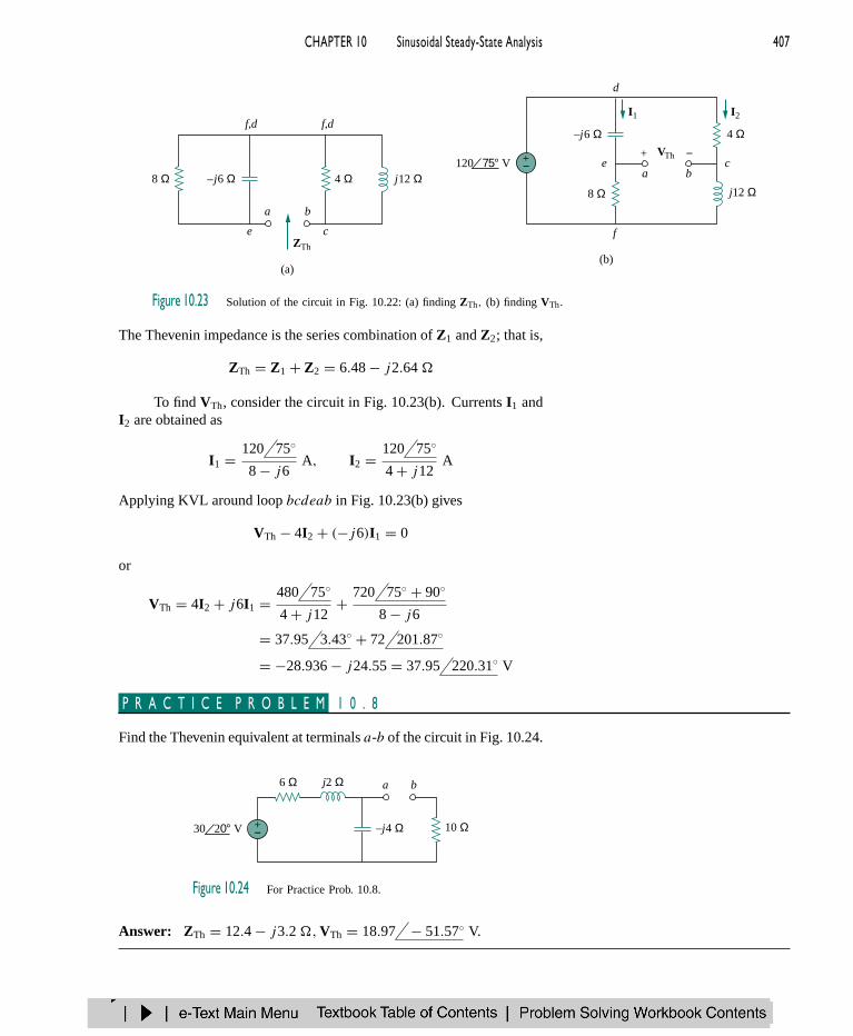
CHAPTER 10 Sinusoidal Steady-State Analysis 407
4 Ω8 Ω –j6 Ω j12 Ω
ZTh
VTh
a
e c
f,d f,d
b
(a)(b)
8 Ω
4 Ω
j12 Ω
–j6 Ω
+−
I2I1
d
ea b
c
f
−+120 75° V
Figure 10.23 Solution of the circuit in Fig. 10.22: (a) finding ZTh, (b) finding VTh.
The Thevenin impedance is the series combination of Z1 and Z2; that is,
ZTh = Z1 + Z2 = 6.48 − j2.64
To find VTh, consider the circuit in Fig. 10.23(b). Currents I1 andI2 are obtained as
I1 = 120 75
8 − j6A, I2 = 120 75
4 + j12A
Applying KVL around loop bcdeab in Fig. 10.23(b) gives
VTh − 4I2 + (−j6)I1 = 0
or
VTh = 4I2 + j6I1 = 480 75
4 + j12+ 720 75 + 90
8 − j6
= 37.95 3.43 + 72 201.87
= −28.936 − j24.55 = 37.95 220.31 V
P R A C T I C E P R O B L E M 1 0 . 8
Find the Thevenin equivalent at terminals a-b of the circuit in Fig. 10.24.
–j4 Ω
j2 Ω6 Ω
10 Ω+−
a b
30 20° V
Figure 10.24 For Practice Prob. 10.8.
Answer: ZTh = 12.4 − j3.2 ,VTh = 18.97 − 51.57 V.
408 PART 2 AC Circuits
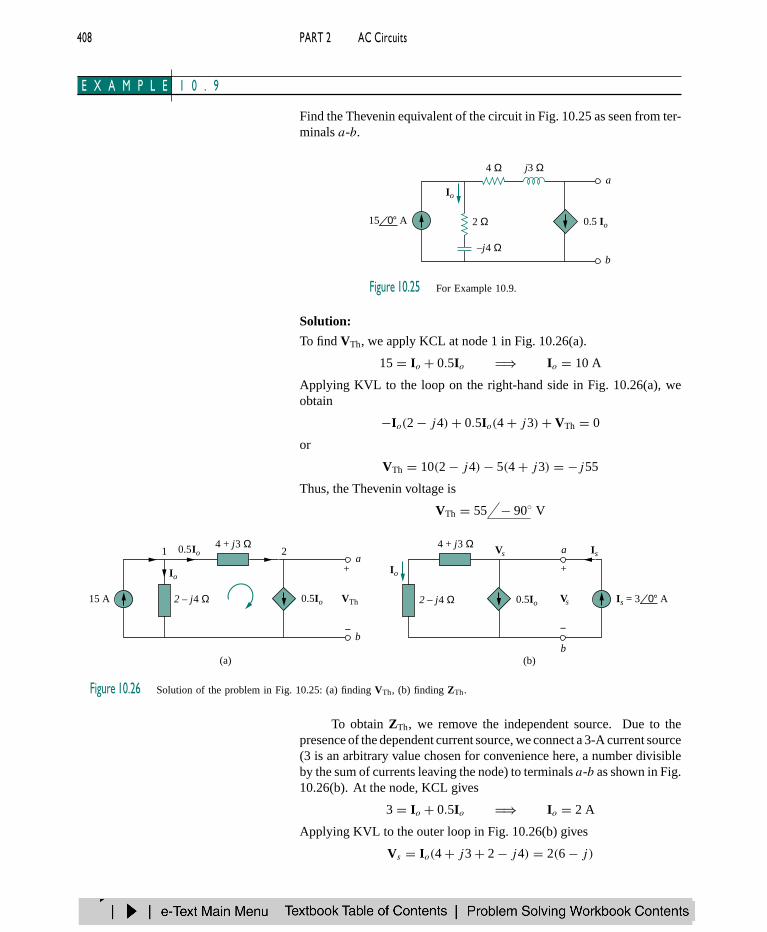
E X A M P L E 1 0 . 9
Find the Thevenin equivalent of the circuit in Fig. 10.25 as seen from ter-minals a-b.
–j4 Ω
j3 Ω4 Ω
2 Ω
a
b
Io
0.5 Io15 0° A
Figure 10.25 For Example 10.9.
Solution:
To find VTh, we apply KCL at node 1 in Fig. 10.26(a).
15 = Io + 0.5Io ⇒ Io = 10 A
Applying KVL to the loop on the right-hand side in Fig. 10.26(a), weobtain
−Io(2 − j4) + 0.5Io(4 + j3) + VTh = 0
or
VTh = 10(2 − j4) − 5(4 + j3) = −j55
Thus, the Thevenin voltage is
VTh = 55 − 90 V
4 + j3 Ω
2 – j4 Ω
a
b
Io
0.5Io
0.5Io VTh15 A
+
−
214 + j3 Ω
2 – j4 Ω
a
b
Vs Is
0.5Io
Io
Is = 3 0° A
(a) (b)
+
−
Vs
Figure 10.26 Solution of the problem in Fig. 10.25: (a) finding VTh, (b) finding ZTh.
To obtain ZTh, we remove the independent source. Due to thepresence of the dependent current source, we connect a 3-A current source(3 is an arbitrary value chosen for convenience here, a number divisibleby the sum of currents leaving the node) to terminals a-b as shown in Fig.10.26(b). At the node, KCL gives
3 = Io + 0.5Io ⇒ Io = 2 A
Applying KVL to the outer loop in Fig. 10.26(b) gives
Vs = Io(4 + j3 + 2 − j4) = 2(6 − j)
CHAPTER 10 Sinusoidal Steady-State Analysis 409
The Thevenin impedance is
ZTh = Vs
Is= 2(6 − j)
3= 4 − j0.6667
P R A C T I C E P R O B L E M 1 0 . 9
Determine the Thevenin equivalent of the circuit in Fig. 10.27 as seen fromthe terminals a-b.
–j2 Ω
j4 Ω8 Ω
4 Ω
a
b
0.2Vo5 0° A
−+ Vo
Figure 10.27 For Practice Prob. 10.9.
Answer: ZTh = 12.166 136.3 ,VTh = 7.35 72.9 V.
E X A M P L E 1 0 . 1 0
Obtain current Io in Fig. 10.28 using Norton’s theorem.
3 0° A
40 90° V
8 Ω5 Ω
20 Ω
10 Ω
–j2 Ω
j4 Ωj15 Ω+
−
Io
a
b
Figure 10.28 For Example 10.10.
Solution:
Our first objective is to find the Norton equivalent at terminals a-b. ZN
is found in the same way as ZTh. We set the sources to zero as shownin Fig. 10.29(a). As evident from the figure, the (8 − j2) and (10 + j4)impedances are short-circuited, so that
ZN = 5
To get IN , we short-circuit terminals a-b as in Fig. 10.29(b) andapply mesh analysis. Notice that meshes 2 and 3 form a supermeshbecause of the current source linking them. For mesh 1,
−j40 + (18 + j2)I1 − (8 − j2)I2 − (10 + j4)I3 = 0 (10.10.1)
For the supermesh,
(13 − j2)I2 + (10 + j4)I3 − (18 + j2)I1 = 0 (10.10.2)
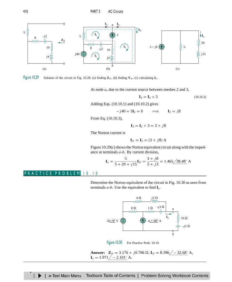
410 PART 2 AC Circuits
3
8
5
10–j2
j4j40 +
−
IN
I3
I2
I3I2
I1
a
b(b)
520
j15
3 + j8
Io
(c)
8
5
10
–j2
j4
ZN
(a)
Figure 10.29 Solution of the circuit in Fig. 10.28: (a) finding ZN , (b) finding VN , (c) calculating Io.
At node a, due to the current source between meshes 2 and 3,
I3 = I2 + 3 (10.10.3)
Adding Eqs. (10.10.1) and (10.10.2) gives
−j40 + 5I2 = 0 ⇒ I2 = j8
From Eq. (10.10.3),
I3 = I2 + 3 = 3 + j8
The Norton current is
IN = I3 = (3 + j8) A
Figure 10.29(c) shows the Norton equivalent circuit along with the imped-ance at terminals a-b. By current division,
Io = 5
5 + 20 + j15IN = 3 + j8
5 + j3= 1.465 38.48 A
P R A C T I C E P R O B L E M 1 0 . 1 0
Determine the Norton equivalent of the circuit in Fig. 10.30 as seen fromterminals a-b. Use the equivalent to find Io.
j2 Ω
a
b
Io
–j3 Ω
–j5 Ω
+−
8 Ω
4 Ω
1 Ω
10 Ω20 0° V 4 –90° A
Figure 10.30 For Practice Prob. 10.10.
Answer: ZN = 3.176 + j0.706 , IN = 8.396 − 32.68 A,Io = 1.971 − 2.101 A.
CHAPTER 10 Sinusoidal Steady-State Analysis 411
10.7 OP AMP AC CIRCUITSThe three steps stated in Section 10.1 also apply to op amp circuits, aslong as the op amp is operating in the linear region. As usual, we willassume ideal op amps. (See Section 5.2.) As discussed in Chapter 5, thekey to analyzing op amp circuits is to keep two important properties ofan ideal op amp in mind:
1. No current enters either of its input terminals.
2. The voltage across its input terminals is zero.
The following examples will illustrate these ideas.
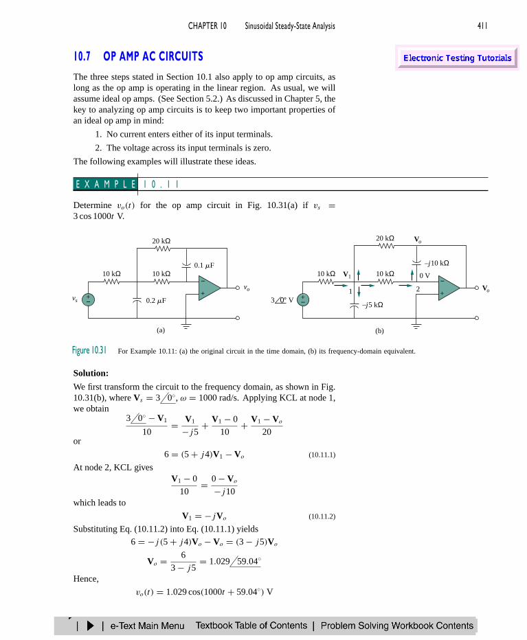
E X A M P L E 1 0 . 1 1
Determine vo(t) for the op amp circuit in Fig. 10.31(a) if vs =3 cos 1000t V.
+
−
+−
Vo
Vo
V1
–j5 kΩ
–j10 kΩ10 kΩ 10 kΩ
20 kΩ
3 0° V +
−
+−vs
vo
10 kΩ 10 kΩ0.1 mF
0.2 mF
20 kΩ
1 2
0 V
(a) (b)
Figure 10.31 For Example 10.11: (a) the original circuit in the time domain, (b) its frequency-domain equivalent.
Solution:
We first transform the circuit to the frequency domain, as shown in Fig.10.31(b), where Vs = 3 0, ω = 1000 rad/s. Applying KCL at node 1,we obtain
3 0 − V1
10= V1
−j5+ V1 − 0
10+ V1 − Vo
20or
6 = (5 + j4)V1 − Vo (10.11.1)
At node 2, KCL givesV1 − 0
10= 0 − Vo
−j10which leads to
V1 = −jVo (10.11.2)
Substituting Eq. (10.11.2) into Eq. (10.11.1) yields
6 = −j (5 + j4)Vo − Vo = (3 − j5)Vo
Vo = 6
3 − j5= 1.029 59.04
Hence,
vo(t) = 1.029 cos(1000t + 59.04) V

412 PART 2 AC Circuits
P R A C T I C E P R O B L E M 1 0 . 1 1
Find vo and io in the op amp circuit of Fig. 10.32. Let vs =2 cos 5000t V.
+
−+−vs
vo
10 kΩ
20 kΩ
20 nF
10 nFio
Figure 10.32 For Practice Prob. 10.11.
Answer: 0.667 sin 5000t V, 66.67 sin 5000t µA.
E X A M P L E 1 0 . 1 2
Compute the closed-loop gain and phase shift for the circuit in Fig. 10.33.Assume that R1 = R2 = 10 k, C1 = 2 µF, C2 = 1 µF, and ω =200 rad/s.
+
−
+−vs vo
R1R2
C2
C1
+
−
Figure 10.33 For Example 10.12.
Solution:
The feedback and input impedances are calculated as
Zf = R2
∥∥∥∥ 1
jωC2= R2
1 + jωR2C2
Zi = R1 + 1
jωC1= 1 + jωR1C1
jωC1
Since the circuit in Fig. 10.33 is an inverting amplifier, the closed-loopgain is given by
G = Vo
Vs
= −Zf
Zi
= jωC1R2
(1 + jωR1C1)(1 + jωR2C2)
Substituting the given values of R1, R2, C1, C2, and ω, we obtain
G = j4
(1 + j4)(1 + j2)= 0.434 − 49.4
Thus the closed-loop gain is 0.434 and the phase shift is −49.4.
P R A C T I C E P R O B L E M 1 0 . 1 2
Obtain the closed-loop gain and phase shift for the circuit in Fig. 10.34.Let R = 10 k, C = 1 µF, and ω = 1000 rad/s.
+
−+−vs
vo
R R
C
Figure 10.34 For Practice Prob. 10.12.
Answer: 1.015, −5.599.

CHAPTER 10 Sinusoidal Steady-State Analysis 413
10.8 AC ANALYSIS USING PSPICEPSpice affords a big relief from the tedious task of manipulating complexnumbers in ac circuit analysis. The procedure for using PSpice for acanalysis is quite similar to that required for dc analysis. The reader shouldread Section D.5 in Appendix D for a review of PSpice concepts for acanalysis. AC circuit analysis is done in the phasor or frequency domain,and all sources must have the same frequency. Although AC analysis withPSpice involves using AC Sweep, our analysis in this chapter requires asingle frequency f = ω/2π . The output file of PSpice contains voltageand current phasors. If necessary, the impedances can be calculated usingthe voltages and currents in the output file.
E X A M P L E 1 0 . 1 3
Obtain vo and io in the circuit of Fig. 10.35 using PSpice.
2 mF
50 mH4 kΩ
2 kΩ
io
0.5io+−8 sin(1000t + 50°) V vo
+
−
Figure 10.35 For Example 10.13.
Solution:
We first convert the sine function to cosine.
8 sin(1000t + 50) = 8 cos(1000t + 50 − 90) = 8 cos(1000t − 40)
The frequency f is obtained from ω as
f = ω
2π= 1000
2π= 159.155 Hz
The schematic for the circuit is shown in Fig. 10.36. Notice the current-controlled current source F1 is connected such that its current flows from
ACMAG=8ACPHASE=-40
AC=okMAG=okPHASE=ok
AC=yesMAG=yesPHASE=ok
V
R1
C1 2u
L1
F1
4k
IPRINT
50mH
GAIN=0.5 2kR2
0
2 3
+−
Figure 10.36 The schematic of the circuit in Fig. 10.35.
414 PART 2 AC Circuits
node 0 to node 3 in conformity with the original circuit in Fig. 10.35. Sincewe only want the magnitude and phase of vo and io, we set the attributesof IPRINT AND VPRINT1 each to AC = yes, MAG = yes, PHASE = yes.As a single-frequency analysis, we select Analysis/Setup/AC Sweep andenter Total Pts = 1, Start Freq = 159.155, and Final Freq = 159.155. Af-ter saving the schematic, we simulate it by selecting Analysis/Simulate.The output file includes the source frequency in addition to the attributeschecked for the pseudocomponents IPRINT and VPRINT1,
FREQ IM(V_PRINT3) IP(V_PRINT3)1.592E+02 3.264E-03 -3.743E+01
FREQ VM(3) VP(3)1.592E+02 1.550E+00 -9.518E+01
From this output file, we obtain
Vo = 1.55 − 95.18 V, Io = 3.264 − 37.43 mA
which are the phasors for
vo = 1.55 cos(1000t − 95.18) = 1.55 sin(1000t − 5.18) V
and
io = 3.264 cos(1000t − 37.43) mA
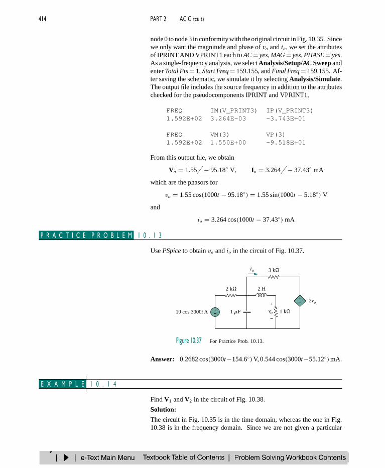
P R A C T I C E P R O B L E M 1 0 . 1 3
Use PSpice to obtain vo and io in the circuit of Fig. 10.37.
1 mF
2 H2 kΩ
3 kΩ
1 kΩ
io
2vo
+−10 cos 3000t A vo
+
−
+−
Figure 10.37 For Practice Prob. 10.13.
Answer: 0.2682 cos(3000t−154.6)V, 0.544 cos(3000t−55.12)mA.
E X A M P L E 1 0 . 1 4
Find V1 and V2 in the circuit of Fig. 10.38.
Solution:
The circuit in Fig. 10.35 is in the time domain, whereas the one in Fig.10.38 is in the frequency domain. Since we are not given a particular

CHAPTER 10 Sinusoidal Steady-State Analysis 415
2 Ω 2 ΩV1 V2
–j1 Ω
–j2
j2 Ω
–j1 Ω1 Ω3 0° A 18 30° V+−
j2 Ω
0.2Vx
−
+
Vx
Figure 10.38 For Example 10.14.
frequency and PSpice requires one, we select any frequency consistentwith the given impedances. For example, if we select ω = 1 rad/s, thecorresponding frequency is f = ω/2π = 0.159155 Hz. We obtain thevalues of the capacitance (C = 1/ωXC) and inductances (L = XL/ω).Making these changes results in the schematic in Fig. 10.39. To easewiring, we have exchanged the positions of the voltage-controlled cur-rent source G1 and the 2 + j2 impedance. Notice that the current ofG1 flows from node 1 to node 3, while the controlling voltage is acrossthe capacitor c2, as required in Fig. 10.38. The attributes of pseudocom-ponents VPRINT1 are set as shown. As a single-frequency analysis, weselect Analysis/Setup/AC Sweep and enter Total Pts = 1, Start Freq =0.159155, and Final Freq = 0.159155. After saving the schematic, weselect Analysis/Simulate to simulate the circuit. When this is done, theoutput file includes
FREQ VM(1) VP(1)1.592E-01 2.708E+00 -5.673E+01
FREQ VM(3) VP(3)1.592E-01 4.468E+00 -1.026E+02
AC=3
AC
R1I1
R2 L1
L2 R3
C1
C3G1 V1C21
2
3 45
0.5
2
2H
2H 2
1
11
AC=okMAG=okPHASE=ok
AC=okMAG=okPHASE=yes
ACMAG=18ACPHASE=30
0
GAIN=0.2
+ −+−−
−
Figure 10.39 Schematic for the circuit in Fig. 10.38.
416 PART 2 AC Circuits
from which we obtain
V1 = 2.708 − 56.73 V, V2 = 4.468 − 102.6 V
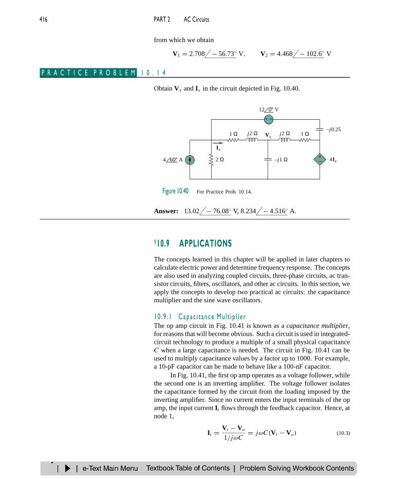
P R A C T I C E P R O B L E M 1 0 . 1 4
Obtain Vx and Ix in the circuit depicted in Fig. 10.40.
1 Ω 1 ΩVx
Ix
4Ix–j1 Ω
j2 Ω
2 Ω4 60° A
12 0° V
j2 Ω–j0.25
+ −
+−
Figure 10.40 For Practice Prob. 10.14.
Answer: 13.02 − 76.08 V, 8.234 − 4.516 A.
†10.9 APPLICATIONSThe concepts learned in this chapter will be applied in later chapters tocalculate electric power and determine frequency response. The conceptsare also used in analyzing coupled circuits, three-phase circuits, ac tran-sistor circuits, filters, oscillators, and other ac circuits. In this section, weapply the concepts to develop two practical ac circuits: the capacitancemultiplier and the sine wave oscillators.
10 . 9 . 1 Capac i t a n ce Mu l t i p l i e rThe op amp circuit in Fig. 10.41 is known as a capacitance multiplier,for reasons that will become obvious. Such a circuit is used in integrated-circuit technology to produce a multiple of a small physical capacitanceC when a large capacitance is needed. The circuit in Fig. 10.41 can beused to multiply capacitance values by a factor up to 1000. For example,a 10-pF capacitor can be made to behave like a 100-nF capacitor.
In Fig. 10.41, the first op amp operates as a voltage follower, whilethe second one is an inverting amplifier. The voltage follower isolatesthe capacitance formed by the circuit from the loading imposed by theinverting amplifier. Since no current enters the input terminals of the opamp, the input current Ii flows through the feedback capacitor. Hence, atnode 1,
Ii = Vi − Vo
1/jωC= jωC(Vi − Vo) (10.3)
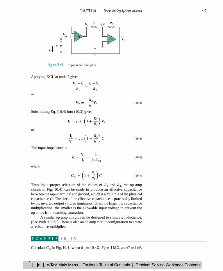
CHAPTER 10 Sinusoidal Steady-State Analysis 417
+
−
R1
A1
R2
+
−Vo
Ii
Zi
Vi
A2
C
0 V
2
1
+
−Vi
Figure 10.41 Capacitance multiplier.
Applying KCL at node 2 gives
Vi − 0
R1= 0 − Vo
R2
or
Vo = −R2
R1Vi (10.4)
Substituting Eq. (10.4) into (10.3) gives
Ii = jωC
(1 + R2
R1
)Vi
or
IiVi
= jω
(1 + R2
R1
)C (10.5)
The input impedance is
Zi = Vi
Ii= 1
jωCeq(10.6)
where
Ceq =(
1 + R2
R1
)C (10.7)
Thus, by a proper selection of the values of R1 and R2, the op ampcircuit in Fig. 10.41 can be made to produce an effective capacitancebetween the input terminal and ground, which is a multiple of the physicalcapacitance C. The size of the effective capacitance is practically limitedby the inverted output voltage limitation. Thus, the larger the capacitancemultiplication, the smaller is the allowable input voltage to prevent theop amps from reaching saturation.
A similar op amp circuit can be designed to simulate inductance.(See Prob. 10.69.) There is also an op amp circuit configuration to createa resistance multiplier.
E X A M P L E 1 0 . 1 5
CalculateCeq in Fig. 10.41 whenR1 = 10 k,R2 = 1 M, andC = 1 nF.
418 PART 2 AC Circuits
Solution:
From Eq. (10.7)
Ceq =(
1 + R2
R1
)C =
(1 + 1 × 10⁶
10 × 103
)1 nF = 101 nF
P R A C T I C E P R O B L E M 1 0 . 1 5
Determine the equivalent capacitance of the op amp circuit in Fig. 10.41if R1 = 10 k, R2 = 10 M, and C = 10 nF.
Answer: 10 µF.
10 . 9 . 2 Osc i l l a t o r sWe know that dc is produced by batteries. But how do we produce ac?One way is using oscillators, which are circuits that convert dc to ac.
An oscillator is a circuit that produces an ac waveform as outputwhen powered by a dc input.
The only external source an oscillator needs is the dc power supply.Ironically, the dc power supply is usually obtained by converting the acsupplied by the electric utility company to dc. Having gone through thetrouble of conversion, one may wonder why we need to use the oscillatorto convert the dc to ac again. The problem is that the ac supplied by theutility company operates at a preset frequency of 60 Hz in the UnitedStates (50 Hz in some other nations), whereas many applications suchas electronic circuits, communication systems, and microwave devicesrequire internally generated frequencies that range from 0 to 10 GHz orhigher. Oscillators are used for generating these frequencies.
This corresponds to ω = 2π f = 377 rad/s.
In order for sine wave oscillators to sustain oscillations, they mustmeet the Barkhausen criteria:
1. The overall gain of the oscillator must be unity or greater.Therefore, losses must be compensated for by an amplifyingdevice.
2. The overall phase shift (from input to output and back to theinput) must be zero.
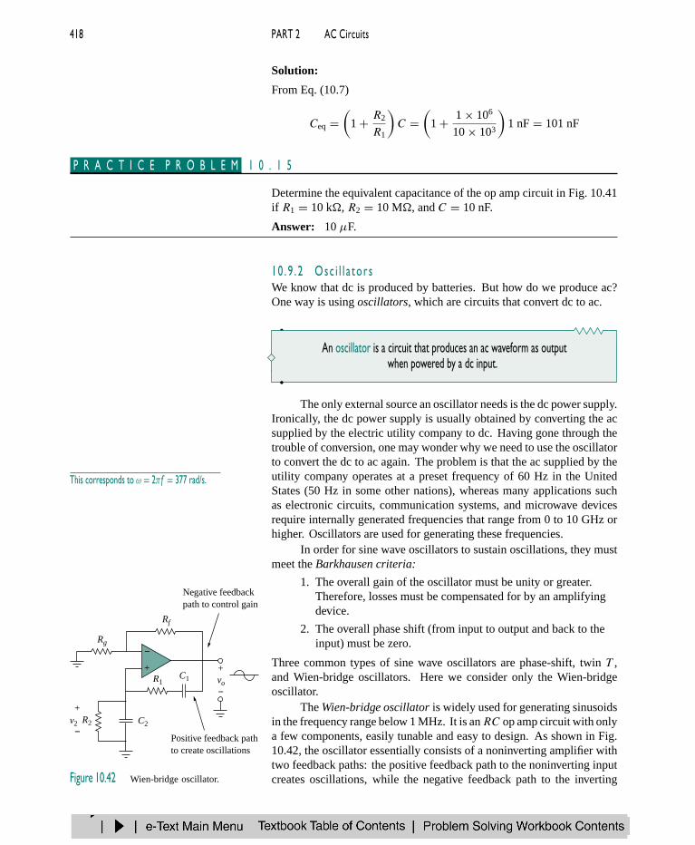
Three common types of sine wave oscillators are phase-shift, twin T ,and Wien-bridge oscillators. Here we consider only the Wien-bridgeoscillator.
+
−
Rf
Rg
R1
R2
C1
C2
+
−v2
+
−vo
Positive feedback pathto create oscillations
Negative feedbackpath to control gain
Figure 10.42 Wien-bridge oscillator.
The Wien-bridge oscillator is widely used for generating sinusoidsin the frequency range below 1 MHz. It is anRC op amp circuit with onlya few components, easily tunable and easy to design. As shown in Fig.10.42, the oscillator essentially consists of a noninverting amplifier withtwo feedback paths: the positive feedback path to the noninverting inputcreates oscillations, while the negative feedback path to the inverting

CHAPTER 10 Sinusoidal Steady-State Analysis 419
input controls the gain. If we define the impedances of the RC series andparallel combinations as Zs and Zp, then
Zs = R1 + 1
jωC1= R1 − j
ωC1(10.8)
Zp = R2 ‖ 1
jωC2= R2
1 + jωR2C2(10.9)
The feedback ratio is
V2
Vo
= Zp
Zs + Zp
(10.10)
Substituting Eqs. (10.8) and (10.9) into Eq. (10.10) gives
V2
Vo
= R2
R2 +(R1 − j
ωC1
)(1 + jωR2C2)
= ωR2C1
ω(R2C1 + R1C1 + R2C2) + j (ω2R1C1R2C2 − 1)
(10.11)
To satisfy the second Barkhausen criterion, V2 must be in phase with Vo,which implies that the ratio in Eq. (10.11) must be purely real. Hence,the imaginary part must be zero. Setting the imaginary part equal to zerogives the oscillation frequency ωo as
ω2oR1C1R2C2 − 1 = 0
or
ωo = 1√R1R2C1C2
(10.12)
In most practical applications, R1 = R2 = R and C1 = C2 = C, so that
ωo = 1
RC= 2πfo (10.13)
or
fo = 1
2πRC(10.14)
Substituting Eq. (10.13) and R1 = R2 = R, C1 = C2 = C into Eq.(10.11) yields
V2
Vo
= 1
3(10.15)
Thus in order to satisfy the first Barkhausen criterion, the op amp mustcompensate by providing a gain of 3 or greater so that the overall gain isat least 1 or unity. We recall that for a noninverting amplifier,
Vo
V2= 1 + Rf
Rg
= 3 (10.16)
or
Rf = 2Rg (10.17)
420 PART 2 AC Circuits
Due to the inherent delay caused by the op amp, Wien-bridge oscil-lators are limited to operating in the frequency range of 1 MHz or less.
E X A M P L E 1 0 . 1 6
Design a Wien-bridge circuit to oscillate at 100 kHz.
Solution:
Using Eq. (10.14), we obtain the time constant of the circuit as
RC = 1
2πfo= 1
2π × 100 × 103= 1.59 × 10⁻⁶ (10.16.1)
If we select R = 10 k, then we can select C = 159 pF to satisfy Eq.(10.16.1). Since the gain must be 3, Rf /Rg = 2. We could select Rf =20 k while Rg = 10 k.
P R A C T I C E P R O B L E M 1 0 . 1 6
In the Wien-bridge oscillator circuit in Fig. 10.42, let R1 = R2 = 2.5 k,C1 = C2 = 1 nF. Determine the frequency fo of the oscillator.
Answer: 63.66 kHz.
10.10 SUMMARY1. We apply nodal and mesh analysis to ac circuits by applying KCL
and KVL to the phasor form of the circuits.
2. In solving for the steady-state response of a circuit that has indepen-dent sources with different frequencies, each independent sourcemust be considered separately. The most natural approach to analyz-ing such circuits is to apply the superposition theorem. A separatephasor circuit for each frequency must be solved independently, andthe corresponding response should be obtained in the time domain.The overall response is the sum of the time-domain responses of allthe individual phasor circuits.
3. The concept of source transformation is also applicable in the fre-quency domain.
4. The Thevenin equivalent of an ac circuit consists of a voltage sourceVTh in series with the Thevenin impedance ZTh.
5. The Norton equivalent of an ac circuit consists of a current source INin parallel with the Norton impedance ZN (= ZTh).
6. PSpice is a simple and powerful tool for solving ac circuit problems.It relieves us of the tedious task of working with the complex num-bers involved in steady-state analysis.
7. The capacitance multiplier and the ac oscillator provide two typicalapplications for the concepts presented in this chapter. A capacitancemultiplier is an op amp circuit used in producing a multiple of aphysical capacitance. An oscillator is a device that uses a dc input togenerate an ac output.
CHAPTER 10 Sinusoidal Steady-State Analysis 421
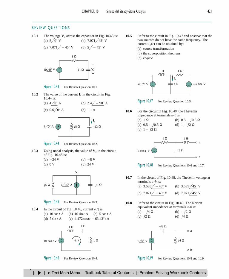
R E V I EW QU E S T I ON S
10.1 The voltage Vo across the capacitor in Fig. 10.43 is:(a) 5 0 V (b) 7.071 45 V
(c) 7.071 − 45 V (d) 5 − 45 V
1 Ω
+− Vo
+
−–j1 Ω10 0° V
Figure 10.43 For Review Question 10.1.
10.2 The value of the current Io in the circuit in Fig.10.44 is:(a) 4 0 A (b) 2.4 − 90 A
(c) 0.6 0 A (d) −1 A
j8 Ω –j2 Ω3 0° A
Io
Figure 10.44 For Review Question 10.2.
10.3 Using nodal analysis, the value of Vo in the circuitof Fig. 10.45 is:(a) −24 V (b) −8 V(c) 8 V (d) 24 V
–j3 Ωj6 Ω 4 90° A
Vo
Figure 10.45 For Review Question 10.3.
10.4 In the circuit of Fig. 10.46, current i(t) is:(a) 10 cos t A (b) 10 sin t A (c) 5 cos t A(d) 5 sin t A (e) 4.472 cos(t − 63.43) A
1 H 1 F
+− 1 Ω10 cos t V i(t)
Figure 10.46 For Review Question 10.4.
10.5 Refer to the circuit in Fig. 10.47 and observe that thetwo sources do not have the same frequency. Thecurrent ix(t) can be obtained by:(a) source transformation(b) the superposition theorem(c) PSpice
1 F+−
+−sin 2t V sin 10t V
1 H 1 Ω
ix
Figure 10.47 For Review Question 10.5.
10.6 For the circuit in Fig. 10.48, the Theveninimpedance at terminals a-b is:(a) 1 (b) 0.5 − j0.5
(c) 0.5 + j0.5 (d) 1 + j2
(e) 1 − j2
1 Ω 1 H
+− 1 F
a
b
5 cos t V
Figure 10.48 For Review Questions 10.6 and 10.7.
10.7 In the circuit of Fig. 10.48, the Thevenin voltage atterminals a-b is:(a) 3.535 − 45 V (b) 3.535 45 V
(c) 7.071 − 45 V (d) 7.071 45 V
10.8 Refer to the circuit in Fig. 10.49. The Nortonequivalent impedance at terminals a-b is:(a) −j4 (b) −j2
(c) j2 (d) j4
–j2 Ω
j4 Ω+−
a
b
6 0° V
Figure 10.49 For Review Questions 10.8 and 10.9.
422 PART 2 AC Circuits
10.9 The Norton current at terminals a-b in the circuit ofFig. 10.49 is:(a) 1 0 A (b) 1.5 − 90 A
(c) 1.5 90 A (d) 3 90 A
10.10 PSpice can handle a circuit with two independentsources of different frequencies.(a) True (b) False
Answers: 10.1c, 10.2a, 10.3d, 10.4a, 10.5b, 10.6c, 10.7a, 10.8a,10.9d, 10.10b.
P RO B L E M S
Section 10.2 Nodal Analysis
10.1 Find vo in the circuit in Fig. 10.50.
1 F+−
+−
1 H3 Ω
vo10 cos(t – 45°) V 5 sin(t + 30°) V+
−
Figure 10.50 For Prob. 10.1.
10.2 For the circuit depicted in Fig. 10.51 below,determine io.
10.3 Determine vo in the circuit of Fig. 10.52.
+−
2 H4 Ω
vo16 sin 4t V 2 cos 4t A+
−1 Ω 6 Ω
F112
Figure 10.52 For Prob. 10.3.
10.4 Compute vo(t) in the circuit of Fig. 10.53.
+−
1 H 0.25 F
1 Ω0.5ix vo
+
−16 sin (4t – 10°) V
ix
Figure 10.53 For Prob. 10.4.
10.5 Use nodal analysis to find vo in the circuit of Fig.10.54.
+−
10 mH50 mF20 Ω
20 Ω 30 Ω10 cos 103t V
io
4io vo
+
−
Figure 10.54 For Prob. 10.5.
10.6 Using nodal analysis, find io(t) in the circuit in Fig.10.55.
0.02 F+− 1 H
10 Ω
20 sin (10t – 4) V 4 cos (10t – 3) A
io
Figure 10.51 For Prob. 10.2.

CHAPTER 10 Sinusoidal Steady-State Analysis 423
0.5 F+−
1 H
2 H
2 Ω
0.25 F
8 sin (2t + 30°) V cos 2t A
io
Figure 10.55 For Prob. 10.6.
10.7 By nodal analysis, find io in the circuit in Fig. 10.56.
10 Ω
20 Ω 50 mF 10 mH20 sin1000t A
2io
io
Figure 10.56 For Prob. 10.7.
10.8 Calculate the voltage at nodes 1 and 2 in the circuitof Fig. 10.57 using nodal analysis.
10 Ω
1 2
–j2 Ω –j5 Ωj2 Ω
j4 Ω
20 30° A
Figure 10.57 For Prob. 10.8.
10.9 Solve for the current I in the circuit of Fig. 10.58using nodal analysis.
2 Ω
4 Ω–j2 Ω
j1 Ω
2I
5 0° A
20 –90° V +−
I
Figure 10.58 For Prob. 10.9.
10.10 Using nodal analysis, find V1 and V2 in the circuitof Fig. 10.59.
20 Ω
10 Ω
j2 A 1 + j A
–j5 Ω
j10 Ω
V1 V2
Figure 10.59 For Prob. 10.10.
10.11 By nodal analysis, obtain current Io in the circuit inFig. 10.60.
3 Ω
2 Ω1 Ωj4 Ω
–j2 Ω
+−100 20° V
Io
Figure 10.60 For Prob. 10.11.
10.12 Use nodal analysis to obtain Vo in the circuit of Fig.10.61 below.
8 Ω
2 Ω –j1 Ω –j2 Ω
j6 Ω 4 Ω j5 Ω
2Vx Vo4 45° A
+
−Vx
+
−
Figure 10.61 For Prob. 10.12.
424 PART 2 AC Circuits
10.13 Obtain Vo in Fig. 10.62 using nodal analysis.
4 Ω
2 Ω –j4 Ω
j2 Ω
Vo 0.2Vo
+
−
+ −
12 0° V
Figure 10.62 For Prob. 10.13.
10.14 Refer to Fig. 10.63. If vs(t) = Vm sinωt andvo(t) = A sin(ωt + φ), derive the expressions for Aand φ.
+− vo(t)vs(t)
+
−L
R
C
Figure 10.63 For Prob. 10.14.
10.15 For each of the circuits in Fig. 10.64, find Vo/Vi forω = 0, ω → ∞, and ω2 = 1/LC.
Vo
+
−
Vo
+
−
Vi
+
−
Vi
+
−
C
R R CL
L
(b)(a)
Figure 10.64 For Prob. 10.15.
10.16 For the circuit in Fig. 10.65, determine Vo/Vs .
+−Vs Vo
+
−L
R1
R2
C
Figure 10.65 For Prob. 10.16.
Section 10.3 Mesh Analysis
10.17 Obtain the mesh currents I1 and I2 in the circuit ofFig. 10.66.
+−Vs L
R
C2
C1
I2I1
Figure 10.66 For Prob. 10.17.
10.18 Solve for io in Fig. 10.67 using mesh analysis.
+−
+−
2 H
0.25 F
4 Ω
10 cos 2t V 6 sin 2t V
io
Figure 10.67 For Prob. 10.18.
10.19 Rework Prob. 10.5 using mesh analysis.
10.20 Using mesh analysis, find I1 and I2 in the circuit ofFig. 10.68.
+−
+−I2I1
j10 Ω
–j20 Ω
40 Ω
50 0° V40 30° V
Figure 10.68 For Prob. 10.20.
10.21 By using mesh analysis, find I1 and I2 in the circuitdepicted in Fig. 10.69.
I2I1
j4 Ω
j2 Ω
j1 Ω
–j6 Ω
3 Ω
2 Ω
30 20° V
3 Ω
+ −
Figure 10.69 For Prob. 10.21.
CHAPTER 10 Sinusoidal Steady-State Analysis 425
10.22 Repeat Prob. 10.11 using mesh analysis.
10.23 Use mesh analysis to determine current Io in thecircuit of Fig. 10.70 below.
10.24 Determine Vo and Io in the circuit of Fig. 10.71using mesh analysis.
j4 Ω
Io
3Vo –j2 Ω4 –30° A 2 Ω +−Vo
+
−
Figure 10.71 For Prob. 10.24.
10.25 Compute I in Prob. 10.9 using mesh analysis.
10.26 Use mesh analysis to find Io in Fig. 10.28 (forExample 10.10).
10.27 Calculate Io in Fig. 10.30 (for Practice Prob. 10.10)using mesh analysis.
10.28 Compute Vo in the circuit of Fig. 10.72 using meshanalysis.
–j3 Ω
2 Ω
j4 Ω
+−2 Ω
2 Ω12 0° V
2 0° A
4 90° A Vo
+
−
Figure 10.72 For Prob. 10.28.
10.29 Using mesh analysis, obtain Io in the circuit shownin Fig. 10.73.
–j4 Ωj2 Ω2 Ω
1 Ω 1 Ω
Io
+− 10 90° V
4 0° A
2 0° A
Figure 10.73 For Prob. 10.29.
Section 10.4 Superposition Theorem
10.30 Find io in the circuit shown in Fig. 10.74 usingsuperposition.
4 Ω
+−
+−
2 Ω
8 V1 H10 cos 4t V
io
Figure 10.74 For Prob. 10.30.
10.31 Using the superposition principle, find ix in thecircuit of Fig. 10.75.
+−
3 Ω
4 H 10 cos(2t – 60°) V5 cos(2t + 10°) A
ixF1
8
Figure 10.75 For Prob. 10.31.
10.32 Rework Prob. 10.2 using the superposition theorem.
10.33 Solve for vo(t) in the circuit of Fig. 10.76 using thesuperposition principle.
–j40 Ω –j40 Ω
j60 Ω80 Ω 20 ΩIo
+−
+−100 120° V 60 –30° V
Figure 10.70 For Prob. 10.23.
426 PART 2 AC Circuits
+−
+−
6 Ω 2 H
10 V12 cos 3t V 4 sin 2t A+
−voF1
12
Figure 10.76 For Prob. 10.33.
10.34 Determine io in the circuit of Fig. 10.77.
+−
1 Ω 2 H24 V
2 cos 3t2 Ω 4 Ω
+−io
10 sin(3t – 30°) V
F16
Figure 10.77 For Prob. 10.34.
10.35 Find io in the circuit in Fig. 10.78 usingsuperposition.
80 Ω
60 Ω
40 mH
20 mF
24 V
100 Ω
+−
+−50 cos 2000t V
2 sin 4000t A
io
Figure 10.78 For Prob. 10.35.
Section 10.5 Source Transformation
10.36 Using source transformation, find i in the circuit ofFig. 10.79.
3 Ω
5 Ω5 mH
1 mF
8 sin(200t + 30°) A
i
Figure 10.79 For Prob. 10.36.
10.37 Use source transformation to find vo in the circuit inFig. 10.80.
20 Ω
80 Ω
0.4 mH
0.2 mF+−5 cos 105t V vo
+
−
Figure 10.80 For Prob. 10.37.
10.38 Solve Prob. 10.20 using source transformation.
10.39 Use the method of source transformation to find Ixin the circuit of Fig. 10.81.
+−
2 Ω j4 Ω –j2 Ω
–j3 Ω
6 Ω 4 Ω
Ix
60 0° V 5 90° A
Figure 10.81 For Prob. 10.39.
10.40 Use the concept of source transformation to find Vo
in the circuit of Fig. 10.82.
+−
4 Ω j4 Ω–j3 Ω
–j2 Ωj2 Ω 2 Ω20 0° V Vo
+
−
Figure 10.82 For Prob. 10.40.
Section 10.6 Thevenin and Norton EquivalentCircuits
10.41 Find the Thevenin and Norton equivalent circuits atterminals a-b for each of the circuits in Fig. 10.83.
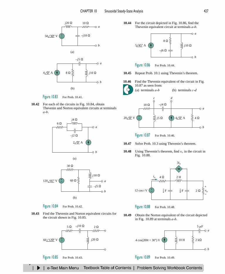
CHAPTER 10 Sinusoidal Steady-State Analysis 427
–j10 Ω
j20 Ω 10 Ωa
b
50 30° V +−
a
b
4 0° A
–j5 Ω
j10 Ω8 Ω
(b)
(a)
Figure 10.83 For Prob. 10.41.
10.42 For each of the circuits in Fig. 10.84, obtainThevenin and Norton equivalent circuits at terminalsa-b.
–j5 Ω
j4 Ω6 Ω
30 Ω
a
b
2 0° A
a
b
120 45° V
–j2 Ω
j10 Ω
60 Ω
(b)
(a)
+−
Figure 10.84 For Prob. 10.42.
10.43 Find the Thevenin and Norton equivalent circuits forthe circuit shown in Fig. 10.85.
j20 Ω
5 Ω 2 Ω
60 120° V +−
–j10 Ω
Figure 10.85 For Prob. 10.43.
10.44 For the circuit depicted in Fig. 10.86, find theThevenin equivalent circuit at terminals a-b.
a
b
5 45° A j10 Ω8 Ω
–j6 Ω
Figure 10.86 For Prob. 10.44.
10.45 Repeat Prob. 10.1 using Thevenin’s theorem.
10.46 Find the Thevenin equivalent of the circuit in Fig.10.87 as seen from:(a) terminals a-b (b) terminals c-d
10 Ωa
b
4 0° A20 0° V
–j4 Ω
j5 Ω 4 Ω+−
c d
Figure 10.87 For Prob. 10.46.
10.47 Solve Prob. 10.3 using Thevenin’s theorem.
10.48 Using Thevenin’s theorem, find vo in the circuit inFig. 10.88.
2 H4 Ω
2 Ω vo
io
3io
+−12 cos t V
+
−F1
4 F18
Figure 10.88 For Prob. 10.48.
10.49 Obtain the Norton equivalent of the circuit depictedin Fig. 10.89 at terminals a-b.
a
b
5 mF
10 H 2 kΩ4 cos(200t + 30°) V
Figure 10.89 For Prob. 10.49.

428 PART 2 AC Circuits
10.50 For the circuit shown in Fig. 10.90, find the Nortonequivalent circuit at terminals a-b.
60 Ω 40 Ω
–j30 Ωj80 Ω
a b3 60° A
Figure 10.90 For Prob. 10.50.
10.51 Compute io in Fig. 10.91 using Norton’s theorem.
2 Ω
4 H
5 cos 2t V
+ −io
F14 F1
2
Figure 10.91 For Prob. 10.51.
10.52 At terminals a-b, obtain Thevenin and Nortonequivalent circuits for the network depicted in Fig.10.92. Take ω = 10 rad/s.
a
b
10 mF
10 Ω2 sin vt V
12 cos vt+−
vo 2vo
+
−H1
2
Figure 10.92 For Prob. 10.52.
Section 10.7 Op Amp AC Circuits
10.53 For the differentiator shown in Fig. 10.93, obtainVo/Vs . Find vo(t) when vs(t) = Vm sinωt andω = 1/RC.
+−vs vo
R
C
+
−
+−
Figure 10.93 For Prob. 10.53.
10.54 The circuit in Fig. 10.94 is an integrator with afeedback resistor. Calculate vo(t) ifvs = 2 cos 4 × 10⁴t V.
+−vs vo
+
−
10 nF
100 kΩ
50 kΩ
+−
Figure 10.94 For Prob. 10.54.
10.55 Compute io(t) in the op amp circuit in Fig. 10.95 ifvs = 4 cos 104t V.
+−vs
50 kΩ
1 nF100 kΩ
io
+−
Figure 10.95 For Prob. 10.55.
10.56 If the input impedance is defined as Zin = Vs/Is ,find the input impedance of the op amp circuit inFig. 10.96 when R1 = 10 k, R2 = 20 k,C1 = 10 nF, C2 = 20 nF, and ω = 5000 rad/s.
Vs C2
C1
R1 R2Is
Zin
Vo
+−
+−
Figure 10.96 For Prob. 10.56.
10.57 Evaluate the voltage gain Av = Vo/Vs in the opamp circuit of Fig. 10.97. Find Av at ω = 0,ω → ∞, ω = 1/R1C1, and ω = 1/R2C2.
+−Vs Vo
+
−
C1R1
C2R2
+−
Figure 10.97 For Prob. 10.57.

CHAPTER 10 Sinusoidal Steady-State Analysis 429
10.58 In the op amp circuit of Fig. 10.98, find theclosed-loop gain and phase shift if C1 = C2 = 1 nF,R1 = R2 = 100 k, R3 = 20 k, R4 = 40 k, andω = 2000 rad/s.
vs vo
C1
R1
R2+−
C2
R4
R3
+
−
+−
Figure 10.98 For Prob. 10.58.
10.59 Compute the closed-loop gain Vo/Vs for the op ampcircuit of Fig. 10.99.
+
−
+−vs
vo
+
−
C1
R1
R3 C2 R2
Figure 10.99 For Prob. 10.59.
10.60 Determine vo(t) in the op amp circuit in Fig. 10.100below.
10.61 For the op amp circuit in Fig. 10.101, obtain vo(t).
vo+−
10 kΩ
20 kΩ
40 kΩ0.1 mF
0.2 mF
+−
+−
+
−
5 cos 103t V
Figure 10.101 For Prob. 10.61.
10.62 Obtain vo(t) for the op amp circuit in Fig. 10.102 ifvs = 4 cos(1000t − 60) V.
vovs +
−
10 kΩ
50 kΩ
20 kΩ 0.2 mF
0.1 mF
+−
+−
+
−
Figure 10.102 For Prob. 10.62.
Section 10.8 AC Analysis Using PSpice
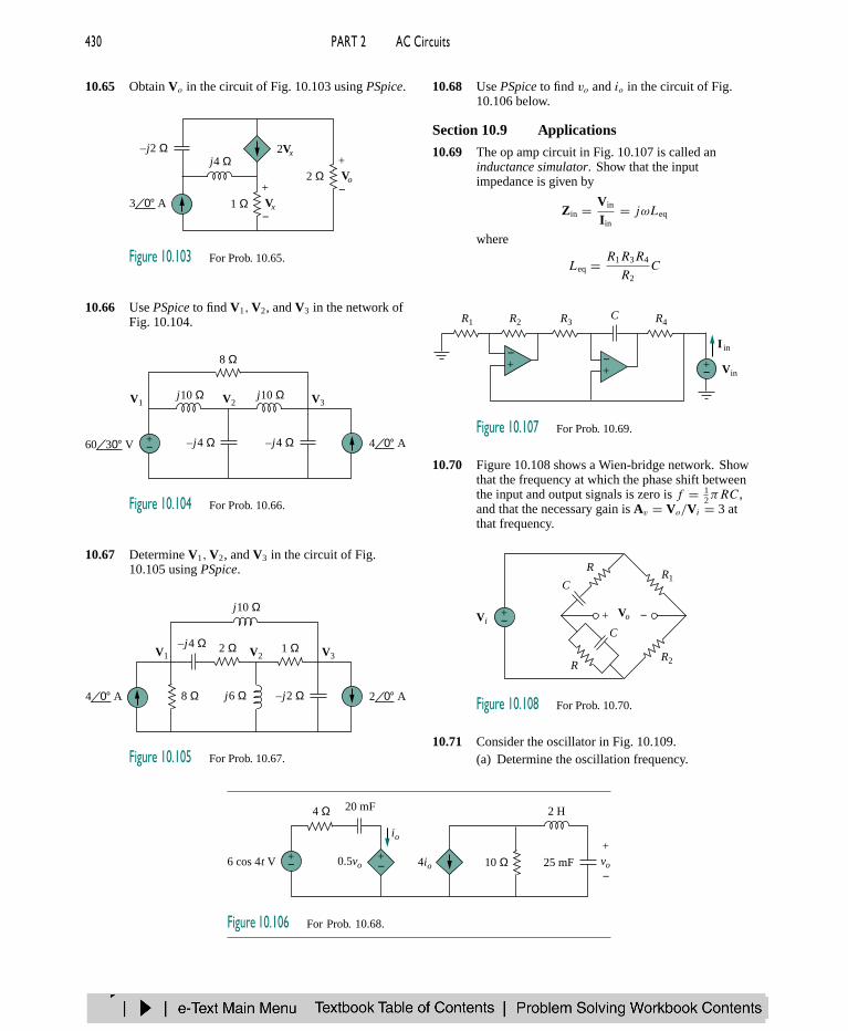
10.63 Use PSpice to solve Example 10.10.
10.64 Solve Prob. 10.13 using PSpice.
vo
+−
10 kΩ
20 kΩ
20 kΩ
40 kΩ10 kΩ0.25 mF
0.5 mF
+−
2 sin 400t V
Figure 10.100 For Prob. 10.60.
430 PART 2 AC Circuits
10.65 Obtain Vo in the circuit of Fig. 10.103 using PSpice.
1 Ω
j4 Ω–j2 Ω
2 Ω+
−Vx
2Vx+
−Vo
3 0° A
Figure 10.103 For Prob. 10.65.
10.66 Use PSpice to find V1,V2, and V3 in the network ofFig. 10.104.
+−
8 Ω
j10 Ω j10 Ω
–j4 Ω –j4 Ω
V1 V3V2
60 30° V 4 0° A
Figure 10.104 For Prob. 10.66.
10.67 Determine V1,V2, and V3 in the circuit of Fig.10.105 using PSpice.
8 Ω
j10 Ω
1 Ω2 Ω
j6 Ω –j2 Ω
–j4 ΩV1 V3V2
4 0° A 2 0° A
Figure 10.105 For Prob. 10.67.
10.68 Use PSpice to find vo and io in the circuit of Fig.10.106 below.
Section 10.9 Applications
10.69 The op amp circuit in Fig. 10.107 is called aninductance simulator. Show that the inputimpedance is given by
Zin = Vin
Iin= jωLeq
where
Leq = R1R3R4
R2C
Vin
I in
+−
+−
R1 R2 R3C R4
+−
Figure 10.107 For Prob. 10.69.
10.70 Figure 10.108 shows a Wien-bridge network. Showthat the frequency at which the phase shift betweenthe input and output signals is zero is f = 1
2πRC,and that the necessary gain is Av = Vo/Vi = 3 atthat frequency.
Vi+−
RR1
R2R
C
C
+ −Vo
Figure 10.108 For Prob. 10.70.
10.71 Consider the oscillator in Fig. 10.109.(a) Determine the oscillation frequency.
20 mF
25 mF
2 H4 Ω
10 Ω vo0.5vo
io
4io+−6 cos 4t V
+
−
+−
Figure 10.106 For Prob. 10.68.
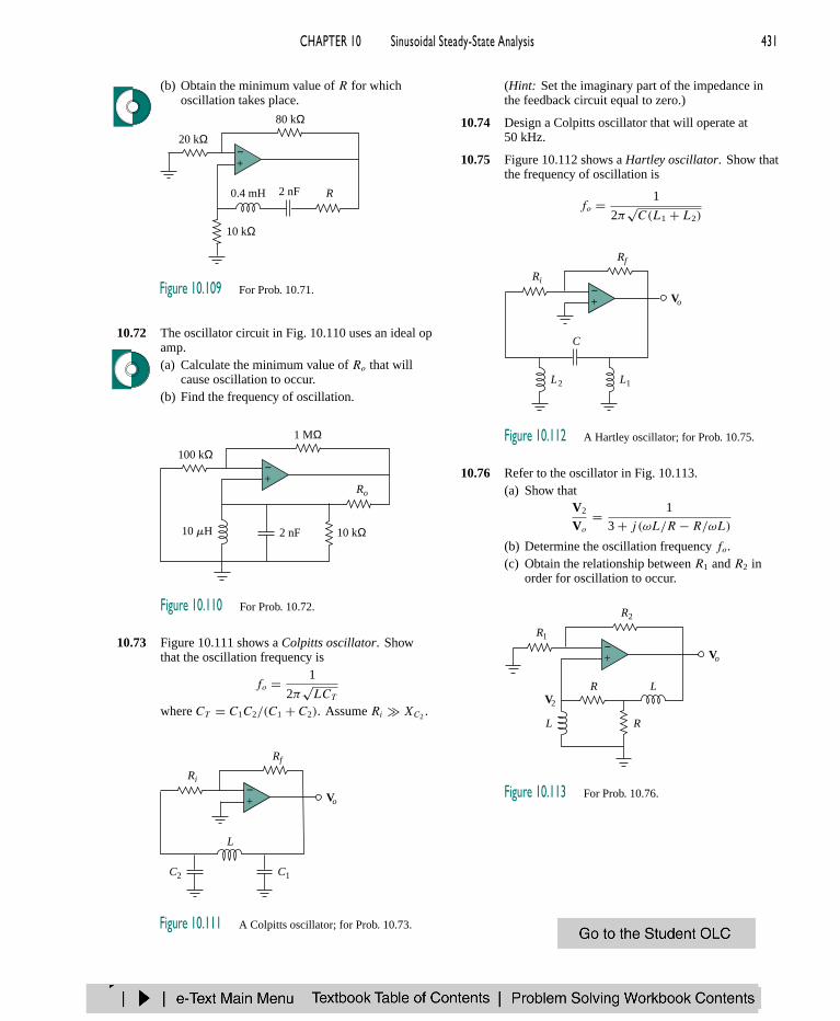
CHAPTER 10 Sinusoidal Steady-State Analysis 431
(b) Obtain the minimum value of R for whichoscillation takes place.
+−
R
10 kΩ
20 kΩ
80 kΩ
0.4 mH 2 nF
Figure 10.109 For Prob. 10.71.
10.72 The oscillator circuit in Fig. 10.110 uses an ideal opamp.(a) Calculate the minimum value of Ro that will
cause oscillation to occur.(b) Find the frequency of oscillation.
+−
10 kΩ
100 kΩ
1 MΩ
10 mH 2 nF
Ro
Figure 10.110 For Prob. 10.72.
10.73 Figure 10.111 shows a Colpitts oscillator. Showthat the oscillation frequency is
fo = 1
2π√LCT
where CT = C1C2/(C1 + C2). Assume Ri XC2 .
+−
Rf
Ri
C2 C1
L
Vo
Figure 10.111 A Colpitts oscillator; for Prob. 10.73.
(Hint: Set the imaginary part of the impedance inthe feedback circuit equal to zero.)
10.74 Design a Colpitts oscillator that will operate at50 kHz.
10.75 Figure 10.112 shows a Hartley oscillator. Show thatthe frequency of oscillation is
fo = 1
2π√C(L1 + L2)
+−
Rf
Ri
L2 L1
C
Vo
Figure 10.112 A Hartley oscillator; for Prob. 10.75.
10.76 Refer to the oscillator in Fig. 10.113.(a) Show that
V2
Vo
= 1
3 + j (ωL/R − R/ωL)
(b) Determine the oscillation frequency fo.(c) Obtain the relationship between R1 and R2 in
order for oscillation to occur.
+−
R L
RL
R1
R2
Vo
V2
Figure 10.113 For Prob. 10.76.


![EE152F1 4Midterm Solutions - Stanford University · 3$ $ 15$ 4$ $ 15$ 5$ $ 15$ 6$ $ 20$ 7$ $ 20$ Total$ $ 120$!!! V0.5! ! ! Page!! 2! Problem!1:!!Periodic!Steady!StateAnalysis![20!Points]!!](https://img.dokumen.tips/doc/110x75/5f1a1955025bcd2f3f0fc651/ee152f1-4midterm-solutions-stanford-university-3-15-4-15-5-15-6-.jpg)