Embed Size (px)
Citation preview
10-1
Chapter 10 Physics of
Electrons
Contents
Chapter 10 Physics of Electrons ................................................................................... 10-1
Contents .......................................................................................................................... 10-1 10.1 Quantum Mechanics .......................................................................................... 10-2
10.1.1 Electromagnetic Wave ............................................................................... 10-2 10.1.2 Atomic Structure ........................................................................................ 10-4
10.1.3 Bohr’s model .............................................................................................. 10-6 10.1.4 Line Spectra ............................................................................................... 10-8
10.1.5 De Broglie Wave........................................................................................ 10-9 10.1.6 Heisenberg Uncertainty Principle ............................................................ 10-10
10.1.7 Schrödinger Equation............................................................................... 10-11 10.1.8 A Particle in a 1-D Box ............................................................................ 10-12 10.1.9 Quantum Numbers ................................................................................... 10-16
10.1.10 Electron Configurations ........................................................................... 10-18 Example 10.1 Electronic Configuration of a Silicon Atom ...................................... 10-20
10.2 Band Theory and Doping ................................................................................. 10-21
10.2.1 Covalent Bonding .................................................................................... 10-21 10.2.2 Energy Band............................................................................................. 10-21
10.2.3 Pseudo-Potential Well .............................................................................. 10-23
10.2.4 Doping, Donors, and Acceptors ............................................................... 10-23 Problems ....................................................................................................................... 10-25

10-2
10.1 Quantum Mechanics
10.1.1 Electromagnetic Wave
Light is known to have a wave-particle dual nature. The phenomena of light propagation may best
be described by the electromagnetic wave theory, while the interaction of light with matter is best
described as a particle phenomenon.
Maxwell (1864) showed theoretically that electrical disturbance should propagate in free space
with a speed equal to that of light, which gives that light waves are indeed electromagnetic waves.
These waves are also known as radio and television transmission, X-Ray, and many other
examples. Electromagnetic waves are produced whenever electric charges are accelerated. Lights
consists of oscillating electric (E) and magnetic (H) fields that are perpendicular to each other and
to the direction of the light, as shown in Figure 10.1. The wavelength is indicated in the figure.
Figure 10.1 Lights consists of oscillating electric (E) and magnetic (H) fields that are
perpendicular to each other.
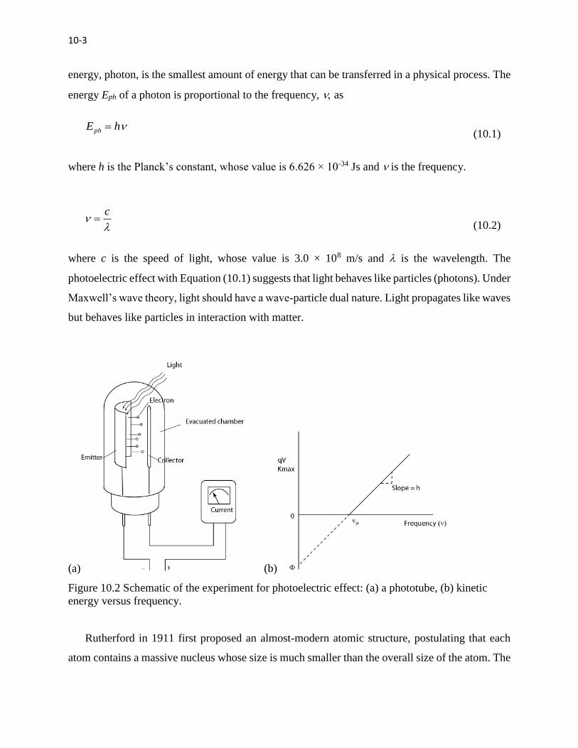
Hertz (1887) first observed that electrons were emitted when light strokes a metal surface. A
modern phototube is shown schematically in Figure 10.2. What was particularly puzzling about
this photoelectric effect was that no matter how intense the light shines on the metal surface, if the
frequency of the light is below a specific minimum value, no electron is emitted. The photoelectric
effect could not be explained by classical physics. According to classical theory, the energy
associated with electromagnetic radiation depends only on the intensity and not on the frequency.
The correct explanation of the photoelectric effect was given by Einstein in 1905, postulating
that a beam of light consisted of small quanta of energy that are now called photons, and that an
electron in the metal absorbs the incident photon’s energy required to escape from the metal, which
is an all-or-none process—the electron getting all the photon’s energy or none at all. The quantum
10-3
energy, photon, is the smallest amount of energy that can be transferred in a physical process. The
energy Eph of a photon is proportional to the frequency, as
hEph (10.1)
where h is the Planck’s constant, whose value is 6.626 × 10⁻³⁴ Js and is the frequency.
c
(10.2)
where c is the speed of light, whose value is 3.0 × 10⁸ m/s and is the wavelength. The
photoelectric effect with Equation (10.1) suggests that light behaves like particles (photons). Under
Maxwell’s wave theory, light should have a wave-particle dual nature. Light propagates like waves
but behaves like particles in interaction with matter.
(a) (b)
Figure 10.2 Schematic of the experiment for photoelectric effect: (a) a phototube, (b) kinetic
energy versus frequency.
Rutherford in 1911 first proposed an almost-modern atomic structure, postulating that each
atom contains a massive nucleus whose size is much smaller than the overall size of the atom. The

10-4
nucleus is surrounded by a swarm of electrons that revolve around the nucleus in orbits, more or
less as the planets in the solar system revolve around the Sun. The Rutherford’s planetary model
faced a dilemma, however. A charged electron in orbit should be unstable and spiral into the
nucleus and come to rest, because a charged particle in an orbit should be accelerated toward the
center and emit radiation, owing to the electromagnetic wave theory. Instead, observation showed
stable atoms without emitting radiation from electrons in orbits. There is an obvious defect in the
planetary model.
In 1913, Bohr proposed a new model, assuming that the angular momentum is quantized and
must be an integer multiple of h/2. He postulated that an electron in an atom can revolve in certain
stable orbits, each having a definite associated energy, without emitting radiation. Bohr’s model
was successful in accounting for many atomic observations, especially the emission and absorption
spectra for hydrogen. Despite these successes, it cannot predict the energy levels and spectra of
atoms with more than one electron. The postulate of quantized angular momentum had no
fundamental basis.
In 1924, de Broglie proposed that not only light but all matter, including electrons, has a wave-
particle dual nature. De Broglie’s work attributed wavelike properties to electrons in atoms, and
the Heisenberg uncertainty principle (1927) shows that detailed trajectories of electrons cannot be
defined. Consequently, it must be dealt with in terms of the probability of electrons having certain
positions and momenta. These ideas were combined in the fundamental equation of quantum
mechanics, the Schrödinger equation, discovered by the Erwin Schrödinger in 1925. Bohr’s theory
was replaced by modern quantum mechanics, in which the quantization of energy and angular
momentum is a natural consequence of the basic postulates and requires no extra assumptions.
10.1.2 Atomic Structure
Each atom consists of a very small nucleus which is composed of protons and neutrons. The
nucleus is encircled by moving electrons. Both electrons and protons are electrically charged, the
charge magnitude being 1.6 × 10⁻¹⁹ Coulomb (C), which is negative in sign for electrons and
positive for protons; neutrons are electrically neutral. An atom containing an equal number of
protons and electrons is electrically neutral: otherwise, it has a positive or negative charge and is
an ion. When an electron is bound to an atom, it has a potential energy that is inversely proportional

10-5
to its distance from the nucleus. This is measured by the amount of energy needed to unbind the
electron from the atom, and is usually given in units of electron volt (eV).
Masses for these subatomic particles are infinitesimally small; protons and neutrons have
approximately the same mass, 1.67 × 10⁻²⁷ kg, which is significantly larger than that for an electron,
9.11 × 10⁻³¹ kg.
The most obvious feature of an atomic nucleus is its size, about 200,000 times smaller than the
atom itself. The radius of a nucleus is about 1.2 × 10⁻¹⁵ m, where the electron orbits the nucleus
with a radius of 1 × 10⁻¹⁰ m, as shown in Figure 10.3. If the nucleus were the size of a basketball,
the diameter of the atom would be about 24 kilometers (15 miles). Table 10.1 and Table 10.2
summarize properties of an atom.
Figure 10.3 Schematic of an atomic structure.
Table 10.1 Summary of Information Related to an Atom
Description Mass Charge
Electron mass me = 9.10939 × 10⁻³¹ kg q = 1.6021 × 10⁻¹⁹ C = 1 eV/V
Proton mass 1.6726 x 10⁻²⁷ kg +1.6021 × 10⁻¹⁹ C
Neutron mass 1.6929 x 10⁻²⁷ kg neutral
Table 10.2 Physical Constants and Units
Description Symbol Value
Electron volt eV 1 eV = 1.6021 × 10⁻¹⁹ J
Planck’s constant h h = 6.62608 × 10⁻³⁴ Js=4.135 × 10⁻¹⁵ eV-s
Boltzmann’s constant kB kB = 1.38066 × 10⁻²³ J/K=8.617 × 10-5 eV/K
Permittivity of vacuum (free space) 0 0 = 8.854 × 10⁻¹² C2·J-1·m-1 = 8.854 × 10⁻¹⁴ CV-1cm-1
Dielectric constant of Si Ks Ks

10-6
kT kT 0.0259 eV (T = 300K)
10.1.3 Bohr’s model
In 1913, Niels Bohr developed a model for the atom that accounted for the striking regularities
seen in the spectrum of the hydrogen atom. Bohr supplemented the Rutherford’s planetary model
of atom with the assumption that an electron of mass me moves in a circular orbit of radius r about
a fixed nucleus. Bohr assumed that the angular momentum is quantized and must be an integer
multiple of h/2.
π2
hnvrme
(10.3)
where me is the mass of electron, v the velocity, r the radius, and n = 1,2,3, etc. According to
Coulomb’s law, the attraction force of two charges, Ze and e, separated by a distance r is
2
04
1
r
eZeF
(10.4)
From Newton’s law,
r
vmamF ee
2
(10.5)
Combining Equations (10.3) and (10.5) and solving for r and v, we obtain
emZe
hnr
2
22
0
(10.6)
nh
Zev
0
2
2
(10.7)
where Z is the atomic number, e is the electronic charge, and 0 is the permittivity of a vacuum.
Hence, the radius of the first Bohr’s orbit for n = 1 hydrogen is calculated using Table 10.1 and
Table 10.2 for the physical constants as

10-7
m100.53
kg109.109C101.60213.14
sJ106.6261mJC108.854 10
31219
234211212
r
(10.8)
This is in good agreement with atomic diameters as estimated by other methods, namely about 10-
10 m (see Figure 10.3). And the velocity of the electron of the first Bohr’s orbit for hydrogen is
calculated as
m/s102.19
sJ106.6261mJC108.8542
C101.6021 6
3411212
219
v
(10.9)
The velocity of the electron is barely discussed in the literature being much smaller than the speed
of light (3 × 10⁸ m/s). According to the Heisenberg uncertainty principle, this velocity is not known
precisely (as a cloud-probability). However, the Bohr’s velocity gives a good intuition of the
atomic structure.
Next, by examining the kinetic energy [1] and potential energy (P.E) components of the total
electron energy in the various orbits, we find the K.E using Equation (10.7) as
222
0
422
0
22
822
1
2
1.
hn
meZ
nh
ZemvmEK e
ee
(10.10)
Setting P.E = 0 at r = as a boundary condition, we have
r
e
rhn
meZ
r
Zedr
r
eZeFdrEP
222
0
42
0
2
2
0 4
1
44
1.
(10.11)
The total energy that is sometimes referred to as binding energy is therefore,
222
0
42
8..
hn
meZEPEKE e
n
,.....3,2,1n (10.12)

10-8
Figure 10.4 Energy level diagram for the hydrogen atom
10.1.4 Line Spectra
Bohr’s model thus predicts a discrete energy level diagram for a one-electron atom, which means
that the electron is allowed to stay only in one of the quantized energy levels described in Equation
(10.12), which is schematically shown in Figure 10.4. The ground state for the system of nucleus
plus electron has n = 1; excited states have higher values of n. When the binding energy turns to
zero at n = , the electron becomes a free electron from the atom. The electron that receives
energy from a perturbation such as sunlight, electric field, kinetic energy of other moving
electrons, or even thermal energy should jump up to a higher energy level, as shown in the figure.
Usually the exited electron is unstable and returns back to a lower level of energy, emitting a
photon with energy that is exactly the same as the energy difference of the higher and lower energy
levels. The energy difference is easily calculated using Equation (10.12) with Equation (10.1) as
2222
0
4211
8 fi
efi
nnh
meZchhEEE
(10.13)
Solving for the frequency or we have
2232
0
4211
8 fi
e
nnh
meZc
(10.14)

10-9
Equation (10.14) is in good agreement with the measured line spectra for a hydrogen atom, as
shown in Figure 10.5. For example, Red 656 nm indicates a spectrum with the wavelength of 656
nm (nanometer, 10-9 m), of which the indicated line may be understandable when considering the
visible spectrum of light (rainbow) ranging from 400 nm to 700 nm, where the color ranges from
violet to red. The measured spectrum of Red 656 nm in Figure 10.5 can be calculated from
Equation (10.14) by varying the quantum number from n = 3 to n = 2. In the same way, Blue 486
nm from n = 4 to n= 2 and Violet 434 nm from n = 5 to n = 2. Equation (10.14) was used to directly
identify the line spectra from unknown materials such as a spectrum from stars far away at one-
billion-year distance. For example, helium was discovered by studying the line spectra from the
Sun during the solar eclipse in 1868 even before the helium was found on the Earth in 1895.
Figure 10.5 Schematic diagrams of the line spectra for a hydrogen atom
10.1.5 De Broglie Wave
Although the Bohr model was immensely successful in explaining the hydrogen spectra, numerous
attempts to extend the semiclassical Bohr analysis to more complex atoms such as helium proved
to be futile. Moreover, the quantization of angular momentum in the Bohr model had no theoretical
basis.
In 1924, de Broglie postulated that if light has the dual properties of waves and particles,
electrons should have duality also. He suggested that an electron in an atom might be associated
with a circular standing wave, as shown in Figure 10.6. The condition for the circular standing
wave is
rn 2 (10.15)
Combing Equation (10.15) and the Bohr’s assumption of Equation (10.3), we obtain the
wavelength as
400 450 500 550 600 650 700
Wavelength (nm)
Violet 434 nm Blue 486 nm Red 656 nm

10-10
p
h
vm
h
e
(10.16)
It is very important to note that the wavelength is related to the linear momentum p of the electron
or a particle. De Broglie showed with the theory of relativity that exactly the same relationship
holds between the wavelength and momentum of a photon. De Broglie therefore proposed as a
generalization that any particle moving with linear momentum p has wavelike properties and a
wavelength associated with it. Within three years, two different experiments had been performed
to demonstrate that electrons do exhibit wave behavior. De Broglie was the first of only two
physicists to receive a Nobel Prize for his thesis work.
Figure 10.6 Electrons form standing wave about the nucleus
10.1.6 Heisenberg Uncertainty Principle
In 1927, Werner Heisenberg stated the uncertainty principle that the position and the velocity of a
particle on an atomic scale cannot be simultaneously determined with precision. Mathematically,
it says that the product of the uncertainties of these pairs has a lower limit equal to Planck’s
constant
Δ𝑥Δ𝑝 ≥ℏ
2 (10.17a)
where x is the uncertainty of the position and p is the uncertainty of the momentum or the
velocity and there is also an uncertainty principle in energy and time. From the second uncertainty
relation,
10-11
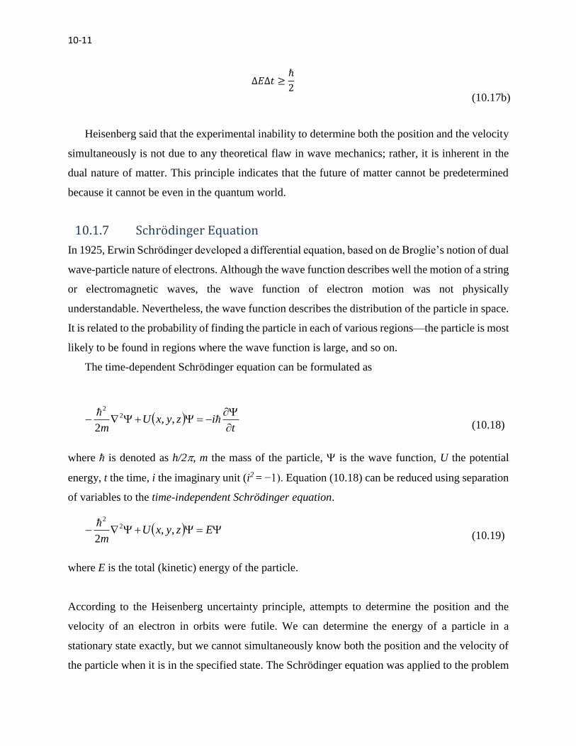
Δ𝐸Δ𝑡 ≥
ℏ
2
(10.17b)
Heisenberg said that the experimental inability to determine both the position and the velocity
simultaneously is not due to any theoretical flaw in wave mechanics; rather, it is inherent in the
dual nature of matter. This principle indicates that the future of matter cannot be predetermined
because it cannot be even in the quantum world.
10.1.7 Schrödinger Equation
In 1925, Erwin Schrödinger developed a differential equation, based on de Broglie’s notion of dual
wave-particle nature of electrons. Although the wave function describes well the motion of a string
or electromagnetic waves, the wave function of electron motion was not physically
understandable. Nevertheless, the wave function describes the distribution of the particle in space.
It is related to the probability of finding the particle in each of various regions—the particle is most
likely to be found in regions where the wave function is large, and so on.
The time-dependent Schrödinger equation can be formulated as
t
izyxUm
,,
2
22
(10.18)
where ħ is denoted as h/2, m the mass of the particle, is the wave function, U the potential
energy, t the time, i the imaginary unit (i2 = −1). Equation (10.18) can be reduced using separation
of variables to the time-independent Schrödinger equation.
EzyxUm
,,2
22
(10.19)
where E is the total (kinetic) energy of the particle.
According to the Heisenberg uncertainty principle, attempts to determine the position and the
velocity of an electron in orbits were futile. We can determine the energy of a particle in a
stationary state exactly, but we cannot simultaneously know both the position and the velocity of
the particle when it is in the specified state. The Schrödinger equation was applied to the problem

10-12
of a hydrogen atom. The solutions have quantized values on energy and angular momentum. We
recall that angular momentum quantization was put into the Bohr model as an ad hoc assumption
with no fundamental justification; with the Schrodinger equation it comes out automatically. The
predicted energy levels turned out to be identical to those from the Bohr model and thus to agree
with experimental values from spectrum analysis.
The use of wave mechanics has been limited by the difficulty of solving the Schrödinger
equation for large atoms. For a system consisting of a single electron and nucleus for a hydrogen
atom or a hydrogen-like ion, the Schrodinger equation can be solved exactly.
10.1.8 A Particle in a 1-D Box
Consider a particle in a one-dimensional box, the simplest problem for which the Schrödinger
equation with no potential energy can be solved exactly. This is schematically shown in Figure
10.7. We begin by considering a particle moving freely in one dimension with classical momentum
p. Such a particle is associated with a wave of wavelength = h/p, which is de Broglie’s formula
of Equation (10.16).
Figure 10.7 A particle in a one-dimensional box
The general wave function is deduced from Equation (10.19) with U = 0.
08
2
2
2
2
h
mE
dx
d
(10.20)
The general solution for Equation (10.20) is known to be
kxBkxAx cossin (10.21)
The wave function is bounded at the walls (x = 0 and x = L):
x=0 x=L

10-13
00 L (10.22)
Therefore, for the first boundary condition with x = 0,
00cos0sin0 BkBkA (10.23)
For the second boundary condition with x = L,
0sin kLAL (10.24)
This can be true only if
nkL ,.....3,2,1n (10.25)
Therefore, the solution of the wave function should be
xL
nAx
sin ,.....3,2,1n
(10.26)
The wave function gives the distribution of the particle that is the probability where it is likely to
be. For the total probability of finding the particle somewhere in the box to be unity,
L
dxx0
2 1
(10.27)
Substituting Equation (10.26) into (10.27), we have
L
dxxL
nA
0
22 1sin
(10.28)
The integration part is obtained as

10-14
L L
Ldx
xL
n
dxxL
n
0 0
2
22
2cos1
sin
(10.29)
Thus, combining the above two equations, we find the coefficient A as
L
A2
(10.30)
The wave function is then
xL
n
Lx
sin
2 ,.....3,2,1n
(10.31)
To find the energy En for a particle with wave function n, calculate the second derivative.
xL
nx
L
n
LL
nx
L
n
Ldx
d
dx
d
22
2
2
2
2
sin2
sin2
(10.32)
By comparing this with Equation (10.30), we obtain
2
22
8mL
nhEn ,.....3,2,1n
(10.33)
This solution of the Schrödinger equation demonstrates that a particle in a box is quantized. An
energy En and a wave function n(x) correspond to each quantum number n. These are the only
allowed stationary states of the particle in the box.
The solution to the wave equation for a particle in a box of length L provided an important test
of quantum mechanics and served to convince scientists of its validity, which is shown in Figure
10.8. The first three quantized energy levels are shown in Figure 10.8(a), the first three wave
functions in Figure 10.8(b), and the first three probability of the particle in Figure 10.8(c). Even
more importantly, the information derived from studying the wave functions for the hydrogen atom
is used to describe and predict the behavior of electrons in many-electron atoms.

10-15
Figure 10.8 (a) The potential energy for a particle in a box of length L, (b) Wave function, and
(c) The probability.
The probability of free electrons was actually observed using the scanning tunneling microscopy
[2]. The STM can be used to manipulate individual atoms on a surface. An example is shown in
Figure 10.9, where the STM tip is used to construct a “quantum corral” by pushing Fe atoms on a
Cu (111) surface into a ring. The Fe atoms scatter the surface state electrons, confining them to
the interior of the corral. The rings in the corral are the density distribution of the electrons in the
three quantum states of the corral that lie close to the Fermi energy. The atoms were imaged and
moved into position by a low-temperature, ultra-high vacuum scanning tunneling microscope.
Figure 10.9 A “quantum corral” of mean radius 7.1 nm was formed by moving 48 Fe atoms on a
Cu surface. (Image courtesy of D. M. Eigler, IBM Research Division.) (from Kittel, 2005,
Wiley)

10-16
10.1.9 Quantum Numbers
A complete theoretical treatment of a hydrogen atom, using a wave equation, yields a set of wave
functions, each described by four quantum numbers: n, l, ml, and ms. Each set of the first three (n,
l, ml) identifies quantum states of the atom, in which the electron has energy equal to En. Each
quantum state can hold no more than two electrons, which must have opposite spins. This is called
the Pauli Exclusion Principle. The fourth quantum number, ms, accounts for these opposite spins,
allowing at most two electrons in each quantum state. The fourth quantum number does not appear
when the Schrödinger equation is solved. However, the theory of relativity requires four quantum
numbers. The first three quantum numbers are associated with three-dimensional space, while the
fourth quantum number is related to time. Orbitals, states, and electrons allowed for a given shell
(n) can be obtained in the following steps:
Principal quantum number, n. The principal quantum number determines the sizes of the orbitals
and the allowed energy of the electron, having only the values ,.....3,2,1n . The principal
quantum number specifies shells. Sometimes these shells are designated by the letters K, L, M, N,
and so on. The energy obtained using the quantum mechanics for one-electron atoms is exactly the
same as Equation (10.12) that Bohr had obtained, namely
222
0
42
8 hn
meZE e
n
,.....3,2,1n (10.34)
Angular quantum number, l. The angular quantum number is associated with the shapes of the
orbitals (subshell). The allowed values of l are 0, 1, …, (n − 1) for a given value of n.
If n = 1, l can be only be 0.
If n = 2, l can be 0 or 1.
If n = 3, l can be 0, 1, or 2 and so on.
The letter assigned, respectively, to the l values 0, 1, 2, and 3 are denoted by the orbitals as s,
p, d, and f.
l 0 1 2 3
Orbital s p d f
10-17
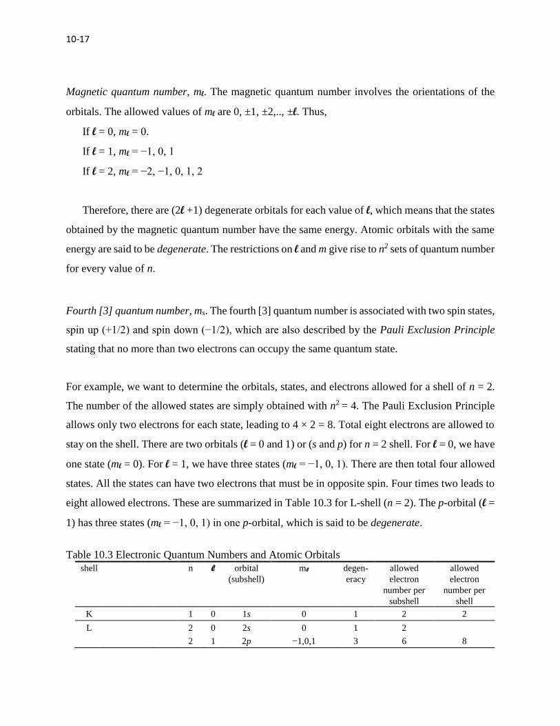
Magnetic quantum number, ml. The magnetic quantum number involves the orientations of the
orbitals. The allowed values of ml are 0, ±1, ±2,.., ±l. Thus,
If l = 0, ml = 0.
If l = 1, ml = −1, 0, 1
If l = 2, ml = −2, −1, 0, 1, 2
Therefore, there are (2l +1) degenerate orbitals for each value of l, which means that the states
obtained by the magnetic quantum number have the same energy. Atomic orbitals with the same
energy are said to be degenerate. The restrictions on l and m give rise to n2 sets of quantum number
for every value of n.
Fourth [3] quantum number, ms. The fourth [3] quantum number is associated with two spin states,
spin up (+1/2) and spin down (−1/2), which are also described by the Pauli Exclusion Principle
stating that no more than two electrons can occupy the same quantum state.
For example, we want to determine the orbitals, states, and electrons allowed for a shell of n = 2.
The number of the allowed states are simply obtained with n2 = 4. The Pauli Exclusion Principle
allows only two electrons for each state, leading to 4 × 2 = 8. Total eight electrons are allowed to
stay on the shell. There are two orbitals (l = 0 and 1) or (s and p) for n = 2 shell. For l = 0, we have
one state (ml = 0). For l = 1, we have three states (ml = −1, 0, 1). There are then total four allowed
states. All the states can have two electrons that must be in opposite spin. Four times two leads to
eight allowed electrons. These are summarized in Table 10.3 for L-shell (n = 2). The p-orbital (l =
1) has three states (ml = −1, 0, 1) in one p-orbital, which is said to be degenerate.
Table 10.3 Electronic Quantum Numbers and Atomic Orbitals
shell n l orbital
(subshell)
ml degen-
eracy
allowed
electron
number per
subshell
allowed
electron
number per
shell
K 1 0 1s 0 1 2 2
L 2 0 2s 0 1 2
2 1 2p −1,0,1 3 6 8

10-18
M 3 0 3s 0 1 2
3 1 3p −1,0,1 3 6
3 2 3d −2, −1,0,1,2 5 10 18
N 4 0 4s 0 1 2
4 1 4p −1,0,1 3 6
4 2 4d −2, −1,0,1,2 5 10
4 3 4f −3, −2,
−1,0,1,2,3
7 14 32
10.1.10 Electron Configurations
Electron configuration is the distribution of electrons in the orbitals of the atom. Electron
configuration was first conceived of under the Bohr model of the atom, and it is still common to
speak of shells and subshells, despite the advances in understanding of the quantum-mechanical
nature of electrons. The electron configurations for hydrogen, helium, and sodium are,
respectively, 1s1, 1s2, 1s22s22p63s1, where the number in front of orbital letters denotes the
principal quantum number n and the superscript of the letters denotes the number of occupied
electrons. The electron configuration associated with the lowest energy level of the atom is referred
to as ground state. Ground state electron configurations for some of the more common elements
are listed in Table 10.4. The valence electrons are those that occupy the outermost unfilled shell.
These electrons are extremely important—as will be seen, they participate in the bonding between
atoms to form atomic and molecular aggregates. Furthermore, many of the physical and chemical
properties of solids are based on these valence electrons.
We now consider a somewhat more complicated atom. The nucleus of a silicon atom contains
14 positive charges. Consequently, 14 electrons will locate themselves around this nucleus. If we
add the electrons one by one, the first 2 electrons, having opposite spin, will come to rest in the 1s
shell (n = 1) that it would be most difficult to tear away from the nucleus. The Pauli Exclusion
Principle forbids any more electrons in the first shell and dictates that the next 2 electrons will
come to rest in the 2s shell, while the next 6 electrons occupy the 2p shell with magnetic quantum
numbers −1, 0, 1 and spin quantum numbers of -½, ½. Because the energy levels specified by the
magnetic and spin quantum numbers are very close together, we show it as one energy level with
6 electrons. The next 2 electrons go into the 3s shell, while the last 2 electrons come to rest in the
3p shell. The 3s and 3p shells are valence electrons, which occupy the outermost filled shell.
Finally, the electron configuration of the silicon is 1s22s22p63s23p2.

10-19
Table 10.4 Ground State Electron Configurations for Some of the Common Elements
Atomic
Element Symbol Number Electron Configuration
Hydrogen H 1 1s1
Helium He 2 1s2
Lithium Li 3 1s22s1
Beryllium Be 4 1s22s2
Boron B 5 1s22s22p1
Carbon C 6 1s22s22p2
Nitrogen N 7 1s2 2s2 2p3
Oxygen O 8 1s22s22p4
Fluorine F 9 1s22s22p5
Neon Ne 10 1s22s22p6
Sodium Na 11 1s2 2s2 2p6 3s1
Magnesium Mg 12 1s2 2s2 2p6 3s2
Aluminum Al 13 1s2 2s2 2p6 3s2 3p1
Silicon Si 14 1s2 2s2 2p6 3s2 3p2
Phosphorus P 15 1s2 2s2 2p6 3s2 3p3
Sulfur S 16 1s2 2s2 2p6 3s2 3p4
Chlorine Cl 17 1s2 2s2 2p6 3s2 3p5
Argon Ar 18 1s2 2s2 2p6 3s2 3p6
Potassium K 19 1s2 2s2 2p6 3s2 3p64s1
Calcium Ca 20 1s2 2s2 2p6 3s2 3p6 4s2
Scandium Sc 21 1s2 2s2 2p6 3s2 3p6 3d14s2
Titanium Ti 22 1s2 2s2 2p6 3s2 3p6 3d24s2
Vanadium V 23 1s2 2s2 2p6 3s2 3p6 3d34s2
Chromium Cr 24 1s2 2s2 2p6 3s2 3p6 3d54s1
Manganese Mn 25 1s2 2s2 2p6 3s2 3p6 3d54s2
Iron Fe 26 1s2 2s2 2p6 3s2 3p6 3d64s2
Cobalt Co 27 1s2 2s2 2p6 3s2 3p6 3d74s2
Nickel Ni 28 1s2 2s2 2p6 3s2 3p6 3d84s2
Copper Cu 29 1s2 2s2 2p6 3s2 3p6 3d104s1
Zinc Zn 30 1s2 2s2 2p6 3s2 3p6 3d104s2
Gallium Ga 31 1s2 2s2 2p6 3s2 3p6 3d104s2 4p1
Germanium Ge 32 1s2 2s2 2p6 3s2 3p6 3d104s2 4p2
Arsenic As 33 1s2 2s2 2p6 3s2 3p6 3d104s2 4p3
Selenium Se 34 1s2 2s2 2p6 3s2 3p6 3d104s2 4p4
Bromine Br 35 1s2 2s2 2p6 3s2 3p6 3d104s2 4p5
Krypton Kr 36 1s2 2s2 2p6 3s2 3p6 3d104s2 4p6

10-20
Example 10.1 Electronic Configuration of a Silicon Atom
Consider a silicon atom whose atomic number is fourteen (Z = 14). Construct the electronic
configuration of the silicon atom and sketch the atomic structure indicating the orbitals (subshells)
with electrons occupied.
Solution:
We want to use Table 10.3 to figure out the electronic configuration for a silicon atom having Z =
14. First of all, we know that there are 14 electrons in a silicon atom. We find from Table 10.4 that
two electrons are allowed in K-shell (n = 1), eight electrons in L-shell (n = 2), and eighteen
electrons in M-shell (n = 3). However, since ten electrons occupy the K- and M-shell, the
remaining four electrons out of eighteen allowed electrons can only occupy the M-shell. So we
construct the electron configuration for the silicon atom according to Table 10.3 as
1s22s22p63s23p2, where the number in front of orbital letters denotes the principal quantum number
n and the superscript of the letters denotes the number of occupied electrons. If we sum the
superscript numbers as 2 + 2 + 6 + 2 + 2 = 14, the 14 indicates a total number of electrons occupied
in shells. The L-shell (n = 2) consists of two subshells and the M-shell (n = 3) also consists of two
subshells. It is noted that the energy levels specified by the angular quantum numbers (l: s and p
subshells) are very close together, we show them as one group in Figure 10.10.
Figure 10.10 A silicon atom with quantum numbers and shells
10-21
10.2 Band Theory and Doping
10.2.1 Covalent Bonding
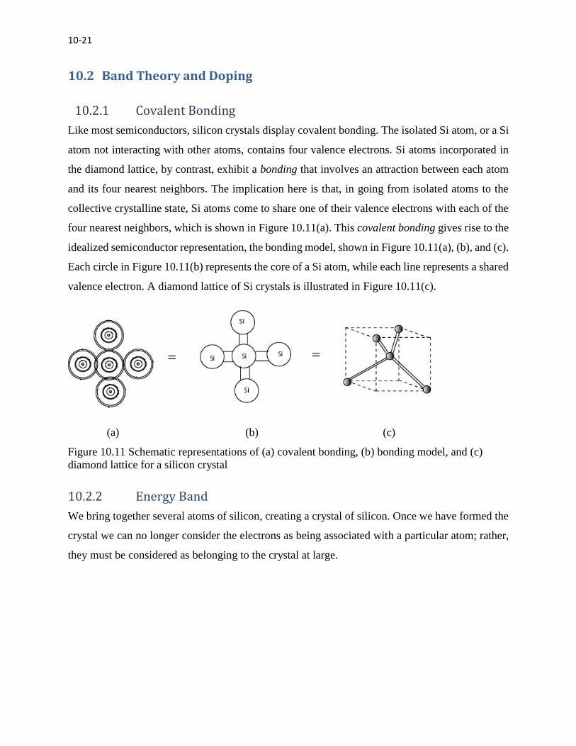
Like most semiconductors, silicon crystals display covalent bonding. The isolated Si atom, or a Si
atom not interacting with other atoms, contains four valence electrons. Si atoms incorporated in
the diamond lattice, by contrast, exhibit a bonding that involves an attraction between each atom
and its four nearest neighbors. The implication here is that, in going from isolated atoms to the
collective crystalline state, Si atoms come to share one of their valence electrons with each of the
four nearest neighbors, which is shown in Figure 10.11(a). This covalent bonding gives rise to the
idealized semiconductor representation, the bonding model, shown in Figure 10.11(a), (b), and (c).
Each circle in Figure 10.11(b) represents the core of a Si atom, while each line represents a shared
valence electron. A diamond lattice of Si crystals is illustrated in Figure 10.11(c).
(a) (b) (c)
Figure 10.11 Schematic representations of (a) covalent bonding, (b) bonding model, and (c)
diamond lattice for a silicon crystal
10.2.2 Energy Band
We bring together several atoms of silicon, creating a crystal of silicon. Once we have formed the
crystal we can no longer consider the electrons as being associated with a particular atom; rather,
they must be considered as belonging to the crystal at large.
10-22
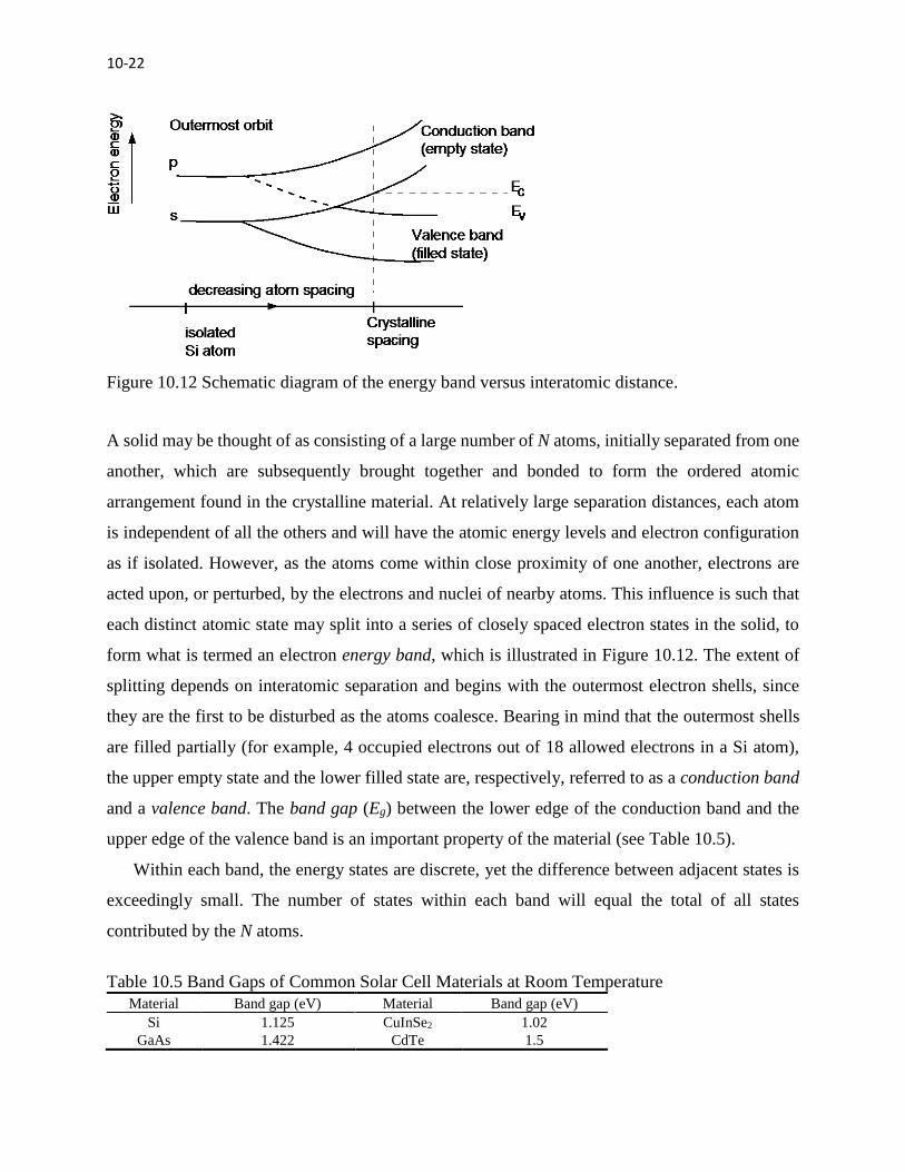
Figure 10.12 Schematic diagram of the energy band versus interatomic distance.
A solid may be thought of as consisting of a large number of N atoms, initially separated from one
another, which are subsequently brought together and bonded to form the ordered atomic
arrangement found in the crystalline material. At relatively large separation distances, each atom
is independent of all the others and will have the atomic energy levels and electron configuration
as if isolated. However, as the atoms come within close proximity of one another, electrons are
acted upon, or perturbed, by the electrons and nuclei of nearby atoms. This influence is such that
each distinct atomic state may split into a series of closely spaced electron states in the solid, to
form what is termed an electron energy band, which is illustrated in Figure 10.12. The extent of
splitting depends on interatomic separation and begins with the outermost electron shells, since
they are the first to be disturbed as the atoms coalesce. Bearing in mind that the outermost shells
are filled partially (for example, 4 occupied electrons out of 18 allowed electrons in a Si atom),
the upper empty state and the lower filled state are, respectively, referred to as a conduction band
and a valence band. The band gap (Eg) between the lower edge of the conduction band and the
upper edge of the valence band is an important property of the material (see Table 10.5).
Within each band, the energy states are discrete, yet the difference between adjacent states is
exceedingly small. The number of states within each band will equal the total of all states
contributed by the N atoms.
Table 10.5 Band Gaps of Common Solar Cell Materials at Room Temperature
Material Band gap (eV) Material Band gap (eV)
Si 1.125 CuInSe2 1.02
GaAs 1.422 CdTe 1.5

10-23
Ge 0.663
10.2.3 Pseudo-Potential Well
When an electron in a valence band receives sufficient energy by a perturbation such as
photons, an electric field, or thermal energy, the electron may jump up to the conduction band.
The electron is no longer restricted to the single atom, becoming able to freely migrate in the sea
of the conduction band. A free electron in a conduction band may be considered to be in a pool or
pseudo-potential well—actually, in a crystal. According to quantum mechanics, the free electron
is allowed to stay only in one of the allowed states (quantized energy). Therefore, the first step is
to determine how many states per unit volume are allowed in the pool, which is called the density
of states. The simplified model of energy band in a crystal is illustrated in Figure 10.13, where the
lower edge of the conduction band and the upper edge of the valence band are indicated. The free
electron in a crystal has a physical similarity with a particle in a one-dimensional box in Section
10.2.7. Accordingly, the solutions in the section can be applied to this problem.
Figure 10.13 Visualization of a conduction band electron moving in a crystal.
10.2.4 Doping, Donors, and Acceptors
Doping is a process of intentionally introducing impurities into an extremely pure (also referred to
as intrinsic) semiconductor to change its electrical properties. Some impurities, or dopants, are
generally added initially as a crystal ingot is grown, giving each wafer (a thin slice of
10-24
semiconducting material) an almost uniform initial doping. Further doping can be carried out by
such processes as diffusion or ion implantation, the latter method being more popular in large
production runs due to its better controllability. The ion implantation is a process whereby a
focused beam of ions (dopants) is directed towards a target wafer. The ions have enough kinetic
energy that they can penetrate into the wafer upon impact.
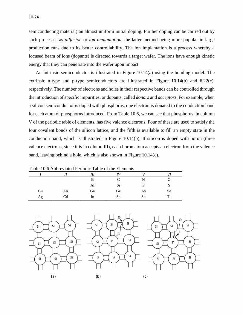
An intrinsic semiconductor is illustrated in Figure 10.14(a) using the bonding model. The
extrinsic n-type and p-type semiconductors are illustrated in Figure 10.14(b) and 6.22(c),
respectively. The number of electrons and holes in their respective bands can be controlled through
the introduction of specific impurities, or dopants, called donors and acceptors. For example, when
a silicon semiconductor is doped with phosphorus, one electron is donated to the conduction band
for each atom of phosphorus introduced. From Table 10.6, we can see that phosphorus, in column
V of the periodic table of elements, has five valence electrons. Four of these are used to satisfy the
four covalent bonds of the silicon lattice, and the fifth is available to fill an empty state in the
conduction band, which is illustrated in Figure 10.14(b). If silicon is doped with boron (three
valence electrons, since it is in column III), each boron atom accepts an electron from the valence
band, leaving behind a hole, which is also shown in Figure 10.14(c).
Table 10.6 Abbreviated Periodic Table of the Elements
I II III IV V VI
B C N O
Al Si P S
Cu Zn Ga Ge As Se
Ag Cd In Sn Sb Te
(a) (b) (c)

10-25
Figure 10.14 Visualization of (a) an intrinsic silicon bonding model, (b) a phosphorus atom
(donor) is substituted for a silicon atom, and (c) a boron atom (acceptor) is substituted for a
silicon atom, displayed using the bonding model.
The unbounded electrons of donors and the unbounded holes of acceptors are very susceptible and
are easily excited to produce free (ionized) electrons and holes, even with a thermal energy at room
temperature. A donor (phosphorus) in Figure 10.14(b) yields a negatively charged electron and the
donor itself becomes a positive charge (because of losing a negative electron from a neutral state).
An acceptor [4] yields a positively charged hole and the acceptor itself becomes a negative charge
(called ionized donor). The positively charged donors and negatively charged acceptors are
immobile due to the covalent bonding with silicon atoms and thus create an electrostatic potential,
which is called a built-in voltage. As a result, the doping directly creates a built-in voltage between
the n-type material and p-type material.
Problems
10.1 Consider that we receive some line spectra from an unknown object in the sky, some of
which are 0.434 nm, 0.486nm, and 656nm. Determine the element that composes the
object and show your detailed calculation indicating the initial and final quantum
numbers for each line spectrum.
10.2 Consider a copper atom whose atomic number is twenty-nine (Z = 29). Construct the
electronic configuration of the atom and sketch the atomic structure indicating the
orbitals (subshells) with electrons occupied.
10.3 Consider a selenium atom whose atomic number is thirty-four (Z = 34). Construct the
electronic configuration of the atom and sketch the atomic structure indicating the
orbitals (subshells) with electrons occupied.
References
1. Finn, J.W., et al., An Integrated child safety seat cooling system-model and test. IEEE Transactions on Vehicular Technology, 2012. 61(5): p. 1999-2007.
2. Chi, H., et al., Low-temperature transport properties of Tl-doped Bi_{2}Te_{3} single crystals. Physical Review B, 2013. 88(4).
3. Bubnova, O., et al., Optimization of the thermoelectric figure of merit in the conducting polymer poly(3,4-ethylenedioxythiophene). Nat Mater, 2011. 10(6): p. 429-33.

10-26
4. Farahi, N., et al., Sb- and Bi-doped Mg2Si: location of the dopants, micro- and nanostructures, electronic structures and thermoelectric properties. Dalton Trans, 2014. 43(40): p. 14983-91.