1

Chapter 10 – Confidence Intervals (CI’s) Lesson Objectives: In this chapter you will learn how to estimate the mean of an entire population. Remember, you cannot gather information from every member of the population, so you collect information about a portion of the population (you take a sample). If you collected your data appropriately (SRS) and took a large sample size the sample should adequately represent the population. You could then use that sample to estimate the population mean.

Date Topics Objectives: Students will be able to: Homework

Mar 21

10.1 The Idea of a Confidence Interval, Interpreting Confidence Levels and Confidence Intervals, Constructing a Confidence Interval

• Interpret a confidence level. • Interpret a confidence interval in context. • Understand that a confidence interval gives a

range of plausible values for the parameter.

Read Section

10.1; Watch Video #1

Mar 21

10.1 Using Confidence Intervals Wisely, 8.2 Conditions for Estimating p, Constructing a Confidence Interval for p

• Understand why each of the three inference conditions—Random, Normal, and Independent—is important.

• Explain how practical issues like nonresponse, undercoverage, and response bias can affect the interpretation of a confidence interval.

• Construct and interpret a confidence interval for a population proportion.

• Determine critical values for calculating a confidence interval using a table or your calculator.

Read Section

10.1; Watch Video #2

Mar 22

10.2 Putting It All Together: The Four-Step Process, Choosing the Sample Size

• Carry out the steps in constructing a confidence interval for a population proportion: define the parameter; check conditions; perform calculations; interpret results in context.

• Determine the sample size required to obtain a level C confidence interval for a population proportion with a specified margin of error.

• Understand how the margin of error of a confidence interval changes with the sample size and the level of confidence C.

• Understand why each of the three inference conditions—Random, Normal, and Independent—is important.

Read Section

10.2; Watch Video #2

Mar 23

8.3 When 𝜎 Is Known: The One-Sample z Interval for a Population Mean, When 𝜎 Is Unknown: The t Distributions, Constructing a Confidence Interval for 𝜇

• Construct and interpret a confidence interval for a population mean.

• Determine the sample size required to obtain a level C confidence interval for a population mean with a specified margin of error.

• Carry out the steps in constructing a confidence interval for a population mean: define the parameter; check conditions; perform calculations; interpret results in context.

Read Section

10.3; Watch Videos #

3 - 8

Mar 26

10.3 Using t Procedures Wisely Chapter 8 Review

• Understand why each of the three inference conditions—Random, Normal, and Independent—is important.

• Determine sample statistics from a confidence interval.

Chapter 8 Packet Due March 26

2

8.1 – Introduction to Confidence Intervals [VIDEO #1]

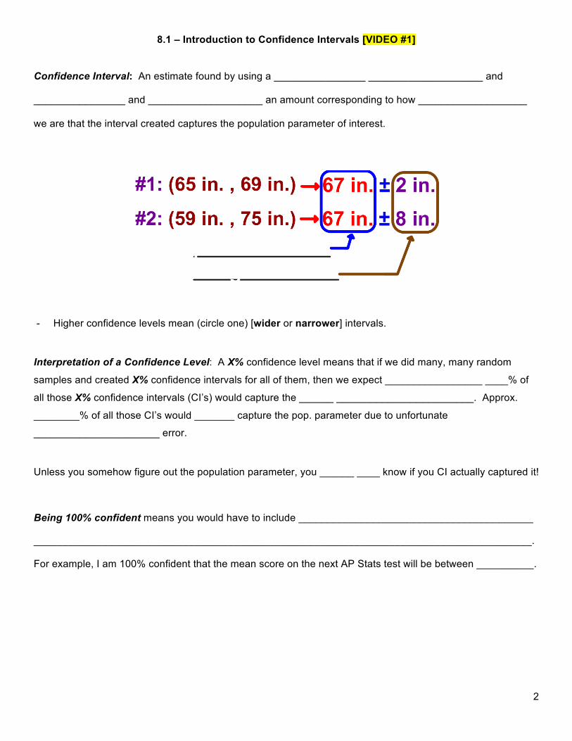
Confidence Interval: An estimate found by using a ________________ ____________________ and

________________ and ____________________ an amount corresponding to how ___________________

we are that the interval created captures the population parameter of interest.

- Higher confidence levels mean (circle one) [wider or narrower] intervals.

Interpretation of a Confidence Level: A X% confidence level means that if we did many, many random

samples and created X% confidence intervals for all of them, then we expect _________________ ____% of

all those X% confidence intervals (CI’s) would capture the ______ ________________________. Approx.

________% of all those CI’s would _______ capture the pop. parameter due to unfortunate

______________________ error.

Unless you somehow figure out the population parameter, you ______ ____ know if you CI actually captured it!

Being 100% confident means you would have to include _________________________________________

_______________________________________________________________________________________.

For example, I am 100% confident that the mean score on the next AP Stats test will be between __________.

3

8.1 – Interpretation of Confidence Intervals

Examples of “sampling error” committed during a random sample:

1. ___________________________________ 2. _________________________________________

• Using the confidence interval applet, did a 95% CI

always capture 95% of 100 generated CI’s? à

Confidence Interval Interpretations – The Good, The Bad, and The Ugly!

- The Good:

1. I am 95% confident that the mean __________ for all __________ is between _______ and _______. 2. After taking many SRS of size ____ from the population of interest, 95% of the constructed intervals

can be expected to have captured the true population parameter value. NOTE: You do not know whether a 95% CI calculated from a particular set of data contains the true parameter value.

3. I am 95% confident that the true population parameter falls within this interval.

4. The CI was calculated using a method that will capture the true population parameter in 95% of all

possible samples. - The Bad and the Ugly:

1. 95% of all California HS seniors have a SAT math score between 452 and 470. 2. The probability is 95% that the true mean falls between 452 and 470.

3. There is a 95% chance that the true mean falls in the interval.

4. 95% of the time the mean SAT score for all HS Seniors will be between 452 and 470.

REMEMBER: The population parameter we hope to estimate is a _____________ ____________. We can

only hope (with certain confidence) that our _______________ represented the population well and we

captured the _______________________ _____________________.

SAT Score HS Seniors

4

Can you tell “The Good” apart from “The Bad and the Ugly”? Mark the two statements that are correct. You have measured the amount of time spent sleeping in a day for a random sample of 25 dogs. A 95% confidence interval for the mean sleep time for the dogs is (8, 12). Which of the following statements gives a valid interpretation of this interval? a. 95% of the sample of dogs sleep between 8 and 12 hours a day. b. 95% of the population of all dogs sleep between 8 and 12 hours a day c. If the procedure were repeated many times, 95% of the resulting confidence intervals would contain the

population mean daily sleep time. d. The probability that the population mean sleep time is between 8 and 12 is 0.95. e. If the procedure were repeated many times, 95% of the sample means would be between 8 and 12 hours. f. I am 95% confident that the mean daily sleep time for all dogs is between 8 and 12 hours. g. There is a 95% probability that µ is between 8 and 12. h. If we took many, many additional random samples and from each computed a 95% confidence interval for

µ, approximately 95% of these intervals would contain µ. i. If we took many, many additional random samples and from each computed a 95% confidence interval for

µ, 95% of them would cover the values from 8 to 12. j. There is a 95% probability that the true average sleep time is between 8 and 12 hours for all dogs.

“Interpretation of 95% Confident” Questions on the 2002 and 2007 AP Exams:

2002 Question: A simple random sample produces a sample mean, x , of 15. A 95% confidence interval for the corresponding population mean is 15 ± 3. Which of the following statements must be true?

(A) Ninety-five percent of the population measurements fall between 12 and 18. (B) Nintey-five percent of the sample measurements fall between 12 and 18. (C) If 100 samples were taken, 95 of the sample means would fall between 12 and 18. (D) P(12 ≤ x ≤ 18) = 0.95 (E) If µ = 19, this x of 15 would be unlikely to occur.

2007 Question: A planning board in Elm County is interested in estimating the proportion of its residents that are in favor of offering incentives to high-tech industries to build plants in that county. A random sample of Elm County residents was selected. All of the selected residents were asked, “Are you in favor of offering incentives to high-tech industries to build plants in your county?” A 95% confidence interval for the proportion of residents in favor of offering incentives was calculated to be 0.54 ± 0.05. Which of the following statements is correct?

(A) At the 95% confidence level, the estimate of 0.54 is within 0.05 of the true proportion of county residents in favor of offering incentives to high-tech industries to build plants in the county.

(B) At the 95% confidence level, the majority of area residents are in favor of offering incentives to high-tech industries to build plants in the county.

(C) In repeated sampling, 95% of sample proportions will fall in the interval (0.49, 0.59) (D) In repeated sampling, the true proportion of county residents in favor of offering incentive to high-tech

industries to build plants in the county will fall in the interval (0.49, 0.59) (E) In repeated sampling, 95% of the time the true proportion of county residents in favor of offering

incentives to high-tech industries to build plants in the county will be equal to 0.54.

5

8.1 – Using Confidence Intervals Wisely [VIDEO #2]

You are going to be writing quite a bit of what you see in this video. You SHOULD be writing out all the conditions and checking them in the first place when working problems, so get used to the increase of writing!!!

Three (3) Conditions for using Confidence Intervals

Condition #1: ___________________________ (now write everything else on the page!!!)

Condition #2: ____________________________

Condition #3: ____________________________

6

8.2 – Introduction to CI’s for one proportion [VIDEO #3]

Earlier, we discussed about the definition of a confidence interval being a point estimator (a statistic, 𝑥 or 𝑝) plus or minus a margin of error related to how confident we were about capturing the population parameter of interest (µ or p). The formal definition is this:

___________________ ± (________________________)·(________________________________________) The part after the plus/minus is our margin of error that can be broken down into two parts. The “critical value” is related to the “how confident” we want to be with our interval while the “standard error of the statistic” is just our standard deviation for the sampling distribution of 𝑥 or 𝑝 we used last chapter.

Confidence Interval for One Proportion

Statistic ± (Critical Value)(Standard Error of the Statistic) Turns specifically into…

p̂ ± nppz )ˆ1(ˆ* −

Conditions: 1. The data must come from a __________________________________ from the population of interest.

a. YOU MUST WRITE BEFORE DOING ANY CALCULATIONS: “We have a SRS of (size/#)

(people or whatever you sampled) to represent ALL (people or whatever you sampled).

b. If there is no mention of a random sample, then write “Sample not known to be random,

proceed with caution!” and continue with the problem.

2. The observations of your sample must be _____________________________.

a. Check the “10%” condition a.k.a. “Population > 10·n”. SHOW YOUR WORK!

If it checks, then write “We may proceed to calculate the standard error.”

b. If NOT, then you need to use the Finite Population Correction formula we mentioned before but

will not use in this class, so write “Standard error cannot be safely calculated.” STOP.

3. The sampling distribution of 𝑝 must be _____________________ ________________________.

a. Check the condition n ·> 𝑝 10 and n(1 - 𝑝) > 10. SHOW THE ACTUAL WORK HERE!

If it checks, then write “We may assume the sampling distribution is approx. normal.”

b. If NOT, then write “Sampling distribution not normal, CI cannot be calculated.” STOP.

c. NOTE: The CLT does NOT work with proportion problems, so don’t use it here!!!

7

8.2 – z* (Critical Values) [VIDEO #3 cont.]

The 68-95-99.7 rule or the Empirical rule is an approximation.

Confidence Level Drawing Tail Area z* = “Critical Value”

68

90

95

99

99.7

C

8

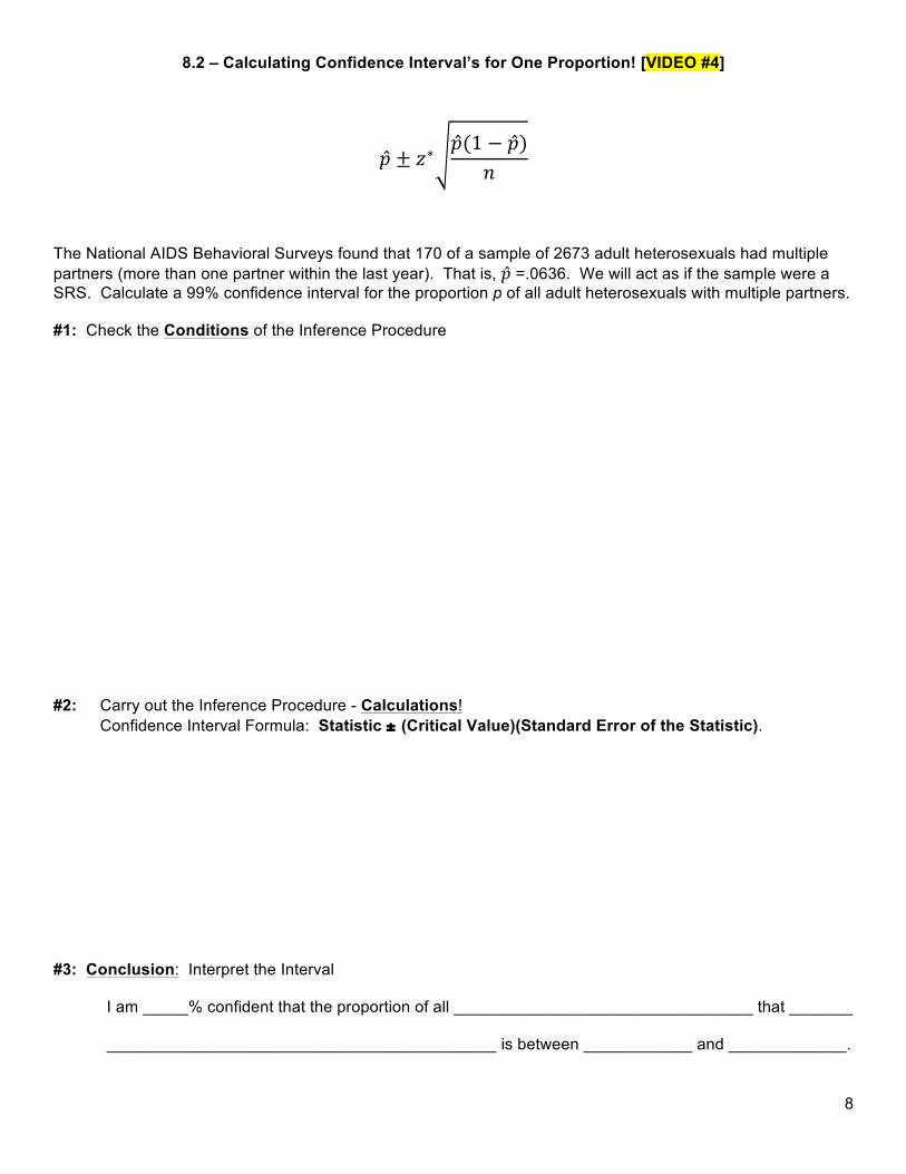
8.2 – Calculating Confidence Interval’s for One Proportion! [VIDEO #4]

𝑝 ± 𝑧∗𝑝(1 − 𝑝)

𝑛

The National AIDS Behavioral Surveys found that 170 of a sample of 2673 adult heterosexuals had multiple partners (more than one partner within the last year). That is, 𝑝 =.0636. We will act as if the sample were a SRS. Calculate a 99% confidence interval for the proportion p of all adult heterosexuals with multiple partners. #1: Check the Conditions of the Inference Procedure #2: Carry out the Inference Procedure - Calculations!

Confidence Interval Formula: Statistic ± (Critical Value)(Standard Error of the Statistic).

#3: Conclusion: Interpret the Interval

I am _____% confident that the proportion of all _________________________________ that _______

___________________________________________ is between ____________ and _____________.

9

8.2 - Choosing the Sample Size [VIDEO #5] In planning a study, we may want to choose a sample size that will allow us to estimate the parameter within a given margin of error.

𝑚 = 𝑧∗𝑝(1 − 𝑝)

𝑛

Problem: Until we actually do the study we won’t know what 𝑝 is. We need to guess approximately What 𝑝 will be. We will call this guess p*.

Remedy #1: Guess p* based on past experience Remedy #2: Use p* = .5. The margin of error is largest when 𝑝= .5, so this guess is conservative in

the sense that if we get any other 𝑝 value when we do our study, we will get a margin of error smaller than planned. Use p* = .5 when you expect the true value of p to be roughly between .3 and .7

Finding Sample Size Gloria Chavez and Ronald Flynn are candidates for mayor in a large city. You are planning a sample survey to determine what percent of the voters plan to vote for Chavez. You will contact a SRS of registered voters in the city. You want to estimate p with 95% confidence and a margin of error no greater than 3%, or .03. How large of a sample do you need?

10

8.3 – Introduction to CI’s for One Mean & t Distributions [VIDEO #6]

When we seek to capture the population mean, 𝜇 , by using a sample mean, 𝑥, with a CI, chances are we do NOT know the population standard deviation, 𝜎. IF you somehow happen to know, 𝜎 then use the formula:

𝑥 ± 𝑧∗𝜎𝑛

In reality, σ is not known (if you knew σ you would also know µ and have no need to estimate it).

a. What do we use to estimate µ? _________

b. What do we use to estimate σ? _________

c. Rather than use 𝜎! =𝜎𝑛 , what will the new formula become? ___________________

d. When the standard deviation is estimated from the data, the formula !!

is no longer called standard

deviation of the statistic, but rather the ___________________________ of the statistic, abbreviated

“SEM”

When we use “s” in place of “σ”, the statistic that results does not have a normal distribution. It has a new

distribution called a ______________________. t-statistics are used and interpreted the same way as a z-

statistic, but there is a different t distribution for each sample size. We specify a particular t distribution by

giving its _______________________, which is ____________.

So this à 𝑥 ± 𝑧∗ !!

turns into this à 𝑥 ± 𝑡∗ !!

Describing the t distribution: The density curves of the t distribution are similar in shape to the _________________________.

S: As the degrees of freedom (n-1) ____________, the t distribution

approaches the ___________________ curve ever more closely.

Why does this happen? ________________________________

O: There should be few outliers, if any.

C: They are centered at __________, just like normal curves.

S: The spread of the t distributions are _______________________

that of the standard normal distribution. Why?

____________________________________________________

Table B (in the back of the book) gives critical values for the t distributions.

11

You also have the t-distribution values in the back of your formula sheet. Practice Problems:

1. The scores of four roommates on the Law School Aptitude Test have mean 𝑥 = 589 and standard deviation s = 37. What is the standard error of the mean?

2. What critical value t* from Table B satisfies each of the following conditions?

a. The t distribution with 10 degrees of freedom and has probability 0.01 to the right of t*. b. The t distribution with 28 degrees of freedom and has probability 0.90 to the left of t*. c. The one-sample t statistic from a sample of 42 observations that has probability 0.05 to the right of t*. d. The one-sample t statistic from a SRS of 980 observations and has probability 0.975 to the left. e. A 95% CI based on a SRS of 15 observations. f. A 99% CI from a sample size of 110 observations. g. A 90% CI based on 30 observations.

12

8.3 – Calculating CI’s for One Mean [VIDEO #7]

Confidence Interval for One Mean

Statistic ± (Critical Value)(Standard Error of the Statistic) Turns specifically into…

𝑥 ± 𝑡∗𝑠𝑛

Conditions: 1. The data must come from a __________________________________ from the population of interest.

a. YOU MUST WRITE BEFORE DOING ANY CALCULATIONS: “We have a SRS of (size/#)

(people or whatever you sampled) to represent ALL (people or whatever you sampled).

b. If there is no mention of a random sample, then write “Sample not known to be random,

proceed with caution!” and continue with the problem.

2. The observations of your sample must be _____________________________.

a. Check the “10%” condition a.k.a. “Population > 10·n”. SHOW YOUR WORK!

If it checks, then write “We may proceed to calculate the standard error.”

b. If NOT, then you need to use the Finite Population Correction formula we mentioned before but

will not use in this class, so write “Standard error cannot be safely calculated.” STOP.

3. The sampling distribution of 𝑥 must be _____________________ ________________________.

a. If you know σ somehow, then you can say and use the normal distribution (z-scores).

If you do not know σ, then you can saw and use the t-distribution (t-scores). (More likely)

b. If the population is known to be Normal (REGARDLESS OF SAMPLE SIZE), then write “Since

the population is known to be normal, then we may assume the sampling distribution can

follow an (select one: approx. normal or t) distribution.”

c. If NOT, then check for a sufficiently large enough sample size (> 30) for the CLT to apply

If so, write “Sampling distribution can use t-procedures due to the CLT and sample size.”

d. If sample size is less than 30: t procedures can be used except in the presence of outliers or

strong skewness (some skewness OK). Plot your data (stemplot or boxplot) to check for

Normality (roughly symmetric, single peak, no outliers). If the data checks out, then write

“Based on the data shown, we may assume a t-distribution with ___ df.”

e. If the data are STRONGLY skewed or if outliers are present, do not use t. STOP.

13

Ex 1: A company manufactures portable music devices—called “mBoxes”—for the listening pleasure of on-the-go teens. The mBox uses batteries that are advertised to provide, on average, 25 hours of continuous use. The students in Mr. Jones’s statistics class—looking for any excuse to listen to music while doing their homework—decide to use their statistics to test this advertising claim. To do this, new batteries are installed in eight randomly selected mBoxes, and they are used only in Mr. Jones’s class until the batteries run down. Here are the results for the lifetimes of the batteries (in hours):

15 22 26 25 21 27 18 22

Construct and interpret a 95% CI for the mean number of hours (µ) that the batteries can be expected to last. C: Check the Conditions of the Inference Procedure C: Carry out the Inference Procedure - Calculations!

Confidence Interval Formula: Statistic ± (Critical Value)(Standard Error of the Statistic).

𝑥 ± 𝑡∗ !!

C: Conclusion: Interpret the Interval

I am _____% confident that the mean _____________________ for all __________________ is

between ____________ and _____________.

14

8.3 – Calculating a Confidence Interval for a Mean Difference (Matched Pairs) [VIDEO #8] Examples of Matched Pairs Experimental Designs: 1. Two seeds of the same type of plant are planted in the same pot. One is randomly selected and treated

with a new fertilizer. The other seed serves as the control. We want to estimate the mean difference in growth for 10 such pairs of plants.

2. An elementary school teacher uses a matched pairs design when giving a pretest and posttest and then determining if the students improved.

3. A study tries to determine whether caffeine addicts are more depressed when they receive a “caffeine placebo” rather than a “caffeine pill”.

What makes an experimental design “Matched Pairs”? _______________________________________

___________________________________________________________________________________

How do you analyze a matched pairs data set? _____________________________________________

___________________________________________________________________________________

Matched Pairs Procedure Example: Our subjects are 11 people diagnosed as being dependent on caffeine. Each subject was barred from coffee, colas, and other substances containing caffeine. Instead, they took capsules containing their normal caffeine intake. During a different time period, they took placebo capsules. The order in which subjects took caffeine and the placebo was randomized. One of the tests given to the subjects was “Depression” as scored by the Beck Depression Inventory. Higher scores show more symptoms of depression. Construct and interpret a 90% confidence interval for the mean change in depression score.

• Conditions:

• Calculations:

• Conclusion:

15

Upon completion of Chapter 10, you should be able to. . . q Find a z* value for any confidence level (for the calculation of a CI) using Table A or on your calculator.

For example, what z* corresponds to 82% confidence? q Find the required sample size needed to obtain a specific margin of error. PS – To do this you need to

know the formula for margin of error. q Interpret a given confidence interval. If we took many SRS and calculated CI’s about 95% of them would

capture the true population parameter (5% of them would miss the population parameter) q Explain how a change in the sample size or confidence level affects the length of a CI. q Construct and Interpret a 90%, 95%, or 99% CI for a given data set or for given information. q Make sure you know your formulas and don’t get the components of them mixed up. You should know

them off by heart from doing HW problems. q Check the conditions for each procedure, including the fact that outliers and/or strong skewness invalidate t

procedure results q Calculate the standard error of the mean q Find t* with either Table B or on your calculator. q The difference between a one sample t and a matched pairs t procedure q Verify that the population is normal with either a stemplot, histogram, or boxplot, be sure to note the

absence of outliers and strong skewness q Calculate the standard error for a one sample proportion. q Find the necessary sample size for a specific margin of error or confidence interval length (A CI of length .5

has a margin of error of .25) q Calculate a confidence interval for a one sample proportion for any specified confidence level