Chapter 10 Magic Squares - MathWorks · PDF file2 Chapter 10. Magic Squares course, we do not have any eye-witness accounts, so we can only imagine that the turtle looked like ﬁgure

Chapter 10

Magic Squares

With origins in centuries old recreational mathematics, magic squares demonstrateMatlab array operations.

Figure 10.1. Lo Shu. (Thanks to Byerly Wiser Cline.)

Magic squares predate recorded history. An ancient Chinese legend tells of aturtle emerging from the Lo river during a flood. The turtle’s shell showed a veryunusual pattern – a three-by-three grid containing various numbers of spots. Of

Copyright c⃝ 2011 Cleve MolerMatlabR⃝ is a registered trademark of MathWorks, Inc.TM

October 2, 2011

1

2 Chapter 10. Magic Squares

course, we do not have any eye-witness accounts, so we can only imagine that theturtle looked like figure 10.1. Each of the three rows, the three columns, and thetwo diagonals contain a total of 15 spots. References to Lo Shu and the Lo Shunumerical pattern occur throughout Chinese history. Today, it is the mathematicalbasis for Feng Shui, the philosophy of balance and harmony in our surroundingsand lives.

An n-by-n magic square is an array containing the integers from 1 to n2,arranged so that each of the rows, each of the columns, and the two principaldiagonals have the same sum. For each n > 2, there are many different magicsquares of order n, but the Matlab function magic(n) generates a particular one.

Matlab can generate Lo Shu with

A = magic(3)

which produces

A =

8 1 6

3 5 7

4 9 2

The command

sum(A)

sums the elements in each column to produce

15 15 15

The command

sum(A’)’

transposes the matrix, sums the columns of the transpose, and then transposes theresults to produce the row sums

15

15

15

The command

sum(diag(A))

sums the main diagonal of A, which runs from upper left to lower right, to produce

15

The opposite diagonal, which runs from upper right to lower left, is less importantin linear algebra, so finding its sum is a little trickier. One way to do it makes useof the function that “flips” a matrix “upside-down.”

3

sum(diag(flipud(A)))

produces

15

This verifies that A has equal row, column, and diagonal sums.Why is the magic sum equal to 15? The command

sum(1:9)

tells us that the sum of the integers from 1 to 9 is 45. If these integers are allocatedto 3 columns with equal sums, that sum must be

sum(1:9)/3

which is 15.There are eight possible ways to place a transparency on an overhead projec-

tor. Similarly, there are eight magic squares of order three that are rotations andreflections of A. The statements

for k = 0:3

rot90(A,k)

rot90(A’,k)

end

display all eight of them.

8 1 6 8 3 4

3 5 7 1 5 9

4 9 2 6 7 2

6 7 2 4 9 2

1 5 9 3 5 7

8 3 4 8 1 6

2 9 4 2 7 6

7 5 3 9 5 1

6 1 8 4 3 8

4 3 8 6 1 8

9 5 1 7 5 3

2 7 6 2 9 4

These are all the magic squares of order three. The 5 is always in the center, theother odd numbers are always in the centers of the edges, and the even numbersare always in the corners.

Melancholia I is a famous Renaissance engraving by the German artist andamateur mathematician Albrecht Durer. It shows many mathematical objects, in-cluding a sphere, a truncated rhombohedron, and, in the upper right hand corner,a magic square of order 4. You can see the engraving in our figure 10.2. Better yet,issue these Matlab commands


..

Figure 10.2. Albrect Durer’s Melancolia, 1514.

load durer

whos

You will see

X 648x509 2638656 double array

caption 2x28 112 char array

map 128x3 3072 double array

The elements of the array X are indices into the gray-scale color map named map.The image is displayed with

image(X)

colormap(map)

axis image

Click the magnifying glass with a “+” in the toolbar and use the mouse to zoomin on the magic square in the upper right-hand corner. The scanning resolutionbecomes evident as you zoom in. The commands

load detail

5

..

Figure 10.3. Detail from Melancolia.

image(X)

colormap(map)

axis image

display the higher resolution scan of the area around the magic square that we havein figure 10.3.

The command

A = magic(4)

produces a 4-by-4 magic square.

A =

16 2 3 13

5 11 10 8

9 7 6 12

4 14 15 1

The commands

sum(A), sum(A’), sum(diag(A)), sum(diag(flipud(A)))

yield enough 34’s to verify that A is indeed a magic square.The 4-by-4 magic square generated by Matlab is not the same as Durer’s

magic square. We need to interchange the second and third columns.

A = A(:,[1 3 2 4])


changes A to

A =

16 3 2 13

5 10 11 8

9 6 7 12

4 15 14 1

Interchanging columns does not change the column sums or the row sums. It usuallychanges the diagonal sums, but in this case both diagonal sums are still 34. So nowour magic square matches the one in Durer’s etching. Durer probably chose thisparticular 4-by-4 square because the date he did the work, 1514, occurs in themiddle of the bottom row.

The program durerperm interchanges rows and columns in the image producedfrom detail by interchanging groups of rows and columns in the array X. This isnot especially important or useful, but it provides an interesting exercise.

We have seen two different 4-by-4 magic squares. It turns out that there are880 different magic squares of order 4 and 275305224 different magic squares oforder 5. Determining the number of different magic squares of order 6 or larger isan unsolved mathematical problem.

For a magic square of order n, the magic sum is

µ(n) =1

n

n2∑k=1

k

which turns out to be

µ(n) =n3 + n

2.

Here is the beginning of a table of values of the magic sum.

n µ(n)3 154 345 656 1117 1758 260

You can compute µ(n) in Matlab with either

sum(diag(magic(n)))

or

(n^3 + n)/2

The algorithms for generating matrix square fall into three distinct cases:

7

odd, n is odd.singly-even, n is divisible by 2, but not by 4.doubly-even, n is divisible by 4.

The best known algorithm for generating magic squares of odd order is de LaLoubere’s method. Simon de La Loubere was the French ambassador to Siam in thelate 17th century. I sometimes refer to his method as the ”nor’easter algorithm”,after the winter storms that move northeasterly up the coast of New England. Youcan see why if you follow the integers sequentially through magic(9).

47 58 69 80 1 12 23 34 45

57 68 79 9 11 22 33 44 46

67 78 8 10 21 32 43 54 56

77 7 18 20 31 42 53 55 66

6 17 19 30 41 52 63 65 76

16 27 29 40 51 62 64 75 5

26 28 39 50 61 72 74 4 15

36 38 49 60 71 73 3 14 25

37 48 59 70 81 2 13 24 35

The integers from 1 to n2 are inserted along diagonals, starting in the middleof first row and heading in a northeasterly direction. When you go off an edge of thearray, which you do at the very first step, continue from the opposite edge. Whenyou bump into a cell that is already occupied, drop down one row and continue.

We used this algorithm in Matlab for many years. Here is the code.

A = zeros(n,n);

i = 1;

j = (n+1)/2;

for k = 1:n^2

is = i;

js = j;

A(i,j) = k;

i = n - rem(n+1-i,n);

j = rem(j,n) + 1;

if A(i,j) ~= 0

i = rem(is,n) + 1;

j = js;

end

end

A big difficulty with this algorithm and resulting program is that it insertsthe elements one at a time – it cannot be vectorized.

A few years ago we discovered an algorithm for generating the same magicsquares of odd order as de La Loubere’s method, but with just four Matlab matrixoperations.

[I,J] = ndgrid(1:n);


A = mod(I+J+(n-3)/2,n);

B = mod(I+2*J-2,n);

M = n*A + B + 1;

Let’s see how this works with n = 5. The statement

[I,J] = ndgrid(1:n)

produces a pair of matrices whose elements are just the row and column indices, iand j.

I =

1 1 1 1 1

2 2 2 2 2

3 3 3 3 3

4 4 4 4 4

5 5 5 5 5

J =

1 2 3 4 5

1 2 3 4 5

1 2 3 4 5

1 2 3 4 5

1 2 3 4 5

Using these indices, we generate two more matrices. The statements

A = mod(I+J+1,n)

B = mod(I+2*J-2,n)

produce

A =

3 4 0 1 2

4 0 1 2 3

0 1 2 3 4

1 2 3 4 0

2 3 4 0 1

B =

1 3 0 2 4

2 4 1 3 0

3 0 2 4 1

4 1 3 0 2

0 2 4 1 3

Both A and B are fledgling magic squares. They have equal row, column and diagonalsums. But their elements are not the integers from 1 to n2. Each has duplicatedelements between 0 and n− 1. The final statement

9

M = n*A+B+1

produces a matrix whose elements are integers between 1 and n2 and which hasequal row, column and diagonal sums. What is not obvious, but is true, is thatthere are no duplicates. So M must contain all of the integers between 1 and n2 andconsequently is a magic square.

M =

17 24 1 8 15

23 5 7 14 16

4 6 13 20 22

10 12 19 21 3

11 18 25 2 9

The doubly-even algorithm is also short and sweet, and tricky.

M = reshape(1:n^2,n,n)’;


K = fix(mod(I,4)/2) == fix(mod(J,4)/2);

M(K) = n^2+1 - M(K);

Let’s look at our friend magic(4). The matrix M is initially just the integersfrom 1 to 16 stored sequentially in 4 rows.

M =

1 2 3 4

5 6 7 8

9 10 11 12

13 14 15 16

The logical array K is true for half of the indices and false for the other half in apattern like this.

K =

1 0 0 1

0 1 1 0

0 1 1 0

1 0 0 1

The elements where K is false, that is 0, are left alone.

. 2 3 .

5 . . 8

9 . . 12

. 14 15 .

The elements where K is true, that is 1, are reversed.

16 . . 13

. 11 10 .

. 7 6 .

4 . . 1


The final result merges these two matrices to produce the magic square.The algorithm for singly even order is the most complicated and so we will give

just a glimpse of how it works. If n is singly even, then n/2 is odd and magic(n)

can be constructed from four copies of magic(n/2). For example, magic(10) isobtained from A = magic(5) by forming a block matrix.

[ A A+50

A+75 A+25 ]

The column sums are all equal because sum(A) + sum(A+75) equals sum(A+50) + sum(A+25).But the rows sums are not quite right. The algorithm must finish by doing a fewswaps of pieces of rows to clean up the row sums. For the details, issue the com-mand.

type magic

9 10

11 12

Figure 10.4. Surf plots of magic squares of order 9, 10, 11,12.

Let’s conclude this chapter with some graphics. Figure 10.4 shows

surf(magic(9)) surf(magic(10))

surf(magic(11)) surf(magic(12))

You can see the three different cases – on the left, the upper right, and the lowerright. If you increase of each of the orders by 4, you get more cells, but the globalshapes remain the same. The odd n case on the left reminds me of Origami.

11

Further ReadingThe reasons why Matlab has magic squares can be traced back to my junior highschool days when I discovered a classic book by W. W. Rouse Ball, MathematicalRecreations and Essays. Ball lived from 1850 until 1925. He was a fellow of TrinityCollege, Cambridge. The first edition of his book on mathematical recreationswas published in 1892 and the tenth edition in 1937. Later editions were revisedand updated by another famous mathematician, H. S. M Coxeter. The thirteenthedition, published by Dover in 1987, is available from many booksellers, includingPowells and Amazon.

http://www.powells.com/cgi-bin/biblio?inkey=17-0486253570-0

http://www.amazon.com/Mathematical-Recreations-Essays-Dover-Books/

dp/0486253570

There are dozens of interesting Web pages about magic squares. Here are a fewauthors and links to their pages.

Mutsumi Suzukihttp://mathforum.org/te/exchange/hosted/suzuki/MagicSquare.html

Eric Weissteinhttp://mathworld.wolfram.com/MagicSquare.html

Kwon Young Shinhttp://user.chollian.net/~brainstm/MagicSquare.htm

Walter Trumphttp://www.trump.de/magic-squares

Recap%% Magic Squares Chapter Recap

% This is an executable program that illustrates the statements

% introduced in the Magic Squares Chapter of "Experiments in MATLAB".

% You can access it with

%

% magic_recap

% edit magic_recap

% publish magic_recap

%

% Related EXM programs

%

% magic

% ismagical

%% A Few Elementary Array Operations.

format short

A = magic(3)

sum(A)


sum(A’)’

sum(diag(A))

sum(diag(flipud(A)))

sum(1:9)/3

for k = 0:3

rot90(A,k)

rot90(A’,k)

end

%% Durer’s Melancolia

clear all

close all

figure

load durer

whos

image(X)

colormap(map)

axis image

%% Durer’s Magic Square

figure

load detail

image(X)

colormap(map)

axis image

A = magic(4)

A = A(:,[1 3 2 4])

%% Magic Sum

n = (3:10)’;

(n.^3 + n)/2

%% Odd Order

n = 5


A = mod(I+J+(n-3)/2,n);

B = mod(I+2*J-2,n);

M = n*A + B + 1

%% Doubly Even Order

n = 4

M = reshape(1:n^2,n,n)’;


K = fix(mod(I,4)/2) == fix(mod(J,4)/2);

M(K) = n^2+1 - M(K)

13

%% Rank

figure

for n = 3:20

r(n) = rank(magic(n));

end

bar(r)

axis([2 21 0 20])

%% Ismagical

help ismagical

for n = 3:10

ismagical(magic(n))

end

%% Surf Plots

figure

for n = 9:12

subplot(2,2,n-8)

surf(rot90(magic(n)))

axis tight off

text(0,0,20,num2str(n))

end

set(gcf,’color’,’white’)

Exercises

10.1 ismagic. Write a Matlab function ismagic(A) that checks if A is a magicsquare.

10.2 Magic sum. Show that

1

n

n2∑k=1

k =n3 + n

2.

10.3 durerperm. Investigate the durerperm program. Click on two different elementsto interchange rows and columns. Do the interchanges preserve row and columnsums? Do the interchanges preserve the diagonal sums?

10.4 Colormaps. Try this.

clear

load detail

whos


You will see three matrices in your workspace. You can look at all of map andcaption.

map

caption

The matrix X is 359-by-371. That’s 133189 elements. Look at just a piece of it.

X(101:130,101:118)

The elements of X are integers in the range

min(min(X))

max(max(X))

The commands

image(X)

axis image

produce a pretty colorful display. That’s because the elements of X are being usedas indices into the default colormap, jet(64). You can use the intended colormapinstead.

colormap(map)

The array map is a 64-by-3 array. Each row, map(k,:), specifies intensities of red,green and blue. The color used at point (i,j) is map(X(i,j),:). In this case, thecolormap that comes with detail has all three columns equal to each other and sois the same as

colormap(gray(64))

Now experiment with other colormaps

colormap(hot)

colormap(cool)

colormap(copper)

colormap(pink)

colormap(bone)

colormap(flag)

colormap(hsv)

You can even cycle through 101 colormaps.

for p = 0:.001:1

colormap(p*hot+(1-p)*pink)

drawnow

end

You can plot the three color components of a colormap like hot with

15

rgbplot(hot)

This is what TV movie channels do when they colorize old black and white films.

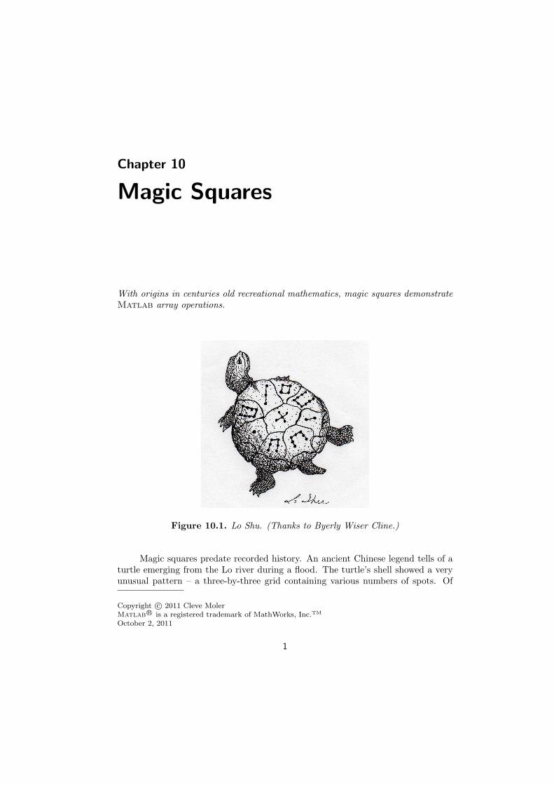
10.5 Knight’s tour. Do you know how a knight is allowed to move on a chess board?The exm function knightstour generates this matrix, K.

K =

50 11 24 63 14 37 26 35

23 62 51 12 25 34 15 38

10 49 64 21 40 13 36 27

61 22 9 52 33 28 39 16

48 7 60 1 20 41 54 29

59 4 45 8 53 32 17 42

6 47 2 57 44 19 30 55

3 58 5 46 31 56 43 18

If you follow the elements in numerical order, you will be taken on a knight’s tourof K. Even the step from 64 back to 1 is a knight’s move.Is K a magic square? Why or why not?Try this.

image(K)

colormap(pink)

axis square

Select the data cursor icon on the figure tour bar. Now use the mouse to take theknight’s tour from dark to light on the image.

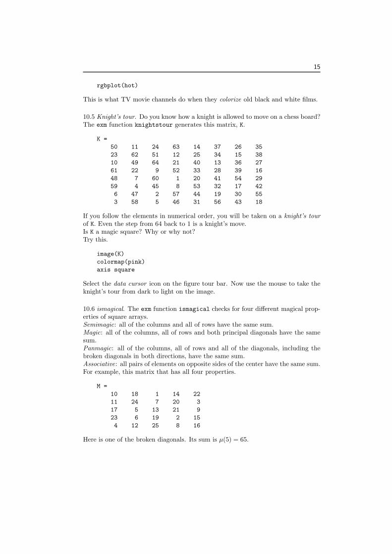
10.6 ismagical. The exm function ismagical checks for four different magical prop-erties of square arrays.Semimagic: all of the columns and all of rows have the same sum.Magic: all of the columns, all of rows and both principal diagonals have the samesum.Panmagic: all of the columns, all of rows and all of the diagonals, including thebroken diagonals in both directions, have the same sum.Associative: all pairs of elements on opposite sides of the center have the same sum.For example, this matrix that has all four properties.

M =

10 18 1 14 22

11 24 7 20 3

17 5 13 21 9

23 6 19 2 15

4 12 25 8 16

Here is one of the broken diagonals. Its sum is µ(5) = 65.


. . . 14 .

. . . . 3

17 . . . .

. 6 . . .

. . 25 . .

All of the broken diagonals in both directions have the same sum, so M is panmagic.One pair of elements on opposite sides of the center is 24 and 2. Their sum is twicethe center value. All pairs of elements on opposite sides of the center have this sum,so M is associative.(a) Use ismagical to verify that M has all four properties.(b) Use ismagical to investigate the magical properties of the matrices generatedby the Matlab magic function.(c) Use ismagical to investigate the magical properties of the matrices generatedby this algorithm for various odd n and various values of a0 and b0,

a0 = ...

b0 = ...


A = mod(I+J-a0,n);

B = mod(I+2*J-b0,n);

M = n*A + B + 1;

(d) Use ismagical to investigate the magical properties of the matrices generatedby this algorithm for various odd n and various values of a0 and b0,

a0 = ...

b0 = ...


A = mod(I+2*J-a0,n);

B = mod(I+3*J-b0,n);

M = n*A + B + 1;

10.7 Inverse. If you have studied matrix theory, you have heard of matrix inverses.What is the matrix inverse of a magic square of order n? It turns out to dependupon whether n is odd or even. For odd n, the matrices magic(n) are nonsingular.The matrices

X = inv(magic(n))

do not have positive, integer entries, but they do have equal row and column sums.But, for even n, the determinant, det(magic(n)), is 0, and the inverse does

not exist. If A = magic(4) trying to compute inv(A) produces an error message.

10.8 Rank. If you have studied matrix theory, you know that the rank of a matrix isthe number of linearly independent rows and columns. An n-by-n matrix is singularif its rank, r, is not equal to its order. This code computes the rank of the magicsquares up to order 20, generated with

17

for n = 3:20

r(n) = rank(magic(n));

end

The results are

n = 3 4 5 6 7 8 9 10 11 12 13 14 15 16 17 18 19 20

r = 3 3 5 5 7 3 9 7 11 3 13 9 15 3 17 11 19 3

Do you see the pattern? Maybe the bar graph in figure 10.5 will help. You can see

2 4 6 8 10 12 14 16 18 200

2

4

6

8

10

12

14

16

18

20

Figure 10.5. Rank of magic squares.

that the three different algorithms used to generate magic squares produce matriceswith different rank.

n rank

odd n

even, not divisible by 4 n/2+2

divisible by 4 3

Documents

Chapter 10 Magic Squares - MathWorks · PDF file2 Chapter 10. Magic Squares course, we do not have any eye-witness accounts, so we can only imagine that the turtle looked like ﬁgure