Chapter 10 - CA Sri Lanka Risk Return...10.1 A First Look at Risk and Return We begin our look at risk and return by illustrating how the risk premium affects investor decisions and

PowerPointto accompany

Chapter 10

Introduction to

Investments &

Risk and Return in

Capital Markets

Copyright © 2011 Pearson Australia (a division of Pearson Australia Group Ltd) –

9781442502000 / Berk/DeMarzo/Harford / Fundamentals of Corporate Finance / 1st edition

Investing

Purchase of assets with the goal of

increasing future income

Focuses on wealth accumulation

Underlying investment decisions: the

tradeoff between expected return and risk

Expected return is not usually the same as

realized return

Risk: the possibility that the realized return

will be different than the expected return

2



Total return on investment expressed

as a percentage of the amount of

money invested

Investments usually earn higher rates

of return than savings tools

Rate of Return

Total Return

Amount of

Money Invested

Rate of Return



Risk

Risk- uncertainty regarding the

outcome of a situation or event

Investment Risk- possibility that an

investment will fail to pay the expected

return or fail to pay a return at all

All investment tools carry some level of

risk



Types of Investment Tools

Stocks Bonds

Mutual Funds

Index Funds

Real Estate

Cash



Risk Return Tradeoff

Investors manage risk at a cost

- lower expected returns (ER)

Any level of expected return and risk

can be attained

Risk

ER

Risk-free Rate

Bonds

Stocks



10.1 A First Look at Risk and Return

We begin our look at risk and return by illustrating how the risk premium affects investor decisions and returns:

Suppose you won $10,000 in a raffle in December 1988 and decided to invest it all in a portfolio of Australian shares, with dividends being reinvested.

By December 2008, 20 years later, your shareportfolio would be worth $55,695 and a comparable portfolio of cash $41,134 as shown in Figure 10.1.

The impact of the stock market decline of 2007 and the global slowdown that occurred from 2008 is evident in the sharp decline of the graph.

7



Figure 10.1 Value of $10,000 Invested in Cash and Australian Shares over 20 Years from December 1988

8



Table 10.1 Range of Returns on Australian Investments over 20 Years from December 1988

9

The table above shows returns of four investment classes with different risk profiles over 20 years.

The general principle is that investors do not like risk and demand a premium to bear it.



Individual investment realised return

The realised return is the total return that occurs

over a particular time period.

The realised return from your investment from t

to t+1 is:

(Eq. 10.1)

10

FORMULA!

10.2 Historical Risks and Returns of Securities



Example 10.1 Realised Return (p.314)

Problem:

Metropolis Limited paid a one-time special

dividend of $3.08 on 15 November 2010.

Suppose you bought a Metropolis share for

$28.08 on 1 November 2010 and sold it

immediately after the dividend was paid for

$27.39.

What was your realised return from holding the

share?

11



Solution:

Plan:

We can use Eq. 10.1 to calculate the realised

return.

We need the purchase price ($28.08), the selling

price ($27.39), and the dividend ($3.08) and we

are ready to proceed.

12




Execute:

Using Eq. 10.1, the return from 1 Nov 2010 until 15 Nov

2010 is equal to:

This 8.51% can be broken down into the dividend yield

and the capital gain yield:

13




Evaluate:

These returns include both the capital gain (or in this case a capital loss) and the return generated from receiving dividends.

Both dividends and capital gains contribute to the total realised return—ignoring either one would give a very misleading impression of Metropolis’ performance.

14




Individual investment realised return

For quarterly returns (or any four compounding

periods that make up an entire year), the annual

realised return, which can be observed over

years, Rannual, is found by compounding:

1+ Rannual =(1+R1) (1+R2) (1+R3) (1+R4)

(Eq. 10.2)

15


FORMULA!



Example 10.2 Compounding Realised Returns (pp.315-6)

Problem:

Suppose you purchased Metropolis shares on 1

November 2010 and held them for one year,

selling on 31 October 2011. All dividends you

earned were re-invested in the same Metropolis

shares.

What was your realised return?

16



Solution:

Plan:

We need to analyse the cash flows from holding

Metropolis shares for each quarter.

In order to get the cash flows, we must look up

Metropolis share price data at the start and end

of the year, as well as at any dividend dates.

From the data we can construct the following

table to fill out our cash flow timeline:

17




Plan (cont’d):

Next, calculate the return between each set of dates using Eq. 10.1.

Then, determine each annual return similarly to

Eq. 10.2 by compounding the returns for all of the

periods in that year.18




Execute:

In Example 10.1, we already calculated the

realised return for 1 Nov to 15 Nov 2010 as 8.51%.

We continue this for each period until we have a

series of realised returns.

For example, from 15 Nov 2010 to 15 Feb 2011,

the realised return is:

19




Execute (cont’d):

We then determine the one-year return by

compounding:

20




Execute (cont’d):

The table below includes the realised return at

each period:

21




Evaluate:

By repeating these steps, we have successfully calculated the realised annual returns for an investor holding Metropolis shares over this one-year period.

From this exercise, we can see that returns are risky.

Metropolis fluctuated up and down over the year and ended up only slightly up (2.75%) at the end.

22




Average annual returns

The average annual return of an investment during some historical period is simply the average of the realised returns for each year.

That is, if Rt is the realised return of a security in each year t, then the average annual return for years one through T is:

23


(Eq. 10.3)

FORMULA!



The average return provides a estimate of the return we should expect in any given year.

24

Table 10.2 Annual Returns on the Australian All Ordinaries Index 2004-08



The variance and volatility of returns

To determine the variability, we calculate the standard deviation of the distribution of realised returns, which is the square root of the variance of the distribution of realised returns.

Variance measures the variability in returns by taking the differences of the returns from the average return and squaring those differences.

25


FORMULA! (Eq. 10.4)



(Eq. 10.5)

26

Variance estimate using realised returns

We have to square the difference of each return

from the average, because the unsquared

differences from an average must be zero.

Because we square the returns, the variance is in

units of ‘%2’ or per cent-squared, which is not

useful.

So we take the square root, to get the standard

deviation in units of ‘%’.


FORMULA!



Example 10.3 Calculating Historical Volatility (pp.318-9)

Problem:

Using the data from Table 10.2, what is the

standard deviation of the return on the All

Ordinaries Index for the years 2004–08?

27



Solution:

Plan:

First, calculate the average return using Eq. 10.3

because it is an input to the variance equation.

Next, calculate the variance using Eq. 10.4 and

then take its square root to determine the standard

deviation.

28




Execute:

In the previous section we already calculated the

average annual return of the All Ordinaries

during this period as 9.74%, so we have all of the

necessary inputs for the variance calculation.

From Eq. 10.4, we have:

29




Execute (cont'd):

Alternatively, we can break the calculation of this

equation out as follows:

Summing the squared differences in the last row, we get 0.3531.

30




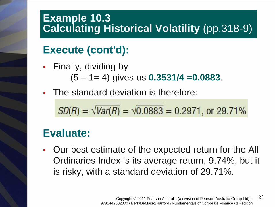
Execute (cont'd):

Finally, dividing by

(5 – 1= 4) gives us 0.3531/4 =0.0883.

The standard deviation is therefore:

Evaluate:

Our best estimate of the expected return for the All

Ordinaries Index is its average return, 9.74%, but it

is risky, with a standard deviation of 29.71%.

31




The normal distribution

Standard deviations are useful for more than just

ranking the investments from riskiest to least risky.

It also describes a normal distribution, shown in

Figure 10.2:

About two-thirds of all possible outcomes fall within

one standard deviation above or below the average.

About 95% of all possible outcomes fall within two

standard deviations above and below the average.

Figure 10.2 shows these outcomes for the shares of a

hypothetical company.

32




Figure 10.2 Normal Distribution

33

Because we are about 95% confident that next year’s

returns will be within two standard deviations of the

average:

(Eq. 10.6)



Table 10.3 Summary of Tools for Working with Historical Returns

34



The returns of large portfolios

Figure 10.3 plots the average returns versus the

volatility of US large company shares, US small

shares, US corporate bonds, US Treasury bills

and a world portfolio.

Note that investments with higher volatility,

measured by standard deviation, have rewarded

investors with higher average returns.

This is consistent with the view that investors are

risk averse—risky investments must offer higher

average returns to compensate for the risk.

35

10.3 The Historical Trade-off Between Risk and Return



Figure 10.3 The Historical Trade-off Between Risk and Return in Large Portfolios, 1926–2006

36



Returns of individual securities

The following observations are noteworthy

1. There is a relationship between size and risk—larger shares have lower volatility than smaller ones.

2. Even the largest shares are typically more volatile than a portfolio of large shares, such as the S&P 500.

3. All individual shares have lower returns and/or higher risk than the portfolios in Figure 10.3—the individual shares all lie below the line in the figure.

37




Individual securities

While volatility (standard deviation) seems to be

a reasonable measure of risk when evaluating a

large portfolio, the volatility of an individual

security doesn’t explain the size of its average

return.

38




10.4 Common versus Independent Risk

Example: Theft vs earthquake insurance

Consider two types of home insurance: theft

insurance and earthquake insurance.

Assume that the risk of each of these two hazards

is similar for a given home in Sydney. Each year

there is about a 1% chance the home will be

robbed, and also a 1% chance the home will be

damaged by an earthquake.

Suppose an insurance company writes 100,000

policies of each type of insurance for homeowners

in Sydney. Are the risks of the two portfolios of

policies similar?

39



10.4 Common versus Independent Risk

Example: Theft vs earthquake insurance

Why are the portfolios of insurance policies so

different when the individual policies themselves

are quite similar?

Intuitively, the key difference between them is that an

earthquake affects all houses simultaneously, so the

risk is linked across homes—common risk.

The risk of theft is not linked across homes, some

homeowners are unlucky, others lucky—independent

risk.

Diversification: the averaging out of independent

risk in a large portfolio.

40



Table 10.4 Summary of Types of Risk

41



Example 10.5 Diversification (p.325)

Problem:

You are playing a very simple gambling game

with your friend: a $1 bet based on a coin flip.

That is, you each bet $1 and flip a coin: heads

you win your friend’s dollar, tails you lose and

your friend takes your dollar.

How is your risk different if you play this game

100 times in a row versus just betting $100

(instead of $1) on a single coin flip?

42



Solution:

Plan:

The risk of losing one coin flip is independent of the risk of losing the next one—each time you have a 50% chance of losing, and one coin flip does not affect any other coin flip.

We can calculate the expected outcome of any flip as a weighted average by weighting your possible winnings (+$1) by 50% and your possible losses (–$1) by 50%.

We can then calculate the probability of losing all $100 under either scenario.

43




Execute:

If you play the game 100 times, you should lose

about 50% of the time and win 50% of the time,

so your expected outcome is:

50 (+$1) + 50 (–$1) = $0

You should break even.

However the probability of losing $100 is

= 0.5 x 0.5 x 0.5 ………..

= 0.5100

= 0.000000000000000000000000000078%

If it happens, you should take a very careful look

at the coin! 44




Execute (cont’d):

If, instead, you make a single $100 bet on the

outcome of one coin flip, you have a 50% chance

of winning $100 and a 50% chance of losing

$100, so your expected outcome will be the

same—break even.

However, there is a 50% chance you will lose

$100, so your risk is far greater than it would be

for 100 one dollar bets.

45




Evaluate:

In each case, you put $100 at risk, but by

spreading out that risk across 100 different bets,

you have diversified much of your risk away

compared to placing a single $100 bet.

46




10.5 Diversification in Share Portfolios

As the insurance example indicates, the risk of a

portfolio depends upon whether the individual

risks within it are common or independent.

Independent risks are diversified in a large

portfolio, whereas common risks are not.

Our goal is to understand the relation between

risk and return in the capital markets, so let’s

consider the implication of this distinction for the

risk of stock portfolios.

47



Unsystematic vs systematic risk Share prices and dividends fluctuate due to two

types of news:

Company- or industry-specific news: good or bad news about a company (or industry) itself. For example, a firm might announce that it has been successful in gaining market share within its industry.

Market-wide news: news that affects the economy as a whole and therefore affects all shares. For example, the Reserve Bank might announce that it will lower interest rates to boost the economy.

48




Unsystematic vs systematic risk

Fluctuations of a share’s return that are due to company- or industry-specific news are independent risks.

Like theft across homes, these risks are unrelated across shares and are also referred to as unsystematic risk.

On the other hand, fluctuations of a share’s return that are due to market-wide news represent common risk, which affect all shares simultaneously.

This type of risk is also called systematic risk.

49




Figure 10.4 Volatility of Portfolios of Type S and U Shares

50



Unsystematic vs systematic risk

When firms carry both types of risk, only the

unsystematic risk will be diversified away when

we combine many firms into a portfolio.

The volatility will therefore decline until only the

systematic risk, which affects all firms, remains.

51




Figure 10.5 The Effect of Diversification on Portfolio Volatility

52



Diversifiable risk and the risk premium

Competition among investors ensures that no

additional return can be earned for diversifiable

risk.

The risk premium of a share is not affected by

its diversifiable, unsystematic risk.

The risk premium for diversifiable risk is zero.

Thus, investors are not compensated for

holding unsystematic risk.

53




Table 10.5 The Expected Return of Type S and Type U Firms, Assuming the Risk-Free Rate is 5%

54

The risk premium of a security is determined by its

systematic risk and does not depend on its

diversifiable risk.



Table 10.6 Systematic Risk versus Unsystematic Risk

Thus, there is no relationship between volatility and

average returns for individual securities.

55

Documents

Chapter 10 - CA Sri Lanka Risk Return...10.1 A First Look at Risk and Return We begin our look at risk and return by illustrating how the risk premium affects investor decisions and