Chapter 1 Stochastic Programming from Modeling Languagesgondzio/CV/spfml.pdf · 2002-05-17 · i i Chapter 1 Stochastic Programming from Modeling Languages Emmanuel Fragni ere1 and

i

i

i

i

Chapter 1

Stochastic Programmingfrom Modeling Languages

Emmanuel Fragniere1 and Jacek Gondzio2

1.1 IntroductionThe majority of deterministic mathematical programming problems have a compactformulation in terms of algebraic equations. Therefore they can easily take advan-tage of the facilities offered by algebraic modeling languages. These tools allowexpressing models by using convenient mathematical notation (algebraic equations)and translate the models into a form understandable by the solvers for mathematicalprograms.

Algebraic modeling languages provide facility for the management of a math-ematical model and its data, and access different general-purpose solvers. The useof algebraic modeling languages (AMLs) simplifies the process of building the pro-totype model and in some cases makes it possible to create and maintain even theproduction version of the model.

As presented in other chapters of this book, stochastic programming (SP) isneeded when exogenous parameters of the mathematical programming problem arerandom. Dealing with stochasticities in planning is not an easy task. In a standardscenario-by-scenario analysis, the system is optimized for each scenario separately.Varying the scenario hypotheses we can observe the different optimal responses ofthe system and delineate the “strong trends” of the future. Indeed, this scenario-by-scenario approach implicitly assumes perfect foresight. The method provides afirst-stage decision, which is valid only for the scenario under consideration. Havingas many decisions as there are scenarios leaves the decision-maker without a clearrecommendation. In stochastic programming the whole set of scenarios is combinedinto an event tree, which describes the unfolding of uncertainties over the periodof planning. The model takes into account the uncertainties characterizing thescenarios through stochastic programming techniques. This adaptive plan is muchcloser, in spirit, to the way that decision-makers have to deal with uncertain future

1

i

i

i

i

2 Chapter 1. Stochastic Programming from Modeling Languages

in real life.Most of the difficulties to model uncertainty through stochastic programming

originate from the lack of an agreed standard of its representation. Indeed, stochas-tic programming problems usually involve dynamic aspects of decision making whichcombined with uncertainty inevitably leads to a complicated model. To make theproblem tractable, uncertainty is usually expressed in terms of an approximate dis-crete distribution. However, the need of accuracy in modeling inevitably leads to theexplosion of dimension in the size of the corresponding mathematical program. Thisimposes additional limits on the way of modeling stochastic programming problemsand further complicates the management of such models. In consequence there stilldoes not exist a standard way of modeling stochastic programming problems in al-gebraic modeling languages. However, AML developers are working on them andhave already come up with a number of possible extensions.

In this chapter we address the difficulties of modeling stochastic programs anddiscuss in detail different approaches developed so far to deal with this problem.

The chapter is organized as follows. In Section 1.2 we briefly explain theimportant role played by AMLs in the development of optimization based models. InSection 1.3 we present different formulations of stochastic programs. In Section 1.4we discuss specific issues related to an automatic generation of stochastic programsthat result in difficulties with standardization of their generation by AMLs. InSection 1.5 we discuss the techniques of stochastic programming available to AMLsand in Section 1.6 we comment on the crucial issues of communication betweenthe solver and the algebraic modeling language. Finally, in Section 1.7 we give ourconclusions.

1.2 Algebraic Modeling LanguagesAlgebraic Modeling Languages (AMLs for short) enable decision models to be for-mulated with an algebraic notation. They use a generic model description in formof a data file. The models developed with AMLs can be easily modified. The userbuilds the model and provides the AML with the appropriate data. The AMLtranslates the model into a form that is understandable to a solver and invokes theappropriate solver. In this setting, the solver is seen as a black box. The optimiza-tion code may query the AML about any additional information on the problem.For example, nonlinear optimization code may ask for the function values as well asthe first and the second derivatives at a given point. Once the solution of the math-ematical program is found, it is returned to the AML and the results are reportedto the user.

AML enables a modeler to express the problem in an index-based mathematicalform with abstract entities: sets, indices, parameters, variables and constraints. Thekey notion in the AML is the ability to group conceptually similar entities into a set.Once the entities are grouped in a given set, they can be referenced by indices to theelements of this set. This leads to a problem formulation that is very close to theformulation using algebraic notations. For instance, the mathematical operation∑i∈I Xi is represented by the expression SUM(I, X(I)) in the GAMS modeling

i

i

i

i

1.2. Algebraic Modeling Languages 3

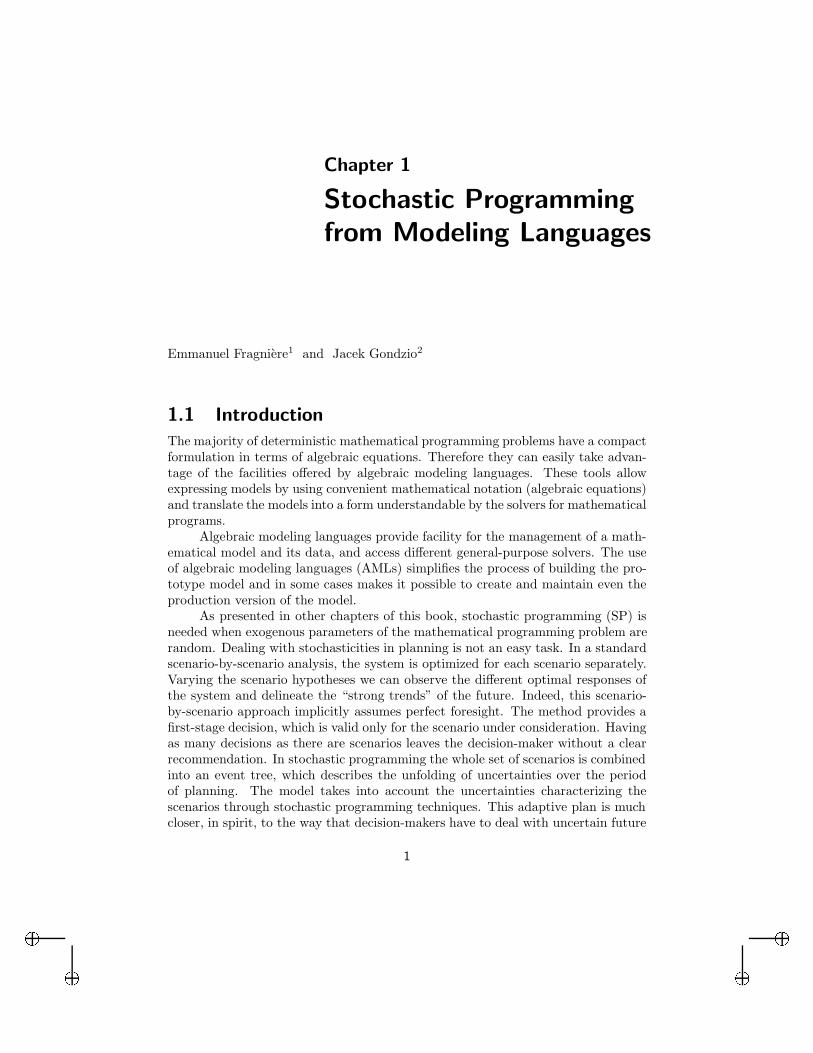
t = 1 t = 2 t = 3 t = 4 t = 5

Figure 1.1. Deterministic Invendeman model.

language. The role of the AML is to expand the compact problem formulation(problem structure and data) into the problem instance which is ready to be solvedby an appropriate optimization code. This operation is realized within the AML byreplicating every entity over the different elements of the set. This is often referredto as a set-indexing ability of the AML. The user of an AML can define genericexpressions that are indexed over several sets. Set-indexing in such cases involvescompound sets.

There exist many algebraic modeling languages or more generally, optimiza-tion modeling languages (Fragniere and Gondzio 2002). Algebraic modeling lan-guages such as GAMS (Brooke, Kendrick, and Meeraus 1992), AMPL (Fourer,Gay, and Kernighan 1993) or AIMMS (Bisschop and Entriken 1993) are routinelyused by the mathematical programming community.

To illustrate the use of such modeling tools, we first present the algebraicformulation of a multiperiod inventory model with deterministic demands. A fulldescription of this model, called Invendeman, can be found in Chapter 10 of the bookby Thompson (1992). The model has the form of a simple optimization problem:

maxT∑t=1

((pt − 2)x−t − (pt + 2)x+t − hIt)

s.t. x−t − x+t + It − It−1 = −dt

It ≤ Ix−t , x

+t , It ≥ 0.

(1.1)

The objective function corresponds to the net profit. There are three genericvariables (inventory, quantity bought, quantity sold) and one generic constraint(inventory balance), all indexed over time. A representation of a five-period instance(T = 5) is shown in Figure 1.1. The variables used in the model have the followingmeaning:

• t is the time period, t = 1, 2, ..., T ,• T is the total number of time periods,• x+

t is the quantity bought in period t,• x−t is the quantity sold in period t,• 2 is the unit transactions cost which has to be paid each time a purchase or

sale is made,• pt is the market price at time t; a seller gets pt − 2; a buyer pays pt + 2,• dt is the demand of the firm for the commodity at time t,• I0 is the initial stock of the commodity,

i

i

i

i


• It is the stock of inventory held at time t,• IT is the required final inventory of the commodity,• I is the fixed warehouse capacity,• h is the unit holding cost for inventory.

We present below an extract of the corresponding model written using theGAMS (Brooke, Kendrick, and Meeraus 1992) modeling language (the full modelalong with the data can be found in Appendix .1).

OBJECTIVE.. PROFIT =E= SUM(INDEX,(P(INDEX)-2.0)*XMINUS(INDEX)-(P(INDEX)+2.0)*XPLUS(INDEX)-H*I(INDEX-1));

INVBAL(T-1).. XMINUS(T)-XPLUS(T)+I(T)-I(T-1) =E= -D(T);

We note that the formulation in GAMS is very close to the original algebraicformulation. In general terms, algebraic modeling languages provide declarativestatements (as opposed to programming languages which contain procedural state-ments such as loops or if-then-else commands). This means that the code in thecase of an AML can be seen as a declaration of the properties of the optimizationproblem.

The modeling language takes as an input, the algebraic formulation of themodel and a set of data. Next all operations are automated. The modeling languagegenerates a mathematical program, also called an instance of the problem. Ina particular case of the deterministic multiperiod inventory model, the generatedinstance can be seen as a unique scenario. Later in this chapter we shall extend thismodel to take uncertainty into account. This will necessitate considering severalscenarios.

1.3 Different Formulations of StochasticProgramming Problems

A multistage stochastic program with recourse is a multi-period mathematical pro-gram where parameters are assumed to be uncertain along the time path. Theterm recourse means that the decision variables adapt to the different outcomes ofrandom parameters at each time period. A natural formulation of the stochasticprogramming problem relies on recursion (Birge et al. 1987) to describe dynamicsof the modeled process. Several different formulations of SPs have been discussedin detail in Part 1 of the book. Therefore we omit recursive formulations and onlybriefly mention event trees and the deterministic equivalent formulation and an al-ternative formulation with nonanticipativity constraints, two forms which are mostoften used for modeling SPs using AMLs.

1.3.1 Event Tree and the Deterministic Equivalent Formulation

In a planning approach the evolution of uncertainties can be described as an al-ternation of decisions and random realizations. In its simplest form the discretestochastic process can be represented as an event tree describing the unfolding of

i

i

i

i

1.3. Different Formulations of Stochastic Programming Problems 5

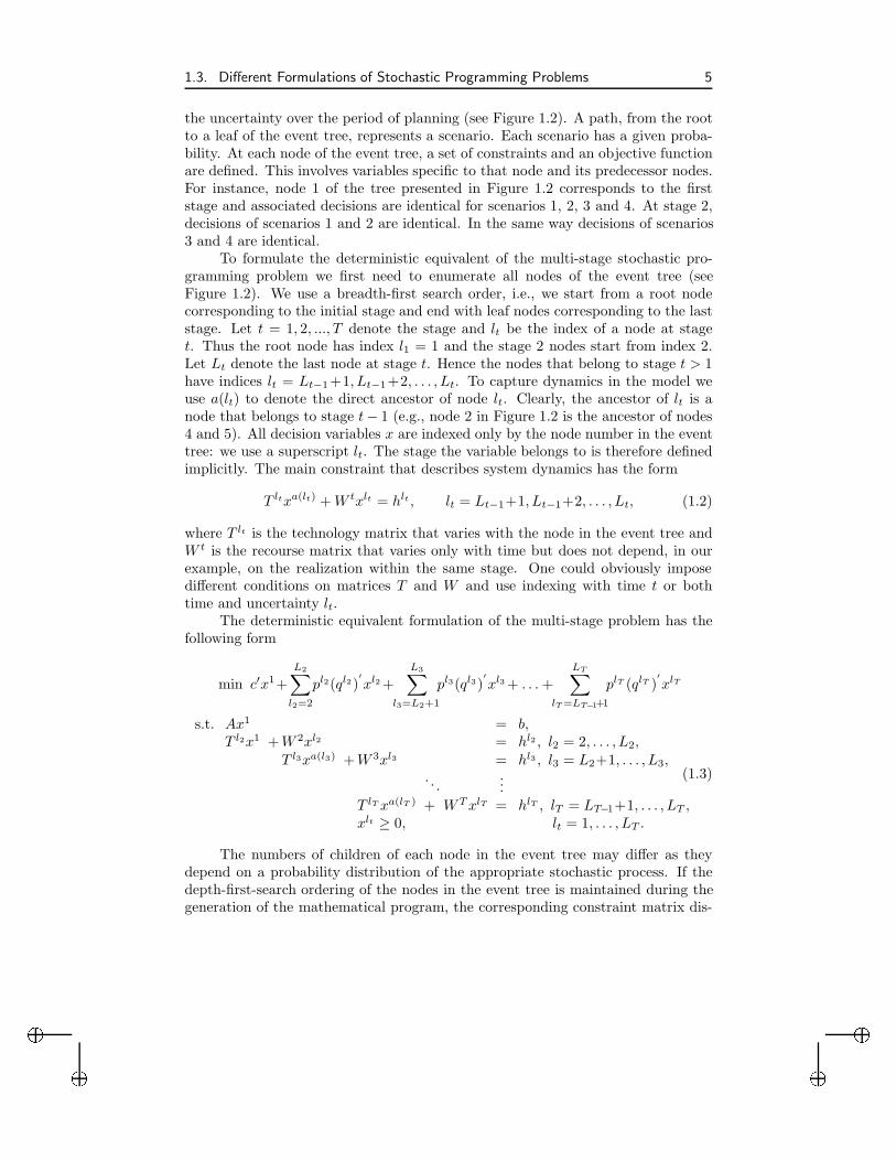
the uncertainty over the period of planning (see Figure 1.2). A path, from the rootto a leaf of the event tree, represents a scenario. Each scenario has a given proba-bility. At each node of the event tree, a set of constraints and an objective functionare defined. This involves variables specific to that node and its predecessor nodes.For instance, node 1 of the tree presented in Figure 1.2 corresponds to the firststage and associated decisions are identical for scenarios 1, 2, 3 and 4. At stage 2,decisions of scenarios 1 and 2 are identical. In the same way decisions of scenarios3 and 4 are identical.

To formulate the deterministic equivalent of the multi-stage stochastic pro-gramming problem we first need to enumerate all nodes of the event tree (seeFigure 1.2). We use a breadth-first search order, i.e., we start from a root nodecorresponding to the initial stage and end with leaf nodes corresponding to the laststage. Let t = 1, 2, ..., T denote the stage and lt be the index of a node at staget. Thus the root node has index l1 = 1 and the stage 2 nodes start from index 2.Let Lt denote the last node at stage t. Hence the nodes that belong to stage t > 1have indices lt = Lt−1 +1, Lt−1+2, . . . , Lt. To capture dynamics in the model weuse a(lt) to denote the direct ancestor of node lt. Clearly, the ancestor of lt is anode that belongs to stage t− 1 (e.g., node 2 in Figure 1.2 is the ancestor of nodes4 and 5). All decision variables x are indexed only by the node number in the eventtree: we use a superscript lt. The stage the variable belongs to is therefore definedimplicitly. The main constraint that describes system dynamics has the form

T ltxa(lt) +W txlt = hlt , lt = Lt−1+1, Lt−1+2, . . . , Lt, (1.2)

where T lt is the technology matrix that varies with the node in the event tree andW t is the recourse matrix that varies only with time but does not depend, in ourexample, on the realization within the same stage. One could obviously imposedifferent conditions on matrices T and W and use indexing with time t or bothtime and uncertainty lt.

The deterministic equivalent formulation of the multi-stage problem has thefollowing form

min c′x1+L2∑l2=2

pl2(ql2)′xl2 +

L3∑l3=L2+1

pl3(ql3)′xl3 + . . .+

LT∑lT=LT−1+1

plT (qlT )′xlT

s.t. Ax1 = b,T l2x1 +W 2xl2 = hl2 , l2 = 2, . . . , L2,

T l3xa(l3) +W 3xl3 = hl3 , l3 = L2+1, . . . , L3,. . .

...T lT xa(lT ) + WTxlT = hlT , lT = LT−1+1, . . . , LT ,xlt ≥ 0, lt = 1, . . . , LT .

(1.3)

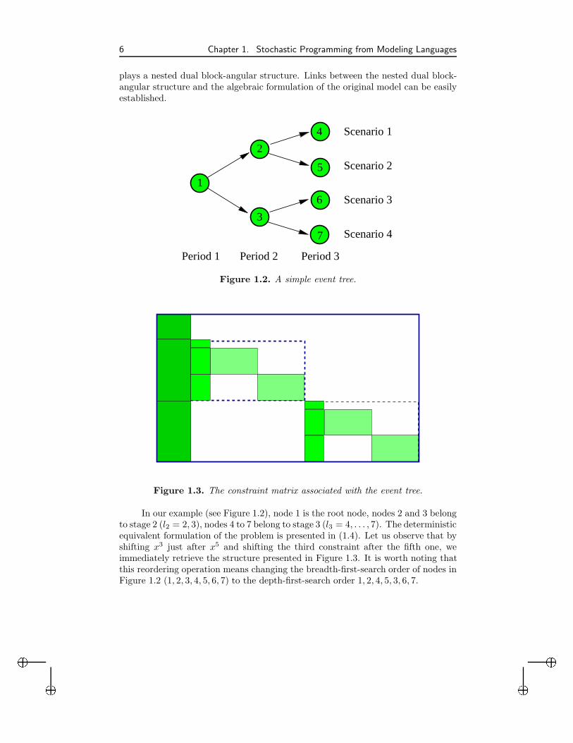
The numbers of children of each node in the event tree may differ as theydepend on a probability distribution of the appropriate stochastic process. If thedepth-first-search ordering of the nodes in the event tree is maintained during thegeneration of the mathematical program, the corresponding constraint matrix dis-

i

i

i

i


plays a nested dual block-angular structure. Links between the nested dual block-angular structure and the algebraic formulation of the original model can be easilyestablished.

1

2

3

Period 1 Period 2 Period 3

Scenario 1

Scenario 2

Scenario 3

Scenario 4

4

5

7

6

Figure 1.2. A simple event tree.

Figure 1.3. The constraint matrix associated with the event tree.

In our example (see Figure 1.2), node 1 is the root node, nodes 2 and 3 belongto stage 2 (l2 = 2, 3), nodes 4 to 7 belong to stage 3 (l3 = 4, . . . , 7). The deterministicequivalent formulation of the problem is presented in (1.4). Let us observe that byshifting x3 just after x5 and shifting the third constraint after the fifth one, weimmediately retrieve the structure presented in Figure 1.3. It is worth noting thatthis reordering operation means changing the breadth-first-search order of nodes inFigure 1.2 (1, 2, 3, 4, 5, 6, 7) to the depth-first-search order 1, 2, 4, 5, 3, 6, 7.

i

i

i

i

1.3. Different Formulations of Stochastic Programming Problems 7

min c′x1+p2(q2)′x2+p3(q3)

′x3+p4(q4)

′x4+p5(q5)

′x5+p6(q6)

′x6+p7(q7)

′x7

s.t.Ax1 = bT 2x1 + W 2x2 = h2

T 3x1 + W 2x3 = h3

T 4x2 + W 3x4 = h4

T 5x2 + W 3x5 = h5

T 6x3 + W 3x6 = h6

T 7x3 + W 3x7 = h7

x1 ≥ 0, x2 ≥ 0, x3 ≥ 0, x4 ≥ 0, x5 ≥ 0, x6 ≥ 0, x7 ≥ 0.

(1.4)

Note also that the probabilities in the objective function of problem (1.4) are notscenario probabilities but (partial) path probabilities: pn is the probability (at thestart) that a path goes through node n. Clearly, (1.4) represents a structured linearprogram. Its structure should be exploited in the solution algorithm. Unfortunately,if the model is written with an algebraic modeling language, the structure, easilyidentifiable in the algebraic formulation, is usually lost when the correspondingmathematical program is sent to the solver. Each algebraic modeling language usesits own algorithm to generate an equivalent mathematical program, which scramblesthe structure.

1.3.2 Formulation with Nonanticipativity Constraints

Another way to write the deterministic equivalent consists in creating independentcopies of variables corresponding to every ancestor in the tree for every child ofthis node. In other words, we replicate the variable xa(lt) in (1.2) and create copiesxltt−1 for each lt corresponding to a child node of a(lt) in the event tree. We slightlychange the notation at this point and add explicitly the stage subscript to eachvariable. Namely, with a given node lt at stage t we associate two variables: anappropriate decision variable xltt (at stage t) and a copy of the decision variable atthe ancestor node corresponding to this particular child, xltt−1. For example, thevariable x3 representing the state corresponding to node 3 in stage 2 in Figure 1.2would have two copies x6

2 and x72. Hence the last two constraints in (1.4) can be

replaced with the following two constraints

T 6x62 + W 3x6

3 = h6

T 7x72 + W 3x7

3 = h7

each with an independent set of variables. In case of example in Figure 1.2, fornode a(lt) = 3 we would have to add a constraint

x62 = x7

2.

Such a constraint is called a nonanticipativity or a locking constraint.

i

i

i

i


The complete set of nonanticipativity constraints for problem (1.4) may thushave the following form

x41 = x5

1

x41 = x6

1

x41 = x7

1

x42 = x5

2

x62 = x7

2.

(1.5)

There are other ways of representing the nonanticipativity constraints (the cyclicalform is also frequently used).

1.4 Stochastic Programs in Algebraic ModelingLanguages

The presence of two different sets associated with time and uncertainty dimensionsin stochastic programs creates a difficulty to an algebraic modeling language. Theuncertainty (or scenarios) needs to be indexed over time, and algebraic modelinglanguages normally do not provide such a facility. Consequently, none of the for-mulations of stochastic programs presented in Section 1.3 can be easily modeled inAMLs.

In this section, we make the assumption that probability distributions arediscrete and that problems contain multiple stages or periods. Consequently, theproblem can be represented in form of an event tree. This event tree is made ofscenarios. It is quite usual to relate variables of a given node with those that corre-spond to the ancestor node in the previous stage. For example, any constraint thatdescribes dynamics of the system would have such a form. However, the constraintswhich establish the link between the parent-child pair of nodes are particularly dif-ficult to generate from the algebraic modeling language. The difficulty originatesfrom the lack of standard description of the event tree or, more precisely, the lackof a tree-structured indexing system in AMLs.

When an AML generates the model, it performs extensive searches throughoutthe event tree. Therefore the way the event tree is described becomes crucial.Trees are obviously used in many computer science applications. There exist manydifferent ways of describing and coding trees, and event trees used in stochasticprogramming could take advantage of these developments. Unfortunately, suchtechniques are not usually available from AMLs. The difficulty lies in the type ofindexing system required to describe an event tree.

Trees like the one presented in Figure 1.2 are symmetric (every node exceptthe leaves has the same number of children). Tricks exist such as the one used byFragniere et al. (2000) to exploit the contiguity property to represent the symmetrictree and to retrieve easily the ancestor or the children of a given node (cf. Ahujaet al. 1993, pp. 774-776 for details). The idea is to use the breadth-first orderingof nodes in the event tree. Consider, for example, a regular (symmetric) tree withd children at every node. Then the predecessor of node i is the node a(i) = d i−1

d e,where the ceiling function d.e rounds up the argument to the next integer. The

i

i

i

i

1.4. Stochastic Programs in Algebraic Modeling Languages 9

successors of node i are nodes id−d+2, id−d+3, · · · , id+1. Unfortunately, thisaddressing scheme cannot be generalized to unsymmetric event trees.

In many stochastic problems the discrete approximations of continuous distri-butions of random variables have various densities in different branches of the tree.Moreover, many models use trees that are automatically generated approximationsof the stochastic process. These factors may lead to choosing highly unsymmetricevent trees. Hence the restriction that only symmetric trees are modeled is un-acceptable. The lack of efficient tree-structured indexing in algebraic formulationsremains the main difficulty when AMLs are applied to generate stochastic programs.Although this could certainly be overcome at the cost of embedding some cumber-some generation schemes in AMLs, the major developers of AMLs hesitate beforecoding a devoted syntax to deal with stochastic programs in their modeling tools.

Modeling stochastic programs through AMLs is still in an early phase butseveral attempts have been made to standardize this process. The following briefliterature review gives a nonexhaustive list of attempts made in this direction.

Gassmann and Ireland (1995, 1996) note that stochastic programming typemodeling could greatly benefit from the implicit declaration of scenarios, via thedeclaration of random parameters. Buchanan et al. (2001) propose extensions toAML that allow recursive definition of stochastic dynamic problems and facilitatethe link with sampling techniques. Leuba and Morton (1996) produce a completeSMPS format, i.e., the core, time and stoch files (cf. the article by Gassmann in thisvolume) directly from GAMS. Condevaux-Lanloy et al. (2001) extend the struc-ture exploiting tool (Fragniere et al. 2000) to permit the formulation of the SMPSformat from the algebraic modeling language. In their approach the time-relatedinformation is retrieved from the core model handled by the AML and the uncer-tainty information is loaded directly into the specialized SMPS based solver outsidethe AML. Entriken (2001) uses object-oriented programming techniques within theoptimization modeling language to facilitate the management of stochastic program-ming models.

However, and in a general manner, we note the lack of standardization ofmodeling stochastic programs in AMLs. This has at least two reasons. Firstly,there is not yet a widely accepted syntax for a description of stochastic programs.Secondly, there is not yet a compact and flexible format in which AMLs could sendthe stochastic program to the specialized solver.

Below we illustrate the difficulties of tree-structured indexing in more detailwhen we use locking constraints to extend the deterministic inventory managementproblem to take uncertainty into account. The locking constraints have to be in-dexed over the event tree. This is done by hand in the model discussed. Next, wepresent the proposition made by the AMPL developers to model event trees.

1.4.1 Stochastic Extension of Multiperiod Inventory Model

In this section we present an extension of the multiperiod inventory problem thattakes uncertainty into account. We use explicit locking constraints in the GAMSmodel presented in Section 1.2. Such an approach can be used to model bothsymmetric and unsymmetric event trees. However, it is rather tedious to implement.

i

i

i

i


Consider again the inventory problem (1.1). Suppose we introduce uncertain-ties in the future values of the demand parameters as represented by the event treeof Figure 1.4 and we model the problem as a stochastic program with recourse.This means that some decisions (activity levels) will be made after the informationabout the true value has been obtained. However, some decisions have to be takenimmediately. These immediate decisions should take into account the expected costof the recourse.

The stochastic model written in GAMS includes a new index S which standsfor scenarios. Now the inventory balance constraint is generated for both the timeand the scenario dimensions. As we have four scenarios, h, l, m and a, GAMSwould generate four independent problems, each of them associated with a differentset of data as indicated below.

TABLED(T,S) market demand

h l m a0 0 0 0 01 0 0 0 02 200 200 150 1503 300 250 250 2004 400 400 400 4005 0 0 0 0

Let us observe that all generic constraints and variables include the indexS. The objective in the stochastic inventory management problem is the expectedvalue of the profit over all possible scenarios:

OBJECTIVE.. PROFIT=E=SUM((INDEX,S),PROB(S)*((P(INDEX)-2.0)*XMINUS(INDEX,S)

-(P(INDEX)+2)*XPLUS(INDEX,S)-H*I(INDEX-1,S)));

INVBAL(T-1,S).. XMINUS(T,S)-XPLUS(T,S)+I(T,S)-I(T-1,S) =E= -D(T,S);

As has already been mentioned in Section 1.1, a possible way of dealing withuncertainty is to define and analyse several independent scenarios. The model isthen solved independently for each scenario and the optimal solutions are gatheredand compared with each other. This approach does not provide the unique firststage solution. Instead, it provides answers to “What-if” questions. The approachwe shall present below extends it to ensure that the first stage decisions are identicalfor all scenarios.

We can achieve this by explicitly forcing the first stage decisions in all fourotherwise independent scenarios to be identical. In the GAMS model we add threeconstraints AFI0SS1, AFI0SS2 and AFI0SS3 that fix the initial inventory to be iden-tical in all four scenarios h, l, m and a. For example, the line

AFI0SS1.. I("0","h")=E=I("0","l");

forces I0 in scenarios h and l to be the same, and the line

AFXM0SS1.. XMINUS("0","h")=E=XMINUS("0","l");

i

i

i

i

1.4. Stochastic Programs in Algebraic Modeling Languages 11

Scenario 2probability = 25%

Scenario 3

Scenario 1 (core)probability = 25%

probability = 25%

Scenario 4probability = 25%

t = 1 t = 2 t = 3 t = 4 t = 5

Rate Events

Set of Decisions

Figure 1.4. Stochastic Invendeman model.

forces x−0 in scenarios h and l to be identical. Several similar constraints are addedfor the variables at stage 1. At stage 2, however, only pairs of scenarios (h, l) and(m, a) are linked together. The number of necessary locking constraints is smallerthan those in stages 0 and 1. All the constraints called AF* in the GAMS modelare nonanticipativity constraints, where the last digit indicates the period in whichthe constraint is to be found.

The approach presented here requires explicit formulation of all nonanticipa-tivity constraints and significantly increases the number of constraints in the model,as can be seen in the complete GAMS model given in Appendix .2. An importantadvantage of this approach is that it can be used for both symmetric and unsym-metric event trees. However, the approach is inefficient and prone to errors if a largenumber of nonanticipativity constraints has to be added. Using logical operators inset indexing would have allowed writing fewer locking constraints and leaving theirgeneration to the algebraic modeling language.

The extensive formulation presented in this section illustrates clearly that thesize of the simple model dramatically increases when the problem is transformedinto a stochastic program. This type of stochastic programming formulation istherefore not tractable for large scale problems.

1.4.2 The AMPL Proposal

The developers of AMPL have proposed extensions to the syntax of their modelinglanguage to allow a description of event trees. We reproduce their proposal below,following Fourer and Gay (1997). The modeling has been split into two steps. Thefirst step consists in the definition of scenarios.

i

i

i

i


• scenario scen-name; Create a new current scenario. Inherit all set and pa-rameter data from parent that was previously current. Incorporate subsequentdata changes in child scenario only.

• scenario scen-name { indexing }; Create an indexed collection of scenar-ios.

• scenario scen-name weight expr; Associate a probability or other weight.expr denotes any arithmetic expression in current sets and parameters scenar-ios.

The second step adds scenarios referencing.

• scenario scen-ref; Make the indicated scenario current. scen-ref denoteseither single scen-name or indexed scen-name[object-ref].

• scenario scen-name parent scen-ref; Create new scenario having indicatedparent, overriding the default (implicitly build a tree of scenarios).

• nscens, scenname[expr], scen[expr]. Extension of AMPLs generic namesto scenario references (loop over all scenarios in the tree).

This approach has not been implemented yet. When implemented it wouldallow building stochastic programming models of small to medium sizes. However,the proposal does not give a clue on how a large unsymmetric event tree can bemodeled within AMPL.

More generally, the developers of algebraic modeling languages do not want tocommit their languages to a specific syntax of event tree description. This syntax isclosely related to a standard in which problems are described in the AMLs and theformat in which they are passed to the specialized stochastic programming solvers.

1.5 SP Solution Techniques Available to AMLsAt the moment of writing this chapter, the only option available in AMLs is togenerate the full deterministic equivalent. The only alternative left is thus to usethe general purpose solvers that by default would use a direct solution method totackle the problem. This approach is quite efficient as long as the problem is smallto medium size and can be generated within memory limits. The need for accuratemodeling of stochastic processes inevitably leads to a size explosion in the model.Even if the user is satisfied with the accuracy of the generated problem, and thegeneral purpose solver can solve this problem efficiently, there is a danger that thegeneration of the problem significantly contributes to the overall solution process.It is not unusual, for example, that model generation by an AML takes more timethan the following solution of the problem. Gondzio and Kouwenberg (2001) havegenerated a medium scale stochastic model by the GAMS modeling language anda specialized generation program (Kouwenberg 1999). The latter was 815 timesfaster.

Over the years many specialized techniques have been developed for stochas-tic programming. They usually exploit special structure of the problem. Many

i

i

i

i

1.5. SP Solution Techniques Available to AMLs 13

of these techniques rely on some variant of Benders decomposition (Van Slyke andWets 1969). The decomposition approach breaks the very large problem into smallermanageable optimization problems. This has several advantages. First, the peakmemory requirement (needed to generate and then to read the deterministic equiva-lent problem) can be avoided. Additionally, the problem can be passed to the solverin pieces that are suitable for the decomposition approach. Therefore, as has beenobserved by Fragniere et al. (2000), within the same memory limits decomposition-based solvers can deal with problems that are at least an order of magnitude largerthan those solvable by a direct approach.

An alternative would consist in implementing simple decomposition techniquedirectly within AMLs. This approach is routinely used in certain economical ap-plications: the decomposition loops are programmed in GAMS, for example, in thecontext of nonlinear stochastic programming problems (Chang and Fragniere 1996).Indeed, the presence of procedural statements such as if-then-else and do-whileprovided by most AMLs makes it possible to implement simple optimization algo-rithms. The interested reader can consult the library of examples of algorithmsimplemented through AMPL which includes Benders decomposition (Fourer andGay 1999). The article by Gassmann and Gay in this volume shows how to imple-ment a nested Benders algorithm within the AMPL control language. The authorsconclude that such an approach cannot be generalized because the AML-based de-composition algorithm depends upon the syntax used by a particular model and isnot reusable in a different model. Moreover, the AML is not necessarily the bestenvironment to implement complicated optimization algorithms needed to solvestochastic programming problems efficiently.

Although several efficient algorithms have been proposed for stochastic pro-gramming, the limitations discussed so far prevent access to many of these tech-niques from AMLs. Indeed, the research in stochastic programming provides evi-dence that very large problems can be generated and solved. The research resultson solution techniques are very much ahead of current links to solvers available inAMLs.

Below we recall some of the results that indicate currently achievable limitsof solvable problems. We underline that all the solution techniques use parallelcomputing. Yang and Zenios (1997) solved test problems with up to 2.6 millionconstraints and 18.2 million variables. They used a parallel direct interior pointmethod. Gondzio and Kouwenberg (2001) solved a financial planning problem with7 decision stages and a total of 5 million scenarios at the planning horizon, thelinear program consisting of 12.5 million constraints and 25 million variables. Theyused an interior point based variant of Benders decomposition run on a 16-processorparallel machine. Blomvall and Lindberg (2000) solved a problem with 10 stagesand 1.9 million scenarios, resulting in a separable convex program with 119 millionconstraints and 67 million variables. They used a direct interior point method witha specialized Riccati-based solver for computing Newton directions and ran it ona Beowulf cluster of 32 PCs. Linderoth and Wright (2001) solved a problem with10 million scenarios, the linear program having 985 million constraints and 12,600million variables (see also the article by Linderoth and Wright in this volume). Theyused a variant of Benders decomposition and ran it on a grid of 1345 workstations.

i

i

i

i


To conclude, there is a need to improve the links between the AMLs and thesolvers. Attempts have already been made that go into this direction. For example,Fragniere et al. (2000) have used GAMS to generate a one million scenario problem,a linear program with 1111112 constraints and 2555556 variables. The problem wassolved by a specialized parallel interior point based decomposition algorithm runningon a cluster of 10 Linux PCs. The solver was accessed directly from the AML. Stillthe problem was passed to the solver in a deterministic equivalent form. Thisapproach clearly demonstrates the need for improving the link between the AMLand the specialized solver to avoid the bottleneck generation of the deterministicequivalent. We address this issue in the next section.

1.6 Communication Between Solver and AMLEvery AML has a set of specialized routines to communicate with the solver. Usu-ally, the whole problem is passed at once to the solver in form of a text or binary file.This implies that sufficient memory has to be available to store the complete math-ematical program. Typically AMLs generate the stochastic programming problemin the deterministic equivalent form and call a general-purpose optimization codeto solve it. The size of the deterministic equivalent problem is proportional to thenumber of nodes in the event tree. Therefore, the AML may require a vast amountof memory to store it. As has already been mentioned, the real bottleneck is oftennot the memory requirement but the time of the problem generation.

At least some of the earlier mentioned drawbacks of the problem generationby AMLs could be avoided if the SMPS format were used. Moreover, any efficientsolution method for stochastic programming is built upon the exploitation of thespecial structure of the problem, and the complete structure information is availablefrom the SMPS format. At the moment of writing this chapter AMLs cannot gen-erate stochastic problems in SMPS format. However, several attempts to overcomethis difficulty have already been made (Buchanan et al. 2001; Condevaux-Lanloyet al. 2001; Messina and Mitra 1997). The problem has been treated in differentways. One of them consists in developing the extensions of existing AMLs dedicatedto stochastic optimization.

Although s-Magic (Buchanan et al. 2001) does not produce SMPS formatfrom the problem, it uses the recursive definition and communicates with the solverusing a specialized memory efficient description of the problem. The problem isrepresented in a compact format close in spirit to SMPS. Stochastic extension(Condevaux-Lanloy et al. 2001) of the structure exploiting tool (Fragniere et al.2000) uses the AML to generate the deterministic part of the model in form of thecore and time files in the SMPS format. The information of uncertainty is producedoutside the AML and communicated directly to the specialized solver. SPInE (cf.Messina and Mitra 1997 and the article by Valente et al. in this volume) is a closedmodeling system that generates the SMPS format of the stochastic programmingproblem and has access to built-in specialized optimization tools — the Bendersdecomposition. Direct solution of the deterministic equivalent form of the problemis also available as an option.

i

i

i

i

1.7. Conclusions 15

1.7 ConclusionsStochastic programming is a promising technology for handling planning problemsin uncertain environments. At least this has always been said since the publicationof the seminal paper on linear programming under uncertainty (Dantzig 1955).Unfortunately, due to modeling difficulties this technology has not yet reached thewide audience it deserves. To facilitate incorporating uncertainty in the planningmodels, user-friendly modeling systems are needed that can access the stochasticprogramming technology. Widely used algebraic modeling languages are candidatesto close this gap.

In this chapter we underlined the difficulties in the use of uncertainty in themodeling of real-life problems. We began our expose with a discussion of an inven-tory problem. Deterministic formulations of this problem in the algebraic modelinglanguage and in mathematical terms are very similar to each other. Then we ex-plained the modification to include a stochastic dimension (uncertain demands) intothe problem. Although the problem remains simple, it illustrates all the difficultiesof including stochastic programs into modeling systems. We elaborated on differentapproaches that allow writing stochastic programs directly in algebraic modelinglanguages. We ended the chapter with a discussion of stochastic programming so-lution techniques accessible from modeling systems. These systems certainly needfurther development to reach industry standard. We expect that this progress willbe made in the next few years and the integrated modeling system for stochasticprogramming will enable the modelers to popularize the stochastic programmingtechnology through relevant applications.

AcknowledgementWe are grateful to Gus Gassmann for constructive comments, resulting in an im-proved presentation. The research of the first author was supported by the FondsNational de la Recherche Scientifique Suisse, grant #1213-058892.99/1. The re-search of the second author was supported by the Engineering and Physical SciencesResearch Council of UK, EPSRC grant GR/M68169.

i

i

i

i


i

i

i

i

Bibliography

Ahuja, R. K., T. L. Magnanti, and J. B. Orlin (1993). Network Flows. New York:Prentice-Hall.

Birge, J., M. Dempster, H. Gassmann, E. Gunn, A. King, and S. Wallace (1987).A standard input format for multiperiod stochastic linear programs. Commit-tee on Algorithms Newsletter 17, 1–19.

Bisschop, J. and R. Entriken (1993). AIMMS: The modeling system. ParagonDecision Technology.

Blomvall, J. and P. O. Lindberg (2000). A Riccati-based primal interior pointsolver for multistage stochastic programming - extensions. Technical report,Department of Mathematics, Linkoping University, 58183 Linkoping. To ap-pear in: Optimization Methods and Software.

Brooke, A., D. Kendrick, and A. Meeraus (1992). GAMS: A User’s Guide. Red-wood City, California: The Scientific Press.

Buchanan, C., K. McKinnon, and G. Skondras (2001). The recursive definitionof stochastic linear programming problems within an algebraic modeling lan-guage. Annals of Operations Research 104 (1/4), 15–32.

Chang, D. and E. Fragniere (1996). SPLITDAT and DECOMP: Two new GAMSI/O subroutines to handle mathematical programming problems with an au-tomated decomposition procedure. Stanford University, Department of Oper-ations Research, manuscript.

Condevaux-Lanloy, C., E. Fragniere, and A. J. King (2001). SISP: a simplifiedinterface for stochastic program. To appear in: Optimization Methods andSoftware.

Dantzig, G. B. (1955). Linear programming under uncertainty. Management Sci-ence 1, 197–206.

Entriken, R. (2001). Language constructs for modeling stochastic linear programs.Annals of Operations Research 104 (1/4), 49–66.

Fourer, R. and D. Gay (1997). Proposals for stochastic programming in the AMPLmodeling language. International Symposium on Mathematical Programming,Lausanne.

17

i

i

i

i

18 BIBLIOGRAPHY

Fourer, R. and D. Gay (1999). Implementing algorithms throughAMPL scripts (looping and testing 2). AMPL Web Page, URL:http://www.ampl.com/cm/cs/what/ampl/NEW/LOOP2/index.html.

Fourer, R., D. Gay, and B. W. Kernighan (1993). AMPL: A Modeling Lan-guage for Mathematical Programming. San Francisco, California: The Sci-entific Press.

Fragniere, E. and J. Gondzio (2002). Optimization modeling languages. InP. Pardalos and M. Resende (Eds.), Handbook of Applied Optimization, pp.993–1007. New York: Oxford University Press.

Fragniere, E., J. Gondzio, R. Sarkissian, and J.-P. Vial (2000). Structure ex-ploiting tool in algebraic modeling languages. Management Science 46 (8),1145–1158.

Fragniere, E., J. Gondzio, and J.-P. Vial (2000). Building and solving large-scalestochastic programs on an affordable distributed computing system. Annalsof Operations Research 99 (1/4), 167–187.

Gassmann, H. and A. Ireland (1995). Scenario formulation in an algebraic mod-elling language. Annals of Operations Research 59, 45–75.

Gassmann, H. and A. Ireland (1996). On the automatic formulation of stochasticlinear programs. Annals of Operations Research 64, 83–112.

Gondzio, J. and R. Kouwenberg (2001). High performance computing for assetliability management. Operations Research 49 (6), 879–891.

Kouwenberg, R. (1999). LEQGEN: A C-tool for generating linear and quadraticprograms, User’s Manual. Rotterdam, The Netherlands: Econometric Insti-tute, Erasmus University.

Leuba, A. and D. Morton (1996). Generating stochastic linear programs in S-MPSformat with GAMS. INFORMS Conference, Atlanta.

Linderoth, J. and S. J. Wright (2001). Decomposition algorithms for stochasticprogramming on a computational grid. Technical Report MCS-P875-0401,Mathematics and Computer Science Division, Argonne National Laboratory,Argonne, IL 60439, USA.

Messina, E. and G. Mitra (1997). Modelling and analysis of multistage stochasticprogramming problems: A software environment. European Journal of Oper-ational Research 101, 343–359.

Thompson, G. (1992). Computational Economics. New York: Scientific Press.

Van Slyke, R. and R. J.-B. Wets (1969). L-shaped linear programs with ap-plications to optimal control and stochastic programming. SIAM Journal ofApplied Mathematics 17, 638–663.

Yang, D. and S. A. Zenios (1997). A scalable parallel interior point algorithmfor stochastic linear programming and robust optimization. ComputationalOptimization and Applications 7, 143–158.

i

i

i

i

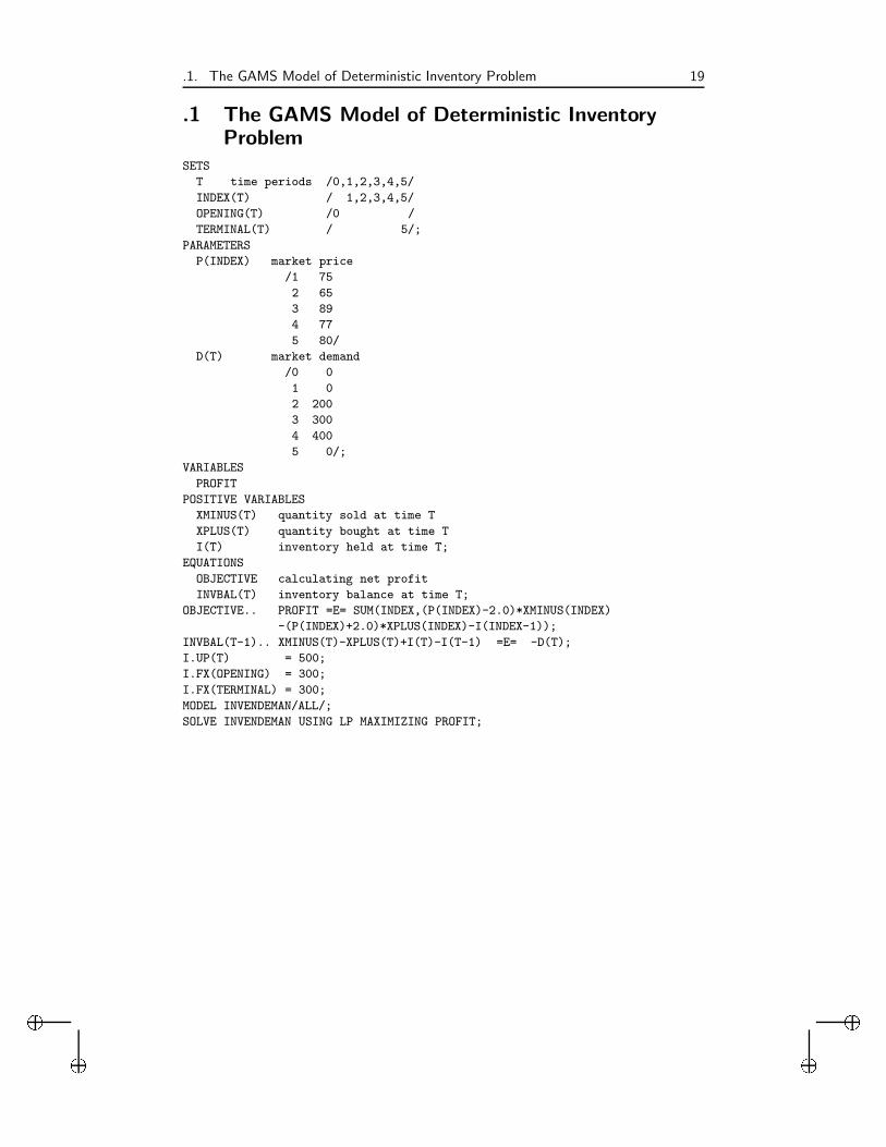
.1. The GAMS Model of Deterministic Inventory Problem 19

.1 The GAMS Model of Deterministic InventoryProblem

SETS

T time periods /0,1,2,3,4,5/

INDEX(T) / 1,2,3,4,5/

OPENING(T) /0 /

TERMINAL(T) / 5/;

PARAMETERS

P(INDEX) market price

/1 75

2 65

3 89

4 77

5 80/

D(T) market demand

/0 0

1 0

2 200

3 300

4 400

5 0/;

VARIABLES

PROFIT

POSITIVE VARIABLES

XMINUS(T) quantity sold at time T

XPLUS(T) quantity bought at time T

I(T) inventory held at time T;

EQUATIONS

OBJECTIVE calculating net profit

INVBAL(T) inventory balance at time T;

OBJECTIVE.. PROFIT =E= SUM(INDEX,(P(INDEX)-2.0)*XMINUS(INDEX)

-(P(INDEX)+2.0)*XPLUS(INDEX)-I(INDEX-1));

INVBAL(T-1).. XMINUS(T)-XPLUS(T)+I(T)-I(T-1) =E= -D(T);

I.UP(T) = 500;

I.FX(OPENING) = 300;

I.FX(TERMINAL) = 300;

MODEL INVENDEMAN/ALL/;

SOLVE INVENDEMAN USING LP MAXIMIZING PROFIT;

i

i

i

i

20 BIBLIOGRAPHY

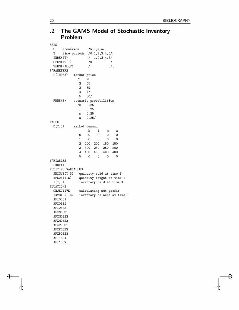
.2 The GAMS Model of Stochastic InventoryProblem

SETS

S scenarios /h,l,m,a/

T time periods /0,1,2,3,4,5/

INDEX(T) / 1,2,3,4,5/

OPENING(T) /0 /

TERMINAL(T) / 5/;

PARAMETERS

P(INDEX) market price

/1 75

2 65

3 89

4 77

5 80/

PROB(S) scenario probabilities

/h 0.25

l 0.25

m 0.25

a 0.25/

TABLE

D(T,S) market demand

h l m a

0 0 0 0 0

1 0 0 0 0

2 200 200 150 150

3 300 250 250 200

4 400 400 400 400

5 0 0 0 0

VARIABLES

PROFIT

POSITIVE VARIABLES

XMINUS(T,S) quantity sold at time T

XPLUS(T,S) quantity bought at time T

I(T,S) inventory held at time T;

EQUATIONS

OBJECTIVE calculating net profit

INVBAL(T,S) inventory balance at time T

AFI0SS1

AFI0SS2

AFI0SS3

AFXM0SS1

AFXM0SS2

AFXM0SS3

AFXP0SS1

AFXP0SS2

AFXP0SS3

AFI1SS1

AFI1SS2

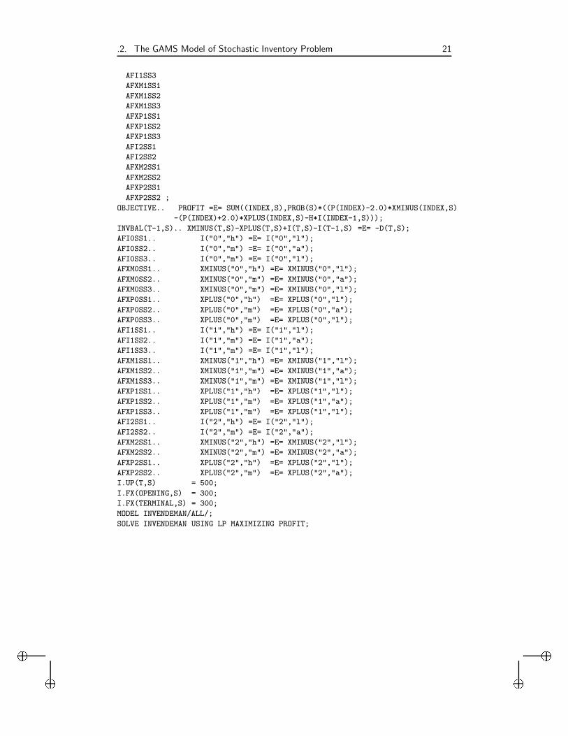
i

i

i

i

.2. The GAMS Model of Stochastic Inventory Problem 21

AFI1SS3

AFXM1SS1

AFXM1SS2

AFXM1SS3

AFXP1SS1

AFXP1SS2

AFXP1SS3

AFI2SS1

AFI2SS2

AFXM2SS1

AFXM2SS2

AFXP2SS1

AFXP2SS2 ;

OBJECTIVE.. PROFIT =E= SUM((INDEX,S),PROB(S)*((P(INDEX)-2.0)*XMINUS(INDEX,S)

-(P(INDEX)+2.0)*XPLUS(INDEX,S)-H*I(INDEX-1,S)));

INVBAL(T-1,S).. XMINUS(T,S)-XPLUS(T,S)+I(T,S)-I(T-1,S) =E= -D(T,S);

AFI0SS1.. I("0","h") =E= I("0","l");

AFI0SS2.. I("0","m") =E= I("0","a");

AFI0SS3.. I("0","m") =E= I("0","l");

AFXM0SS1.. XMINUS("0","h") =E= XMINUS("0","l");

AFXM0SS2.. XMINUS("0","m") =E= XMINUS("0","a");

AFXM0SS3.. XMINUS("0","m") =E= XMINUS("0","l");

AFXP0SS1.. XPLUS("0","h") =E= XPLUS("0","l");

AFXP0SS2.. XPLUS("0","m") =E= XPLUS("0","a");

AFXP0SS3.. XPLUS("0","m") =E= XPLUS("0","l");

AFI1SS1.. I("1","h") =E= I("1","l");

AFI1SS2.. I("1","m") =E= I("1","a");

AFI1SS3.. I("1","m") =E= I("1","l");



AFXM1SS3.. XMINUS("1","m") =E= XMINUS("1","l");



AFXP1SS3.. XPLUS("1","m") =E= XPLUS("1","l");

AFI2SS1.. I("2","h") =E= I("2","l");

AFI2SS2.. I("2","m") =E= I("2","a");





I.UP(T,S) = 500;

I.FX(OPENING,S) = 300;

I.FX(TERMINAL,S) = 300;

MODEL INVENDEMAN/ALL/;

SOLVE INVENDEMAN USING LP MAXIMIZING PROFIT;

Documents

Chapter 1 Stochastic Programming from Modeling Languagesgondzio/CV/spfml.pdf · 2002-05-17 · i i Chapter 1 Stochastic Programming from Modeling Languages Emmanuel Fragni ere1 and