Embed Size (px)
Citation preview

Chapter 1 Solutions
1.3 The probability density function for the gamma distribution is
f(t |α, λ) =λα
Γ(α)tα−1 exp(−λt).
What is the MTTF for the gamma distribution?
By definition,
MTTF =∫ ∞−∞
tf(t)dt
=∫ ∞
0
tλα
Γ(α)tα−1 exp(−λt)dt
=∫ ∞
0
λα
Γ(α)tα exp(−λt)dt
Recognizing that this is a Gamma(α+ 1, λ) distribution, we can write theintegral as ∫ ∞
0
λα
Γ(α)tα exp(−λt)dt =
λα
Γ(α)Γ(α+ 1)λα+1
=α
λ.
1.4 The probability density function for the Weibull distribution is
f(t |λ, β, θ) = λβ(t− θ)β−1 exp[−λ(t− θ)β
], 0 ≤ θ < t, λ > 0, β > 0.
What is the reliability function for the Weibull distribution?
By definition,
R(t) =∫ ∞t
f(s)ds
=∫ ∞t
λβ(s− θ)β−1 exp[−λ(s− θ)β ]ds.
Noticing that if u = − exp(−λ(s−θ)β), then du = λβ(s−θ)β−1 exp(−λ(s−θ)β)ds, we have
R(t) = − exp(−λ(s− θ)β) |∞t= exp(−λ(t− θ)β).
1.5 The probability density function for an exponential random variable is
f(t) = λe−λt, t > 0, λ > 0.
1

What is the average hazard rate for an exponential random variable?
In Example 1.1.3, it is shown that the cumulative hazard function is H(t) =λt. Therefore, by definition, AHR(t1, t2) = λt2−λt1
t2−t1 = λ(t2−t1)t2−t1 = λ.
1.7 Suppose that we are using the exponential distribution to model an item’slifetime.
(a) We observe that the item failed at 6 hours. What is the likelihoodfunction for this observation?
Let T ∼ Exponential(λ). Then f(t |λ) = λe−λt and the likelihoodfunction is l(λ | t = 6) = λe−6λ.
(b) We observe that the item failed at some time between 5 and 10 hours.What is the likelihood function for this observation?
From Table 1.6, we know that the likelihood function for an intervalcensored observation has the form F (tR) − F (tL). The cumulativedistribution function for an exponential random variable is F (t |λ) =1 − exp(−λt). Consequently, the likelihood function is l(λ | 5 ≤ t ≤10) = exp(−5λ)− exp(−10λ).
(c) We observe the item for 20 hours, and it does not fail. What is thelikelihood function for this observation?
From Table 1.6, we know that the likelihood function for a right-censored observation has the form 1 − F (tR). The cumulative dis-tribution function for an exponential random variable is F (t |λ) =1 − exp(−λt). Consequently, the likelihood function is l(λ | t ≥ 20) =1− exp(−20λ).
2

Chapter 2 Solutions
2.1 Suppose that we want to develop an informative prior distribution for theprobability of observing heads when we flip a coin. Suppose that we thinkthat the most likely probability of heads is 0.5 and that 0.75 would be“extreme.” Find the parameters of a beta density so that the median isapproximately 0.5 and the 0.9 quantile is 0.75.
The following R code can be used to solve this problem. q is a vector oflength 2 of quantiles, p is vector of length 2 of respective probabilities, initis a vector of length 2 of starting parameter values.
For this problem, α = β = 0.374.
parametersolver = function(qu,p,init) {qu <- qup <- p
betaoptim = function(param) {q1 <- qu[1]q2 <- qu[2]p1 <- p[1]p2 <- p[2](pbeta(q1,param[1],param[2])-p1)^2 + (pbeta(q2,param[1],param[2])-p2)^2
}
r = optim(init,betaoptim)
v = unlist(r)t = c(v[1],v[2])print(t)
}
parametersolver(c(.5,.9),c(.5,.75),c(1,1))
2.2 Suppose that we are going to flip a coin 20 times.
(a) Using a beta distribution, write down a prior density that describesyour uncertainty about the probability of “heads.”
Using the prior from problem 2.1, we might use a Beta(0.374, 0.374).This distribution has median is 0.50, the 0.025 quantile is .00022, andthe 0.975 quantile is 0.9998. This means there is 50% chance thatthe probability of heads is below 0.5, and it is very unlikely (a 5%chance) that the probability of getting heads will fall outside the in-
3

terval (0.00022, 0.99998). The pdf of this distribution is
p(π) =Γ(0.748)
Γ(0.374)Γ(0.374)π0.374−1(1− π)0.374−1 0 ≤ π ≤ 1
(b) Flip a coin 20 times and record the outcomes. Write down the likeli-hood function for the observed data.
Let Y = number of heads in 20 flips of a coin. Then Y ∼ Binomial(20,π). My 20 flips of penny had 11 heads, 9 tails. So the likelihood isgiven by
Lik(π) =(
2011
)π11(1− π)9
(c) Calculate the maximum likelihood estimate for the probability of “heads”and a 95% confidence interval.
log(Lik(π)) = l(π) = log
(2011
)+ 11log(π) + 9log(1− π)
l′(π) =
11π− 9
1− π= 0
⇒ π =1120
s.e.(π) =
√π(1− π)
n=
√.55(.45)
20= 0.111
A 95% confidence interval is given by π± z0.975s.e.(π) = (0.332, 0.768)
(d) Calculate the posterior distribution for the probability of “heads” anda 95% credible interval.
p(π | y = 11) ∝ π11(1− π)9π0.374−1(1− π)0.374−1
∝ Beta(11.374, 9.374)
Using R to find the 95% credible interval yields (0.337, 0.751).
qbeta(.025,11.374,9.374)qbeta(.975,11.374,9.374)
(e) Plot the log-likelihood function.
pi <- seq(0,1, by=.0001)l <- 11*log(pi) + 9*log(1-pi)plot(pi,l, type=’l’, main=’log-likelihood’, xlab=expression(pi),
ylab=expression(Log-lik(pi)))
4

0.0 0.2 0.4 0.6 0.8 1.0
-100
-80
-60
-40
-20
log-likelihood
π
log(Lik(π))
(f) Plot the prior density.
alpha <- .374beta <- .374beta <- (1/beta(alpha,beta)) * pi^(alpha-1) * (1-pi)^(beta-1)plot(pi, beta, type=’l’, main=’Prior Distribution’,
xlab=expression(pi), ylab=’beta(0.374, 0.374)’)
5

0.0 0.2 0.4 0.6 0.8 1.0
010
2030
4050
6070
Prior Distribution
π
beta
(0.3
74, 0
.374
)
(g) Plot the posterior density.
alpha <- 11.374beta <- 9.374beta <- (1/beta(alpha,beta)) * pi^(alpha-1) * (1-pi)^(beta-1)plot(pi, beta, type=’l’, main=’Posterior Distribution’,
xlab=expression(pi), ylab=’beta(11.374, 9.374)’)
6

0.0 0.2 0.4 0.6 0.8 1.0
01
23
Posterior Distribution
π
beta
(11.
374,
9.3
74)
(h) Calculate the Bayes’ factor comparing a uniform prior density to yourinformative prior density.
Let M1 be the model with a uniform prior and M2 be the model witha Beta(0.374, 0.374) prior. Then
m1(11 |M1) =∫ 1
0
(2011
)π11(1− π)9dπ
=(
2011
)Γ(12)Γ(10)
Γ(22)
∫ 1
0
Γ(22)Γ(12)Γ(10)
π12−1(1− π)10−1dπ
= 1/21= 0.04761905
m2(11 |M2) =∫ 1
0
(2011
)π11(1− π)9π0.374−1(1− π)0.374−1dπ
=(
2011
)Γ(11.374)Γ(9.374)
Γ(20.748)= 0.1175762
So the Bayes’ factor in favor of M1 is 0.047619050.1175762 = 0.405.
2.3 Consider again the fluid breakdown times introduced in Sect. 2.5. Twomodels were proposed for these data. The first incorporated a normal likeli-hood function and a noninformative prior distribution; the second a normal
7

likelihood function and a conjugate inverse-gamma/normal prior distribu-tion. Now suppose that the properties of the manufacturing process werecontrolled when these samples of lubricant were produced so that it is knownthat the true mean of the sample values must lie between 6.0 and 7.4 (on theoriginal measurement scale). No further information is available concerningthe value of the variance parameter σ2.
(a) Assume that the joint prior distribution for (µ, σ2) is proportional to1/σ2 whenever µ ∈ (log(6.0), log(7.4)), and is 0 otherwise. Find anexpression for a function that is proportional to the joint posterior dis-tribution.
p(µ, σ2 |y) ∝ (σ2)−n2−1exp
[− 1
2σ2
n∑i=1
(yi − µ)2
]I[µ ∈ (log(6.0), log(7.4))]
(b) Find a function that is proportional to the marginal posterior distri-bution of µ.
p(µ |y) ∝[1 +
(µ− y)2
(n− 1)s2/n
]−n/2I[µ ∈ (log(6.0), log(7.4)]
(c) Find a function that is proportional to the marginal posterior distri-bution of σ2.
p(σ2 |y) ∝∫ log(7.4)
log(6.0)
(σ2)−n/2−1exp
[− 1
2σ2
n∑i=1
(yi − µ)2
]dµ
2.4 Show that the beta distribution is the conjugate prior distribution for thebinomial likelihood.
Suppose that we have data X ∼ Binomial(n, π), and that the prior dis-tribution for π is Beta(α, β). Then the posterior distribution of π is givenas
p(π |x, α, β) ∝ πx(1− π)n−xπα−1(1− π)β−1
∝ πx+α−1(1− π)n−x+β−1,
which is Beta(x+ α, n− x+ β).
2.5 Show that the gamma distribution is the conjugate prior distribution forthe mean of a Poisson likelihood.
8

Suppose that we have data Xi ∼ Poisson(λ), and that the prior distributionfor λ is Gamma(α, β). Then the posterior distribution of π is given as
p(λ | ~x, α, β) ∝ λPni=1 xi exp(−nλ)λα−1 exp(−βλ)
∝ λα+Pni=1 xi−1 exp(−(β + n)λ),
which is Gamma(α+∑ni=1 xi, n+ β).
2.6 Show that the gamma distribution is the conjugate prior distribution forthe exponential likelihood.
Suppose that we have data Xi ∼ Exponential(λ), and that the prior distri-bution for λ is Gamma(α, β). Then the posterior distribution of π is givenas
p(λ | ~x, α, β) ∝ λn exp(−λn∑i=1
xi)λα−1 exp(−βλ)
∝ λn+α−1 exp(−(β +n∑i=1
xi)λ),
which is Gamma(α+ n, β +∑ni=1 xi).
2.7 Derive the mean and variance for the lognormal distribution.
E[X] =∫ ∞
0
x1
x√
2πσ2exp
[− 1
2σ2(log(x)− µ)2
]dx
=∫ ∞−∞
1√2πσ2
exp(− 12σ2
y2) exp(y + µ)dy
=∫ ∞−∞
1√2πσ2
exp(− 12σ2
(y − σ2)2) exp(µ+σ2
2)dy
= exp(µ+σ2
2).
E[X2] =∫ ∞
0
x2 1x√
2πσ2exp
[− 1
2σ2(log(x)− µ)2
]dx
=∫ ∞−∞
1√2πσ2
exp(− 12σ2
y2) exp(2y + 2µ)dy
=∫ ∞−∞
1√2πσ2
exp(− 12σ2
(y − 2σ2)2) exp(2µ+ 2σ2)dy
= exp(2µ+ 2σ2).
9
The mean of the lognormal distribution is E[X] = exp(µ + σ2
2 ), and thevariance is V ar[X] = E[X2]− (E[X]2) = exp(2µ+ 2σ2)− exp(2µ+ σ2).
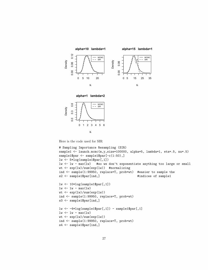
2.8 Suppose we are using an Exponential(λ) distribution to model the lifetimesof n items.
(a) Find the maximum likelihood estimator of λ.
The log-likelihood function for λ is log(L(λ |~t)) = n log(λ)−λ∑ni=1 ti.
Taking derivatives,
d
dλlog(L(λ |~t)) =
n
λ−
n∑i=1
ti.
Setting the derivative equal to zero and solving for λ gives nλ =
∑ni=1 ti,
or λ = nPni=1 ti
.
(b) Assume n is large and find the standard error of λ.
The second derivative of the log-likelihood is
d2
dλ2log(L(λ |~t)) = − n
λ2.
The observed Fisher information is λ√n
=√nPn
i=1 ti.
(c) Suppose that we observed n = 50 items and that∑50i=1 ti = 25. Find
a 90% confidence interval for λ.
A 90% confidence interval for λ is
(λ− 1.645se(λ), λ+ 1.645se(λ)),
which is (50/25 − 1.645√
(50)/25, 50/25 + 1.645√
(50)/25) = (2 −0.465, 2 + 0.465) = (1.535, 2.464).
(d) Suppose that λ ∼ Gamma(1, 2). Find the posterior distribution for λ.
From Exercise 2.6, the posterior distribution is Gamma(α + n, β +∑ni=1 xi) = Gamma(1 + 50, 2 + 25) = Gamma(51, 27).
(e) Suppose that we observed n = 50 items and that∑50i=1 ti = 25. What
is the posterior probability that λ falls in the 90% confidence intervalfound in (c)?
10

∫ 2.464
1.535
2751
Γ(51)exp(−27x)x50dx = 0.979.
11

Chapter 3
3.1 Suppose that X ∼ Normal(0, 1) and Y = exp(X).
(a) Use the change of variables technique to calculate the probability den-sity function, mean, and variance of Y .
X ∼ Normal(0,1) f(x) = 1√2πe−x
2/2
Y ∼ eX g−1(y) = log(y) ddy g−1(y) = 1/y
fY (y) = fX(g−1(y))∣∣∣∣ ddy g−1(y)
∣∣∣∣=
1√2πy
exp[−1
2(log(y))2
], y > 0
So Y ∼ LogNormal(0, 1) with E(Y) = e1/2 = 1.648 and Var(Y) =e2 − e = 4.671
(b) Draw a random sample X1, . . . , X10,000 from a Normal(0, 1) distribu-tion. Set Yi = exp(Xi). Draw a histogram of the Yi and overlay a plotof the probability density function of Y .
x <- rnorm(10000,0,1)y <- exp(x)f <- function(x){f <- 1/(x*sqrt(2*pi))*exp(-.5*(log(x))^2)}hist(y, freq=F, main=’Histogram of 10,000 random draws from Y
with pdf f(y)’)curve(f, col=2, add=T)
12

Histogram of 10,000 random draws from Y with pdf f(y)
y
Density
0 10 20 30 40 50
0.00
0.05
0.10
0.15
(c) Estimate the probability density function, mean, and variance of Yusing the random sample.
quantile(y,c(.025,.05,.5,.95,.975))mean(y)var(y)
QuantilesParameter Mean Variance 0.025 0.050 0.500 0.950 0.975
λ 1.66 4.64 0.14 0.19 0.99 5.17 7.04
3.2 Suppose we perform an experiment where the data have a Poisson(λ) sam-pling density. We describe our uncertainty about λ using a Gamma priordensity with parameters α and β. We also describe our uncertainty aboutα and β using independent Gamma prior densities.
(a) Simulate 50 observations from a Poisson distribution with parameterλ = 5.
x <- rpois(50,5)
(b) Choose diffuse prior densities for α and β.Let α ∼ Gamma(0.001, 0.001) and β ∼ Gamma(0.001, 0.001).
13

(c) Implement an MCMC algorithm to calculate posterior densities for λ,α, and β.
Evaluating the posterior distribution on the log scale helps to min-imize numerical issues, as does transforming the parameters to realline. logpost() is a function that computes the log of the posterior.logpost2() is a function that computes the log transformed parame-ters.
library(coda)library(MASS)library(LearnBayes)library(MCMCpack)
logpost <- function(theta, data){alpha = theta[1]beta = theta[2]lambda = theta[3]n = length(data)sumd = sum(data)val = (sumd + alpha -1)*log(lambda) - lambda*(n+beta)
+ alpha*log(beta) - lgamma(alpha) + (.001-1)*log(alpha*beta)- .001*(alpha+beta)
return(val)}
logpost2 <- function(theta, data){ #theta is the log of above thetaa = theta[1]b = theta[2]l = theta[3]return(logpost(c(exp(a), exp(b), exp(l)), data) + a + b + l)#remember the Jacobian!}
mu.x <- mean(x)theta <- c(1,1,mu.x); theta <- log(theta)fit <- laplace(logpost2, theta, x)
sample <- gibbs(logpost2, fit$mode, 10000, c(.13,.13,.13), data=x)sample$acceptplot(as.mcmc(sample$par))plot(sample$par[,1], sample$par[,2], xlab=expression(alpha),
ylab=expression(beta), main=’alpha vs beta from Gibbs sampler’)
sample2 <- rwmetrop(logpost2, list(var=fit$var, scale=2), fit$mode,10000, x)
14

sample2$acceptplot(as.mcmc(sample2$par))plot(sample2$par[,1], sample2$par[,2])
gibbs() and rwmetrop() are part of the LearnBayes package andas.mcmc() is in the MCMCpack package. rwmetrop is a random walkMetropolis algorithm, and gibbs is a Metropolis-within-Gibbs algo-rithm. If you would like addition reading and examples with thesefunctions I recommend Jim Albert’s Bayesian Computation with R(Springer).
The Gibbs sampler has problems mixing, probably due to the highcorrelation between α and β.
0 2000 4000 6000 8000 10000
13
5
Iterations
Trace of var1
0 1 2 3 4 5 6 7
0.00.20.4
N = 10000 Bandwidth = 0.2012
Density of var1
0 2000 4000 6000 8000 10000
-11
3
Iterations
Trace of var2
-2 -1 0 1 2 3 4 5
0.00.20.4
N = 10000 Bandwidth = 0.1989
Density of var2
0 2000 4000 6000 8000 10000
1.5
1.8
Iterations
Trace of var3
1.4 1.5 1.6 1.7 1.8 1.9
0246
N = 10000 Bandwidth = 0.01083
Density of var3
15

2 3 4 5 6
01
23
4
alpha vs beta from Gibbs sampler
log(α)
log(β)
By sampling α and β together, the Metropolis algorithm mixes betterthan the Gibbs in this problem.
0 2000 4000 6000 8000 10000
-50
5
Iterations
Trace of var1
-5 0 5 10
0.00
0.10
N = 10000 Bandwidth = 0.4063
Density of var1
0 2000 4000 6000 8000 10000
-10
05
Iterations
Trace of var2
-10 -5 0 5
0.00
0.10
N = 10000 Bandwidth = 0.4035
Density of var2
0 2000 4000 6000 8000 10000
1.31.51.7
Iterations
Trace of var3
1.3 1.4 1.5 1.6 1.7
02
46
N = 10000 Bandwidth = 0.01122
Density of var3
(d) Is λ = 5 contained in a 90% posterior credible interval for λ?
quantile(exp(sample2$par[,3]), c(.05,.95))
16

Yes. Remember that the above graphs are based on the log of theparameters. A 90% posterior credible interval for λ is (4.06, 5.05).
3.3 Consider again the fluid breakdown times introduced in Sect. 2.5. Twomodels were proposed for these data. The first incorporated a normal like-lihood function and a noninformative prior density; the second, a normallikelihood function and a conjugate inverse-gamma/normal prior density.Now suppose that the properties of the manufacturing process were con-trolled when these samples of lubricant were produced so that it is knownthat the true mean of the sample values must lie between 6.0 and 7.4 (on theoriginal measurement scale). No further information is available concerningthe value of the variance parameter σ2. Assume that the joint prior densityfor (µ, σ2) is proportional to 1/σ2 whenever µ ∈ (log(6.0), log(7.4)), and is0 otherwise.
(a) Find an expression for a function that is proportional to the joint pos-terior density.
We can write the joint prior of µ and σ2 with the use of an indicatorfunction. i.e., p(µ, σ2) ∝ 1
σ2 I[log(6.0) < µ < log(7.4)]. Then
p(µ, σ2 |y) ∝ (σ2)−n2−1exp
[− 1
2σ2
n∑i=1
(yi − µ)2
]I[log(6.0) < µ < log(7.4)].
(b) Describe a hybrid Gibbs/Metropolis-Hastings algorithm for samplingfrom the joint posterior density.
Z ∼ Normal(0, 1) and c1 and c2 are specified constants for µ and σrespectively.0. Initialize j = 0, and starting vales µ(j), σ2(j).
1. Generate µ∗ from µ(j) + c1Z.
2. Compute r =(σ2(j))−
n2 −1exp
h− 1
2σ2(j)
Pni=1(yi−µ∗)2
iI[log(6.0)<µ∗<log(7.4)]
(σ2(j))−n2 −1exp
h− 1
2σ2(j)
Pni=1(yi−µ(j))2
iI[log(6.0)<µ(j)<log(7.4)]
.
3. Draw u from a Uniform(0, 1) distribution.
4. If u ≤ r, set µ(j+1) = µ∗. Otherwise, set µ(j+1) = µ(j).
5. Generate σ2∗ from σ2(j) + c2Z.
6. Compute r =(σ2∗)−
n2 −1exp[− 1
2σ2∗Pni=1(yi−µ(j))2]I[log(6.0)<µ(j)<log(7.4)]
(σ2(j))−n2 −1exp
h− 1
2σ2(j)
Pni=1(yi−µ(j))2
iI[log(6.0)<µ(j)<log(7.4)]
.
7. Draw u from a Uniform(0, 1) distribution.
17

8. If u ≤ r, set σ2(j+1) = σ2∗. Otherwise, set σ2(j+1) = σ2(j).
9. Increment j and return to 1.
3.4 Implement the algorithm in Fig. 3.1. Use batch means to compute thesimulation error.
m = 10000pi = array(0, dim=c(m,1))pi0 = 0.5pi1 = pi0for (j in 1:m){pi.star = runif(1,.1,.9)r = (pi.star^3* (1-pi.star)^8)/(pi1^3*(1-pi1)^8)u = runif(1) <= rpi1 = pi.star*(u==1) + pi1*(u==0)pi[j] = pi1}
To calculate the simulation error via batch means:
# 1. Get the means of the batchesb <- 80v <- m/b; v #make sure v is a whole numbermeans <- array(0, dim=c(b,1))for(i in 1:b){
means[i,1] = mean(pi[(v*i - (v-1)):(v*i)])}
# 2. Check that lag 1 autocorrelation of batch means is less than 0.1library(coda)autocorr(as.mcmc(means), 1)
# 3. Compute an estimate of the simulation errormu <- mean(means)stderror <- sd(means)/sqrt(b)
The simulation standard error is 0.0019. You can also get this using summary(as.mcmc(pi))from the coda package.
3.5 Implement the algorithm in Fig. 3.4. Calculate the autocorrelation for thechain.
data <- read.table(’http://www.bayesianreliability.com/wp-content/uploads/2009/06/table23.txt’, header=T)
18

y <- log(data[,1])n = length(y)m = 5000par = array(0, dim=c(m,2))par1 = c(0,0.5)s1 = 0.5; s2 = 1for(j in 1:m){
mu.star = rnorm(n=1, mean=par1[1], sd=s1)r = exp(-sum((y-mu.star)^2)/(2*par1[2]))/
exp(-sum((y-par1[1])^2)/(2*par1[2]))u = runif(1) <= rpar1[1] = mu.star*(u==1) + par1[1]*(u==0)nu = rnorm(1,0,sd=s2)var.star = par1[2]*exp(nu)r = (var.star^(-n/2)*exp(-sum((y-par1[1])^2)/(2*var.star)))/
(par1[2]^(-n/2)*exp(-sum((y-par1[1])^2)/(2*par1[2])))u = runif(1) <= rpar1[2] = var.star*(u==1) + par1[2]*(u==0)par[j,] = par1
}
# Calculate the autocorrelationautocorrelation <- function(par, lag){
l = lagA = par[1:(m-l),]B = par[(1+l):m,]mu1 = mean(par[,1])mu2 = mean(par[,2])cor1 = (sum((A[,1]-mu1)*(B[,1]-mu1))/(m-l))/
(sum((par[,1]-mu1)^2)/m)cor2 = (sum((A[,2]-mu2)*(B[,2]-mu2))/(m-l))/
(sum((par[,2]-mu2)^2)/m)return(c(cor1, cor2))
}autocorrelation(par, 1)
The autocorrelation for the chain (i.e. lag 1) is 0.8565168 and 0.7419024for µ and σ2. You can also get this using autocorr.diag(as.mcmc(par))from the coda package.
3.6 In the analysis of the launch vehicle success probabilities described in Ex-ample 3.4, the hyperparameters α and λ were assigned values of 5 and 1,respectively.
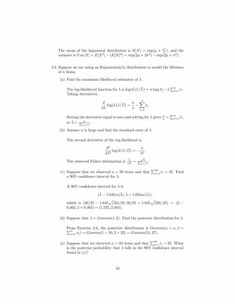
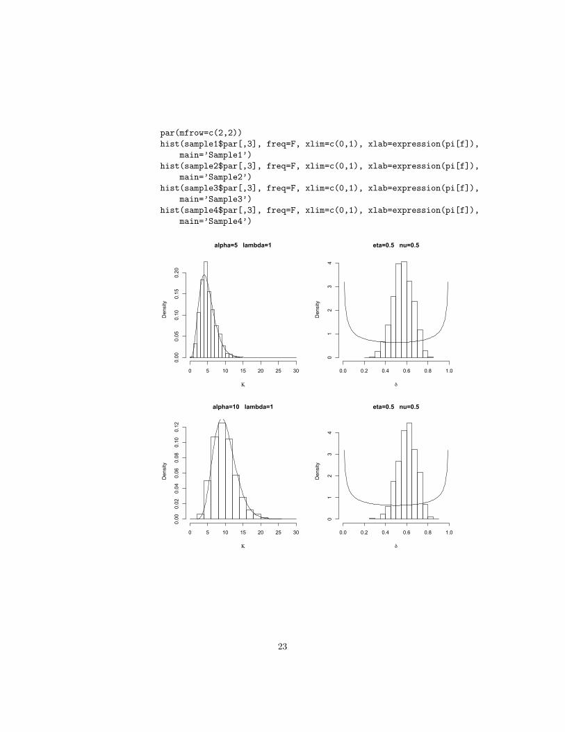
(a) Perform a sensitivity analysis for α and λ by varying their values overa suitable range.
19

data <- read.table(’http://www.bayesianreliability.com/wp-content/uploads/2009/06/table31.txt’, header=T)
m <- data[,3]y <- data[,2]launch.mcmc <- function(m, y, size, alpha, lambda, eta, nu){
K1 = alpha/lambdaD1 = eta/(eta+nu)n = length(m)par1 = array(0, dim=c(size,2))par2 = array(0, dim=c(n,1))arateK = 0; arateD = 0# We use the log of the posterior for a more stable algorithmlogpost = function(K,D){
val=0for(i in 1:n){
val = val + (y[i]+K*D-1)*log(par2[i]) +(m[i]-y[i]+K-K*D-1)*log(1-par2[i])}
val = val + n*lgamma(K) - n*lgamma(K*D) - n*lgamma(K-K*D) +(alpha-1)*log(K) - lambda*K + (eta-1)*log(D) + (nu-1)*log(1-D)
return(val)}for (j in 1:size){
for (i in 1:n){a = y[i] + K1*D1b = m[i] - y[i] + K1 - K1*D1par2[i] = rbeta(1,a,b)
}z = rnorm(1)K.star = K1*exp(z)# use log(r) because we want to use the log of the posteriorlogr = logpost(K.star,D1) + log(K.star) - (logpost(K1,D1) + log(K1))u = runif(1) <= exp(logr)arateK = arateK + uK1 = K.star*(u==1) + K1*(u==0)c = mean(par2)D.star = rbeta(1, K1*c, K1*(1-c))logr = (logpost(K1,D.star) + (K1*c-1)*log(D1/D.star)) -
(logpost(K1,D1) + (K1*(1-c)-1)*log((1-D.star)/(1-D1)))u = runif(1) <= exp(logr)arateD = arateD + uD1 = D.star*(u==1) + D1*(u==0)par1[j,] = c(K1,D1)
}arate = c(arateK, arateD); arate = array(arate/size, dim=c(1,2))
20

colnames(arate) = c("Kappa", "Delta")pif <- array(0, dim=c(size,1))for(i in 1:size){
Kj = par1[i,1]Dj = par1[i,2]pif[i] = rbeta(1, Kj*Dj, Kj*(1-Dj))
}par = cbind(par1, pif)colnames(par) = c("Kappa", "Delta", "Pif")ans = list(par = par, accept = arate)return(ans)}
sample1 <- launch.mcmc(m,y,size=10000, alpha=5, lambda=1, eta=.5, nu=.5)sample1$par <- sample1$par[-c(1:50),]mu <- array(apply(sample1$par, 2, mean), dim=c(3,1))st.dev <- array(apply(sample1$par, 2, sd), dim=c(3,1))quant <- rbind(quantile(sample1$par[,1], c(.025,.05,.5,.95,.975)),
quantile(sample1$par[,2], c(.025, .05, .5, .95, .975)),quantile(sample1$par[,3], c(.025, .05, .5, .95, .975)))
summary = array(c(mu, st.dev, quant), dim=c(3,7))colnames(summary) = c("Mean", "Std Dev", "2.5%", "5%", "50%",
"95%", "97.5%")rownames(summary) = c("Kappa", "Delta", "Pif")summarypar(mfrow=c(1,2))hist(sample1$par[,1], freq=F, xlim=c(0,30), xlab=expression(Kappa),
main=’alpha=5 lambda=1’)curve(dgamma(x, shape=5, scale=1), add=T)hist(sample1$par[,2], xlab=expression(delta), xlim=c(0,1), freq=F,
main=’eta=0.5 nu=0.5’)curve(dbeta(x, .5,.5), add=T)
sample2 <- launch.mcmc(m,y,size=5000, alpha=10, lambda=1, eta=.5, nu=.5)sample2$par <- sample2$par[-c(1:50),]mu <- array(apply(sample2$par, 2, mean), dim=c(3,1))st.dev <- array(apply(sample2$par, 2, sd), dim=c(3,1))quant <- rbind(quantile(sample2$par[,1], c(.025,.05,.5,.95,.975)),
quantile(sample2$par[,2], c(.025, .05, .5, .95, .975)),quantile(sample2$par[,3], c(.025, .05, .5, .95, .975)))
summary = array(c(mu, st.dev, quant), dim=c(3,7))colnames(summary) = c("Mean", "Std Dev", "2.5%", "5%", "50%",
"95%", "97.5%")rownames(summary) = c("Kappa", "Delta", "Pif")summarypar(mfrow=c(1,2))
21

hist(sample2$par[,1], freq=F, xlim = c(0,30), xlab=expression(Kappa),main=’alpha=10 lambda=1’)
curve(dgamma(x, shape=10, scale=1), add=T)hist(sample2$par[,2], xlab=expression(delta), xlim=c(0,1), freq=F,
main=’eta=0.5 nu=0.5’)curve(dbeta(x, .5,.5), add=T)
sample3 <- launch.mcmc(m,y,size=5000, alpha=15, lambda=1, eta=.5, nu=.5)sample3$par <- sample3$par[-c(1:50),]mu <- array(apply(sample3$par, 2, mean), dim=c(3,1))st.dev <- array(apply(sample3$par, 2, sd), dim=c(3,1))quant <- rbind(quantile(sample3$par[,1], c(.025,.05,.5,.95,.975)),
quantile(sample3$par[,2], c(.025, .05, .5, .95, .975)),quantile(sample3$par[,3], c(.025, .05, .5, .95, .975)))
summary = array(c(mu, st.dev, quant), dim=c(3,7))colnames(summary) = c("Mean", "Std Dev", "2.5%", "5%", "50%",
"95%", "97.5%")rownames(summary) = c("Kappa", "Delta", "Pif")summarypar(mfrow=c(1,2))hist(sample3$par[,1], freq=F, xlim = c(0,30), xlab=expression(Kappa),
main=’alpha=15 lambda=1’)curve(dgamma(x, shape=15, scale=1), add=T)hist(sample3$par[,2], xlab=expression(delta), xlim=c(0,1), freq=F,
main=’eta=0.5 nu=0.5’)curve(dbeta(x, .5,.5), add=T)
sample4 <- launch.mcmc(m,y,size=5000, alpha=1, lambda=2, eta=.5, nu=.5)sample4$par <- sample4$par[-c(1:50),]mu <- array(apply(sample4$par, 2, mean), dim=c(3,1))st.dev <- array(apply(sample4$par, 2, sd), dim=c(3,1))quant <- rbind(quantile(sample4$par[,1], c(.025,.05,.5,.95,.975)),
quantile(sample4$par[,2], c(.025, .05, .5, .95, .975)),quantile(sample4$par[,3], c(.025, .05, .5, .95, .975)))
summary = array(c(mu, st.dev, quant), dim=c(3,7))colnames(summary) = c("Mean", "Std Dev", "2.5%", "5%", "50%",
"95%", "97.5%")rownames(summary) = c("Kappa", "Delta", "Pif")summarypar(mfrow=c(1,2))hist(sample4$par[,1], freq=F, xlim = c(0,30), xlab=expression(Kappa),
main=’alpha=1 lambda=2’)curve(dgamma(x, shape=1, scale=2), add=T)hist(sample4$par[,2], xlab=expression(delta), xlim=c(0,1), freq=F,
main=’eta=0.5 nu=0.5’)curve(dbeta(x, .5,.5), add=T)
22
par(mfrow=c(2,2))hist(sample1$par[,3], freq=F, xlim=c(0,1), xlab=expression(pi[f]),
main=’Sample1’)hist(sample2$par[,3], freq=F, xlim=c(0,1), xlab=expression(pi[f]),
main=’Sample2’)hist(sample3$par[,3], freq=F, xlim=c(0,1), xlab=expression(pi[f]),
main=’Sample3’)hist(sample4$par[,3], freq=F, xlim=c(0,1), xlab=expression(pi[f]),
main=’Sample4’)
alpha=5 lambda=1
Κ
Density
0 5 10 15 20 25 30
0.00
0.05
0.10
0.15
0.20
eta=0.5 nu=0.5
δ
Density
0.0 0.2 0.4 0.6 0.8 1.0
01
23
4
alpha=10 lambda=1
Κ
Density
0 5 10 15 20 25 30
0.00
0.02
0.04
0.06
0.08
0.10
0.12
eta=0.5 nu=0.5
δ
Density
0.0 0.2 0.4 0.6 0.8 1.0
01
23
4
23

alpha=15 lambda=1
Κ
Density
0 5 10 15 20 25 30
0.00
0.02
0.04
0.06
0.08
0.10
0.12
eta=0.5 nu=0.5
δ
Density
0.0 0.2 0.4 0.6 0.8 1.0
01
23
45
alpha=1 lambda=2
Κ
Density
0 5 10 15 20 25 30
0.0
0.1
0.2
0.3
0.4
0.5
0.6
0.7
eta=0.5 nu=0.5
δ
Density
0.0 0.2 0.4 0.6 0.8 1.0
01
23
4
24

Sample1
πf
Density
0.0 0.2 0.4 0.6 0.8 1.0
0.0
1.0
Sample2
πf
Density
0.0 0.2 0.4 0.6 0.8 1.0
0.0
1.0
2.0
Sample3
πf
Density
0.0 0.2 0.4 0.6 0.8 1.0
0.0
1.0
2.0
Sample4
πf
Density
0.0 0.2 0.4 0.6 0.8 1.0
0.0
1.0
2.0
QuantilesParameter Mean Std Dev 0.05 0.95
sample1 κ = 5 5.12 2.12 2.25 9.04δ = 0.5 0.56 0.09 0.40 0.71
πf 0.56 0.23 0.16 0.91sample2 κ = 10 9.73 3.21 5.26 15.54
δ = 0.5 0.60 0.09 0.46 0.74πf 0.60 0.18 0.28 0.87
sample3 κ = 15 14.62 3.49 9.40 20.82δ = 0.5 0.62 0.08 0.48 0.74
πf 0.62 0.15 0.36 0.85sample4 κ = 0.5 1.32 0.64 0.53 2.49
δ = 0.5 0.46 0.12 0.27 0.66πf 0.46 0.35 0.00 0.99
An alternative to running an MCMC algorithm several times, as doneabove, is to do sampling importance resampling (SIR). For more infor-mation see Albert’s Bayesian Computation with R section 5.10 (Springer).The idea is that we can take a weighted bootstrap sample (with replace-ment) from the current posterior distribution to get a sample from thenew posterior distribution. The weights are computed by calculatingNewPosteriorOldPosterior . Then convert the weights to probabilities by normalizing
them to add to 1. Lastly, resample the sample from the OLD posteriorusing these probabilities to get a sample the NEW posterior.
25

In this exercise, we are on the log scale. Since we are only interestedin how changes to the prior on K affects the posterior distribution,
log(NewPosterior
OldPosterior
)= log
(p(K |α, λ)NEWp(K |α, λ)OLD
).
Then the weights to get an approximation to sample2 above are
log(p(K |α, λ)NEWp(K |α, λ)OLD
)∝ log
(K9e−K
K4e−K
)= 5 logK.
For this particular example, SIR works well for getting an approxima-tion to sample2 and sample4 above. However, for sample3, SIR givesa poor approximation. The graph below shows the marginal posteriorthat we will be sampling from, along with the three new priors on Kthat we used for samples 2 through 4 above. With SIR, be careful thatyou have enough points in the tails that will be heavily weighted inthe resampling. To get a decent approximation to sample2 I had toincrease my MCMC sample size to 100,000 in order to get sufficientdata in the upper tail. We can also see that for sample3, our samplesfor the marginal posterior do not extend nearly far enough to get agood approximation for that distribution.
0 5 10 15 20 25 30
0.0
0.1
0.2
0.3
0.4
0.5
!
Density
Marginal Post of K
Gamma(10,1)
Gamma(15,1)
Gamma(1,2)
The graphs below show how the three SIR approximations (resam-pled from the 100,000 size MCMC) compared to the three additionalMCMC runs called sample2, sample3 and sample4 above.
26
0 5 10 20
0.00
0.06
0.12
alpha=10 lambda=1
Κ
Density
MCMCSIR
0 5 15 25 35
0.00
0.06
alpha=15 lambda=1
Κ
Density
MCMCSIR
0 1 2 3 4 5 6
0.0
0.3
0.6
alpha=1 lambda=2
Κ
Density
MCMCSIR
Here is the code used for SIR
# Sampling Importance Resampling (SIR)sample1 <- launch.mcmc(m,y,size=100000, alpha=5, lambda=1, eta=.5, nu=.5)sample1$par <- sample1$par[-c(1:50),]lw <- 5*log(sample1$par[,1])lw <- lw - max(lw) #so we don’t exponentiate anything too large or smallwt <- exp(lw)/sum(exp(lw)) #normalizingind <- sample(1:99950, replace=T, prob=wt) #easier to sample thes2 <- sample1$par[ind,] #indices of sample1
lw <- 10*log(sample1$par[,1])lw <- lw - max(lw)wt <- exp(lw)/sum(exp(lw))ind <- sample(1:99950, replace=T, prob=wt)s3 <- sample1$par[ind,]
lw <- -4*log(sample1$par[,1]) - sample1$par[,1]lw <- lw - max(lw)wt <- exp(lw)/sum(exp(lw))ind <- sample(1:99950, replace=T, prob=wt)s4 <- sample1$par[ind,]
27

(b) Report how changes in the values assumed for λ and α impact theposterior means of other model parameters.
The choice of K has a small effect on the marginal posterior distri-bution of δ. As we increase K, the mean of the marginal posterior ofδ increases slightly. The posterior predictive mean for πf is roughlyequal to the posterior mean of δ, so our choice of K has the same effecton the posterior mean of πf as that of δ.
3.7 Derive the conditional densities described in Example 3.4 for the randomeffects model.
The joint posterior distribution is
p(µ, σ2, κ, β |y) ∝ κ−9.5(σ2)−31exp
−0.25κ− 1
2σ2κ
10∑j=1
β2j −
12σ2
5∑i=1
10∑j=1
(yij − βj − µ)2
.So the full conditional densities are
p(µ |β, σ2, κ,y) ∝ exp
− 12σ2
5∑i=1
10∑j=1
(yij − βj − µ)2
∝ exp
− 12σ2
5∑i=1
10∑j=1
(µ− (yij − βj))2
∝ exp
− 12σ2
50µ2 − 2µ5∑i=1
10∑j=1
(yij − βj)
∝ exp
− 12(σ2/50)
µ− 150
5∑i=1
10∑j=1
(yij − βj)
2
∝ 1√2π(σ2/50)
exp
− 12(σ2/50)
µ− 150
5∑i=1
10∑j=1
(yij − βj)
2
∼ Normal
150
5∑i=1
10∑j=1
(yij − βj),σ2
50
28

p(βj |βi6=j, µ, σ2, κ,y) ∝ exp
− 12σ2κ
10∑j=1
β2j −
12σ2
5∑i=1
(yij − βj − µ)2
∝ exp
[− 1
2σ2
(1κβ2j +
5∑i=1
(βj − (yij − µ))2
)]
∝ exp
[− 1
2σ2
(1κβ2j + 5β2
j − 2βj5∑i=1
(yij − µ) +5∑i=1
(yij − µ)2
)]
∝ exp
−5 + 1/κ2σ2
(βj −
∑5i=1(yij − µ)5 + 1/κ
)2
∝ 1√2π( 1
5/σ2+1/(κσ2) )exp
− 5σ2 + 1
κσ2
2σ2
(βj −
∑5i=1(yij − µ)/σ2
5σ2 + 1
κσ2
)2
∼ Normal
(∑5i=1(yij − µ)/σ2
5/σ2 + 1/(κσ2),
15/σ2 + 1/(κσ2)
)
p(σ2 | β, µ, κ,y)
∝ (σ2)−31exp
− 12σ2κ
10∑j=1
β2j −
12σ2
5∑i=1
10∑j=1
(yij − βj − µ)2
∝
[12
∑5i=1
∑10j=1(yij − βj − µ)2 + 1
2σ2
∑10j=1
β2j
κ
]30
Γ(30)(σ2)−(30+1)
×exp
− 1σ2
12
5∑i=1
10∑j=1
(yij − βj − µ)2 +12
10∑j=1
β2j
κ
∼ InverseGamma
30,12
5∑i=1
10∑j=1
(yij − βj − µ)2 +12
10∑j=1
β2j
κ
29

p(κ |β, µ, σ2,y) ∝ κ−(8.5+1)exp
−0.25κ− 0.5σ2κ
10∑j=1
β2j
∝ κ−(8.5+1)exp
− 1κ
0.25 + 0.510∑j=1
β2j /σ
2
∼ InverseGamma
8.5, 0.25 + 0.510∑j=1
β2j /σ
2
30

Chapter 4
4.1 The Beta(293, 0.5) prior for π yields a posterior with a median of 0.999and a 95% credible interval of (0.990, 1.000), whose length is 0.010. Theuniform prior (i.e., Beta(1, 1)) yields a posterior with a median of 0.997and a 95% credible interval of (0.983, 1.000), whose length is 0.017.
4.3 The likelihood is∏ni=1(λti)yi exp(−λti)/yi! ∝ λ
Pni=1 yi exp(−
∑ni=1 tiλ)
and the prior distribution is proportional to λα−1 exp(−βλ). Using Bayes’Theorem, the posterior distribution is proportional toλα+
Pni=1 yi−1 exp[−(β +
∑ni=1 ti)λ] so that
λ|~y,~t ∼ Gamma(α+∑ni=1 yi, β +
∑ni=1 ti).
4.4 The Gamma(5, 1) prior for λ yields a posterior with a mean of 2.85and a 95% credible interval of (2.40, 3.05), whose length is 0.65. TheUniform(0, 20) prior yields a posterior with a mean of 3.00 and a 95%credible interval of (2.52, 3.52), whose length is 1.00.
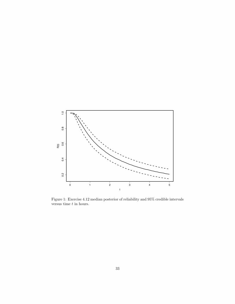
4.12 A 95% credible interval for µ is (2.65, 6.29) with a posterior median of3.81. A 95% credible interval for λ is (1.01, 2.27) with a posterior medianof 1.57. Using K = 5 equal probability bins, we find that 0.7% of theRB test statistics exceed the 0.95 quantile of the ChiSquared(4) referencedistribution, which suggests no lack of fit. See the plot of the posteriormedian of reliability with 90% credible interval over the first 5 hours inFigure 1.
4.13 Using K = 5 equal probability bins, we find that 4.9% of the RB teststatistics exceed the 0.95 quantile of the ChiSquared(4) reference distri-bution, which suggests no lack of fit. The DIC for the hierarchical model is245.446 and the DIC for the constant failure probability model is 285.322.Based on DIC, we prefer the hierarchical model. We provide the Win-BUGS code for the hierarchical in Table ??.
31

Table 1: WinBUGS code for exercise 4.13
########################################################## Exercise 4.13# EDG Hierarchical Model# for success probabilities pi[]# x[] number of failures in n[] trials
model{for( i in 1 : N ) {z[i]<-ind[i]y[i]<-n[i]-x[i]y[i] ~ dbin(pi[i],n[i])pi[i] ~dbeta(delta,gamma)I(.0001,.9999)}
#use InverseGammadelta<-1/rdeltagamma<-1/rgammardelta ~ dgamma(0.1,0.1)I(.001,1000)rgamma ~ dgamma(0.1,0.1)I(.001,1000)
}
Data
list(N = 63)
Inits
list(rdelta=.003,rgamma=.5,pi=c(.5,.5,.5,.5,.5,.5,.5,.5,.5,.5,.5,.5,.5,.5,.5,.5,.5,.5,.5,.5,.5,.5,.5,.5,.5,.5,.5,.5,.5,.5,.5,.5,.5,.5,.5,.5,.5,.5,.5,.5,.5,.5,.5,.5,.5,.5,.5,.5,.5,.5,.5,.5,.5,.5,.5,.5,.5,.5,.5,.5,.5,.5,.5))#########################################################
32
0 1 2 3 4 5
0.2
0.4
0.6
0.8
1.0
t
R(t)
Figure 1: Exercise 4.12 median posterior of reliability and 95% credible intervalsversus time t in hours.
33

Chapter 5
5.1 Draw a reliability block diagram describing how to successfully perform aneveryday task.
Consider the task of brushing your teeth. The following is a list of possiblecomponents for the block diagram:
1. get toothbrush
2. put toothpaste on toothbrush
3. put water on toothbrush
4. brush teeth
5. brush tongue
6. spit out toothpaste
7. rinse mouth
8. rinse toothbrush
Below is the reliability block diagram.
!
"
" #
$
%
%
$& ' (
! " $ % & ' (
)*+,-.,+,/012+34516,-78-91:38128;<=,>71?**/=
This a series system. Notice that component 3 is not essential for thecleaning of one’s teeth, so it can be left out of the diagram.
For additional reading om the diagrams discussed in this chapter I recom-mend System Reliability Theory by Rausand and Høyland.
5.2 Draw the reliability block diagram and fault tree corresponding to a 3-of-5system.
34

!
!
!
!
!
! "
"
"
#
#
$
#
$
%
$
%
%
" # $
" # %
" $ %
# $ %
!" # $" # %" # $" ! %" ! %" $ $# ! %# !
&'(
%# ! %# !
5.3 Determine the structure function for a 3-of-5 system.
35

The structure for a k-of-n system is given by equation 5.1.
φ(x) = x1x2x3(1− x4)(1− x5) + x1x2x4(1− x3)(1− x5)+ x1x2x5(1− x3)(1− x4) + x1x3x4(1− x2)(1− x5)+ x1x3x5(1− x2)(1− x4) + x1x4x5(1− x2)(1− x3)+ x2x3x4(1− x1)(1− x5) + x2x3x5(1− x1)(1− x4)+ x2x4x5(1− x1)(1− x3) + x3x4x5(1− x1)(1− x2)+ x1x2x3x4(1− x5) + x1x2x3x5(1− x4)+ x1x2x4x5(1− x3) + x1x3x4x5(1− x2)+ x2x3x4x5(1− x1) + x1x2x3x4x5
= x1x2x3 + x1x2x4 + x1x2x5 + x1x3x4 + x1x3x5 + x1x4x5
+x2x3x4 + x2x3x5 + x3x4x5 − 3x1x2x3x4 − 3x1x2x3x5
−3x1x2x4x5 − 3x1x3x4x5 − 3x2x3x4x5 + 6x1x2x3x4x5
5.4 Draw the reliability block diagram corresponding to Fig. 5.9.
Using the 5 minimal cut sets we might draw the block diagram as
!
"
#
$
%
! "$
! # "
#
%
&'()*+,-./0.1+2(0+3-/+%45
!
$
#
"
%
!
! $
#
%
#
"
%
&'()*+,-./0.1+2(0+3-/+%45
5.5 Determine the minimal path sets and minimal cut sets for IE6 in Fig. 5.9.Calculate the structure function for IE6.
The minimal cut sets are {BE2, BE3, BE5}, {BE3, BE4, BE5}. The mini-mal path sets are {BE2, BE4}, {BE3}, {BE5}. To determine the structurefor IE6 we can use either equations 5.3 or 5.4. Using equation 5.4 with the3 minimal path sets we get
φ(x) = 1− (1− x2x4)(1− x3)(1− x5)= x3 + x5 + x2x4 − x3x5 − x2x3x4 − x2x4x5 + x2x3x4x5
5.6 Define the structural importance of component i in a coherent system of ncomponents as
Iφ(i) =1
2n−1
∑x | xi=1
[φ(1i,x)− φ(0i,x)].
36

The sum is over the 2n−1 vectors for which xi = 1. Calculate the structuralimportance of each component in Fig. 5.5.
For component 1
(·, x2, x3) φ(1, x2, x3)− φ(0, x2, x3)(·00) 0(·01) 1(·10) 1(·11) 1
Iφ(1) =3
23−1=
34
For component 2
(x1, ·, x3) φ(x1, 1, x3)− φ(x1, 0, x3)(0·0) 0(0·1) 0(1·0) 1(1·1) 0
Iφ(2) =14
For component 3
(x1, x2, ·) φ(x1, x2, 1)− φ(x1, x2, 0)(00·) 0(01·) 0(10·) 1(11·) 0
Iφ(3) =14
5.7 Derive Eq. 5.8 from Eq. 5.1 by assuming that each component has reliabil-ity Ri(t) = R(t).
Beginning with equation (5.1),
P (φ(x) = 1) = P (∑j
(∏i∈Aj
xi)[∏i∈Acj
(1− xj)] = 1)
37

We want to choose the subset Aj that is a minimum path set (i.e. φ(x) = 1for the elements in Aj). Therefore, we want at least k elements of Aj to be1. Let s be the number of elements in Aj equal to 1. Therefore,
P ((∏i∈Aj
xi)[∏i∈Acj
(1−xj)] = 1) = P (s ≥ k) =n∑s=k
(ns )R(t)s(1−R(t))n−s = · · ·
· · · = 1−k−1∑s=0
(ns )R(t)s(1−R(t))n−s
5.8 Calculate the hazard function for a series system with n components wheneach component lifetime has a Weibull distribution.
Let Ci ∼Weibull(λi, βi). By definition, the hazard function ishs(t) = fs(t)
Rs(t). Using example 5.6 and Rs =
∏ni=1Ri, the hazard function is
hs(t) =∑ni=1 λiβit
βi−1i
5.9 Show that the mean time to failure (MTTF) for a standby system withperfect switching is equal to the sum of the MTTFs for each component:
MTTFS =n∑i=1
MTTFi.
MTTFs = E[Ts] = E[T1 + T2 + · · ·+ Tn] = E[T1] + E[T2] + · · ·+ E[Tn] =∑ni=1MTTFi
5.10 Suppose that each of the n components of a standby system with perfectswitching has an Exponential(λ) distribution. Show that the lifetime of thesystem has a Gamma(n, λ) distribution.
Ti ∼ Exponential(λ) = Gamma(1, λ). Let Ts denote the systems life-time. Then Ts =
∑ni=1 Ti. Therefore, since Ts is the sum of independent
Gamma(1, λ) random variables and using the result for gamma random vari-ables in section B of the appendix, we have Ts ∼ Gamma(n, λ).
5.11 Reanalyze the data from Table 5.3 assuming that the prior distribution forthe reliability of each component is [Γ(1/3)]−1(− log(πi))−
23 .
The posterior now becomes
p(π1, π2, π3 | x) ∝ π81(1− π1)2π7
2(1− π2)2π33(1− π3)(π1π2π3)10(1− π1π2π3)2
[− log(π1)]−23 [− log(π2)]−
23 [− log(π3)]−
23
38

QuantilesParameter Mean St.Dev 0.025 0.050 0.500 0.950 0.975
π1 0.868 0.074 0.699 0.732 0.878 0.965 0.976π2 0.861 0.077 0.690 0.720 0.871 0.968 0.978π3 0.887 0.082 0.690 0.733 0.904 0.987 0.992πS 0.998 0.002 0.992 0.994 0.999 1.000 1.000
The following is a histogram of the posterior distribution on πs:
πS
Density
0.965 0.975 0.985 0.995
050
100150200250300350
mh <- function(theta, size, data){pi1 = theta[1]pi2 = theta[2]pi3 = theta[3]s = data[,2]f = data[,3]par = array(0, dim=c(size, 4))arate1 = 0; arate2 = 0; arate3 = 0post = function(theta){
p1 = theta[1]; p2 = theta[2]; p3 = theta[3]ps = theta[1]*theta[2]*theta[3]val = p1^s[1] * (1-p1)^f[1] * p2^s[2] * (1-p2)^f[2] * p3^s[3] *
(1-p3)^f[3] * ps^s[4] * (1-ps)^f[4] * (-log(p1))^(-2/3) *
39

(-log(p2))^(-2/3) * (-log(p3))^(-2/3)return(val)
}for(i in 1:size){
pi1.star = runif(1)r = post(c(pi1.star, pi2, pi3)) / post(c(pi1, pi2, pi3))u = runif(1) <= rarate1 = arate1 + upi1 = pi1.star*(u==1) + pi1*(u==0)pi2.star = runif(1)r = post(c(pi1, pi2.star, pi3)) / post(c(pi1, pi2, pi3))u = runif(1) <= rarate2 = arate2 + upi2 = pi2.star*(u==1) + pi2*(u==0)pi3.star = runif(1)r = post(c(pi1, pi2, pi3.star)) / post(c(pi1, pi2, pi3))u = runif(1) <= rarate3 = arate3 + upi3 = pi3.star*(u==1) + pi3*(u==0)pis = 1 - (1-pi1)*(1-pi2)*(1-pi3)par[i,] = c(pi1, pi2, pi3, pis)
}arate = c(arate1, arate2, arate3); arate = arate/sizelist = list(par = par, accept = arate)return(list)
}
start <- data[,2]/data[,4]sample <- mh(start[1:3], 10000, data)plot(as.mcmc(sample$par))
#get rid of burn-in samples - calculate summary statisticssample$par <- sample$par[-c(1:100),]mu <- array(apply(sample$par, 2, mean), dim=c(4,1))st.dev <- array(apply(sample$par, 2, sd), dim=c(4,1))quant = rbind(quantile(sample$par[,1], c(.025, .05,.5,.95,.975)),quantile(sample$par[,2], c(.025, .05,.5,.95,.975)),quantile(sample$par[,3], c(.025, .05,.5,.95,.975)),quantile(sample$par[,4], c(.025, .05,.5,.95,.975)))summary = array(c(mu, st.dev, quant), dim=c(4,7))colnames(summary) <- c("Mean", "Std Dev", "2.5%", "5%", "50%","95%", "97.5%")rownames(summary) <- c("pi1", "pi2", "pi3", "piS")summaryhist(sample$par[,4], freq=F, xlab=expression(pi[S]), main="")
40

5.12 There are a variety of different measures of the reliability importance of acomponent (Rausand and Høyland, 2003). Birnbaum’s measure of impor-tance of the ith component at time t is
IB(i | t) =dRS(t)dπi(t)
.
Birnbaum’s measure is the partial derivative of the system reliability withrespect to each component reliability πi(t). A larger value of IB(i | t) meansthat a small change in the reliability of the ith component results in acomparatively large change in the system reliability. Show that in a seriessystem, Birnbaum’s measure selects the component with the lowest reliabil-ity as the most important one.
The three Birnbaum’s measures are: IB1 = π2π3, IB2 = π1π3, and IB3 =π1π2. Without loss of generality, suppose π1 < π2 < π3. Based on the de-scription of the measure in the exercise, we are looking for the largest value,which should correspond to π1. Therefore, by comparing the different mea-sures: IB1 = π2π3 > π1π3 = IB2 if and only if π2 > π1. Which is true byour assumption. Also, IB1 = π2π3 > π1π2 = IB3 if and only if π3 > π1.Which is again true by our assumption. Therefore, IB1 is the largest valueand the procedure selected the most important component. This result stillholds if π1 ≤ π2 < π3. It is trivial for the case that π1 = π2 = π3.
5.13 Show how to calculate the posterior distribution for π1, π2, and π3 using thedata in Table 5.1 using simulation and the Metropolis-Hastings algorithm.
R code for a Metropolis-Hastings algorithm:
mh <- function(theta, size, data){pi1 = theta[1]pi2 = theta[2]pi3 = theta[3]s = data[,2]f = data[,3]par = array(0, dim=c(size, 3))arate1 = 0; arate2 = 0; arate3 = 0post = function(theta){
p1 = theta[1]; p2 = theta[2]; p3 = theta[3]val = p1^s[1]*(1-p1)^f[1]*p2^s[2]*(1-p2)^f[2]*p3^s[3]*(1-p3)^f[3]return(val)
}for(i in 1:size){
pi1.star = runif(1)r = post(c(pi1.star, pi2, pi3)) / post(c(pi1, pi2, pi3))
41

u = runif(1) <= rarate1 = arate1 + upi1 = pi1.star*(u==1) + pi1*(u==0)pi2.star = runif(1)r = post(c(pi1, pi2.star, pi3)) / post(c(pi1, pi2, pi3))u = runif(1) <= rarate2 = arate2 + upi2 = pi2.star*(u==1) + pi2*(u==0)pi3.star = runif(1)r = post(c(pi1, pi2, pi3.star)) / post(c(pi1, pi2, pi3))u = runif(1) <= rarate3 = arate3 + upi3 = pi3.star*(u==1) + pi3*(u==0)par[i,] = c(pi1, pi2, pi3)
}arate = c(arate1, arate2, arate3); arate = arate/sizelist = list(par = par, accept = arate)return(list)
}
start <- data[,2]/data[,4]sample <- mh(start, 10000, data)#get rid of burn-in and calculate summary statisticsplot(as.mcmc(sample$par))sample$par <- sample$par[-c(1:50),]mu <- array(apply(sample$par, 2, mean), dim=c(4,1))st.dev <- array(apply(sample$par, 2, sd), dim=c(4,1))quant = rbind(quantile(sample$par[,1], c(.025, .05,.5,.95,.975)),
quantile(sample$par[,2], c(.025, .05,.5,.95,.975)),quantile(sample$par[,3], c(.025, .05,.5,.95,.975)),quantile(sample$par[,4], c(.025, .05,.5,.95,.975)))
summary = array(c(mu, st.dev, quant), dim=c(4,7))colnames(summary) <- c("Mean", "Std Dev", "2.5%", "5%", "50%", "95%", "97.5%")rownames(summary) <- c("pi1", "pi2", "pi3", "piS")summaryhist(sample$par[,4], freq=F, xlab=expression(pi[S]),
main="Marginal Posterior Distribution from M-H")
The posterior distributions can be found in Table 5.2 and Fig. 5.15.
R code for a simulation:
sim <- function(size){pi1 = rbeta(size, 9,3)pi2 = rbeta(size, 8,3)pi3 = rbeta(size, 4,2)pis = pi1*pi2*pi3
42

pi = array(c(pi1,pi2,pi3, pis), dim=c(size,4))mu <- array(apply(pi, 2, mean), dim=c(4,1))st.dev <- array(apply(pi, 2, sd), dim=c(4,1))quant = rbind(quantile(pi[,1], c(.025, .05,.5,.95,.975)),
quantile(pi[,2], c(.025, .05,.5,.95,.975)),quantile(pi[,3], c(.025, .05,.5,.95,.975)),quantile(pi[,4], c(.025, .05,.5,.95,.975)))
summary = array(c(Mean=mu, Std.Dev=st.dev, quant), dim=c(4,7))colnames(summary) <- c("Mean", "Std Dev", "2.5%", "5%", "50%",
"95%", "97.5%")rownames(summary) <- c("pi1", "pi2", "pi3", "piS")list = list(pi = pi, summary = summary)
}simulation <- sim(10000)simulation$summaryhist(simulation$pi[,4], freq=F, xlab=expression(pi[S]),
main="Marginal Distribution from Simulation")
QuantilesParameter Mean St.Dev 0.025 0.050 0.500 0.950 0.975
π1 0.750 0.119 0.494 0.536 0.762 0.920 0.941π2 0.726 0.128 0.448 0.495 0.738 0.915 0.936π3 0.673 0.177 0.289 0.347 0.696 0.925 0.947πS 0.366 0.133 0.132 0.161 0.359 0.600 0.645
5.14 Assume a two-component series system. One component has an Exponen-tial(3) prior distribution; the other has a Weibull(5, 2) prior distribution.Using simulation, determine the probability density function of the priordistribution for the system.
r1 = rexp(10000, 3)r2 = rweibull(10000, 5,2)rs = r1*r2hist(rs, freq=F, xlab = expression(R[S]), main="")mean(rs); sd(rs)quantile(rs, c(.025, .05,.5,.95,.975))
QuantilesParameter Mean St.Dev 0.025 0.050 0.500 0.950 0.975
RS 0.609 0.652 0.015 0.030 0.405 1.88 2.340
43

RS
Density
0 2 4 6 8 10
0.0
0.2
0.4
0.6
0.8
1.0
5.15 Translate the fault tree in Fig. 5.9 into a BN.
44

!"
#$%&'(')*
+",
+"-
+".
+"/
0"/ 0"% 0",
0"#+"#
+"%
0"-
012'341)&5'*6789&:78&;4<=&-=>
5.16 Translate the fault tree in Fig. 5.24 into a BN. Write down the conditionalprobabilities specified by the fault tree.
!
"#$%&'( )#$%&'(
" *") )
)%+,(&%-#.,/0123#14#$&56#7689
45

P(BF = 0 |CAB = 0, B = 0) = 1 P(AF = 0 |CAB = 0, A = 0) = 1P(BF = 0 |CAB = 1, B = 0) = 1 P(AF = 0 |CAB = 1, A = 0) = 1P(BF = 0 |CAB = 0, B = 1) = 1 P(AF = 0 |CAB = 0, A = 1) = 1P(BF = 0 |CAB = 1, B = 1) = 0 P(AF = 0 |CAB = 1, A = 1) = 0
P(D = 0 |AF = 0, BF = 0) = 1P(D = 0 |AF = 1, BF = 0) = 0P(D = 0 |AF = 0, BF = 1) = 0P(D = 0 |AF = 1, BF = 1) = 0
5.17 Suppose that the data in Table 5.3 come from a three-component paral-lel system. Using independent Uniform(0, 1) prior distributions for thereliability of each component, calculate the posterior distributions for thereliability of each component and the system.
The formula for the reliability of the system in a parallel system is given onpage 136. For the three component system in Table 5.3, we have
πS = 1− (1− π1)(1− π2)(1− π3)
The MCMC algorithm is similar to the one used in problems 11 and 13.Only the posterior function needs to be adjusted.
QuantilesParameter Mean St.Dev 0.025 0.050 0.500 0.950 0.975
π1 0.841 0.078 0.669 0.696 0.850 0.953 0.962π2 0.834 0.081 0.655 0.684 0.845 0.948 0.959π3 0.845 0.092 0.624 0.676 0.858 0.968 0.978πS 0.996 0.004 0.986 0.989 0.997 1.000 1.000
Notice the difference between the posterior distribution for the reliabilityof this parallel system and the series system from the same data shown inTable 5.4.The Kernel density estimates of the posterior distributions of the compo-nents and the system are shown below.
46

0.4 0.6 0.8 1.0
012345
π1
Density
0.4 0.6 0.8 1.0
01
23
4
π2
Density
0.4 0.6 0.8 1.0
01
23
4
π3
Density
0.94 0.96 0.98 1.00
050
150
πS
Density
5.18 Suppose that we have a three-component system like that in Example 5.1,and suppose that each component has an Exponential(λ) lifetime. Write anexpression for the probability density function of the lifetime of the system.
fi(t |λ) = λe−λt Fi(t |λ) = 1− e−λt
The reliability of the system can be derived combining equations 5.5 and5.7.
RS(t) = R1(1− (1−R2)(1−R3))= R1R2 +R2R3 −R1R2R3
= 2R2 −R3 (since R1 = R2 = R3)1− Fs(t) = 2(1− F (t))2 − (1− F (t))3
d
dt(1− Fs(t)) =
d
dt
[1− F (t)− F 2(t) + F 3(t)
]fs(t) = f(t) + 2f(t)F (t)− 3f(t)F 2(t)
= λe−λt + 2λe−λt(1− e−λt)− 3λe−λt(1− e−λt)2
= 4λe−2λt − 3λe−3λt
47

5.19 Reanalyze the BN in Fig. 5.22 with data from Tables 5.8 and 5.9 assumingthat we have also observed 20 observations with C1 = 0, C2 = 1, C3 = 1that resulted in 6 system successes and 14 system failures.
We this information we can add π6FSS(1−πFSS)14 to the likelihood and the
posterior becomes
p(π1, π2, π3 | x) ∝ π81(1− π1)2π7
2(1− π2)2π33(1− π3)π6
FSS(1− πFSS)14π10S (1− πS)2
[− log(π1)]−23 [− log(π2)]−
23 [− log(π3)]−
23
I[πFSS ∈ (0.35, 0.85)]
Using the Metropolis-Hastings algorithm given below we obtain
QuantilesParameter Mean St.Dev 0.025 0.050 0.500 0.950 0.975
π1 0.82 0.10 0.59 0.63 0.83 0.95 0.97π2 0.78 0.12 0.51 0.56 0.80 0.95 0.96π3 0.78 0.16 0.41 0.47 0.80 0.97 0.98πFSS 0.42 0.06 0.35 0.35 0.41 0.54 0.57πS 0.80 0.05 0.68 0.71 0.81 0.88 0.89
With this new information the 95% credible interval for πFSS has narrowedfrom (.36, 0.84) in the example in the text to (0.35, 0.57).
mh <- function(theta, size, data){pi1 = theta[1]pi2 = theta[2]pi3 = theta[3]pifss = theta[4]s = data[,2]f = data[,3]par = array(0, dim=c(size, 5))arate1 = 0; arate2 = 0; arate3 = 0; arate4 = 0post = function(theta){
p1 = theta[1]; p2 = theta[2]; p3 = theta[3]; pFSS = theta[4]ps = 0.95*p1*p2*p3 + 0.8*p1*p2*(1-p3) + 0.85*p1*(1-p2)*p3 +
0.5*p1*(1-p2)*(1-p3) + pFSS*(1-p1)*p2*p3 + 0.4*(1-p1)*p2*(1-p3) + 0.55*(1-p1)*(1-p2)*p3 + 0.05*(1-p1)*(1-p2)*(1-p3)
val = p1^s[1] * (1-p1)^f[1] * p2^s[2] * (1-p2)^f[2] * p3^s[3] *(1-p3)^f[3] * pFSS^6 * (1-pFSS)^14 * ps^s[4] *(1-ps)^f[4] * (-log(p1))^(-2/3) * (-log(p2))^(-2/3) *(-log(p3))^(-2/3)
return(val)}
48

for(i in 1:size){pi1.star = runif(1)r = post(c(pi1.star, pi2, pi3, pifss)) /
post(c(pi1, pi2, pi3, pifss))u = runif(1) <= rarate1 = arate1 + upi1 = pi1.star*(u==1) + pi1*(u==0)pi2.star = runif(1)r = post(c(pi1, pi2.star, pi3, pifss)) /
post(c(pi1, pi2, pi3, pifss))u = runif(1) <= rarate2 = arate2 + upi2 = pi2.star*(u==1) + pi2*(u==0)pi3.star = runif(1)r = post(c(pi1, pi2, pi3.star, pifss)) /
post(c(pi1, pi2, pi3, pifss))u = runif(1) <= rarate3 = arate3 + upi3 = pi3.star*(u==1) + pi3*(u==0)pifss.star = runif(1,.35,.85)r = post(c(pi1, pi2, pi3, pifss.star)) /
post(c(pi1, pi2, pi3, pifss))u = runif(1) <= rarate4 = arate4 + upifss = pifss.star*(u==1) + pifss*(u==0)pis = 0.95*pi1*pi2*pi3 + 0.8*pi1*pi2*(1-pi3) + 0.85*pi1*
(1-pi2)*pi3 + 0.5*pi1*(1-pi2)*(1-pi3) + pifss*(1-pi1)*pi2*pi3 + 0.4*(1-pi1)*pi2*(1-pi3) + 0.55*(1-pi1)*(1-pi2)*pi3 + 0.05*(1-pi1)*(1-pi2)*(1-pi3)
par[i,] = c(pi1, pi2, pi3, pifss, pis)}arate = array(c(arate1, arate2, arate3, arate4), dim=c(1,4))colnames(arate) = c("pi1", "pi2", "pi3", "piFSS")arate = arate/sizereturn(list(par = par, accept = arate))
}start <- c(data[1:3,2]/data[1:3,4], 6/14)sample <- mh(start, 10000, data)
5.20 In Example 5.7, determine the probability that the item fails because of risk1.
49

The probability that the item fails because of risk 1 is given by
P(T1 < T2) =∫ ∞
0
P(T2 > t |T1 = t)fT1dt
=∫ ∞
0
e−λ2tλ1e−λ1tdt
= λ1
∫ ∞0
e−t(λ1+λ2)dt
=λ1
λ1 + λ2
50

Solutions to Selected Chapter 6 Exercises
6.1 From Λ(Ti)− Λ(Ti−1) ∼ Exponential(1), where Λ(Ti) = λTi for the expo-nential renewal process, we obtain Λ(Ti)−Λ(Ti−1) = λTi−λTi−1 = λ(Ti−Ti−1) ∼ Exponential(1). Consequently, Ti − Ti−1 ∼ 1
λExponential(1) =Exponential(λ).
6.2 For failure times t1, t2, . . . , tn, T1, T2−T1, . . . , Tn−Tn−1 are i.i.d.Gamma(α, λ).The corresponding likelihood is proportional to
[λα/Γ(α)]n(
n∏i=1
(ti − ti−1)α−1
)exp(−λtn) ,
where t0 = 0. Under Type-I censoring at tc, the corresponding likelihoodis proportional to
[λα/Γ(α)]n(
n∏i=1
(ti − ti−1)α−1
)exp(−λtn)
∫ ∞tc−tn
f(t|α, λ)dt ,
where f(t|α, λ) is the Gamma(α, λ) probability density function. Type-IIcensoring is not relevant for a single repairable system.
6.4 A 95% credible interval for κ is (0.473, 1.120), so that the data suggestthat there is no need to use the MPLP over the PLP, where κ equals 1.Accounting for the censored observation, 260.4 ≈ 4. Using K = 4 equalprobability bins, we find that 1.3% of the RB test statistics exceed the0.95 quantile of the ChiSquared(3) reference distribution, which suggestsno lack of fit.
6.8 If the last failure occurred at t∗, we have Λ(T + t∗)−Λ(t∗) ∼ Gamma(κ, 1)so that Rt∗(t) = P(T > t), but
T > t ≡ Λ−1 (Λ(t∗) +X)− t∗ > t ≡ X > Λ(t+ t∗)− Λ(t∗) ,
where X ∼ Gamma(κ, 1). Consequently,
Rt∗(t) =∫ ∞
Λ(t+t∗)−Λ(t∗)
f(x|κ, 1)dt ,
where f(x|κ, 1) is the Gamma(κ, 1) probability density function.
6.20 Assuming that uptime U ∼ Gamma(αU , λU ) and downtimeD ∼ Gamma(αD, λD),then the long-run availability A = E(U)
E(U)+E(D) is
αU/λUαU/λU + αD/λD
.
51

Solutions to Selected Chapter 7 Exercises
7.2 We fit a logistic regression model in heating time and soaking time. Weuse the actual heating and soaking times (centered by their respective av-erages) as covariates in a full second order model, i.e., X1, X2, X1X2, X2
1 ,and X2
2 , where X1 and X2 are the centered heating and soaking times, re-spectively. The regression coefficient of X2 has a high posterior probability(0.992) of being different from zero, i.e., has an impact. The coefficientsfor X2
2 , X21 , and X1X2 are less important with posterior probabilities of
0.938, 0.920, and 0.908, respectively, of being different from zero. Seethe following reference for more details: B.P. Weaver and M.S. Hamada(2008), “A Bayesian Approach to the Analysis of Industrial Experiments:An Illustration with Binomial Count Data,” Quality Engineering, 20, 269–280.
7.3 Using K = 4 ≈ 630.4 equal probability bins, we find that 4.3% of theRB test statistics exceed the 0.95 quantile of the ChiSquared(3) referencedistribution, which suggests no lack of fit.
7.14 a) We fit the modelYi ∼ Poisson(λiti) ,
where
log(λi) = β1 + β2SY S2i + β3SY S3i + β4SY S4i + β5SY S5i+β6OTY 2i + β7OTY 3i + β8OTY 4i+β9V TY 2i + β10V TY 3i + β11V TY 4i + β12V TY 5i + β13V TY 6i+β14SIZ2i + β15SIZ3i + β16OPM2i .
The covariates in the Poisson regression model above are dummy vari-ables, e.g., SY S2i = 1 if SY S = 2, etc. The summaries of the posteriordistributions for the βs are given in the table below.
b) A 90% credible upper bound on the predicted number of failures inthe next 10 years for a normally closed (OPM=1) 2- 10-inch (SIZ=2)air-driven (OTY=1) globe valve (VTY=5) in a power conversion system(SYS=3) is 99.
52

QuantilesParameter Mean Std Dev 0.025 0.500 0.975
β1 -10.000 0.781 -11.740 -9.971 -8.618β2 0.9023 0.5226 -0.1079 0.8903 1.9800β3 1.030 0.490 0.121 1.012 2.065β4 1.214 0.551 0.161 1.204 2.343β5 0.317 0.572 -0.766 0.311 1.469β6 0.5966 0.5961 -0.6806 0.6254 1.6900β7 -1.213 0.248 -1.700 -1.211 -0.719β8 -2.560 0.497 -3.610 -2.529 -1.672β9 0.2025 0.7742 -1.3010 0.1882 1.7550β10 0.6059 0.7904 -0.9477 0.6105 2.1500β11 3.068 0.592 2.040 3.026 4.370β12 1.893 0.602 0.825 1.846 3.203β13 0.833 0.992 -1.246 0.875 2.677β14 -0.0039 0.2792 -0.5266 -0.0069 0.5741β15 1.625 0.316 1.021 1.618 2.262β16 -0.2065 0.1896 -0.5760 -0.2063 0.1617
7.17 For X ∼ Gamma(α, λ), we can use Y = λX to remove λ as seen byY ∼ Gamma(α, 1). However, we cannot transform Y to remove α. Con-sequently, a Cox-Snell residual does not exist for the gamma distribution.The deviance residual for the ith observation yi has the form:
sign(yi − µi)√
2[− log(yi − µi) + (yi − µi)/µi] ,
where µi = αi/λ2i . See McCullagh and Nelder (1989) for more details.
7.24 Based on the predictive distribution summaries displayed in the table be-low, PCB type copper-tin-lead at 20◦C is the recommended factor-levelcombination with the longest lifetime distribution.
QuantilesPCB Type Temp (◦ C) 0.025 0.500 0.975
copper-nickel-tin 20 251.2 700.2 1233.260 55.0 157.9 278.5
100 51.6 143.9 253.3copper-nickel-gold 20 570.5 1636.9 2869.4
60 89.8 533.9 929.1100 142.3 403.6 708.6
copper-tin-lead 20 587.4 1702.2 3031.960 168.1 469.5 844.3
100 130.5 372.8 646.8
53

Solutions to Selected Chapter 8 Exercises
8.1 We use the model yij = −5 + βixj + ε, where βi ∼ Normal(µβ , σ2β) and
ε ∼ Norma(0, σ2), for the jth observation of the ith LED. See the tablebelow for posterior summaries of the model parameters. Using K = 5equal probability bins, we find that 33.6% of the RB test statistics exceedthe 0.95 quantile of the ChiSquared(4) reference distribution, which sug-gests some lack of fit. Using a threshold of -2.0 at 300 hours, a 90% credibleinterval for reliability is (0.3343, 0.7514) with a posterior median of 0.5505.
QuantilesParameter Mean Std Dev 0.025 0.500 0.975β1 0.004246 5.482E-4 0.003169 0.004245 0.005317β2 0.007738 5.528E-4 0.006640 0.007746 0.008833β3 0.007844 5.571E-4 0.006747 0.007838 0.008937β4 0.007461 5.543E-4 0.006385 0.007464 0.008572β5 0.009606 5.523E-4 0.008527 0.009608 0.010710β6 0.006429 5.500E-4 0.005347 0.006427 0.007494β7 0.007638 5.613E-4 0.006531 0.007635 0.008756β8 0.008719 5.525E-4 0.007629 0.008722 0.009819β9 0.011470 5.591E-4 0.010380 0.011470 0.012580µβ 0.007862 0.006230 -0.004482 0.007914 0.020440σ 0.203600 0.024980 3.036E-4 0.200900 0.260200σβ 0.017710 0.005276 0.010830 0.016750 0.030620
8.4 Using K = 9 equal probability bins, we find that 32.5% of the RB teststatistics exceed the 0.95 quantile of the ChiSquared(8) reference distri-bution, which shows lack of fit, as compared with the original model inExample 8.2, whose assessment is given below as the solution to Exer-cise 8.16. Consequently, we prefer the original model and do not use thealternative model to calculate R(t) and t0.1.
8.14 Using K = 22 equal probability bins, we find that 3.8% of the RB teststatistics exceed the 0.95 quantile of the ChiSquared(21) reference distri-bution, which suggests no lack of fit.
54

8.16 Here, we consider only the fit of the model in Example 8.2. Using K = 9equal probability bins, we find that 12.9% of the RB test statistics ex-ceed the 0.95 quantile of the ChiSquared(8) reference distribution, whichsuggests no lack of fit.
8.17 It is doubtful that there is a closed form expression for the destructivemeasurement zi = Di(t) with Di(t) defined in Eq. 8.21 when it is measuredwith a Normal(0, σ2) measurement error. Instead, we derive Eq. 8.23, theprobability density function of zi without measurement error as follows.We have z = D(t) = β0 − β1(1/x)t, where x ∼ Lognormal(µ, σ2), wherethe probability density function of x is
f(x |µ, σ2) =1
x√
2πσ2exp
[− 1
2σ2(log(x)− µ)2
].
We obtain the probability desntiy function of z by a change of variables.Because x can be expressed in terms of z by x = β1t
β0−z , we see thatdx = β1t
(β0−z)2 dz. Consequently,
f(z |µ, σ2, β0, β1, t) =(β1t)
(β0 − z)2
1β1tβ0−z
√2πσ2
exp
[− 1
2σ2
(log(
β1t
β0 − z
)− µ
)2].
which simplifies to Eq. 8.23.
55

Selected Solutions to Chapter 9 Exercises
9.1 Under a Beta(1, 1) prior, the 0.90 posterior quantile of the 95% credibleinterval length for a sample size of 377 is 0.075. The 0.90 posterior quantileof the 95% credible interval length for a sample size of 3000 is 0.036, sothat we use nmax = 3000. A bisection search finds that for a sample sizeof 2695, the 0.90 posterior quantile of the 95% credible interval length doesnot exceed 0.0375. That is noptimal = 2695.
9.2 For (a) 5 out of 10 successes, noptimal = 1531; (b) 50 out of 100 successes,noptimal = 1462; (c) 9 out of 10 successes, noptimal = 1219; and (d) 90 outof 100 successes, noptimal = 643.
9.3 Under X ∼ Poisson(λt), with a Gamma(1, 1) prior for λ, α = 0.95, γ =0.90, Ltarget = 0.05, and tmax = 100000, we find using a bisection searchthat toptimal = 14339. We can carry out the testing by allocating the totaltesting time of 14339 across multiple units that can be tested simultaneously,assuming that all the test units have a common λ.
9.4 Consider the data collection planning example, which focuses on reliabilityat time t = 24 months. Assuming that the lifetimes have a LogNormal(µ, σ2)distribution, we use the following prior distributions: µ ∼ Normal(4, 0.1)and σ2 ∼ InverseGamma(20, 10). Letting γ = 0.90, α = 0.95, andLtarget = 0.1, we find that a sample size nmax = 500 meets the statedrequirement, i.e., the probability of the α × 100% credible interval lengthof R(24) not exceeding Ltarget is at least γ. A bisection search yieldsnoptimal = 83. The example in the chapter used prior distributions, whichyielded a reliability prior distribution at 24 months with a median of 0.50and a 0.95 probability interval of (0.00, 1.00). The prior distributions usedin this exercise yielded a reliability prior distribution at 24 months with amedian of 0.88 and a 0.95 probability interval of (0.79, 0.94).
9.7 We use the following less diffuse priors distributions:
β0 ∼ Normal(−7.3, (0.15/5)2),β1 ∼ Normal(7.5, (0.15/5)2), andσ2 ∼ InverseGamma(100× 5, 0.112 × 100× 5).
For γ = 0.9, α = 0.95, Ltarget = 0.1, and reliability at time t = 10,500 days,we check to make sure that the planning criterion for ni = 400, i = 1, 2, 3and v2 = 0.5 meets the requirement. We use a GA that minimizes the totalsample size, n1 + n2 + n3, where instead of discarding (n1, n2, n3) cases,which have a planning criterion ρ (i.e., the probability that the α × 100%credible interval length does not exceed Ltarget) that does not exceed γ, wepenalize these cases by minimizing:
n1 + n2 + n3 + [100(γ − ρ)/0.01]I(ρ < γ) + [25(γ − ρ)/0.01]I(ρ > γ).
56

A GA found the nearly optimal solution v2,optimal = 0.496 and noptimal =(n1, n2, n3), where n1 = 145, n2 = 50, and n3 = 189, whose penalizedcriterion is 384.
57