Chapter 1 Introduction - KFUPM

i

ii

iii

STARTING BY THE NAME OF ALLAH

THE MOST BENEFICIAL AND THE MOST MERCIFUL

iv

Dedicated to

My beloved parents,

My Wife

and

My daughter

v

ACKNOWLEDGEMENT

“In the name of Allah, The Most Gracious and The Most Merciful”

All praise belongs to Almighty Allah (s.w.t.) for bestowing me with courage and

perseverance to carry out this work sincerely. I thank Almighty Allah for giving me

chance to do my M.S. successfully at King Fahd University of Petroleum and Minerals,

Dhahran. I am happy to have had a chance to glorify His name in the sincerest way

through this small accomplishment and ask Him to accept my efforts.

My deep gratitude and appreciation goes to my thesis advisor, Dr. Rached Ben Mansour

for his constant endeavor, guidance and motivation during the course of my study. His

valuable and priceless suggestions made this work interesting and challenging for me. I

also wish to express my deep appreciation to Dr. M A Habib and Dr. S. A. Said for their

help, guidance, and constant encouragement during my M.S.

Last but not the least I would like to thank Dr. Klas Andersson for his cooperation and

encouragement. His comments and contributions are highly appreciated.

vi

TABLE OF CONTENTS ACKNOWLEDGEMENT……………………………………………………………….v

LIST OF TABLES…………………………………………………………………….....ix

LIST OF FIGURES……………………………………………………………………....x

LIST OF ABBREVIATIONS…………………………………………………………..xv

THESIS ABSTRACT (ENGLISH)……………………………………………………..xvi

THESIS ABSTRACT (ARABIC)……………………………………………………...xvii

CHAPTER 1………………………………………………………………………………1 INTRODUCTION………………………………………………………………………...1

1.1 Research Background………………………………………………………....1

1.2 Problem Statement……………………………………………………….........5

1.3 Objectives……………………………………………………………………..6

1.4 Thesis Outline…………………………………………………………………7

CHAPTER 2………………………………………………………………………………8 CARBON CAPTURE TECHNOLOGIES……………………………………………….8

2.1 Post-Combustion Capture (PCC) Technology………………………………...8

2.2 Pre-Combustion Capture Technology…………………………………………9

2.3 Oxy-Fuel Combustion………………………………………………………..10

2.4 Literature review……………………………………………………………..11

CHAPTER 3……………………………………………………………………………..28

GAS RADIATION MODELS…………………………………………………………..28

3.1 Introduction………………………………………………………………….28

3.2 Radiative Transfer Equation (RTE)…………………………………….........30

vii

3.3 Radiative Transfer Equation (RTE) Solution Methods……………………...36

3.3.1 Introduction…………………………………………………...........36

3.3.2 Overview of computational methods in radiative transfer…………37

3.3.3 Discrete Ordinate Method (DO)…………………………………...39

3.4 Modeling of spectral nature of radiative transfer………………………........41

3.4.1 Introduction………………………………………………………..41

3.4.2 Narrow-band models………………………………………….........43

3.4.3 Wide-band models……………………………………………........44

3.4.4 Total absorptivity-emissivity models………………………………45

3.4.5 Absorption and emission coefficients……………………………...47

3.5 Simple grey gas model (SGG)………………………………………….........48

3.6 Exponential wide band model (EWBM)…………………………………….50

3.7 Leckner model……………………………………………………………….52

3.8 Perry model………………………………………………………………….55

3.9 Weighted sum of grey gas model (WSGG)…………………………………57

CHAPTER 4…………………………………………………………………………….62

GAS RADIATION MODELS VALIDATION FOR COMBUSTION

PROBLEM…………………….......................................................................................62

4.1 Introduction…………………………………………………………………62

4.2 Problem description…………………………………………………………63

4.3 Numerical simulation………………………………………………………..65

4.4 Results and Discussion…………………………………………………........67

viii

4.5 Assessment of gas radiation models……………………………………......75

CHAPTER 5……………………………………………………………………………85

CFD MODELING OF A WATER TUBE BOILER UNDER AIR

AND OXY-FUEL COMBUSTION……………………………………………………85

5.1 Introduction…………………………………………………………………85

5.2 Boiler description……………………………………………………….......85

5.3 Problem setup……………………………………………………………….88

5.4 Grid independence study……………………………………………………91

5.5 Results and discussions……………………………………………………...94

5.5.1 Comparisons between gas radiation models……………………....94

5.5.2 Characteristics of Oxyfuel and Air-Fuel Combustion

Processes………………………………………………………………..103

CHAPTER 6………………………………………………………………………........117

CONCLUSIONS AND RECOMMENDATIONS…………………………………….117

6.1 Conclusions………………………………………………………………....117

6.2 Recommendations for future work…………………………………………118

NOMENCLATURE……………………………………………………………….......120

REFERENCES…………………………………………………………………….......122

Vita……………………………………………………………………………………..128

ix

LIST OF TABLES

Table 1 Coefficients to calculate the H2O emissivity with M=3 and N=3………….......54

Table 2 Coefficients to calculate the CO2 emissivity with M=4 and N=5………….......54

Table 3 Pressure correction parameters used in equation (35) and equation (36)…........54

Table 4 Empirical constants used in equation (42)……………………………………...56

Table 5 Coefficients for the WSGG model [41]………………………………………...60

Table 6 Coefficients for the WSGG (4+1) model [26]………………………………….61

Table 7 Coefficients for the WSGG (3+1) model [26]………………………………….61

Table 8 Design data of boiler………………………………………………………........86

Table 9 Different grids of the furnace…………………………………………………...91

x

LIST OF FIGURES

Figure 1 CO2 emission level [1]……………………………………………………...........2

Figure 2 NO emission level [1]………………………………………………....................3

Figure 3 Principles of the three main CO2 capture options [2]……………………………4

Figure 4 Post-combustion capture (PCC) process [3]……………………………………..9

Figure 5 Pre-combustion capture process [3]…………………………………................10

Figure 6 Basic principle of oxyfuel technology [4]…………………………...................11

Figure 7 coordinates for derivation of the radiative transfer equation [54]……………..32

Figure 8 The Chalmers 100 kW O2/CO2 combustion test unit [42]……………………..64

Figure 9 fuel burner design [42]………………………………………………................65

Figure 10 Temperature profile at distance 0.384m from the burner with different radiation

models, air combustion…………………………………………………………………..69





Figure 13 CO2 concentrations at distance 1.4m from the burner,

air combustion…………………………………………………………………………...71

Figure 14 Temperature profile at distance 0.553 m for different radiation models, OF21

combustion………………………………………………………………………………72


models, OF21 combustion………………………………………….................................73

xi

Figure 16 CO2 concentrations at distance 0.384m from the burner, OF21

combustion………………………………………………………………………….........73


models, OF27 combustion……………………………………………………………….74

Figure 18 CO2 concentrations at distance 0.384m from the burner, OF27

combustion………………………………………………………………………….........75

Figure 19 Emissivity profiles as a function of gas temperature for different radiation






Figure 22 Discretization of a path length………………………………………………..80

Figure 23 Radiation intensity at distance 0.384m from the burner with different radiation



models, OF21 combustion………………………………………………………………82




models, air combustion………………………………………………………………….83

xii





Figure 29 Layout of furnace of the boiler………………………………………………86

Figure 30 Side view of Furnace of the boiler …………………………………………..87

Figure 31 burner construction…………………………………………………………..88

Figure 32 General view of the boiler…………………………………………………...89

Figure 33 Closer view of the burners……………………………………………….......90

Figure 34 Temperature profile at line (x=3.264, z=6) along Y-axis……………………92

Figure 35 Temperature profile at line (x=4.539, y=-2.135) along Z-axis………………93

Figure 36 Total heat flux profile at line (y=2, z=0) along X-axis………………………93

Figure 37 Total heat flux profile at line (x=0, y=3) along Z-axis………………………94

Figure 38 Temperature profile at line (x=4.539, y=4) along Z-axis,

air combustion…………………………………………………………………………..96

Figure 39 Temperature profile at line (x=3.264, y=-1.0675) along Z-axis, air

combustion……………………………………………………………………...............96

Figure 40 Temperature profile at line (x=4.539, y=4) along Z-axis, OF21

combustion……………………………………………………………………...............98

Figure 41 Temperature profile at line (x=3.264, y=-1.0675) along Z-axis, OF21

combustion………………………………………………………………………….........98

xiii

Figure 42 Temperature profile at line (x=3.264, y=-1.0675) along Z-axis, OF27

combustion………………………………………………………………………….. …..99

Figure 43 Temperature profile at line (x=4.539, y=4) along Z-axis, OF27

combustion………………………………………………………………………….......100

Figure 44 CO2 mole fraction profile at line (x=3.264, y=-1.0675) along Z-axis for

different radiation models, OF27 combustion……………………………….................101

Figure 45 H2O mole fraction profile at line (x=3.264, y=-1.0675) along Z-axis for

different radiation models, OF27 combustion………………………………………….101

Figure 46 Incident radiation profile at line (x=3.264, y=-1.0675) along Z-axis for

different radiation models, OF27 combustion……………………………………… …102

Figure 47 Total heat flux profile at line (x=0, y=-1.0675) along Z-axis for different

radiation models, OF27 combustion……………………………………………………102

Figure 48 Temperature profile at line (x=3.264, y=-1.0675) along Z-axis for different

radiation models, OF27 combustion……………………………………………………103

Figure 49 Temperature profiles at line (x=3.264, y=-1.0675) along Z-axis for different

combustion cases, EWBM……………………………………………………………...104

Figure 50 Specific thermal capacity profiles at line (x=3.264, y=-1.0675) along Z-axis for

different combustion cases, EWBM……………………………………………………105

Figure 51 Contours for temperature of vertical plane passing through the middle burners

2 & 5 (x=4.539m), EWBM……………………………………………………………..106

Figure 52 Contours for temperature of horizontal plane passing through the upper burners

(y=0m), EWBM………………………………………………………………………...107

xiv

Figure 53 Contours for CH4 mass fraction of vertical plane passing through the middle

burners 2 & 5 (x=4.539m), EWBM……………………………………….....................109

Figure 54 Turbulent viscosity profiles at line (x=3.264, y=-1.0675) along Z-axis for

different combustion cases, EWBM……………………………………………………110

Figure 55 Contours for CO2 mass fraction of vertical plane passing through the middle

burners 2 & 5 (x=4.539m), EWBM……………………………………….....................111

Figure 56 Density profiles at line (x=3.264, y=-1.0675) along Z-axis for different


Figure 57 Contours of radiation heat flux for air-fuel and oxyfuel combustion at the front

wall of the furnace (x=0m), EWBM……………………………………………………113

Figure 58 Contours of total heat flux for air-fuel and oxyfuel combustion at the front wall

of the furnace (x=0m), EWBM………………………………………………………....114

Figure 59 Total heat flux profiles at line (x=0, y=-1.0675) along Z-axis for different


Figure 60 Incident radiation profiles at line (x=3.264, y=-1.0675) along Z-axis for

different combustion cases, EWBM……………………………………. ……………..116

xv

LIST OF ABBREVIATIONS

DO Discrete ordinates method RTE Radiative transfer equation LBL Line-by-line model SNB Statistical narrow band model WBM Wide band model CFD Computational fluid dynamics WSGG Weighted sum of grey gases model EWBM Exponential wide band model SLW Spectral line-based weighted-sum-of-grey-gases model SGG Simple grey gas model BA Block approximation method BEA Band energy approximation HITRAN High-resolution transmission molecular absorption database

HITEMP High-temperature molecular spectroscopic database

CCS Carbon Capture and Storage

DTM Discrete Transfer Method

MCM Monte Carlo Method

BEM Boundary Element Method

ZM Zone Method

FVM Finite Volume Method

MFM Multi-Flux Methods

xvi

THESIS ABSTRACT (ENGLISH)

NAME: MOHAMMED AHMAD RAJHI TITLE: INFLUENCE OF GAS RADIATION MODELS ON OXY-

COMBUSTION CHARACTERISTICS PREDICTIONS MAJOR: MECHANICAL ENGINEERING DATE: MAY 2012

Determination of thermal radiation energy plays an important role in the

Computational Fluid Dynamic (CFD) modeling of combustion devices. For this purpose,

many gas radiation models have been developed and used. These models vary in their

accuracy and complexity. In this study, CFD modeling of a typical industrial water tube

boiler is conducted for three different combustion environments; air-fuel combustion (O2

@ 21 % Vol and N2 @79% Vol), OF21 (O2 @ 21 % Vol and CO2 @79% Vol) and OF27

(O2 @ 27 % Vol and CO2 @73% Vol). Simple grey gas model (SGG), Exponential wide

band model (EWBM), Leckner model, Perry model and Weighted sum of grey gases

model (WSGG) were examined and their influence on the results were evaluated. Among

the models the exponential wide band model (EWBM) is the most accurate and is

considered the benchmark model. Finally, the characteristics of oxyfuel combustion are

compared to those of air-fuel combustion in this boiler.

MASTER OF SCIENCE DEGREE

KING FAHD UNIVERSITY OF PETROLEUM & MINERALS Dhahran, Saudi Arabia

xvii

THESIS ABSTRACT (ARABIC)

محمد أحمد راجحي :الاسم

تأثير نماذج حساب الطاقة الإشعاعية للغاز على التنبؤ بخصائص الإحتراق بالأكسيجين العنوان:

التخصص: الهندسة الميكانيكية .

. 2012 مايوالتاريخ:

Computational Fluidتحديد طاقة الإشعاع الحراري يلعب دور مهم في عمل نماذج حساب الموائع الديناميكي (

Dynamic لأجهزة الإحتراق. من أجل ذلك، العديد من نماذج حساب الطاقة الإشعاعية للغاز تم تطويرها (

حساب الموائع الديناميكي وإستخدامها. هذه النماذج تختلف في دقتها وتعقيداتها. في هذه الدراسة تم استخدام طريقة

)Computational Fluid Dynamic لعمل نموذج خاص لغلاية (مولد بخار) صناعية نموذجية بإستخدام ثلاث (

)، الطريقة الثانية بإستخدام الأوكسيجين air-fuel combustionطرق للإحتراق، الطريقة الأولى بإستخدام الهواء (

% مع 27 بإستخدام الأوكسيجين بنسبة ) والطريقة الثالثةOF21 % (79 % مع ثاني أكسيد الكربون بنسبة 21بنسبة

وهي : الطاقة الإشعاعية للغاز). تم إختبار وتقييم عدة نماذج لحساب OF27 ( %73ثاني أكسيد الكربون بنسبة

Simple grey gas model ، Leckner model، Perry model ، Weighted sum of grey gases

model (WSGG)و Exponential wide band model (EWBM). النموذج الأخير يعتبر النموذج المعيار

في هذه الدراسة. أخيرا خصائص الإحتراق بالأوكسيجين تمت مقارنتها بخصائص الإحتراق بالهواء.

درجة الماجستير في العلوم جامعة الملك فهد للبترول و المعادن الظهران المملكة العربية السعودية

1

CHAPTER 1

INTRODUCTION

1.1 RESEARCH BACKGROUND

Global warming is a serious problem in which the combustion of coal, oil and other

fossil fuel causes the atmospheric concentrations of greenhouse gases, such as carbon

dioxide (CO2) to increase. As an inevitable result, the atmospheric temperature will

increase causing climate change. Rise of sea levels, changes in the rain-fall patterns

(draught in some places and severe flooding in others) are thought to be the

consequences of this change. Beside carbon dioxide (CO2), combustion of fossil fuel

emits many other pollutants e.g. nitrogen dioxide (NO2) and nitric oxide (NO). Industrial

smog, acid precipitation and lung diseases (asthma) may be the results of the high

concentration of these pollutants. Public awareness and legislation have led to a policy

of reduction of greenhouse gas emissions in most economically well-developed

countries, an international environmental treaty is adopted under the united nation

umbrella known as koyoto protocol aimed to reduce the industrialized countries

collective emissions of greenhouse gases by 5.2% by the year 2012 compared to the year

1990. Figure 1 and 2 shows the rapid increasing of CO2 and NO emission from 1978

up to 2010 respectively.

2

Figure 1 CO2 emission level [1]

In order to achieve the targeted reduction of greenhouse gases, alternative sources of

energy are encouraged to be used widely, nuclear power and renewable energy sources

(solar and wind energy) are examples of these alternatives. Renewable energies are

carbon neutral and present a favorable solution to the problem of greenhouse gas

emissions. Unfortunately renewable energy technologies are currently not mature enough

in comparison to fossil fuel based technologies. Much work is required before such

energy sources will produce a major portion of our energy. Until these sources become

reliable the fossil fuel is used to fill a gap of the increasing demand on energy.

3

Figure 2 NO emission level [1]

Combustion of fossil fuel is used extensively in power generation process. Reduction of

greenhouse gas emission in power plants can be accomplished through one of the

following strategies: 1) Improving power plants efficiency, 2) Employ the combined

cycle (gas + steam turbines), 3) Use natural gas instead of coal ( having a lower carbon

content) and 4) Enhance CO2 capture and storage technologies.

The first three options may lead to incremental reduction of greenhouse gas emission, to

make a step-change reduction in emission, the CO2 produced by combustion needs to be

captured and stored (or sequestrated). Over the past decades, because of its wide

availability, stability of supply and low cost; coal is considered to be the main source of

energy for many countries. However coal emits more carbon dioxide than other fuels and

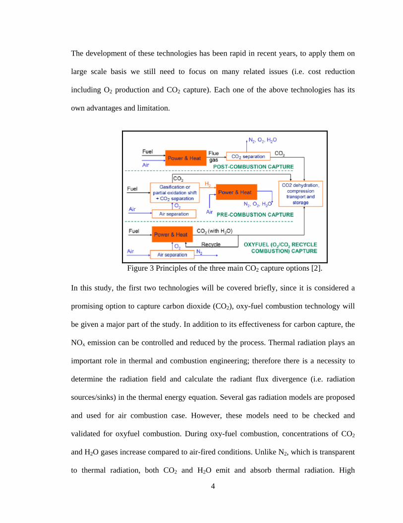
the need for carbon dioxide capture technology is increased. Nowadays, there are three

carbon capture technologies (CCS) are available (see Figure 3): 1) Post-combustion

capture technology, 2) Pre-combustion capture technology and 3) Oxy-fuel combustion

technology.

4

The development of these technologies has been rapid in recent years, to apply them on

large scale basis we still need to focus on many related issues (i.e. cost reduction

including O2 production and CO2 capture). Each one of the above technologies has its

own advantages and limitation.

Figure 3 Principles of the three main CO2 capture options [2].

In this study, the first two technologies will be covered briefly, since it is considered a

promising option to capture carbon dioxide (CO2), oxy-fuel combustion technology will

be given a major part of the study. In addition to its effectiveness for carbon capture, the

NOx emission can be controlled and reduced by the process. Thermal radiation plays an

important role in thermal and combustion engineering; therefore there is a necessity to

determine the radiation field and calculate the radiant flux divergence (i.e. radiation

sources/sinks) in the thermal energy equation. Several gas radiation models are proposed

and used for air combustion case. However, these models need to be checked and

validated for oxyfuel combustion. During oxy-fuel combustion, concentrations of CO2

and H2O gases increase compared to air-fired conditions. Unlike N2, which is transparent

to thermal radiation, both CO2 and H2O emit and absorb thermal radiation. High

5

concentrations of absorbing/emitting gases increase the emissivity of the flue gas with

subsequent effects on the radiative heat transfer.

1.2 PROBLEM STATEMENT

The influence of different gas radiation models on the results of air-fuel and oxyfuel

combustion is considered in this study. Results of the CFD modeling of a typical

industrial water tube boiler based on different gas radiation models are obtained and

evaluated. Fluent package software is utilized to simulate the combustion cases. The

study will focus on the following:

1. Discuss the importance of the oxy-fuel combustion as a promising technology to

lower greenhouse gases emission especially carbon dioxide CO2 and NOx.

2. Review a number of gas radiation models in terms of the range of applicability

and accuracy.

3. Simulate the combustion processes under air-fuel and oxyfuel environments with

different CO2/O2 ratios.

4. Make a grid independence survey of the findings by using three different grids.

5. Validation of the results should be warranted through the comparisons with the

experimental measurements.

6

1.3 OBJECTIVES

The objectives of the thesis are listed below:

1. Evaluating the influence of gas radiation models on the results of the CFD

modeling of air-fuel and oxyfuel combustion.

2. Analyzing the combustion performance of the typical industrial water tube boiler

under air-fuel and oxyfuel environments.

3. Investigating the effect of replacing N2 by CO2 on the combustion characteristics.

4. Determining the proper CO2/O2 ratio that would give the same temperature and

heat transfer characteristics as in the air-fuel combustion.

5. Checking the validity and accuracy of different gas radiation models for air-fuel

and oxyfuel combustion modeling.

6. Computing the error introduced in the results of oxyfuel combustion when the

weighted-sum-of-grey-gases model (WSGG), which developed by Smith for air-

fuel combustion, is used in the modeling.

7. Assessing the suitability of retrofitting the boiler to oxyfuel combustion.

7

1.4 THESIS OUTLINE

This thesis contains six chapters.

Chapter 1 introduces the subject of Carbon capture and Storage and importance of Oxy-

fuel combustion to mitigate greenhouse gases specially CO2. The problem statement and

objectives of the present thesis are discussed.

Chapter 2 is mainly a literature review and is divided in four sections. The first three

sections are about carbon capture technologies. The last section is the literature review on

oxyfuel combustion and gas radiation models.

Chapter 3 is an overview on the gas radiation models. It consists of nine sections; first

section is an introduction about gas radiation, second section is the derivation of the

radiative transfer equation, third section is about the solution methods of radiative

transfer equation, fourth section is the modeling of spectral nature of radiative transfer,

and finally the last five sections explain different gas radiation models.

Chapter 4 is the numerical solution of the combustion problem in the pilot scale furnace

under air-fuel and oxyfuel combustion conditions. The validation of radiation models

through comparison of the results with the measurements is presented. Chapter 5 is the CFD modeling of a typical industrial water tube boiler under air-fuel

and oxyfuel combustion. Grid independence of the boiler have been checked and

presented. Different gas radiation models have been evaluated and the characteristics of

air-fuel and oxyfuel combustions are compared.

Chapter 6 presents the conclusions of this study and some recommendation for future

work.

8

CHAPTER 2

CARBON CAPTURE TECHNOLOGIES

2.1 Post-Combustion Capture (PCC) Technology

In post-combustion capture method (see figure 4), a new final processing stage is applied

to remove most of the CO2 from the combustion products just before they are vented to

atmosphere. The most commercially advanced methods use wet scrubbing with aqueous

amine solutions. Amines-based solvents are suited to the lean combustion CO2

concentrations of flue gas (12–15 v/v% for coal and 4–8% for gas fired plants), but

require a large amount of energy to regenerate the solvent (in the solvent stripper), this

being as much as 80% of the total energy of the process. To compensate the energy used

in regeneration process, the additional fuel is required. CO2 is removed from the waste

gas by the amine solvent at relatively low temperatures (order 50 oC). The solvent is then

regenerated for re-use by heating (to around 120 oC), before being cooled and recycled

continuously. The CO2 removed from the solvent in the regeneration process is then

dried, compressed and transported to safe geological storage.

9

Figure 4 Post-combustion capture (PCC) process [3].

2.2 Pre-Combustion Capture Technology

In pre-combustion capture of CO2 (see figure 5), all types of fossil fuels can, however, be

gasified (partially combusted, or reformed) with sub-stoichiometric amounts of oxygen

(and usually some steam) at elevated pressures (typically 30–70 atmospheres) to give a

'synthesis gas' mixture of predominantly CO and H2. Additional water (steam) is then

added and the mixture is passed through a series of catalyst beds for the 'water–gas shift'

reaction to approach equilibrium: CO+H2O↔CO2+H2 (adding steam and reducing the

temperature promotes CO conversion to CO2). The CO2 can be separated to leave a

hydrogen-rich fuel gas. The separation process typically uses a physical solvent such as

pressure-swing-absorption, and methanol or polyethylene glycol (with commercial

brands called Rectisol and Selexol); CO2 is dissolved at higher pressure and then released

as the pressure is reduced. Because no heat is required to regenerate the solvent and the

CO2 can be released at above-atmospheric pressure, the energy requirements for CO2

capture and compression in pre-combustion capture systems may be of the order of half

10

that required post-combustion capture. But pre-combustion capture systems have to pay

an efficiency penalty for the shift reaction.

Figure 5 Pre-combustion capture process [3]

2.3 Oxy-Fuel Combustion Oxy-fuel or O2/CO2 recycle combustion is a relatively new Carbon Capture and

Storage (CCS) technology and is still at an early development stage compared to either

the post- or the pre-combustion CCS technologies. However, oxy-fuel technology

promises to be an economical alternative coupled with the possibility of higher CO2

capture rates. Oxy-fuel combustion is defined as the combustion of fossil fuels, in

nearly pure oxygen environment instead of air which is the conventional method

employed in steam power plants. Figure 6 illustrates power plant with oxy-fuel

technology. Specifically, 95% pure oxygen or higher is fed to the boiler via a cryogenic

distillation air separation unit. In addition to oxygen, the major part of the CO2-rich

11

exhaust flue gas is also recycled back to the boiler as a form of diluent, in order to

control combustion temperature. This is necessary, since combustion of coal in pure

oxygen gives a high flame temperature which will enhance the formation of NOx and

may cause damage to the boiler. Pulverized coal or other hydrocarbon fuel is then

combusted in this mixture of O2 and CO2 within the boiler.

Figure 6 Basic principle of oxyfuel technology [4].

2.4 Literature review

Radiative heat transfer is a prevailing phenomenon in many areas, devices and

equipment. That is especially the case if the temperatures are very high such as in a

combustion furnace. Radiative heat transfer characteristics of the flames, flue gases and

the particulate matter are very important to be considered in a boiler design. There is a

great necessity for mathematical models and computer codes that solve various radiation

problems. The real gases as carbon dioxide, water vapor and their mixtures are mainly

12

considered within these radiation problems. One of the important issues of the gas

radiation is the description of the radiative properties of real gases or of so-called non-

grey gases. The models used for defining the radiative properties of combustion gases in

radiation calculations can be roughly sorted in three groups [5]:

(1) Spectral line-by-line models,

(2) Spectral band models

(3) Global models.

The complexity of the models decreases from the line model to the global model. Each of

these models has its merits and drawbacks and consequently its area of application.

Historically, the oldest and the simplest concept for the prediction of radiation in gas is

grey gas model [6]. It assumes that the gas absorption coefficient is constant within entire

region of wavelengths. This model compared with others gives the predictions of very

poor accuracy [7]. The line-by-line (LBL) model provides the best accuracy. In this

method radiative transfer equation (RTE) is integrated over detailed molecular spectrum

for the gases. Because of the enormous amount of computational requirements, this

model is used only for benchmark solutions.

The statistical narrow band model (SNB) is very accurate in the prediction of radiative

transfer in high temperature gases. It gives the spectral transmissivity averaged over a

narrow band. Because of that, it is difficult to couple statistical narrow band model

(SNB) to the solution method of radiative transfer equation such as finite volume method

(FVM) where the values of spectral (monochromatic) absorption coefficient or its

average over a wavelength interval is needed. Also the disadvantage of statistical narrow

band model (SNB) is that it requires a large number of bands, and therefore is very

13

expensive for computation. Wide band model (WBM) is a simplification of the statistical

narrow band model (SNB). Instead of spectral lines, it works with bands and is more

economical. Wide band model (WBM) is less, but still reasonable accurate. It yields wide

band absorptance while the solution of radiative transfer equation (RTE) by finite volume

method (FVM) operates either with spectral or with averaged absorption coefficient.

Therefore Wide band model (WBM) cannot easily and simply be incorporated in finite

volume method (FVM). In addition, the Wide band model (WBM) requires the

knowledge of the path length in the model as well as the spectral parameters associated

with this path length.

Line-by-line models (LBL), statistical narrow band model (SNB) and Wide band model

(WBM) are very accurate gas radiative properties models, but they require enormous

amounts of computer time. This is undesirable even nowadays when powerful

supercomputers are available since a gas radiative properties model is only a part of a

radiation calculation. A radiation calculation is in turn only a part of a complex

computational fluid dynamics (CFD) code that describes fire and combustion comprises

3-D turbulent multiphase fluid flow, chemical reactions and heat transfer by radiation,

convection and conduction.

The global gas radiative properties models such as those of Hottel and Sarofim’s [6],

Steward and Kocaefe’s [8, 9] and Smith et al.’s [10] are based on the concept of

weighted sum of grey gases model (WSGG). The weighted sum of grey gases model

(WSGG) was first established by Hottel and Sarofim [6]. It replaces the radiative

properties of real gases or of non-grey gases with an equivalent finite number of grey

gases. The weighted sum of grey gases model (WSGG) is used for evaluation of total gas

14

emissivity and total gas absorptivity for a given path length. For each of the grey gases,

the absorption coefficient taken as temperature independent, and the weighting factors

taken as temperature dependent in polynomial form, should be evaluated. Even weighted

sum of grey gases model (WSGG) is established for the evaluation of gas emissivity and

absorptivity, when weighted sum of grey gases model (WSGG) is coupled with the

solution of radiative transfer equation (RTE) only absorption coefficients and weighting

factors of grey gases are used and never the total gas radiative properties.

The radiative transfer were calculated in 2-D, i.e. in axisymmetric cylindrical enclosures

[11, 12] by using statistical narrow band model (SNB) with a ray tracing method. Also

the statistical narrow band model (SNB) combined with a ray tracing method was used in

axisymmetric cylindrical enclosure in [13]. The predictions based on the ray tracing

method are extremely expensive and cannot be used to standard engineering calculations

due to difficulties related to the linking of the radiative transfer equation (RTE) with

narrow band model (SNB) and Wide band model (WBM).

Modest has shown [14] that weighted sum of grey gases model (WSGG) can be

generalized for use with any arbitrary solution method of radiative transfer equation

(RTE). This method needs evaluation of the grey gas weighting factors and absorption

coefficients (for each grey gas) for any used gas species or their mixtures. The Spectral

line weighted sum of grey gases model (SLW) [15, 16] appeared as a more accurate

version of weighted sum of grey gases model (WSGG). Within the Spectral line

weighted sum of grey gases model (SLW) the weights of classical weighted sum of grey

gases model (WSGG) were evaluated by using the absorption-line black-body

distribution function. This function is calculated directly from the high-resolution

15

molecular spectrum of gases. Instead of integration of radiative transfer equation (RTE)

over wavenumber, now the quadrature is carried out over absorption cross section. Very

similar to the Spectral line weighted sum of grey gases model (SLW) is the absorption

distribution function (ADF) concept [17, 18]. It differs from the Spectral line weighted

sum of grey gases model (SLW) only how the weighting factors are calculated. The

weighting factors are evaluated in such a way that emission of an isothermal gas is

strictly calculated for actual spectra.

Trivic [19] has developed a 3-D mathematical model for predicting turbulent flow with

combustion and radiative heat transfer within a furnace. The model consists of two

sections:

(1) Transport equations that are non-linear partial differential equations solved by

a finite difference scheme.

(2) The radiative heat transfer that was analyzed by the zonal method.

The link between these two sections is a source-sink term in the energy equation. The

radiative properties of combustion gases were represented by two different models:

(1) Hottel and Sarofim’s model and,

(2) Steward’s model.

The Monte Carlo method was used to evaluate total radiative interchange in the system

between zones. The Mie equations were used for the determination of the radiative

properties of particles suspended in the combustion gases. The mathematical model was

validated against experimental data collected on two large furnaces:

(1) A tangentially pulverized coal fired boiler of 220 MW

16

(2) An oil fired boiler of 345 MW, with symmetrically positioned burners at the

front and rear wall.

The tests and calculations were performed for several loads for both boilers. The

measured and predicted gas temperature and heat flux distributions within the boilers

were compared. The results gave reasonable agreement between measurements and

values predicted by the model.

Coelho [20] has carried out 3-D numerical simulations of radiative heat transfer from

non-grey gases by the discrete ordinate method (DO) and the discrete transfer method

(DTM). He has used several gas radiative properties models as CK model, the Spectral

line weighted sum of grey gases model (SLW) and weighted sum of grey gases model

(WSGG). The predictions were compared against the ray tracing statistical narrow band

model (SNB) results [21] that were used as benchmark data. Coelho has concluded, inter

alia, the following:

(1) The weighted sum of grey gases model (WSGG) is computationally

economical and has moderate accuracy.

(2) The Spectral line weighted sum of grey gases model (SLW) is a compromise

between accuracy and numerical requirements but it needs additional work for an

optimization of the coefficients.

(3) The CK model is the most accurate but too time consuming for engineering

applications.

The comparison of the predictions calculated by nine total emissivity models against the

calculations done by exponential wide band model (EWBM) was carried out [7]. One of

17

the main conclusions was that Smith et al. weighted sum of grey gases model [10]

indicates the advantage.

Trivic [22] has developed a new 3-D non-grey gas mathematical model and computer

code for radiation, based on the coupling of finite volume method (FVM) and weighted

sum of grey gases model (WSGG) convenient for incorporation within CFD codes. Since

it is showing the advantage compared with others, Smith et al.’s weighted sum of grey

gases model (WSGG) was incorporated in this model.

During oxy-fuel combustion, concentrations of CO2 and H2O gases increase compared to

air-fired conditions. Unlike N2, which is transparent to thermal radiation, both CO2 and

H2O emit and absorb thermal radiation. High concentrations of absorbing/emitting gases

increase the emissivity of the flue gas with subsequent effects on the radiative heat

transfer.

Buhre et al [23] have reviewed the status and the research needed for oxy-fuel

technology. The understanding of oxy-fuel combustion has been established primarily

from pilot-scale studies, as it has not been applied at practical scale, and there have been

few fundamental studies. Buhre stated that the oxy-fuel combustion and CO2 capture

from flue gases is a near-zero emission technology that can be adapted to both new and

existing pulverized coal-fired power stations. In the oxy-fuel technology the

concentration of carbon dioxide in the flue gas is increased from approximately 17 to

70% by mass. The carbon dioxide can then be captured by cooling and compression for

subsequent transportation and storage.

Wall [3] has stated that the heat transfer prediction are critical for oxy-fuel technology,

since there are changes in gas properties due to CO2 recycling from outlet back to the

18

furnace inlet. These changes are attributed to alteration of gas radiative properties and

gas heat capacity. During oxy-fuel combustion, the flue gas tri-atomic molecules

concentration increases drastically and this will lead to change in the gas emissivity.

Hottel et al [6] showed that the major contributor of heat transfer from a flame from

conventional fuels is thermal radiation from water vapor, carbon dioxide, fly ash, soot

and carbon monoxide. Any change of CO2 and H2O concentrations yield to change in

radiative heat transfer. For air combustion with conventional partial pressures of CO2 and

H2O, the heat transfer calculation carried out by using a 3 grey-one clear gas model to

estimate flame emissivity. In oxy-fuel combustion the 3 grey-one clear gas model should

be validated and/or modified or replaced by a more accurate model [6, 24], carbon

dioxide and water vapor also have high thermal heat capacities compared to nitrogen.

Kumar et al [25] have conducted some measurements on coal devolatilisation, they

concluded that devolatilisation in an atmosphere of O2/CO2 is greater than in O2/N2 due

to char gasification by CO2. The elevated CO2 concentration surrounding the burning

char particles could also result in gasification reactions contributing to the char mass loss.

Measurements by Kumar et al [25] indicate that coal and char reactivity can differ at the

same O2 levels in O2/N2 and O2/CO2 environments. Even if the reactivities in the two

environments are identical, coal burnout will improve in an oxy-fuel retrofit due to:

The higher O2 partial pressures experienced by the burning fuel,

Possible gasification by CO2

Longer residence times due to the lower gas volumetric flows.

19

Haynes et al [26] discussed the influence of gaseous additives on the formation of soot in

diffusion flames. They concluded that addition of CO2 and H2O to the oxidizer, as well

as replacement of N2 by CO2 in the oxidizer, will reduce soot formation in the flame.

Shaddix et al [27] found that gasification reaction of the char by CO2 becomes significant

under oxygen-enriched char combustion at temperatures prevailing in practical processes.

Gaseous pollutant formation and emissions are changing during oxy-fuel combustion, as

a result of sulfur retention in ash and deposits; the SOx emissions per energy of fuel

combusted may be lowered by less than 20%, depending on ash composition and NOx

emissions generated per unit of energy are reduced by up to 70% [3]. Kimura et al [28]

stated that during oxy-fuel combustion, the amount of NOx exhausted from the system

can be reduced to less than one-third of that with combustion in air.

According to Okazaki et al [29] the mechanisms lead to NOx reduction are:

• Decrease of thermal NOx due to the very low concentration of N2 from

air in the combustor.

• The reduction of recycled NOx as it is reburnt in the volatile matter

release region of the flame.

• The reaction between recycled NOx and char.

They concluded by experiments that the reduction of recycled NOx is the dominant

mechanism for the reduction in NOx emissions. They estimated that more than 50% of

the recycled NOx was reduced when 80% of the flue is recycled.

20

Croiset et al [30, 31] noted that the conversion of coal sulphur to SO2 decreased from

91% for the air case to about 64% during oxy-fuel combustion. In the oxy-fuel

combustion, SO2 concentration is higher than that from air combustion due to flue gas

recirculation.

Molburg et al [32] stated that there is a need for desulphurization of the recycled flue gas

for oxy-fuel combustion to reduce corrosion impact on the furnace.

Khare et al [33] noted that in order to achieve the same O2 fraction in the flue gas as in

air firing, the excess O2 from 3% to 5% for dry and wet recycle is required for oxy-fuel

combustion. Also, oxygen concentrations at the burner inlet range from 25% to 38%

(v/v) to achieve matched furnace heat transfer depending on the use of dry or wet recycle

with some impact of furnace size. Changes to the plant or its operation may be required

to maintain design output by achieving a satisfactory balance for heat transfer in the

different sections of the furnace. The balancing of heat transfer appears to depend on the

extent of drying of the recycle stream [34].

Preliminary heat transfer calculations for retrofitted boiler have also been performed by

the University of Newcastle [35]. The calculations revealed that retrofitting of existing

boilers with oxy-fuel technology results in different heat transfer impacts. For the same

adiabatic flame temperature, furnace heat transfer increases and convective pass transfer

decreases. As the furnace heat transfer is dependent on the furnace size, the impact is

scale (i.e. boiler size) dependent.

A study has been done by Payne et al. [36] including experiments in a 3 MW test

furnace; they investigated the efficiency of the recycle rate as a tuning parameter with the

purpose of establishing similar heat transfer characteristics in oxy-fuel as in air-firing in

21

retrofits of existing boilers. In addition, a modeling study of a 50 MW furnace has been

conducted in the same work; the results showed that similar overall heat transfer

(radiative + convective) could be established during both dry and wet recycling of flue

gases at certain recycle rates and to get the same adiabatic flame temperature as for air

case the oxygen concentrations should be lower than 30%. Finally, they concluded that

the recycle rate is an appropriate tuning parameter to achieve similar boiler performance

for air and oxy-fuel combustion.

CFD models for oxy-fuel combustion have been published for flame models by Chui and

Tan [37] to predict NOx formed in a pilot-scale furnace.

Tan et al. [38] performed natural-gas-fired oxy-fuel experiments in a 300 kW refractory

lined combustor. Total heat flux measurements showed that an oxy-fuel flame with 28%

vol oxygen and an air flame produced similar total heat flux profiles. The temperature

conditions were almost identical for air and oxy-fuel conditions. Zheng et al [39, 40]

modeled the heat transfer in a boiler to assess the suitability of retrofitting an air-fired

boiler to oxy-fuel combustion. The gas emissivity was calculated from the correlations

for total gas emissivity for the water vapor and carbon dioxide suggested by Leckner

[41]. The studies indicated that the lower and upper part of an air-fired boiler can be

made to perform properly without major modification when converting from air firing to

oxy-fuel combustion.

Andersson and Johnsson [42] have studied experimentally the combustion of propane

fuel for 3 test cases: air-combustion (referenced one) and other two oxy-combustion

cases (OF21 @ 21% O2 and OF27 @ 27% O2). The difference in total radiation intensity

between these cases is determined and compared. The mean emissivity is then

22

determined based on the experimental data and as a comparison the gas emissivity is

calculated by an existing gas emissivity model given by Leckner [41]. In addition the

difference in combustion environment is described. One of the results they have reported

is in case of the OF 21combustion, the temperature levels were lower compared to air-

fired condition and this is returned to two reasons; 1) the higher specific heat capacity of

CO2 compared to N2, and 2) increase in radiation losses caused by the CO2 with increase

the gas emissivity. In addition, the physical volume of the high temperature zone of

OF21 case is smaller compared to the two other cases. The gas composition of the flame

envelope is clearly different from the rest; the amount of unburned hydrocarbons is

significantly higher. In spite of the lower temperature levels of the OF21 case compared

to the air case, the OF21 radiation intensities are approximately similar to those of air

case. Furthermore, the temperature levels in the OF27 combustion approach those of the

air case and the radiation intensity is higher than that in the air case despite the fact that

the temperature levels are lower or similar to those of air. It is also found that, the flame

radiation intensity increases with up to 30% and the incident wall intensity by 20%

compared to air fired conditions. Finally, they concluded that the difference between

oxyfuel combustion and air combustion can be partly explained by the high CO2 content

in the combustion gases, i.e.CO2 partial pressure approximately eight times the pressure

level of normal air-fired condition, and the increase in the total emissivity of oxyfuel

combustion flame is attributed to the increased emissivity of the CO2. In general, changes

in soot volume, CO2 and H2O concentration levels are very important factors in modeling

the radiative heat transfer for O2/CO2 flames.

23

In the most recent study, Johnsson et al [43] have evaluated several approximate gas

radiative property models for oxy-fuel environments in large atmospheric boiler. These

models were Statistical narrow band (SNB) models, weighted-sum-of-grey-gases model

(WSGG), spectral line-based weighted-sum-of-grey-gases model (SLW) and two grey-

gas approximations model. The parameters of statistical narrow band models (SNB) are

taken from three sets of databases:

1) Leckner [41, 44]

2) Grosshandler (RADCAL) [45]

3) Taine et al [46, 47, 48] at EM2C lab

The model uses the last database is considered the benchmark model which all other

model are compared to. The weighted-sum-of-grey-gases model (WSGG) coefficients

have been fitted to emissivities calculated with the EM2C SNB model in the temperature

range of 500-2500 K and path lengths between 0.01 and 60 m and atmospheric pressure.

The two grey models; one is based on weighted-sum-of-grey-gases model WSGG (4+1)

and the other based on EM2C SNB model are tested.

The accuracy of the models is investigated in a number of cases; (uniform and non-

uniform) and (wet and dry flue gas) both in terms of intensity of single path, radiative

source term and wall flux for a domain between two infinite plates. Temperature and gas

concentration profiles used in the investigation for non-isothermal paths are based on

experiments conducted in a test furnace, where air and O2/CO2 combustion of a propane

flame were studied [49]. The O2 concentration in the feed gas for an oxy-fuel flame was

27% and the recycle flue gas was dry, given a mole fraction of CO2 around 0.8 in the

24

furnace. Radial profiles of gas temperature and concentration of O2, CO and CO2 and

total hydrocarbons were measured at different heights in the furnace. The radiation

intensity was recorded with a narrow angle radiometer. It is noted that, for the total

intensity of the uniform paths, the discrepancies between the statistical narrow band

models (SNB) are below 5%. The Spectral line weighted sum of grey gases model

(SLW) and weighted sum of grey gases model (WSGG) (3+1) are in a good agreement

with the benchmark model deviating less than 10%. The grey model gives a different

shape of the intensity profile, although the intensity at the end of the path is correct. For

the total intensity of the non-uniform paths, it is found that, the difference between the

statistical narrow band models (SNB) is as high as 25% at the end of the path in the case

of wet flue gas and within 10% during dry flue gas. The maximum discrepancy of

weighted sum of grey gases model (WSGG) (3+1) is 15% but less than 10% in most

regions and the deviation between the spectral line-based weighted-sum-of-grey-gases

model (SLW) and the EM2C statistical narrow band model (SNB) is 5-10%. The grey

models give both an incorrect shape of the profile and a significant error at the end of the

path. The comparison of the incident wall flux between the models is carried out in the

study, it is shown that the difference between the statistical narrow band models (SNB) is

30% at the longest path in the wet flue gases case whereas 15% for dry flue gases. The

weighted sum of grey gases model (WSGG) (4+1) deviates less than 20 % at recycling of

wet flue gas and less than 10% at dry flue gas recycling. The spectral line-based

weighted-sum-of-grey-gases model (SLW) with its larger number of gases agrees very

well with the EM2C statistical narrow band model (SNB). Finally, in term of radiative

source quantity, the difference between the statistical narrow band model (SNB) is about

25

5-20%. The deviation of the weighted-sum-of-grey-gases model (WSGG) models is with

a few exceptions less than 20%.

The accuracy of the radiation models is determined by the importance of the radiative

source term. Lallemant et al [7] pointed out that in regions of intensive combustion, the

heat released by combustion dominates over the radiative release, and the energy radiated

away from non-luminous flames hardly exceeds 10-15% of the total heat release in the

flame. In addition, they compared gas radiation models with measurements of total

radiation intensity in a 300 kW non-sooting natural-gas flame. The agreement between

measurements and computed exponential wide band model (EWBM) data is excellent for

measurements against cold furnace walls.

Habib et al [50] have compared the characteristics of oxyfuel combustion to those of air–

fuel combustion in a typical natural gas fired package boiler. The percentages of recycled

CO2 considered in their study were 83.8% and 77% by mass. The first corresponds to

21% O2 and the second corresponds to 29% O2 by volume. Results indicated that the

temperature levels are reduced in oxyfuel combustion. As the percentage of recirculated

CO2 is increased, the temperature levels are greatly reduced. They found that the fuel and

oxygen consumption rates are slower in oxyfuel combustion relative to air–fuel

combustion. Furthermore, heat transfer from the burnt gases to the water jacket along the

different surfaces of the furnace was calculated. It is shown that the energy absorbed is

much higher in the case of air–fuel combustion along all surfaces except for the end part

of the furnace close to the furnace rear wall. The heat transfer in the return chamber (tube

bank) was also calculated and the results indicated higher heat transfer in the oxyfuel

26

case in comparison with the air fuel case as a result of ignition delay in the vicinity of the

furnace entrance region.

The weighted sum of grey gases model (WSGG) is recommended for CFD applications

when the radiative source term has a significant influence and reasonable estimates of

wall fluxes are required. The drawback of the model is the need for specific sets of

coefficients at different H2O/CO2 ratios and most of the available coefficients are fitted

to air-fired conditions.

Porter et al [51] have used the spherical harmonic (P1) and the discrete ordinates method

(DO) to solve the radiative transfer equation (RTE) in multi-dimensional problem. The

spectral nature of radiation has been treated by using non-grey gas full spectrum k-

distribution method (FSCK) and a grey method. The simulation results of air-fuel and

oxyfuel combustion are compared with the statistical narrow band model (SNB). They

concluded that the non-grey full spectrum k- distribution method was in good agreement

with the statistical narrow band model (SNB). Significant errors are introduced in the

wall heat flux when a grey model is used. In addition, using the smith grey weighted

sum of grey gases model (WSGG) leads to substantial errors in the radiation source

calculation which changes the predicted temperature.

Weighted sum of grey gases model (WSGG), which was developed by Smith [10], is

fitted for air-fuel combustion. This model was modified by Johansson et al [52] to be

suitable to cover the temperature range of 500–2500 K, pressure path lengths of 0.01–60

bar m and molar ratios of H2O and CO2 between 0.125 and 2. This range of molar ratios

covers both oxy-fuel combustion of coal, with dry- or wet flue gas recycling, as well as

27

combustion of natural gas. They have reported that the modified weighted sum of grey

gases model (WSGG) is a computationally efficient option for CFD simulations.

Hjärtstam et al [53] have utilized the CFD method to investigate the influence of gas and

gas-soot radiation mechanisms in air and oxyfuel flames when Propane fuel is burnt in a

100 kW test furnace. In their study, a grey model was examined in order to know if it is

sufficient to generate a reliable solution when applied in CFD simulation of oxyfuel

combustion. They have shown that in the case of Oxyfuel combustion both grey and non-

grey weighted sum of grey gases models (WSGG) overestimate the peak temperature,

however, the results of non-grey model are closer to the measurements than that of grey

model. In addition, they stated that the inclusion of soot modeling in both grey and non-

grey gas radiation models has a significant impact in the CFD calculations.

28

CHAPTER 3

GAS RADIATION MODELS

3.1 Introduction

Thermal radiation plays an important role in thermal and combustion engineering. This is

especially true for applications involving high-temperature chemically reacting flows

where radiation can dominate the total energy transfer in the system. A combustion

device is a concrete example where one typically needs to calculate the flame structure

and heat transfer in the system in multiple dimensions systems. For such a purpose one

must determine the radiation field and calculate the radiant flux divergence (i.e. radiation

sources/sinks) in the thermal energy equation [54]. The calculation of the radiant energy

quantities is coupled to the transport equations for the momentum, energy and species

concentration distributions. Nowadays engineers are confronted with complex

combustion phenomena that depend on interrelated processes of thermodynamics,

chemical kinetics, fluid mechanics, heat and mass transfer, turbulence and radiative

transfer. Computational fluid dynamics (CFD) tools are needed to help understand,

design, optimize and operate high-temperature combustion devices where radiative

transfer is an important mode of energy transport. Owing to the nature of the radiative

transfer equation (RTE) such CFD computations are very time-consuming, because there

is a need to integrate the radiation field (intensity) over all directions and the entire

29

spectrum [19]. Research efforts have been under way for the past several decades to

make the computations more efficient and cost effective so that computational fluid

dynamics tools could be used to perform design and optimization calculations. During

the last several decades, considerable progress has been made in predicting radiative

transfer in multidimensional “enclosures” containing absorbing, emitting and scattering

media such as mixtures of gases and gases/polydisperse particles [58]. Because the

radiative transfer equation (RTE) is similar to the equations used for simulating neutron

transport and flow of rarified gases, researchers have often adopted and assimilated the

methods developed by scientists in these fields to solve radiation heat transfer problems

encountered in thermal/combustion systems [56]. When calculating radiation heat

transfer in a combustion device, probably the first and most important decision one has to

make is about the choice of the radiative transfer model, which is dictated by the specific

application and the level of detail needed to analyze the problem. For example, the level

of detail required to determine the local temperature and species concentration

distributions in a flame is much greater than that required to calculate the local radiant

heat flux on a load in a furnace or on the furnace wall. Next, one must decide if detailed

spectral calculations of radiation transport is warranted or some approximate band model

or grey treatment of radiative transfer will be adequate. One must also choose a

numerical method for solving the radiative transfer equation (RTE) that is compatible

with the technique employed for solving the transport equations. Finally, the model

should also be accurate, robust and predict the desired radiant energy quantities in a

computationally efficient manner [54].

30

The accuracy of radiative transfer predictions in combustion systems cannot be better

than the accuracy of the radiative properties of the combustion products used in the

analysis. These products usually consist of combustion gases such as water vapor, carbon

dioxide, carbon monoxide, sulfur dioxide, and nitrous oxide, and particles, like soot, fly-

ash, pulverized-coal, char or fuel droplets. Before attempting to tackle radiation heat

transfer in practical combustion systems, it is necessary to know the radiative properties

of the combustion products. Considering the diversity of the products and the probability

of having all or some of these in any volume element of the system, it can easily be

perceived that the prediction of radiative properties in combustion systems is not an easy

task. The wavelength dependence of these properties and uncertainties about the volume

fractions and size and shape distribution of particles cause additional complications [6].

3.2 Radiative Transfer Equation (RTE)

Two theories have been developed for the study of the propagation and interaction of

electromagnetic radiation with matter, namely, the classical electromagnetic wave theory

and the radiative transfer theory. The theories were developed independently and there is

no similarity in their basic formulations. Conceptually, they are completely distinct;

however, both theories describe the same physical phenomenon. The classical

electromagnetic theory has approached the study of propagation and interaction of matter

with radiation from the microscopic point of view and the radiative transfer theory from

the macroscopic (or phenomenological) point of view. The study of the detailed

interaction between electromagnetic radiation and matter on the microscopic level from

both the classical and quantum mechanics point of view yields the interaction cross-

31

sections of the particles making up the matter [57]. This fundamental approach predicts

the macroscopic properties of the media, and these properties appear as coefficients in

the radiative transfer equation. The quantitative study, on the phenomenological level, of

the interaction of radiation with matter that absorbs, emits, and scatters radiant energy is

the concern of the radiative transfer theory. The theory ignores the wave nature of

radiation and visualizes it in terms of light rays of photons. These are concepts of

geometrical optics. The geometrical optics theory is the study of electromagnetism in the

limiting case of extremely small wavelengths or of high frequency. The detailed

mechanism of the interaction process involving atoms or molecules and the radiation

field is not considered. Only the macroscopic problem consisting of the transformation

suffered by the field of radiation passing through a medium is examined. Thus, there is a

considerable simplification over the electromagnetic wave theory. The radiative transfer

equation (RTE) forms the basis for quantitative study of the transfer of radiant energy in

a participating medium [24]. The equation is a mathematical statement of the

conservation principle applied to a monochromatic pencil (bundle) of radiation and can

be derived from many viewpoints. The RTE is based on application of an energy balance

on an elementary volume taken along the direction of a pencil of rays and confined

within an elementary solid angle. The detailed mechanism of the interaction processes

involving particles and the field of radiation is not considered here. On the

phenomenological level only the transformation suffered by the radiation field passing

through a participating medium is examined. The derivation accounts mathematically for

the rate of change of radiation intensity along the path in terms of physical processes of

absorption, emission, and scattering.

32

Consider a cylindrical volume element, figure 7, of cross-section dA and length ds in an

absorbing, emitting, and scattering medium characterized by the spectral absorption

coefficient ĸv , scattering coefficient σv [54]. The axis of the cylinder is in the direction of

the unit vector →

S , i.e. ds is measured along →

S . The spectral intensity of radiation (spectral

radiance) in the →

S -direction incident normally on one end of the cylinder is Iv and the

intensity of radiation emerging, through the second end in the same direction is Iv + dIv.

Here, v is the frequency and is related to the wavelength λ by v = c / λ, where c is the

speed of electromagnetic wave in vacuum.

Figure 7 coordinates for derivation of the radiative transfer equation [54].

It follows from the definition of the spectral intensity Iv that radiant energy incident

normally on the infinitesimally small cross-section dA during time interval dt, in

frequency range dv and within the elementary solid angle dΩ about the direction of the

unit vector →

S is

Iv dA dΩ dv dt (1)

The emerging radiant energy at the other face of the cylinder in the same direction equals

(Iv + dIv ) dA dΩ dv dt (2)

33

The net gain of radiant energy, i.e. the difference between energy crossing the two faces

of the cylinder, is then given by

(Iv + dIv - Iv ) dA dΩ dv dt = dIv dA dΩ dv dt (3)

The loss of energy from this pencil of rays due to absorption and scattering in the

cylinder is

(ĸv + σv) Iv ds dA dΩ dv dt (4)

The emission by the matter inside the cylindrical volume element dV, in the time interval

dt, in the frequency range dv confined in the solid angle dΩ about the direction →S equals

ĸv n2v Ibv dV dΩ dv dt (5)

Where Ibv is Planck's spectral blackbody intensity of radiation, and nv is the spectral

index of refraction of the medium. The increase in energy of the pencil of rays (→

S , dΩ)

due to in-scattering of radiation by the matter into the elementary cylindrical volume

from all possible directions →S is

dtddAdddsIssds v ννννπ

σν π

νν ΩΩ×→→Φ∫ ∫∆ =Ω

])();(41[ ''

4

'''

' '

'

(6)

In this expression the phase function Φv(→

S ' → →

S ; v'→v) dΩ'dv' / 4π represents the

probability that radiation of frequency v' propagating in the direction →

'S and confined

within the solid angle dΩ' is scattered through the angle ( →

S , →S ) into the solid angle dΩ

and the frequency interval dv. This probability is determined by the scattering

mechanism. For coherent scattering the phase function is independent of frequency v' and

reduces to Φv(→

S' → →S ).

Since in this case the sum of probability over all directions must equal unity, we must

have

34

1)(41)(

41)(

41

44

''

4

'

'

=ΩΨΦ=Ω→Φ=Ω→Φ ∫∫∫=Ω=Ω=Ω

ddssdssπ

νπ

νπ

ν πππ

(7)

This implies that for coherent scattering the spectral phase function is normalized to

unity. The scattering angle Ψ, i.e. the angle between →S ' and →S can be expressed as

cos Ψ= cos θ cos θ ' + sin θ sin θ 'cos(ϕ - ϕ ') (8)

Or

cos Ψ = ξ ξ '+ ηη' + μμ' (9)

Where

ξ = sin θ cos ϕ, η = sin θ sin ϕ, μ = cosθ (10)

are the direction cosines in any orthogonal coordinate system. Reference to figure 1, →

S'

(θ ', ϕ') represents the incoming direction of the pencil of rays, and →

S (θ, ϕ), is the

direction of the pencil after scattering.

Equating the change of energy in the cylindrical volume element to the net gain or loss of

energy along the traversal path of the cylinder in terms of the processes of attenuation,

emission and in-scattering yields [57]

dIv dA dΩ dv dt = -(ĸv + σv) Iv ds dA dΩ dv dt + ĸv n2v Ibv dV dΩ dv dt +

dtddAdddsIssds v ννννπ

σν π

νν ΩΩ×→→Φ∫ ∫∆ =Ω

])();(41[ ''

4

'''

' '

'

(11)

Dividing this equation by ds dA dΩ dv dt and recalling that the distance ds traversed by

the pencil of rays is cdt, where c is the velocity of light in the medium, yields the

equation of transfer in a Lagrangian coordinate system

''

4

'''2

' '

' )();(4

)(1 νννπσ

κσκν π

νν ddsIssInI

dtdI

c vbvvvvvvv Ω→→Φ+++−= ∫ ∫

∆ =Ω

(12)

35

Clearly, the left-hand side of this integro-differential equation represents the net change

in Iv per unit length along the path ds = c dt. Equation (12) is a statement of the

conservation of energy principle for a monochromatic pencil of radiation (in the

direction →

S ) and is generally called the "radiative transfer equation" (RTE) [57].

The substantial derivative d/dt refers to the rate of change of spectral intensity as seen by

an observer propagating along with the velocity of radiation (Lagrangian coordinates). In

terms of a coordinate system fixed in space (Eulerian coordinates), radiative transfer

equation (RTE) may be written as

)()(11vvvv

vv ISIstI

cdtdI

c−=⋅∇+

∂∂

= β (13)

where the source function Sv represents the sum of emitted and in scattered radiation and

is defined as radiant energy leaving an element of volume of matter in the direction

( →

S ,dΩ) per unit volume, per unit solid angle, per unit frequency, and per unit time,

''

4

'''2

' '

' )();()4/1)(/()/( νννπβσβκν π

νν ddsIssInS vvvbvvvv Ω→→Φ×+= ∫ ∫∆ =Ω

(14)

In general the intensity is a function of three spatial coordinates, two angles and time; of

course, the seventh independent variable required to define the radiation intensity is the

wavelength or the frequency of radiation.

The radiative transfer equation (12) is an integro- differential equation, and because of

this it is very difficult to solve exactly for multidimensional geometries. Therefore, some

simplifications of this equation are necessary. A close look at the source term given in

equation (14) reveals that the in-scattering term (the second term of the right hand side)

yields the integral nature of the radiative transfer equation (RTE). If scattering is

negligible in the medium, then the equation (14) will be a differential equation, which is

36

much easier to solve than the integro-differential equation. Calculation of radiative

transfer requires two types of models [58]:

(1) Models to account for directional nature of radiation; and

(2) Models to describe the spectral nature of radiation.

Since, the directional and spectral models are not coupled or directly related, they can be

discussed separately. Numerous approaches for both types of models have been

proposed, and they will be divided into several groups for more logical and coherent

discussion.

3.3 Radiative Transfer Equation (RTE) Solution Methods

3.3.1 Introduction The radiative transfer equation is an integro-differential equation, and its solution even

for a one dimensional, planar, grey medium is quite difficult. Most engineering systems,

on the other hand, are multidimensional. In addition, spectral variation of the radiative

properties must be accounted for in the solution of the radiative transfer equation (RTE)

for accurate prediction of radiation heat transfer. These considerations make the problem

even more complicated [54]. Therefore, it is almost necessary to introduce some

simplifying assumptions for each application before attempting to solve the radiative

transfer equation (RTE) in its general form. It is not possible to develop a single general

solution method for the equation which would be equally applicable to different systems.

Consequently, several different solution methods have been developed over the years.

37

According to the nature of the physical system, characteristics of the medium, the degree

of accuracy required, and the available computer facilities, one of several different

methods can be adopted for the solution of the problem considered. Before choosing one

solution method over another, it is important to know the advantages and disadvantages

of each method. In this section, several radiative transfer models of interest to

combustion systems and their features will be discussed. 3.3.2 Overview of computational methods in radiative transfer During the last four decades numerous methods have been developed. These methods for

calculating radiative transfer in multidimensional geometries can be grouped into four

broad categories [58];

(1) Directional averaging approximations;

(2) Differential approximations (moment, modified moment, spherical harmonics,

etc.);

(3) Energy balance (zone, Monte Carlo, finite volume, finite element, boundary

element, etc.) methods; and

(4) Hybrid (discrete transfer, zone-Monte Carlo, ray tracing, etc.) methods.

The asymptotically thin and thick approximations are simple but unfortunately their

ranges of validity are very limited; therefore, only the general optically self- absorbing

situations are considered here. All of the directional averaging approximations involve

some type of averaging of the radiance field with direction. The two-, four-, six-, and

multi-flux methods (MFM) are probably the simplest to apply. The shortcomings of

MFMs are primarily twofold [58]. First, the accuracy of the predictions depends on the

38

arbitrary choice of the solid angle subdivision over which the intensities are integrated to

obtain the fluxes. Second, the fluxes for one direction are not coupled with those of

another direction if the medium is not scattering.

The first order differential approximations of the radiative transfer equation (RTE)

(moment and spherical harmonics) are capable of treating radiatively participating media

with scattering. They yield radiative transfer predictions of reasonable accuracy and can

be adopted for band calculations. The discrete ordinates method (DO) for approximating

the radiative transfer equation (RTE) and the finite volume method (FVM) for solving

the radiative transfer equation (RTE) numerically are compatible with CFD methods for

solving transport problems in combustion systems.

Energy balance methods such as the zone method (ZM) and its extensions as well as the

boundary element method (BEM), which can be considered as a variant of the zone

method (ZM), require exceedingly large storage for the local exchange factors if the

methods are to be used to calculate the local quantities. The method is suitable for

calculating heat fluxes or global heat transfer rates in a furnace if the temperatures and

radiating species concentrations are known. The disadvantage of the zone method (ZM)

and boundary element method (BEM) solvers is the difficulty of generating fine meshes

in regions of large temperature and species concentration gradients (i.e. flame structure)

as well as the difficulty in evaluating integrals whose integrands are singular. The

statistical Monte Carlo method (MCM) is incompatible with CFD procedures for solving

the transport equations.

The discrete transfer method (DTM) is considered a hybrid method because it is derived

from the combination of flux methods and the Monte Carlo method (MCM) for choosing

39

the finite number of directions of the radiative transfer equation (RTE). The method is

well suited for CFD calculations. The disadvantages of the other hybrid methods are the

same as those of the energy balance methods.

3.3.3 Discrete Ordinate Method (DO) The discrete ordinates method (DO) is also in a way a multi-flux method (MFM), but is

considered separately because of its importance. The method does not require any

assumptions concerning the directional dependence of the intensity. It was originally

suggested by Chandrasekhar [59] for astrophysical applications, and detailed derivation

of the relevant model equations were discussed in application to neutron transport

problems. The method has been applied to solve radiation heat transfer problems

including those arising in combustion systems. Currently, there are two types of radiative

transfer equation (RTE) used in discrete ordinates method (DO). One is the conventional

approach which approximates the radiative transfer equation (RTE) by a system of first-

order ordinary differential equations and the other is the even parity formulation (EPF-

DO) which is a second-order partial differential equation. The approximation is obtained

by discretizing the entire solid angle (Ω = 4 π) using a finite number of ordinate

directions and corresponding weight factors. The radiative transfer equation (RTE) is

written for each ordinate, and the integral terms are replaced by a quadrature summed

over each ordinate. A simpler but more accurate version of this method obtained later

using Gaussian or Lobatto quadrature is called the Sn-approximation. The approximation

was obtained by dividing the spherical space into N equal solid angles or N(N + 2)

angular subdomains, where N is determined by the order of quadrature scheme used. For

axisymmetric systems the number of angular subdivisions required is reduced by a factor

40

to be uniform within each of these angular domains whose extent is determined by the

weights of the quadrature scheme employed. The Sn approximation denotes the discrete

ordinates in that there are N discrete values of direction cosines (ξn , ηn ,μn) which

always satisfy the identity

ξn2 + ηn

2 + μn2 = 1 (15)

As a concrete example, the radiative transfer equation (RTE) for a 3-D enclosure in

Cartesian ordinates is written for each quadrature point n as:

'1'

' ),'(4

)()( m

N

mmbm

mm

mm

mm ImmwTII

zI

yI

xI

Φ+++−=∂∂

+∂∂

+∂∂ ∑

=πσκσκµηξ (16)

Where μm , ηm and ξm represent direction cosines for the discrete angular direction Sm;

wm' is the angular (Gaussian) weights associated with the Sm' direction, and the

summation is over the total number of discrete angular directions, N, used in the

approximation. Appropriate boundary conditions need to be imposed to complete the

mathematical statement of the problem. If a surface bounding the medium, say, at x = 0

emits and reflects radiation diffusely, then the boundary condition for equation (16) is

given by:

;'1'

' mm

M

mmbm IwII µ

πρε ∑

=

+= μm > 0 (17)

where ε is the emissivity and ρ reflectivity of the surface. Similar expressions can be

written for the other five surfaces in the 3-D enclosure.

41

3.4 Modeling of spectral nature of radiative transfer

3.4.1 Introduction Every combustion process produces combustion gases, such as water vapor, carbon

dioxide, carbon monoxide, and others. The partial pressures of these gases in the

combustion products are determined by the type of the fuel used and the conditions of the

combustion environment, such as fuel-air ratio, total pressure and ambient temperature

[24]. These gases do not scatter radiation significantly, but they are strong selective

absorbers and emitters of radiant energy. Consequently, the variation of the radiative

properties with the electromagnetic spectrum must be accounted for. Spectral

calculations are performed by dividing the entire wavelength (or frequency) spectrum

into several bands and assuming that the absorption/emission characteristics of each

species remain either uniform or change smoothly in a given functional form over these

bands. As one might expect, the accuracy of the predictions increases as the width of

these bands becomes narrower. Exact results, however, can be obtained only with line-

by-line calculations which require the analysis of each discrete absorption-emission line

produced as a result of the transitions between quantized energy levels of gas molecules.

Line-by-line calculations are not practical for most engineering purposes but are usually

required for the study of radiative transfer in the atmosphere [55].

Prediction of radiative transfer in combustion systems requires modeling of the radiation

characteristics of combustion products: gases (CO2, H2O, CO, NO2, CH4, etc.), particles

(soot, liquid fuel droplets, pulverized coal, char, fly-ash, dust, etc.) and their mixtures.

Use of the global (total) gas and gas plus particle emittance as well as mean-beam-length

42

concepts may be adequate for radiant heat transfer but not for temperature and flame

structure calculations in flames and combustion chambers [6]. In the order of decreasing

detail the models are: line-by-line (LBL), narrow band (NB) and wide band (WB). The

line-by-line (LBL) models are the most accurate approaches for calculation radiative

transfer when based on precise spectroscopic data bases such as HITRAN or HITEMP

[54]. They yield accurate results, but are computationally too expensive for engineering

application of radiative transfer in combustion systems since the entire spectrum consists

of millions of single lines. In combustion applications global (integrated over spectrum)

radiative transfer calculations in 3-D geometries, which of necessity are based on spatial,

directional and spectral discretization, require the use of approximate models. Narrow

band (NB) and wide band (WB) models cannot be applied to multidimensional radiative

transfer problems which require solution of the differential radiative transfer equation

(RTE), where the knowledge of the spectral absorption coefficient or its average over a

spectral interval is required [19]. The narrow band (NB) model gives the spectral

transmittance over a NB, and the wide band (WB) model yields the WB absorptance.

These models can be used only with the integral representation of the radiative transfer

equation (RTE). Unfortunately; these approaches are prohibitively expensive for

practical applications. For this reason it is necessary to turn to more efficient methods to

solve the radiative transfer equation (RTE) based on the differential formulation. The

total emittance and absorptance concepts are useful for one-dimensional radiative

transfer analyses or for zonal predictions of global radiant energy quantities. In addition,

the emittance / absorptance concepts cannot be readily adopted to combustion systems

containing mixtures of radiatively participating gases and absorbing and scattering

43

particles [54]. For multidimensional radiative transfer calculation absorption and

scattering coefficients as well as single scattering albedo are needed. Unfortunately, the

mean absorption coefficients calculated from total emittances / absorptances depend on

temperature, path length, pressure and ratio of CO2 and H2O partial pressures. A detailed

assessment of the effective absorption coefficients calculated from different total

emittance correlations has been reported by Lallemant et al [7], but only in the optically

thin and thick limiting cases can the mean absorption coefficients be defined uniquely

and treated as properties (i.e. functions of composition, pressure and temperature).

3.4.2 Narrow-band models Narrow-band models are constructed from spectral absorption-emission lines of

molecular gases by postulating a line shape and an arrangement of lines. The shape

(profile) of spectral lines is quite important as it yields information for the effect of

pressure, temperature, optical path length, and intrinsic properties of radiating gas on the

absorption and emission characteristics. The Lorentz profile is the most commonly used

line shape to describe gases as moderate temperatures under the conditions of the local

thermodynamic equilibrium [55], and it is also known as a collision-broadened line

profile. If the temperature is high and the pressure is low, the Doppler line profile would

be more appropriate to use. If there are ionized gases and plasmas in the medium and

they are influenced by interactions between the radiating particles and surrounding

charged particles, then the Stark profile yields a more accurate representation of the

spectral line radiation. Note that it is also possible to superpose these line profiles to

incorporate the effects of different physical conditions on the line radiation.

44

There are basically two different line arrangements for narrow band models used

extensively in the literature. The Elsasser or regular model assumes that the lines are of

uniform intensity and are equally spaced. The Goody or statistical model postulates a

random exponential line intensity distribution and a random line position selected from a

uniform probability distribution [24]. For practical engineering calculations both of these

models yield reasonably accurate results. Usually there is less than 8% discrepancy

between the predictions of these two models. Narrow-band model predictions generally

require an extensive and detailed library of input data, and the calculations cannot be

performed with reasonable computational effort. On the other hand, as long as the

concentration distributions of gaseous species are not accurately known the high

accuracy obtained for the spectral radiative gas properties from narrow band models

would not necessarily increase the accuracy of radiation heat transfer predictions. Also, it

is not always convenient to use detailed, complex models for the spectral radiative gas

properties.

3.4.3 Wide-band models Since gaseous radiation is not continuous but is concentrated in spectral bands, it is

possible to define wide-band absorptivity and/or emissivity models. The radiation

absorption characteristics for each band of any gas can be obtained from experiments and

then empirical relations can be fitted to those data. The profile of the band absorption

may be box or triangular shaped or an exponentially decaying function can be used by

curve fitting. These types of empirical models are known as wide-band models, and

among them the exponential wide band model (EWBM) is commonly used. For an

isothermal medium, several approximate expressions for the total band absorptivity and

45

emissivity as well as the reviews of the wide-band models are available in the literature

[60]. The spectral band absorptivity distributions from a narrow band model are

compared with those from a wide-band model for two isothermal media. It is found that,

the wide band model is in good agreement with the narrow band model, especially for

2.7 μm H2O and CO2 bands, 4.3 μm CO2 band, and 6.3 μm H2O band. In addition, the

relative importance of short wavelength band radiation (i.e. from 1.38 μm and 1.89 μm

H2O bands) becomes larger as the temperature of the medium increases. The error

introduced by approximating the short wavelength band absorption by wide-band models

is marginal, since the temperature of a typical combustion chamber is usually not as high

as 2000 K, and the other gas bands absorb radiation more strongly than short wavelength

bands.

It should be mentioned that some of the detailed spectral properties of the combustion

gases will be suppressed when they are combined with those of the particles. Because of

this, use of very accurate spectral properties of gases may not increase the accuracy of

radiative transfer predictions.

3.4.4 Total absorptivity-emissivity models A detailed modeling of the radiative properties of combustion gases may not be

warranted for the accuracy of total heat transfer predictions in combustion chambers, but

definitely increase the computational effort. For engineering calculations it is always

desirable to have some reliable yet simple models for predicting the radiative properties

of the gases. Here, we review some of the available models. One way of obtaining

radiative properties easily is to use Hottel's charts which are presented as functions of

46

temperature, pressure and concentration of a gas [6]. Some scaling rules for the total

absorptivity and emissivity of combustion gases can be used to extend the range of

applicability of Hottel's charts. Of course, in order to use these charts in computer

models, curve-fitted correlations are desirable. Other sources for continuous expressions

are the narrow and wide band models. The spectral or band absorptivities from these

models are first integrated over the entire spectrum for a given temperature and pressure

to obtain total absorptivity and emissivity curves. Afterwards, appropriate polynomials

are curve-fitted to these families of curves at different temperatures and pressures using

regression techniques. Sometimes, these curve-fitted expressions can be so arranged that

the resulting expressions would be presented as the sum of total emissivity or

absorptivity of clear and grey gases [6]. These are known as the "weighted sum-of-grey-

gases" models. There are several curve-fitted expressions available in the literature for

use in computer codes. Some of them are given in terms of polynomials and the others

are expressed in terms of the weighted sum-of-grey gases. All of these models are

restricted to the total pressure of one atmosphere, except that of Leckner [41], and all of

them are for the gas radiation along a homogeneous path, i.e. uniform temperature and/or

uniform pressure. If the path is inhomogeneous then the equivalent line model or the total

transmittance nonhomogeneous method can be used to predict radiation transmitted

along the path [45]. However, in multidimensional geometries or if scattering particles

are present in the system, the use of these models for practical calculations becomes

prohibitive as the equations are much more complicated.

47

3.4.5 Absorption and emission coefficients The total absorptivities and emissivities are useful for zero or one-dimensional radiative

transfer analyses as well as zonal methods for radiative transfer. However, for differential

models of radiative transfer the absorption and emission coefficients are required rather

than the total absorptivities and emissivities [19]. Since scattering is not important for

combustion of gases (and soot particles), the grey absorption / emission coefficient can

be obtained from the Bouguer's or Beer-Lambert's law [54]. For a given mean beam

length Lm one can write

( ) ( )εκ −−= 1/1 InLm (18)

The mean absorption coefficients obtained from spectral calculations as well as curve-

fitted continuous correlations were compared with measurements from a smoky ceiling

layer formed in a room fire and very good agreement was found [9]. It is possible to

determine the so called "grey" absorption and emission coefficients for each temperature,

pressure, and path-length, which yield approximately the same total absorptivity or

emissivity of the CO2-H2O mixture. In order to determine the absorption and emission

coefficients from total absorptivity-emissivity data, the corresponding mean beam length

must be properly evaluated. The definition of the mean beam length for a volume of a

gas radiating to its entire surface is given as [24]

Lm = 4 C V/A (19)

where C is the correction factor and for an arbitrary geometry, its magnitude is 0.9. In

general, the absorption and emission coefficients are functions of the medium

temperature, pressure and gas concentrations. If these coefficients are obtained from the

48

total emissivity and absorptivity models, they will also be functions of the mean beam

length. Therefore, if the total emissivity of a gas volume is fixed, then the corresponding

absorption coefficient decreases with increasing physical path length or pressure. The use

of absorption/emission coefficients related to the mean beam length is convenient for the

scaling of radiation heat transfer in practical systems. As the characteristic dimension of

the enclosure decreases the gas becomes thinner, and eventually in the limit of optically

thin gas the mean absorption coefficient becomes identical to the Planck's mean

absorption coefficient. With an increasing size of the enclosure, the gas becomes

optically thicker and the mean absorption coefficient approaches Rosseland's mean

absorption coefficient.

3.5 Simple grey gas model (SGG)

The simple grey gas model (SGG) approximation assumes that the radiant absorption and

emission by gas molecules are independent of the frequency of the radiation regardless of

the strong dependency on frequency found in reality. Consequently the radiative

properties of a gas mixture are represented by a single parameter, the effective absorption

coefficient [61]. The advantages of this model are its simplicity and minimal resultant

execution times and it therefore has commonly been used in generic CFD programs for

modeling radiative transfer. Under the grey gas assumption the radiative transfer

equation (RTE) for the radiation intensity (integrated over the entire spectrum) in three-

dimensional Cartesian coordinates, neglecting scattering of radiation, is

bee IIzI

yI

xI κκµηξ +−=

∂∂

+∂∂

+∂∂ (20)

49

In the full modeling of a gas-fired furnace, the radiative transfer equation (RTE) is solved

for known temperature field and species concentration that are determined by

fundamental equations of motion, energy and mass of species.

An optimal value of the simple grey gas model (SGG) effective absorption coefficient for

a given situation can be found by trial and error by comparing the numerical results

obtained using the simple grey gas model (SGG) with experimental data or with more

accurate numerical results based on a more rigorous treatment of gas radiation [61]. The

optimal value may be defined as that gives agreement on the total heat flux to sinks when

the gas temperature field is specified. However, it will be found that predictions with the

optimal coefficient do not, in general, accurately match the distribution of heat flux

density over the sinks, or the temperature distribution over the refractories, or the

temperature distribution in the gas. Moreover, the optimal value for any one situation is

not generally optimal for another.

The general method for making a realistic best estimate of the effective absorption

coefficient from the known properties of emission by the gas is based on interpretation of

the total emissivity of the gas upon the bounding surface. The estimate involves use of a

mean beam length Lm and a characteristic gas temperature. The characteristic temperature

can be the volume-average gas temperature Tm, in which case

)],(1[)/1( mmgme LTInL εκ −−= (21)

Or the local temperature, T, giving a locally varying value,

)],(1[)/1( mgme LTInL εκ −−= (22)

The mean beam length is estimated as

50

SVLm /6.3= (23)

Where V represents volume of furnace and S is the wall surface area.

3.6 Exponential wide band model (EWBM) The exponential wide band model was developed by Edwards in 1976 [60]. It is based on

a physical analysis of gas absorption. It provides a set of semi-empirical expressions to

predict the total band absorptance of infrared active molecules. It is believed that this

model can be used to predict radiative properties in the temperature range T=300 to

2500-3000 K, total pressure range Pt = 0.5-20 atm, volumetric fraction Xi = 0 - l and path

length range L = 10-4 - 100 m. In this model, it is assumed that the total absorption of a

vibration-rotation band can be approximated with correlations dependent on three

parameters: the integrated band intensity, α, the band width parameter, ω, and the mean

line-width-to-spacing parameter, β. These parameters depend on temperature, but

pressure effects are also accounted for through the equivalent broadening pressure, Pe.

The parameters yield asymptotic relations for the total band absorptance Ak. These

relations are known as the four-region expression, which is defined as

Linear region if (τH ≤ 1 and τH ≤ η): Ak = ω τH ; τk = 0.9

Square root region if (η ≤ τH ≤ 1/ η and η ≤ 1): Ak = ω[(4 η τH )1/2- η] ;

τk = 0.5[1+ ω η/ Ak ]

Log- root region if (τH > 1/ η and η ≤ 1): Ak = ω[ln(η τH )+2- η]; τk = ω / Ak

Logarithmic region if (τH > 1 and η > 1): Ak = ω[ln(τH )+1]; τk = ω / Ak

The expressions of the band transmissivity, τk, are derived from the relation

51

H

k

k

Hk

AA ττ

τ∂∂

= (24)

with an upper limit of the transmissivity equal to 0.9, as recommended by Edwards [60].

The optical depth at the band head τH and the pressure correction parameter η are

calculated from

ωατ X

H = (25)

ePβη = (26)

where X is the density path-length. The parameters α and β are calculated according to

the simplified relations presented by Lallemant and Weber [62], while ω is given by a

correlation dependent on temperature, as presented by Edwards [60]. In order to calculate

the total emissivity of H2O-CO2 mixtures, band energy approximation (BEA) is used. In

this method, it is assumed that the blackbody emissive power is constant over each

absorption band. Lallemant [62] concluded that the band energy approximation (BEA)

method is computationally more attractive than the block approximation (BA) method

for implementation in CFD computer codes and in most cases the maximum discrepancy

between emissivity calculation using the two methods is insignificant. The total

emissivity is then given by equation (27)

∑=

+∆−⋅⋅

≅N

kwck

vo

g AT

E kC

14

, εσ

ε (27)

Where is the blackbody emissive power, the correction term, ∆εc+w, accounts for

the overlap between the 2.7 μm and 15 μm bands for mixtures of CO2 and H2O. The

kCvoE ,

52

simplified procedure proposed by Modak [63] is used in the present study to calculate

this overlapping and is given by the following expression:

If (pc + pw) l ≥ 0.1 atm-m

( )[ ] )(3.101log7.1111017.10

76.210

4.10

TFlpp wccw ⋅+×

−+

=∆ζ

ζζε (28)

If (pc + pw) l < 0.1 atm-m

0=∆ cwε

Where ζ and F (T) are defined by equations (29) and (30), respectively.

cw

w

ppp+

=ζ (29)

F(T) = -1.0204 x 10-6 T2 + 2.2449 ×10-3T- 0.23469 (30)

3.7 Leckner model The model is developed by Leckner in 1972 [41, 44]. It includes the radiation from H2O

and CO2. The CO2 and H2O emissivities are treated separately after which the total

emissivity of the mixture is determined by taking a total band overlap correction term

into consideration. The advantage of this model is that it can be applied for any arbitrary

partial pressures of CO2 and H2O. The polynomial correlations of the model produce a

maximum error of 5% compared to the spectral data for water vapor H2O and carbon

dioxide CO2 emissivities at a temperature above 400 K. The total emissivity for a

mixture of CO2 and H2O is calculated from equation (31):

cwwcg εεεε ∆−+= (31)

53

In the model a zero partial pressure emissivity for either CO2 or H2O is given by

∑=

+=M

i

iioo aaIn

1λε (32)

In which

∑=

+=N

j

jjioii CCa

1τ (33)

and

)(log10 Lpi=λ (34)

where pi L is the pressure path length of either H2O or CO2 (given in bar.cm) and τ =

T/1000 (the gas temperature T is given in K). The coefficients Cji are listed in Table 1and

Table 2. To account for different pressure conditions, a pressure correction term is

introduced, which is a function of the total pressure of the mixture and the temperature,

path length and partial pressure of the gas. The pressure correction term is determined

using the relation

2max

max

)(exp11 λλξεε

εε

−−=

−

−

o

i

o

i (35)

Here, εi is the emissivity of either CO2 or H2O. At high pressures the emissivity follows

an asymptotic behavior according to

1max

−+++⋅

=

BAPBPA

E

E

o

i

εε

(36)

54

Table 1 Coefficients to calculate the H2O emissivity with M=3 and N=3 [41]

i Ci1 Ci2 Ci3 1 -2.2118 -1.1987 0.035596 2 0.85667 0.93048 -0.14391 3 -0.10838 -0.17156 0.045915

Table 2 Coefficients to calculate the CO2 emissivity with M=4 and N=5 [41] i Ci1 Ci2 Ci3 Ci4 Ci5 1 -3.9781 2.7353 -1.9882 0.31054 0.015719 2 1.9326 -3.5932 3.7247 -1.4535 0.20132 3 -0.35366 0.61766 -0.84207 0.39859 -0.063356 4 -0.080181 0.31466 -0.19973 0.046532 -0.0033086

The parameters ξ, λmax , A and B are given in Table 3. The effective pressure PE is

defined in equations (37) and (38) for H2O and CO2 respectively.

+= T

pp

PPT

wTE 2739.41 (37)

+=

T

cTE p

pPP 28.01 (38)

Table 3 Pressure correction parameters used in equation (35) and equation (36) [41] CO2 H2O ξ 1.47 0.5

λmax )225.0(log 2

10 τ ; T >700 K

)054.0(log 210

−τ ; T < 700 K )2.13(log 2

10 τ

A 0.1τ-1.45+1 1.888-2.053log10(τ) τ =0.75 if T < 750 K

B 0.23 1.1τ-1.4

55

The total emissivity of the gas mixture of H2O and CO2 for the desired partial and total

pressures is equal to the sum of emissivities of the two gases minus a correction term

cwε∆ due to overlap in some spectral regions. The overlap between the two gases is

approximated by equation (39):

76.24.100089.01017.10

λζζ

ζε ⋅

−+

=∆ cw (39)

In which the partial pressure ratio ζ is given by

cw

w

ppp+

=ζ (40)

and the parameter λ is defined as

))((log10 Lpp cw ⋅+=λ (41)

3.8 Perry model

Empirical correlations for the emissivities of water vapor, carbon dioxide, and four

mixtures of the two gases are developed in the 8th edition of the Perry’s Chemical

Engineering Handbook [64]. They are valid for pressure-path-length of range 0.005-10

m-atm. The emissivities at three temperatures of 1000, 1500 and 2000 K at six values of

partial pressure ratios of H2O/CO2, namely, 0, 0.5, 1.0, 2.0, 3.0 and ∞ can be calculated

by equation (42). Empirical constants for different partial pressure ratios of H2O/CO2 are

listed in Table 4. These correlations were developed based on the data in Hottel

emissivity charts [6] and were adjusted to the more recent data from RADCAL [65]. To

obtain the emissivity at different temperature, linear interpolation or extrapolation for the

56

emissivities determined at 1000, 1500 and 2000 K is used and given by equation (43).

The constants available at H2O/CO2 partial pressure ratios of 0.5, 1.0, 2.0 and 3.0 were

used to cover the ranges 0.25-0.67, 0.67-1.5, 1.5-2.33 and 2.33-4 respectively as

recommended in the handbook. In this study, constants at partial pressure ratios of 0 and

∞ were used to cover the ranges of 0-0.25 and 4-∞ respectively.

log10 εgTg = a0 + a1 log pL + a2 log2 pL + a3 log3 pL (42)

500)()( gHLgLgHg

gg

TTTTTTT

−+−=

εεε (43)

Where TH and TL are the higher and lower temperature, respectively.

Table 4 Empirical constants used in equation (42) [64] pw/pc T (K) a0 a1 a2 a3

0 1000 1500 2000

2.2661 2.3954 2.4104

0.1742 0.2203 0.2602

-0.039 -0.0433 -0.0651

0.0040 0.00562 -0.00155

0.5 1000 1500 2000

2.5754 2.6451 2.6504

0.2792 0.3418 0.4279

-0.0648 -0.0685 -0.0674

0.0017 -0.0043 -0.0120

1 1000 1500 2000

2.6090 2.6862 2.7029

0.2799 0.3450 0.4440

-0.0745 -0.0816 -0.0859

-0.0006 -0.0039 -0.0135

2 1000 1500 2000

2.6367 2.7178 2.7482

0.2723 0.3386 0.4464

-0.0804 -0.0990 -0.1086

0.0030 -0.0030 -0.0139

3 1000 1500 2000

2.6432 2.7257 2.7592

0.2715 0.3355 0.4372

-0.0816 -0.0981 -0.1122

0.0052 0.0045 -0.0065

∞ 1000 1500 2000

2.5995 2.7083 2.7709

0.3015 0.3969 0.5099

-0.0961 -0.1309 -0.1646

0.0119 0.00123 -0.0165

57

3.9 Weighted sum of grey gas model (WSGG)

There are several gas radiative properties models, called global models; they are based on

the concept of weighted sum of grey gases. They are Hottel and Sarofim’s gas radiative

properties model [6], Steward and Kocaefe’s model [8, 9], Smith et al weighted sum of

grey gases model (WSGG) [10] etc. The equation (44) is used to evaluate total

emissivity in terms of the weighted sum of grey gases and it is useful especially for the

zonal method of analysis of radiative transfer.

[ ]PLI

ii

ieTa κεε −

=

−= ∑ 1)(0

, (44)

Where aε,i is the emissivity weighting factors for the grey gas i. The weighting factors

are dependent on gas temperature T. The expression in the brackets in equation (44) is

the ith grey gas emissivity, having absorption coefficient κi, partial pressure P and the

thickness of gas layer, or path length L. For a gas mixture P is the sum of partial

pressures of absorbing gases. The physical interpretation of the weighting factor aε,i is

the fractional amount of black-body energy in the regions of spectrum where grey gas

having absorption coefficient κi exists. A value of zero is assigned to absorption

coefficient for i = 0. This gas is called clear gas. It accounts for windows in the spectrum

between the spectral regions that have absorption. The total emissivity is an increasing

function of partial pressure–path length product approaching unity in the limit. Therefore

the weighting factors must sum to unity and also must have positive values. The

weighting factor for clear gas, i.e. for i = 0, is defined as

( ) ∑=

−=I

iiaTa

1,0, 1 εε (45)

58

So that, i values of the weighting factors should be evaluated. A very common and

convenient representation of the temperature dependency of the weighting factors is a

polynomial of order J-1 given as

( ) 1

1,,,

−

=∑= j

J

jjii TbTa εε (46)

Here bε,i, j is referred to as the emissivity gas temperature polynomial coefficients. The

absorption coefficients κi and the polynomial coefficients bε,i, j are obtained by fitting

equation (44) to a table of total emissivities previously calculated from the exponential

wide band model (EWBM). (The total emissivities for various gas mixtures can be

obtained by different means: by experimental measurements, by calculation based on

spectral lines or bands based on Hottel’s charts etc.). Having i grey gases and J-1

polynomial order, i (J-1) coefficients should be evaluated. For total absorptivity, the

irradiation temperature of surfaces surrounding the gas, Ts, must be also taken into

account. So the expression for total absorptivity is

[ ]PLs

I

ii

ieTTa καα −

=

−=∑ 1),(1

, (47)

Here the absorptivity weighting factors, aα,i , are the functions of gas temperature, T , and

of surface irradiation temperature, Ts, as well. The weighting factors must be positive and

the sum of all weighting factors must be equal to unity. The value of weighting factor for

i = 0 is evaluated as

∑=

−=I

iiaa

1,0, 1 αα (48)

The dependency of the weighting factors on gas and irradiation temperatures is expressed

by polynomials of orders J-1 and K-1, respectively as

59

1

1 1

1,,,,

−

= =

−∑ ∑

= j

J

j

K

k

kskjii TTca αα (49)

where cα,i,j,k are the absorptivity polynomial coefficients. The absorption coefficients, κi,

for total emissivity and absorptivity are taken to be identical in order to reduce the

computational efforts. But the orders of polynomials for emissivity and absorptivity may

differ. The number of coefficients needed for total absorptivity is equal to I * J * K. One

issue should be stressed here. Irradiation temperature Ts plays important role for the

evaluation of total gas absorptivity, or in this model for the evaluation of absorptivity

weighting factors.

Usually the use of two or three grey gas components and a clear gas is sufficient to

accurately represent the total emissivity and absorptivity of a CO2/H2O/clear gas mixture

over a wide range of temperature and partial pressure path length product. For a

CO2/H2O/clear gas mixture with Pco2=0.1P, PH2O=0.2 P, and P=101.3kPa, weighting

factors have been reported by Smith et al [10] and Truelove [66] among others. Smith et

al employed third order polynomials for both aε,i (T) and aα,i(T,Ts ), i.e.,

( ) 14

1,,,

−

=∑= j

jjii TbTa εε (50)

14

1

4

1

1,,,,

−

= =

−∑ ∑

= j

j k

kskjii TTca αα (51)

The absorption coefficients κi and the polynomial coefficients bε,i, j , for mixture of CO2

and H2O with Pw/Pc =1 and Pw/Pc =2 shown in Table 5. They are valid at total pressure

of one atmosphere, pressure path length of 0.001-10 atm-m and temperature range of 600

to 2400 K.

60

Table 5 Coefficients for the WSGG model [10]

i ki bε,i,1 * 10 bε,i,2* 104 bε,i,3 * 107 bε,i,4 * 1011

Mixture, Pw/Pc = 1 1 0.4303 5.15 -2.303 0.9779 -1.494 2 7.055 0.7749 3.399 -2.297 3.77 3 178.1 1.907 -1.824 0.5608 -0.5122 Mixture, Pw/Pc = 2 1 0.4201 6.508 -5.551 3.029 -5.353 2 6.516 -0.2504 6.112 -3.882 6.528 3 131.9 2.718 -3.118 1.221 -1.612

All the weighted sum of grey gases model (WSGG) parameters, i.e. weighting factors

and absorption coefficients, provided by Smith et al [10] and others are intended for air-

combustion conditions, and their validity to be used in oxy-fuel combustion is limited.

Pressure path-lengths and ratios of H2O to CO2 in oxy-fuel combustion are drastically

changed from that of conventional combustion. Therefore, there is a need to derive new

parameters to be used in these models for oxyfuel combustion conditions. Johansson et

al [43] have developed two weighted sum of grey gases models (WSGG), the first

consists of three grey gases and one clear gas, and the second is of four grey gases and

one clear gas. In each model, parameters have been fitted to oxy-fired conditions with

wet (YH2O/YCO2 = 1) and dry flue-gas recycling (YH2O/YCO2 = 0.125). The absorption

coefficients are constant for each gas, while the weights are calculated from temperature-

dependent relations normalized to Tref = 1200 K,

∑ −=i

irefijj TTca 1

, )/( (52)

The coefficients cj,i ,listed in Table 6 and Table 7, have been fitted to emissivities

calculated with the EM2C SNB model in the temperature range of 500–2500 K and path

lengths between 0.01 and 60 m with a total pressure of almost 1 bar.

61

Table 6 Coefficients for the WSGG (4+1) model [43]

j 1 2 3 4 YH2O/YCO2 = 0.125 (dry)

κj 0.0408 0.4217 5.201 122.48 c1 0.2719 0.3677 0.2324 0.1058 c2 0.0896 -0.1284 -0.1214 -0.0602 c3 -0.0327 -0.003 0.017 0.008 YH2O/YCO2 = 1 (wet)

κj 0.0668 0.6818 5.9261 86.014 c1 0.2887 0.133 0.361 0.1843 c2 -0.076 0.303 -0.2112 -0.1545 c3 0.0604 -0.1426 0.0332 0.0347

Table 7 Coefficients for the WSGG (3+1) model [43] j 1 2 3 YH2O/YCO2 = 0.125 (dry)

κj 0.0992 2.6589 88.1078 c1 0.4995 0.3418 0.1273 c2 -0.017 -0.1701 -0.0726 c3 -0.0393 0.0196 0.0101 YH2O/YCO2 = 1 (wet)

κj 0.1281 2.4256 59.557 c1 0.2621 0.3898 0.2603 c2 0.1798 -0.0232 -0.2193 c3 -0.0491 -0.0523 0.0502

62

CHAPTER 4

GAS RADIATION MODELS VALIDATION FOR COMBUSTION PROBLEM

4.1 Introduction The scope of this chapter is to check the validity of some approximate gas radiative

properties models for CFD modeling of combustion in a pilot scale test furnace. The gas

radiation models were evaluated against the experimental measurements and their

influence on the results was investigated. Computational Fluid Dynamic (CFD) method

is used to simulate three different combustion environments (i.e. air combustion, oxyfuel

combustion with 21%O2 (OF21) and oxyfuel combustion with 27%O2 (OF27)) based on

different gas radiation models. Propane fuel (C3H8) is combusted in the Chalmers 100

kW O2/CO2 combustion test unit. The models of radiation that were examined are

exponential wide band model (EWBM), weighted sum of grey gases model (WSGG) and

simple grey gas model (SGG). The validation of results is obtained through comparison

with Andersson experimental measurements [42]. Furthermore, some data of experiment

such as temperature profile and gas concentration profile (i.e. CO2 and H2O) are used to

calculate radiation intensities and gas emissivities at different distance from the burner.

Then, these computed intensities were evaluated against the measured intensities across

63

the furnace. The discrepancies in the findings and their probably source of errors were

discussed and highlighted.

4.2 Problem description Andersson [42, 67] have conducted an experiment on the 100 kW oxy-fuel combustion

test unit that connected to the Chalmers 12 MW research boiler. The combustor is down-

fired with a cylindrical refractory lined reactor which measures 0.8 m in inner diameter

and 2.4 m in inner height. Figure 8 illustrates the schematic of the combustion test unit

used in the study. Figure 9 depicts the top-mounted burner which consists of a fuel lance

(Di = 34 mm) and primary and secondary feed-gas registers. The primary register (Do =

52 mm) is swirled with a fin angle of 45º, whereas the secondary register (Do = 92 mm)

has a more moderate swirl with a fin angle of 15º. In order to reduce the time for the

combustor to reach thermal steady state conditions, cooling tubes with variable length

and an outer diameter of 50 mm are inserted from the top of the combustion chamber at

four positions close to the wall, equally distanced from the flame. The ports along the

side of the combustor, R1 to R7 are situated at distances 46 to 1400 mm from the burner

inlet. These are used for the combustor profile measurements of gas concentration,

temperature and radiation intensity profiles. The combustor temperature measurements

were performed with water-cooled suction pyrometers. A narrow angle radiometer is

used for the radiation measurements. Gas composition data consisting of O2, CO, CO2

and total hydrocarbon (HC) concentrations were measured by a gas suction probe in the

probe ports, at the furnace exit and in the recycle loop.

64

Figure 8 The Chalmers 100 kW O2/CO2 combustion test unit [42].

There are three test conditions are considered in the work, named as:

Air-firing ( O2 @ 21 % Vol and N2 @79% Vol )

OF21 (O2 @ 21 % Vol and CO2 @79% Vol )

OF27 (O2 @ 27 % Vol and CO2 @73% Vol )

All tests were performed for propane gas fuel C3H8 combusted at a stoichiometric ratio of

1.15 (15% excessive air). A feed gas temperature is between 25-30 oC. Heat input is

adjusted to be 80 Kwth. The fuel mass flow rate through the fuel lance is 1.74 g/s. The

volume flow rate of 37m3/h and 54m3/h are fed through primary and secondary air

lances, respectively. The total heat absorption is 48.7 kW in the air case whereas 45.8

kW for OF21.

65

Figure 9 fuel burner design [42]

4.3 Numerical simulation

The set of governing differential equations, i.e. continuity, momentum, energy and

conservation of a chemical species, together with the boundary conditions were solved

numerically by an iterative procedure utilizing the CFD Fluent package software [68].

The finite volume method is used for representing and evaluating partial differential

equations in the form of algebraic equations. The CFD calculations normally provide

detailed results including velocity, temperature, species concentrations and heat flux that

are not easily obtained through experimental measurements. In this study, a 2-D down-

firing cylindrical furnace is created for the purpose of simulation. The inner diameter and

length are 0.8 m and 2.4 m respectively. The furnace is discretized into quadrilateral cells

and the grids were concentrated in the regions of high flow gradients in order to

minimize the errors due to false diffusion. All parameters are set up according to the

http://en.wikipedia.org/wiki/Partial_differential_equation

http://en.wikipedia.org/wiki/Partial_differential_equation

66

experiment input data. Total heat absorption is achieved by exposing a part of the furnace

wall of 1.4 m length to a negative heat flux. Since the furnace is symmetrical, only half

of the cylinder will be considered to reduce the computational time. The solution was

converged when the summation of the residual in the governing equation at all the

domain nodes was less than 0.01%. The models that used in the solution are

Incompressible ideal gas assumption

Standard k-ε turbulent model

Temperature-dependent properties

One step volumetric reaction for species transport

Finite-rate/Eddy-dissipation turbulence-chemistry interaction

Discrete Ordinate Radiation Model (DO)

Since the scope of the study focuses on the radiation models, different radiation models

are used along with Discrete Ordinate method (DO) in the solution of the radiative

transfer equation (RTE) which is given by

bee IIzI

yI

xI κκµηξ +−=

∂∂

+∂∂

+∂∂ (53)

The solution of radiative transfer equation (RTE) can not be obtained unless the radiative

properties such as absorption coefficients are known. Gas absorption coefficients can be

determined from the computed emissivity at each computational cell by employing the

Beer-Lambert’s law and taking the mean beam length of the geometry as the path length.

As previously discussed in chapter 3, gas radiation is a function of frequency and to

overcome this obstacle many approximate model were proposed. The simplest one is

simple grey gas model (SGG). In this model a single value is assumed for absorption

coefficient κ in the (RTE) and therefore gas radiation is independent of frequency. In

67

addition, the wavelength dependency can be eliminated with an appropriate choice of a

total property model. The weighted-sum-of-grey-gases model (WSGG) domain-based is

a reasonable compromise between the oversimplified grey gas model and a complete

model which takes into account particular absorption bands. Smith et al. [6] weighted-

sum-of-grey-gases model (WSGG) is one of the default total radiative property models

available in Fluent. Here the emissivity of a gas mixture is represented in terms of

temperature independent absorption coefficients and temperature dependent emissivity

weighting factors for three grey and one clear gas. These coefficients were fit to the

emissivities obtained from exponential wide band model calculations (EWBM).

Coefficients are presented for H2O/CO2 ratios of 2 and 1. Unfortunately, this model is

intended for air combustion only and can not be applied for oxy-fuel combustion

scenarios. So that, user defined functions (UDFs) should be compiled in oxy-combustion

solution. Utilizing the new coefficients developed by Andersson [43], two UDFs are

coded and built. First one is using three grey one clear weighted-sum-of-grey-gases

models and the other is four grey one clear weighted-sum-of-grey-gases models.

Furthermore, the exponential wide band model (EWBM), which was explained in the

previous chapter, was implemented as a UDF. It is employed in this study to provide a

benchmark solution to evaluate the performances of the simple grey gas model (SGG)

and weighted-sum-of-grey-gases models (WSGG).

4.4 Results and Discussion

In order to validate the computational procedure including turbulence, combustion and

radiation models, the present computational results were compared with experimental

68

data of Andersson et al [42]. Three gas radiative properties models, i.e. the exponential

wide band model (EWBM), weighted sum of grey gases model (WSGG) and simple grey

gas model (SGG), are evaluated against experimental measurements. Figure 10 illustrates

radial temperature distribution at distance 0.384m from the burner. It is found that the

temperatures are over-estimated by all models. The maximum discrepancy is about 20%.

The effective absorption coefficient of 0.4 (1/m) predicts higher temperature by 17%

compared to the measurements whereas the absorption coefficient of 0.2 (1/m) is in good

agreement with exponential wide band model (EWBM) except in the region near the

center of the furnace. The difference between the exponential wide band model (EWBM)

and the weighted sum of grey gases model (WSGG) is less than 1%. It is worth noting

that the weighted-sum-of-grey-gases model (WSGG) introduced by Smith [6] is fitted to

exponential wide band model (EWBM) to find the model's coefficients. At distance 1.4m

from the burner, temperature profile is shown in figure 12; it appears that the computed

results are over-predicted by 18% in case of the exponential wide band model (EWBM)

compared to the measurements. The weighted sum of grey gases model (WSGG) and the

simple grey gas model (SGG) of absorption coefficient equal to 0.4 (1/m) are in good

agreement and both lead to 15% error in the temperature results. It is found that the

absorption coefficient of 0.31 (1/m) reflects the same behavior of the exponential wide

band model (EWBM). The error of 27% is noted when the absorption coefficient is 0.2

(1/m). As shown in figure 11, the discrepancies in temperature did not exceed 9% in case

of the exponential wide band model (EWBM) and the weighted sum of grey gases model

(WSGG). The result of the simple grey gas model (SGG) with absorption coefficient of

0.4 (1/m) is the most accurate compared to the measurement, the error less than 5%. In

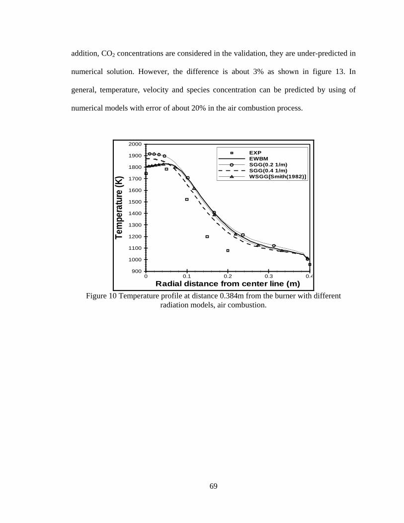
69

addition, CO2 concentrations are considered in the validation, they are under-predicted in

numerical solution. However, the difference is about 3% as shown in figure 13. In

general, temperature, velocity and species concentration can be predicted by using of

numerical models with error of about 20% in the air combustion process.

Radial distance from center line (m)

Tem

pera

ture

(K)

0 0.1 0.2 0.3 0.4900

1000

1100

1200

1300

1400

1500

1600

1700

1800

1900

2000

EXPEWBMSGG(0.2 1/m)SGG(0.4 1/m)WSGG[Smith(1982)]

Figure 10 Temperature profile at distance 0.384m from the burner with different

radiation models, air combustion.

70


Tem

pera

ture

(K)

0 0.1 0.2 0.3 0.4900

1000

1100

1200

1300

1400

1500

1600

1700

1800

1900EXPEWBMSGG(0.2 1/m)SGG(0.4 1/m)WSGG[Smith(1982)]SGG(0.31 1/m)


radiation models, air combustion.


Tem

pera

ture

(K)

0 0.1 0.2 0.3 0.4800850900950

1000105011001150120012501300135014001450150015501600

EXPEWBMSGG(0.2 1/m)SGG(0.4 1/m)WSGG[Smith(1982)]SGG(0.31 1/m)


models, air combustion.

71


CO

2co

ncen

tratio

n

0 0.1 0.2 0.3 0.40

0.025

0.05

0.075

0.1

0.125

0.15

0.175

0.2

EXPEWBM


air combustion. For the oxy-fuel combustion, OF21, figures 14 and 15 show the temperature profile at

distance 0.553m and 1.4m from the burner, respectively. It is found that the temperature

predicted by the exponential wide band model (EWBM) is above the measured values by

3.8% at 0.553 m whereas 15% at 1.4 m. In addition, three grey one clear gas weighted

sum of grey gases model (WSGG), which is introduced by Andersson [43], leads to

temperature results with error of 4% and 12% at distance of 0.553m and 1.4m from the

burner respectively. As shown in figure 15, the accuracy of four grey one clear gas

weighted sum of grey gases model (WSGG) is about +16 %. The temperature computed

by the simple grey gas model (SGG) represented by the effective absorption coefficient

of 0.31 (1/m) deviate by 13% compared to experimental data. The absorption coefficient

of 0.2 (1/m) over-predicts the temperature by 7.5% and 23% at distance 0.553m and

1.4m from the burner, respectively. The more accurate results are obtained if the

72

absorption coefficient of 0.4 (1/m) is used in the solution, the difference did not exceed

+4% at distance 0.553m and +15% at distance 1.4m from the burner. Smith weighted

sum of grey gases model (WSGG) over-predicts the temperature by 5.5% and 19% at

distance 0.553m and 1.4m respectively. It is noted in figure 16 that the computed CO2

concentrations are in good agreement with experimental data and the error less than 5%.


Tem

pera

ture

(K)

0 0.1 0.2 0.3 0.4950

1000

1050

1100

1150

1200

1250

1300

1350

1400

1450EXPEWBMSGG(0.2 1/m)SGG(0.4 1/m)WSGG[Andersson(3+1)]WSGG[Andersson(4+1)]WSGG[Smith(1982)]SGG(0.31 1/m)

Figure 14 Temperature profile at distance 0.553 m for different radiation models, OF21

combustion.

73


Tem

pera

ture

(K)

0 0.1 0.2 0.3 0.4850

900

950

1000

1050

1100

1150

1200

1250

1300EXPEWBMSGG(0.2 1/m)SGG(0.31 1/m)SGG(0.4 1/m)WSGG[Andersson(3+1)]WSGG[Andersson(4+1)]WSGG[Smith(1982)]


models, OF21 combustion.


OF21 combustion.

74

In case of OF27 combustion, it is clear from figure 17 that the exponential wide band

model (EWBM) and the weighted sum of grey gases model (WSGG) over predict the gas

temperature. The maximum deviation in the temperature is found to be 8% in case of the

exponential wide band model (EWBM). It is increased to 22% for three grey one clear

gas weighted sum of grey gases model. However, a little improvement in the accuracy is

noted if four grey one clear gas weighted sum of grey gases model is used and in this

case the error is calculated to be 19%. The results of simple grey gas model (SGG) model

with absorption coefficient of 0.4 (1/m) are in good agreement with the measurements,

the error less than 5%. The absorption coefficient of 0.2 (1/m) over-predicts the results

by 13%. It should be mentioned that the weighted sum of grey gases model (WSGG)

developed by Smith is predicting higher temperature by 13%.


radiation models, OF27 combustion.

75

It is clear from figure 18 that the CO2 concentrations are over-estimated compared to the

measured data and the maximum discrepancy in the results does not exceed 3.7%.


OF27 combustion.

4.5 Assessment of gas radiation models

In the previous section, the results of CFD solution method have been checked and

evaluated. CFD solution includes modeling of fluid flow, turbulence, radiation and

combustion. CFD findings were validated by comparing them with experimental

measurements. The maximum discrepancies of the results were about 20%. There is a

necessity to investigate the behaviors of gas radiation models exclusively. For this

purpose, the measured data of Andersson experiment [42, 49] (i.e. temperature profile,

species concentration and radiation intensities) were used in the analysis. Once the above

76

mentioned properties are known, one can calculate the emissivities and radiation

intensities by different models. Then these computed results should be compared to the

ones measured in the experiment. The gas radiative properties models that used in the

study are;

Leckner model

Perry model

Exponential wide band model (EWBM)

Weighted-sum-of-grey-gases model (WSGG)

The above models are coded and executed for this purpose. Initially, total gas

emissivities as a function of gas temperature for air-firing, OF21 and OF27 were

computed and plotted in figure 19, 20 and 21 respectively. In air combustion situation, it

is noted that the Leckner model predicts the emissivities with error not exceed 5%

compared to exponential wide band model (EWBM). The deviation at temperature above

1000 oC is less than 2%, however, this deviation increases up to 5% at temperature of

700 oC. The Perry model under-estimates the emissivities by 15%. It over-predicts the

emissivities at temperature below 700 oC. For the last model, weighted-sum-of-grey-

gases model (WSGG) introduced by Smith, it is always over-estimating the emissivities

with maximum difference of 8%. It should be mentioned that the Leckner model is

under-predicting the total emissivities at temperature higher than 1200 oC and over-

predicting them below this temperature, the minimum deviation is found at 1200 oC and

it is about 0.3%.

77


models, air combustion In case of OF21, as depicted in figure 20, the difference between exponential wide band

model (EWBM) and Leckner is about 4.6% however, this percentage decreases as

temperature increases and reaches to 0.5% at 1400 oC. The emissivities calculated by

Andersson four grey one clear gas WSGG model are under-predicted by 12.7% at

temperature 1400 oC, however, this error reduced at lower temperatures to reach 0.35%

at 700 oC. In the same trend as in air case, the Perry model under-predicts the total gas

emissivities with error of 39%.

78


models, OF21 combustion

Figure 21 demonstrates the total gas emissivities as a function of gas temperature for

OF27 combustion. It appears that the Leckner model gives higher emissivities than of

exponential wide band model (EWBM). The maximum deviation is about 4%. The Perry

model predicts the lower emissivities by 43.5% at 700 oC. The emissivities of four grey

one clear weighted sum of grey gas model are lower by 20% at temperature of 1400 oC

compared to exponential wide band model. At temperature 700 oC, the error is around

8%.

79


models, OF27 combustion

In addition, the weighted-sum-of-grey-gases models (WSGG) are used to determine the

radiation intensities for air-combustion, OF21 and OF27. The non-correlated formulation

of radiative transfer equation (RTE) given by equation (54) is chosen in the solution.

)1( 1,2/1,1,1,, nnvknbvknnvknvknvk III →−−→−− −+= ττ (54)

The path length is divided into n cells as shown in figure 22 in which the radiation

intensity for each cell can be computed from the neighboring cells.

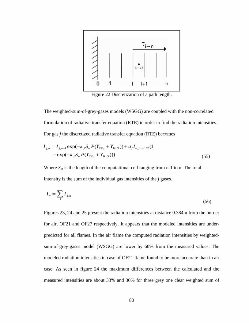
80

Figure 22 Discretization of a path length.

The weighted-sum-of-grey-gases models (WSGG) are coupled with the non-correlated

formulation of radiative transfer equation (RTE) in order to find the radiation intensities.

For gas j the discretized radiative transfer equation (RTE) becomes

(55)

Where Sm is the length of the computational cell ranging from n-1 to n. The total

intensity is the sum of the individual gas intensities of the j gases.

(56)

Figures 23, 24 and 25 present the radiation intensities at distance 0.384m from the burner

for air, OF21 and OF27 respectively. It appears that the modeled intensities are under-

predicted for all flames. In the air flame the computed radiation intensities by weighted-

sum-of-grey-gases model (WSGG) are lower by 60% from the measured values. The

modeled radiation intensities in case of OF21 flame found to be more accurate than in air

case. As seen in figure 24 the maximum differences between the calculated and the

measured intensities are about 33% and 30% for three grey one clear weighted sum of

)))(exp(

1())(exp(

22

22 2/1,,1,,

OHCOmj

njbjOHCOmjnjnj

YYPS

IaYYPSII

+−−

++−= −−

κ

κ

∑=j

njn II ,

81

grey gas model and four grey one clear weighted sum of grey gas model respectively.

The model of three grey one clear weighted sum of grey gas under-predicts the intensities

by approximately 58% for OF27 and this percentage reduced to 56% if four grey one

clear weighted sum of grey gas model is used.



82





At distance 1.4m from the burner the radial radiation intensities are plotted for air, OF21

and OF27 as shown in figure 26, 27 and 28. It is noted that for the air flame the

weighted-sum-of-grey-gases model (WSGG) over-predicts the intensities by 20.7% at the

83

furnace wall. In the OF21 as depicted in figure 27 the modeled intensities by four grey

one clear weighted sum of grey gas model are higher than the measured ones by about

21% and 23% in case of three grey one clear weighted sum of grey gas model. Finally,

OF27 flame intensities are computed and plotted in figure 28, it is found that the

discrepancy in the results of the two models does not exceed 27% compared to the

measured data.



It should be mentioned that the source of errors in the calculated intensities for air and

OF27 at distance 0.384 m is attributed to the soot formation and the high temperature in

this region. As reported by Andersson [49], both the air and OF27 flame display a

luminous appearance due to the soot formed near the burner. Furthermore, it is found that

the volume fraction of the soot particles increases from air to OF27 conditions. On the

other hand, the soot volume fraction is drastically reduced from the air and OF27 flames

84

to the OF21 flame. It can be stated that the differences between the measured total

intensity and the modeled gas intensity is the influence of radiation from soot.





85

CHAPTER 5

CFD MODELING OF A WATER TUBE BOILER UNDER AIR AND OXY-FUEL COMBUSTION

5.1 Introduction

This chapter is aimed at investigating the influence of gas radiation models on

combustion characteristics for full scale fossil fuel furnace. Methane (CH4) is burnt under

three different scenarios (i.e. air, OF21 and OF27). CFD solution of these scenarios

based on different gas radiation models are obtained and discussed. Grid independency

of the results is verified. The error introduced in the results of oxyfuel combustion is

calculated when weighted sum of grey gas model (WSGG), which developed by Smith

for air-fuel combustion, is used. Finally, the characteristics of oxyfuel combustion are

compared to those of air-fuel combustion in this boiler.

5.2 Boiler description

CFD modeling of a full scale fossil-fuel fired furnace is conducted in this study. The

objective of this modeling is to investigate the influence of radiation models on

combustion characteristics and to analyze the impact of replacing air with a mixture of

O2-CO2 in the combustion. The boiler is manufactured by Mitsubishi Heavy Industries

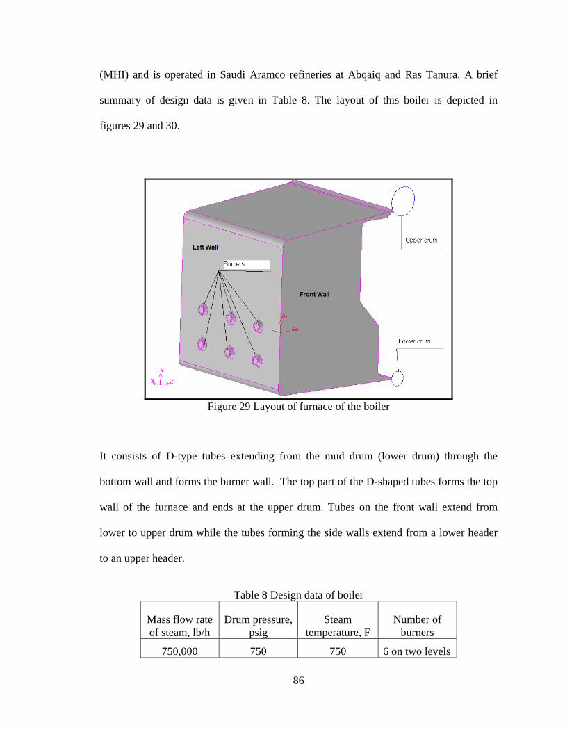
86

(MHI) and is operated in Saudi Aramco refineries at Abqaiq and Ras Tanura. A brief

summary of design data is given in Table 8. The layout of this boiler is depicted in

figures 29 and 30.

Figure 29 Layout of furnace of the boiler

It consists of D-type tubes extending from the mud drum (lower drum) through the

bottom wall and forms the burner wall. The top part of the D-shaped tubes forms the top

wall of the furnace and ends at the upper drum. Tubes on the front wall extend from

lower to upper drum while the tubes forming the side walls extend from a lower header

to an upper header.

Table 8 Design data of boiler

Mass flow rate of steam, lb/h

Drum pressure, psig

Steam temperature, F

Number of burners

750,000 750 750 6 on two levels

87

The water-steam mixture inside the tube is normally saturated and has a saturation

temperature corresponding to the drum pressure. Accordingly, the front, side, rear and

top walls of the furnace provide a constant temperature (538.6 K) boundary condition.

The tubes forming the bottom wall are thermally insulated.

Figure 30 Side view of Furnace of the boiler

It is clear that the boiler consists of 6 burners located in two levels. Each burner has eight

fuel nozzles with 24 fuel jets in each nozzle. The burner construction is shown in Figure

31. This indicates that evaporation may be assumed to start at the beginning of the

sidewalls of the riser tubes. The heat flux imparting on the sidewall causes the quality of

the water/steam mixture to increase as the mixture flows up the riser tubes and also at the

top part of the tubes.

88

Figure 31 burner construction

5.3 Problem setup

The main purpose of this study is to evaluate different gas radiation models and their

influences on the result of air and oxy-fuel combustion scenarios. The study of the full

scale furnace includes three different cases of combustion;

Air combustion ( O2 @ 21 % Vol and N2 @79% Vol )

OF21 (O2 @ 21 % Vol and CO2 @79% Vol )

OF27 (O2 @ 27 % Vol and CO2 @73% Vol )

Methane fuel (CH4) is burnt in the furnace with stoichiometric ratio of about 1.16 (16%

excessive air). It is assumed that all fuel is converted to combustion products of CO2 and

H2O and the total heat input into the furnace is 295 MW. The fuel mass flow rate through

each burner is about 0.98 kg/s. Primary and secondary air passing through each burner

are equal to 8.87 kg/s and 10.7 kg/s respectively. The combustion process takes place in

environment of atmospheric pressure. Computational Fluid Dynamic (CFD) method is

89

used in the solution procedure. Gambit software was used to build a 3-D geometry of the

furnace. The volume of furnace was discretized into 1,335,180 control volumes at which

the solution findings were not affected by the grid (see figures 32 and 33).

Figure 32 General view of the boiler. It is a very important issue in the numerical solution to ensure that the obtained results

are grid independent and this is what will be shown in the next section. All the walls of

furnace are kept at constant temperature of 538.6 K except the bottom wall which is

insulated. Fluent package was utilized in the solution procedure. The summary of the

models and sub-models in the solution as follows:

Incompressible ideal gas assumption

Standard k-ε turbulent model

Temperature-dependent properties

One step volumetric reaction for species transport

90

Finite-rate/Eddy-dissipation turbulence-chemistry interaction

Discrete Ordinate Radiation Model (DO)

Different gas radiative properties models are tested in the solution. In addition to the

models that used in the numerical simulation of the previous chapter, user-defined

functions (UDFs) of Leckner and Perry models were coded and compiled to be used in

the solution.

Figure 33 Closer view of the burners

Since it is required in the radiation modeling, the boiler mean beam length must be

calculated. By using equation (23), the mean beam length of the furnace is found to be

4.5m. In fact, this feature of boiler geometry has a significant effect on the radiation

calculation and the determination of temperature thereafter.

91

5.4 Grid independence study

As mentioned above, all numerical results have to be independent of increasing the

discretization level of certain geometry. The variation of the results with different grids

must be very small and has insignificant impact on them. Once this condition is satisfied,

the results are considered to be grid independent. For this purpose, three different

discretized geometries were examined in this study. They are listed in Table 9.

Table 9 Different grids of the furnace

Grid name Number of cells Percentage of increasing 1 Grid-1 935805 ---- 2 Grid-2 1095555 +17% 3 Grid-3 1335180 +43%

It is found after evaluation and comparison of the obtained results that, in general, the

deviation of the results with increasing the level of discretization above 1335180 cells

will not exceeds 0.01%. Figure 34 shows the temperature profile for the above mentioned

grids along vertical line in the middle between first and second burner near the rear wall

i.e. z =6 m. It is noted that the maximum difference in temperature between Grid-3 and

Grid-2 is about 0.02% and this percentage increased to be 0.07% in the comparison

between Grid-3 and Grid-1.

92

Distance along Y- axis (m)

Tem

pera

ture

(K)

-4 -3 -2 -1 0 1 2 3 41800

1820

1840

1860

1880

1900

1920 Grid-1Grid-2Grid-3

Figure 34 Temperature profile at line (x=3.264, z=6) along Y-axis

In the same manner, the temperature profiles along Z-axis for the three cases were

plotted in figure 35. The maximum variation in temperature between Grid-1 and Grid-3

is calculated to be 1.6% however; it is reduced to 0.2 % in case of Grid-3 compared to

Grid-2. Furthermore, total heat flux has been checked in the analysis. Figure 36

demonstrates the total heat flux along X-axis at line located on the left wall above the

first raw of burners i.e. y= 2 m. it is noted that, the deviation in the results between Grid-

3 compared to Grid-2 is around 0.03% while it becomes 0.06% for Grid-1.

93

Distance along Z-axis (m)

Tem

pera

ture

(K)

0 1 2 3 4 5 6 7200

400

600

800

1000

1200

1400

1600

1800

2000

Grid-1Grid-2Grid-3

Figure 35 Temperature profile at line (x=4.539, y=-2.135) along Z-axis

Distance along X- axis (m)

Tota

lHea

tFlu

x(W

/m2)

1 2 3 4 5 6 7 8-2.5E+05

-2.4E+05

-2.3E+05

-2.2E+05

-2.1E+05

-2.0E+05

-1.9E+05

-1.8E+05

-1.7E+05

-1.6E+05

-1.5E+05

-1.4E+05

-1.3E+05

Grid-1Grid-2Grid-3

Figure 36 Total heat flux profile at line (y=2, z=0) along X-axis

Moreover, the total heat flux profiles along Z-axis at front wall and y=3m are plotted in

figure 37. The difference between Grid-3 and Grid-1 is found to be 0.9%. The deviation

94

of 0.4% is computed for Grid-2 related to Grid-3. It should be mentioned from the above

discussion that the variation in the results if Grid-3 is used in the solution will be

insignificant.

Distance along Z- axis (m)

Tota

lHea

tFlu

x(W

/m2)

1 2 3 4 5 6-3.0E+05

-2.8E+05

-2.6E+05

-2.4E+05

-2.2E+05

-2.0E+05

-1.8E+05

-1.6E+05

-1.4E+05

-1.2E+05

-1.0E+05

-8.0E+04

-6.0E+04

Grid-1Grid-2Grid-3

Figure 37 Total heat flux profile at line (x=0, y=3) along Z-axis

5.5 Results and discussions 5.5.1 Comparisons between gas radiation models

Numerical simulation for air combustion, OF21 combustion and OF27 combustion is

obtained by utilizing fluent packaged software. Different gas radiation models are

coupled with discrete ordinate method to calculate the radiation heat transfer in the

furnace. These models are exponential wide band model (EWBM), Leckner model, Perry

model, weighted sum of grey gas model (WSGG) and simple grey gas model (SGG). The

solution was converged when the summation of the residual in the governing equation at

95

all the domain nodes was less than 0.001%. Various absorption coefficients are examined

in the analysis to determine the optimal value that reflects the same behavior of the

exponential wide band model (EWBM) which is considered the benchmark model.

Temperature profiles at different location along Z- axis are plotted for different models.

They were evaluated and compared to the reference model to check their accuracy. It is

found in the air combustion as shown in figure 39, the weighted sum of grey gas model

(WSGG) introduced by Smith [10] predicts higher temperatures by 0.39% compared to

exponential wide band model (EWBM). Simple grey gas model (SGG) with absorption

coefficient equal to 0.25 (1/m) under-predicts the temperature by 4.5% while the

absorption coefficient of 0.18 (1/m) leads to lower results by 3.3%. The deviation in the

temperature is reduced to 0.37% in case of the absorption coefficient has a value of 0.1

(1/m). Figure 38 represents the temperature profiles along Z-axis at x=4.539m, y=4m; the

maximum difference of 7.2% is computed when the simple grey gas model with

absorption coefficient of 0.25 (1/m) is used in the solution. Weighted sum of grey gas

model is in good agreement with the benchmark solution, i.e. the deviation less than

0.5%. The more accurate results are obtained when the absorption coefficient of 0.1

(1/m) is chosen in the solution, the error less than 0.35%.

96


Tem

pera

ture

(K)

0 1 2 3 4 5 61200

1300

1400

1500

1600

1700

1800

1900

EWBMSGG(0.1 1/m)SGG(0.18 1/m)SGG(0.25 1/m)WSGG


air combustion


Tem

pera

ture

(K)

0 1 2 3 4 5 6 71500

1600

1700

1800

1900

2000

EWBMSGG(0.1 1/m)SGG(0.18 1/m)SGG(0.25 1/m)WSGG

Figure 39 Temperature profile at line (x=3.264, y=-1.0675) along Z-axis,

air combustion

97

In case of OF21 combustion, the temperature distribution at line located in the middle of

the furnace at y=4m along Z-axis is represented in the figure 40. Leckner model, Perry

model, weighted sum of grey gas model (WSGG) are all over-predicting the temperature

by different amounts. The maximum increase in case of Leckner is about 13.5%. The

differences of 4.5% and 1% are calculated for Perry model and weighted sum of grey gas

model (WSGG), respectively. The appropriate value for the absorption coefficient to get

more accurate results is found to be in the range of 0.1 - 0.18 (1/m); the error less than

±1.4%. Figure 41 represents the temperature profile at line located between first and

second columns of burners in the mid-way between the rows of burners along Z- axis

(i.e. x=3.264m, y=-1.0675m), the results of four grey one clear weighted sum of grey gas

model (WSGG) developed by Andersson et al [26] are in good agreement with those

obtained in case of exponential wide band model (EWBM). It over-predicts the

temperature by 1.2%. Leckner model leads to increasing in the temperatures by about

7.9% whereas Perry model over-estimates the results by 2.8%. Simple grey gas model

with absorption coefficient of 0.1 (1/m) gives more accurate results i.e. the difference

less than 0.89%. The results of simple grey gas model with the absorption coefficient

equal to 0.25 (1/m) are under-predicted by 2.1%.

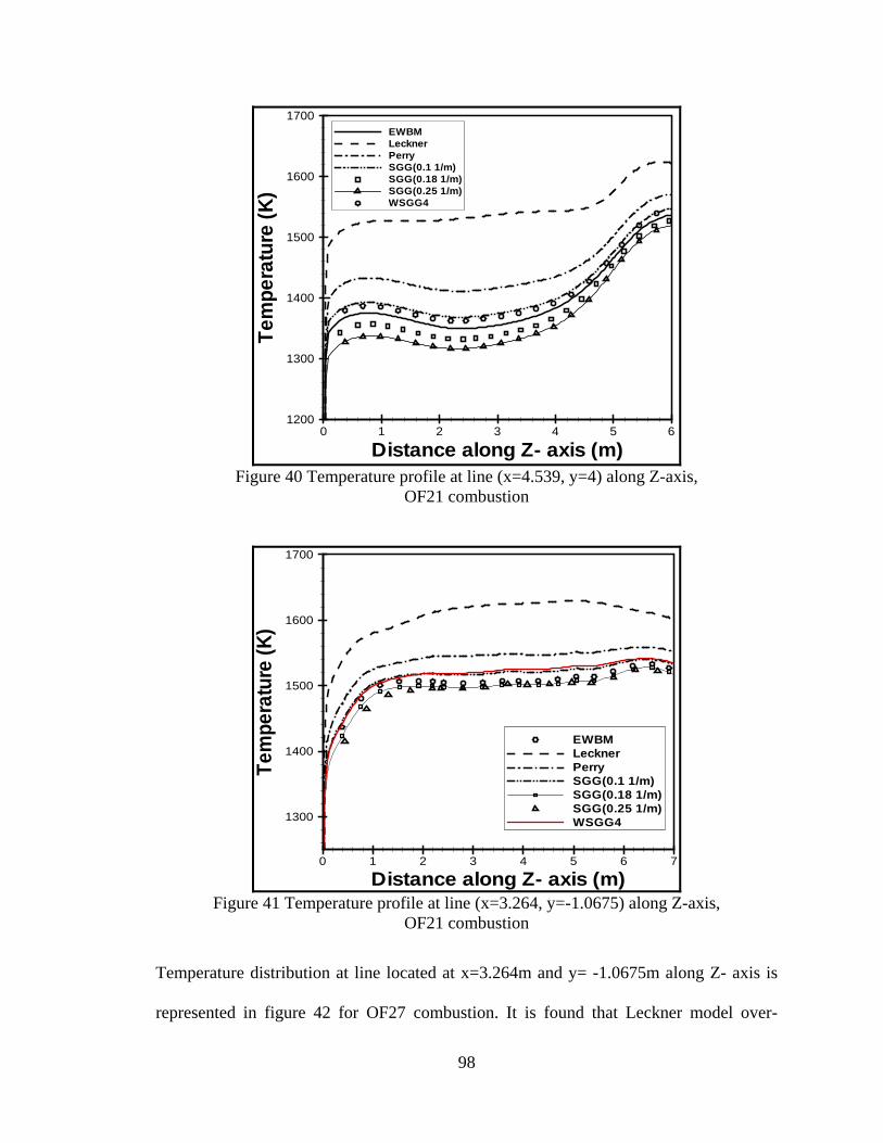
98


Tem

pera

ture

(K)

0 1 2 3 4 5 61200

1300

1400

1500

1600

1700EWBMLecknerPerrySGG(0.1 1/m)SGG(0.18 1/m)SGG(0.25 1/m)WSGG4


OF21 combustion


Tem

pera

ture

(K)

0 1 2 3 4 5 6 7

1300

1400

1500

1600

1700

EWBMLecknerPerrySGG(0.1 1/m)SGG(0.18 1/m)SGG(0.25 1/m)WSGG4


OF21 combustion Temperature distribution at line located at x=3.264m and y= -1.0675m along Z- axis is

represented in figure 42 for OF27 combustion. It is found that Leckner model over-

99

estimates the temperature by 8.6%. The deviation of 2.9% is computed when Perry

model is used. Weighted sum of grey gas model (WSGG) and simple grey gas model

(SGG) with absorption coefficient of 0.1 (1/m) over-predict the temperature by 1%. The

absorption coefficients of 0.25 (1/m) and 0.18 (1/m) are under- estimating the

temperature by1.8% and 0.79% respectively.


Tem

pera

ture

(K)

0 1 2 3 4 5 6 71300

1400

1500

1600

1700

EWBMLecknerPerrySGG(0.1 1/m)SGG(0.18 1/m)SGG(0.25 1/m)WSGG4


OF27 combustion

In addition, temperature distribution at x=4.539m and y=4m along Z- axis is shown in

figure 43. In the same trend Leckner model, Perry model, and weighted sum of grey gas

model (WSGG) are over-predicting the temperature by 15%, 5% and 1.2% respectively.

Simple grey gas model leads to error of 2.8% when absorption coefficient of 0.25 (1/m)

is used and this error is reduced to 1.35% in case the absorption coefficient equal to 0.18

(1/m). It should be emphasized that the maximum difference in the result when the

100

absorption coefficient is selected from the range of 0.25 (1/m) to 0.1 (1/m) will not

exceed 4.3%.


Tem

pera

ture

(K)

0 1 2 3 4 5 61200

1300

1400

1500

1600

1700

1800EWBMLecknerPerrySGG(0.1 1/m)SGG(0.18 1/m)SGG(0.25 1/m)WSGG4


OF27 combustion Weighted sum of grey gas model (WSGG) that developed by Smith [10] is one of the

default model available in the Fluent 6.2. Errors of applying this model for oxyfuel

combustion is calculated and compared to the exponential wide band model (EWBM). It

is found that as shown in figure 44 and figure 45 the predicted CO2 and H2O mole

fractions by these two models for OF27 combustion are in good agreement. The

maximum difference in CO2 mole fraction is less than 0.1% whereas 0.9% in prediction

of the H2O mole fraction.

101

Figure 44 CO2 mole fraction profile at line (x=3.264, y=-1.0675) along Z-axis for

different radiation models, OF27 combustion

Figure 45 H2O mole fraction profile at line (x=3.264, y=-1.0675) along Z-axis for

different radiation models, OF27 combustion Incident radiation profiles at line (x=3.264, y=-1.0675) are plotted in figure 46, the

results of weighted sum of grey gas model (WSGG) are lower by around 31% compared

to the benchmark model (exponential wide band model).

102

Figure 46 Incident radiation profile at line (x=3.264, y=-1.0675) along Z-axis for

different radiation models, OF27 combustion

The influence of radiation models is obvious on the total heat flux on the front wall at

x=0 and y= -1.0675 as shown in figure 47. Weighted sum of grey gas model (WSGG) is

under-predicting the total heat flux by 19%.

Figure 47 Total heat flux profile at line (x=0, y=-1.0675) along Z-axis for different

radiation models, OF27 combustion

103

Temperature profile at line (x=3.264, y=-1.0675) along Z-axis is shown in figure 48, it is

clear that the weighted sum of grey gas model (WSGG) is over-predicting the

temperature by 2.14% in comparison to exponential wide band model (EWBM).

Figure 48 Temperature profile at line (x=3.264, y=-1.0675) along Z-axis for different

radiation models, OF27 combustion. 5.5.2 Characteristics of Oxyfuel and Air-Fuel Combustion Processes

The effect of replacing N2 by CO2 as in the oxyfuel combustion will be discussed for this

boiler. It is clear from the temperature profiles in figure 49 that the temperatures are

lower in the case of oxyfuel combustion compared to air combustion; reduction reaches

up to 21% for OF21 and 18% for OF27. It is thought that the reason of this reduction is

attributed to the higher thermal capacity of CO2 compared to N2. Figure 50 demonstrates

the specific thermal capacity profiles at line (x=3.264, y=-1.0675) along Z-axis for the

air-fuel combustion and the oxyfuel combustion cases, it indicates higher specific

104

thermal capacity in the case of the oxyfuel combustion in comparison to that of air–fuel

combustion. This explains the lower temperature levels in oxyfuel combustion.

Increasing the CO2 recirculation percentage results in higher specific thermal capacity in

the combustion products and, thus, resulting in lower temperature levels. In addition to

this reason, the radiative emissivity and absorptivity of the CO2 is higher when it is

compared to N2 which is transparent to the radiation energy and because of this, flame

cooling effects exhibited in the oxyfuel combustion cases.

Figure 49 Temperature profiles at line (x=3.264, y=-1.0675) along Z-axis for different

combustion cases, EWBM.

Figure 51 shows a comparison between the temperature contours of the air-fuel case and

the two oxyfuel combustion cases. The contours are taken in a vertical plane passing

through the middle burners. It is clear from the figure that the temperature levels in the

oxyfuel combustion cases are lower compared to the air-fuel combustion process. This is

expected as it was explained above that the specific heat capacity in the oxyfuel

105

combustion is higher than that for air-fuel combustion. However, as CO2 mass

percentage is increased, the temperature levels are reduced, as indicated by Figure 51b.

Figure 50 Specific thermal capacity profiles at line (x=3.264, y=-1.0675) along Z-axis for different combustion cases, EWBM.

It is noted that the combustion rate is slower in the case of oxyfuel combustion as

compared to that of air-fired combustion, and this leading to extending the burning zone

causing the flame length to increase. It is also shown that the temperature rise is slower

in the oxyfuel combustion cases in comparison to air-fuel combustion and this is

attributed to the higher specific heat of CO2. Figure 52 shows the contours for

temperature of horizontal plane passing through the upper burners (y=0m)

106

a) Air-fuel combustion

b) Oxyfuel combustion OF21 (21%O2 and 79%CO2 by volume)

c) Oxyfuel combustion OF27 (27%O2 and 73%CO2 by volume)

Figure 51 Contours for temperature of vertical plane passing through the middle burners

2 & 5 (x=4.539m), EWBM

107




Figure 52 Contours for temperature of horizontal plane passing through the upper

burners (y=0m), EWBM.

108

The fuel burning rate is also affected by replacing N2 by CO2. Figure 53 show the

contours of CH4 concentration in the air-fuel combustion and oxyfuel combustion. It is

noted that the fuel consumption rate is slower in the oxyfuel combustion cases. Figure 53

b indicates further reduction in fuel burning rate as the CO2 percentage is increased. In

order to clarify the influence of oxyfuel combustion on the burning rate, the turbulent

viscosity for the cases of air-fuel combustion and oxyfuel combustion were computed.

Figure 54 shows the turbulent viscosity profiles at line (x=3.264, y=-1.0675) along Z-

axis for the three combustion cases. It is noted that the higher turbulent viscosity and

hence higher mixing rates in the case of the oxyfuel combustion in comparison to those

of air-fuel combustion accelerates the reduction in flame temperature and therefore

decreases the fuel consumption rate (i.e. CO2 acts as a cooling gas). This explains the

lower levels of temperature in the oxyfuel combustion.

109




Figure 53 Contours for CH4 mass fraction of vertical plane passing through the middle

burners 2 & 5 (x=4.539m), EWBM.

110

Figure 54 Turbulent viscosity profiles at line (x=3.264, y=-1.0675) along Z-axis for

different combustion cases, EWBM.

Figure 55 shows the contours of the CO2 concentrations of vertical plane passing through

the middle burners 2 & 5 (x=4.539m). The CO2 concentrations rise from around 14% in

the case of air-fuel combustion to above 80% in the oxyfuel combustion in most of the

furnace volume. Figure 56 depicts the density profiles at line (x=3.264, y=-1.0675) along

Z-axis for the three cases, it indicates higher density in the case of oxyfuel combustion

and this is because the molecular weight of CO2 is 44, compared to 28 for N2. This

explains the smaller gas volume exhibited in the oxyfuel combustion cases. The figure

also indicates that the increase in the percentage of CO2 recirculation results in higher gas

density leading to lower radiation rates.

111




Figure 55 Contours for CO2 mass fraction of vertical plane passing through the middle

burners 2 & 5 (x=4.539m), EWBM.

112

Figure 56 Density profiles at line (x=3.264, y=-1.0675) along Z-axis for different


Figures 57 and 58 show the contours of total heat flux (radiative + convective) and

radiation heat flux for air-fuel and oxyfuel combustion at the front, top and left walls of

the furnace. The negative sign of the heat flux means the flux from the walls to the

adjacent gases. Radiation heat flux represents more than 80% of the total heat flux in the

furnace in case of air-fuel combustion and about 70% for oxyfuel combustion and this is

justifying the importance of selecting the appropriate gas radiation models in order to

quantify its value.

113




Figure 57 Contours of radiation heat flux for air-fuel and oxyfuel combustion at the front,

top and left walls of the furnace, EWBM.

114




Figure 58 Contours of total heat flux for air-fuel and oxyfuel combustion at the front, top

and left walls of the furnace, EWBM.

115

It is found that the heat flux on the walls in case of air-fuel combustion is higher than that

for oxyfuel combustion (OF21 and OF27) and this is due to the lower temperature in the

oxyfuel combustion. Total heat flux profiles on the front wall (x=0) and y= -1.0675 along

Z-axis for air-fuel and oxyfuel combustion are plotted in figure 59.

Figure 59 Total heat flux profiles at line (x=0, y=-1.0675) along Z-axis for different


Incident radiation profiles at line (x=3.264, y=-1.0675) along Z-axis for different

combustion cases is shown in figure 60. The high incident radiation in air-fuel

combustion is translated to high temperature of the combustion products. In case of

oxyfuel scenarios and because of replacing N2 by CO2, the incident radiation is reduced

due to the cooling effect of CO2 (i.e. absorbs radiation energy) and this explains the low

temperature in such cases.

116

Figure 60 Incident radiation profiles at line (x=3.264, y=-1.0675) along Z-axis for

different combustion cases, EWBM.

117

CHAPTER 6

CONCLUSIONS AND RECOMMENDATIONS

6.1 Conclusions

Different gas radiation models have been used in CFD modeling of the typical industrial

water tube boiler and their influence on the results was investigated. The characteristics

of oxyfuel combustion are compared to those of air-fuel combustion. The influence of the

CO2 circulation on the oxyfuel combustion characteristics was investigated. Based on the

discussions and analysis of the results, the following can be concluded:

• Leckner model and Perry model are over-predicting the temperature in

comparison to the exponential wide band model.

• Weighted-sum-of-grey-gases model can predict accurate results compared to the

benchmark model, however, it requires new parameters for different ratios of

H2O and CO2. It is a computationally efficient option for CFD simulation where

there is a need for a simple and accurate gas radiation model.

• One of the limitations of Weighted-sum-of-grey-gases model and Perry model is

that they are not applicable for pressure rather than one atmosphere. On the other

hand, the exponential wide band model and Leckner model are valid to be used

for various pressure and ratios of CO2 and H2O.

118

• The influence of these models on the prediction of gases concentrations is very

limited.

• An optimal value for the absorption coefficient can be determined by comparing

the results to the more accurate model (i.e. EWBM).

• The temperature levels are reduced in the case of oxyfuel in comparison to the

air-fuel combustion case.

• Increasing the CO2 recirculation percentage results in higher specific thermal

capacity in the combustion products and, thus, resulting in lower temperature

levels.

• The fuel consumption rates are slower in the oxyfuel combustion case in

comparison to the air-fuel combustion case.

• The energy absorbed is much higher in the case of the air-fuel combustion along

the surfaces.

6.2 Recommendations for future work

Oxyfuel combustion is a promising method to capture carbon dioxide (CO2) and lower

the NOx emission. It is shown from the results that the boiler efficiency is dropped in the

oxyfuel combustion when oxygen (O2) concentration was 27% by volume basis, it is

recommended for further study to investigate the influence of increasing the oxygen (O2)

concentration in the process and its effect on the boiler performance. Furthermore, the

soot radiation impact was ignored in this study and therefore it is very important to

consider its modeling in the future work. Finally, the design features (shape and size) of

119

the boiler play a crucial role in the combustion operation and the boiler overall

performance under air-fuel or oxyfuel conditions.

120

NOMENCLATURE

Iv Spectral radiation intensity [Wm-2sr-1cm-1]

I Total intensity [Wm-2sr-1]

Ib Blackbody intensity [Wm-2sr-1]

Ib, ν Spectral black body intensity [Wm-2sr-1cm-1]

L Path length [m]

c Velocity of radiation [m/s]

Ak Total band absorptance of band k [cm-1]

Pe Equivalent broadening pressure

X Density path-length[g/m2]

PE Effective pressure [bar]

aε,i Emissivity weighting factors for the grey gas i

bε,i, j Emissivity gas temperature polynomial coefficients

aα,i Absorptivity weighting factors

cα,i,j,k Absorptivity polynomial coefficients

Blackbody emissive power [W/(m2.μm)]

Greek symbols

β Mean line-width-to-spacing parameter

ε Emissivity

εc Emissivity of carbon dioxide

εg Total gas emissivity

εw Emissivity of water vapour

ελ Spectral emissivity

ζ Partial pressure ratio

η Pressure corrected line-width-to-spacing parameter

λ Stoichiometric ratio

λmax Pressure correction parameter

kCvoE ,

121

σ Stefan Boltzmann constant [Wm-2K-4]

τ Transmissivity

τH Optical depth at band head

τk Transmissivity of band k

τk, i→n Transmissivity of band k and path i→n

ω Bandwidth parameter [cm-1]

ε0 Zero partial pressure emissivity

ĸv Absorption coefficient [m-1]

σv Scattering coefficient

ηv True emission coefficient

Φv Phase function

α Integrated band intensity[cm-1/(g/m2)]

ω Band width parameter [cm-1]

∆εc+w Overlap between bands of CO2 and H2O

η, µ, ξ Direction cosines

Ω Solid angle [sr]

ρ Reflectivity of the surface

122

References

[1] http://www.esrl.noaa.gov/gmd/aggi/, National Oceanic & Atmospheric Administration, NOAA Research, (visited on December 2010). [2] Jordal K, Anheden M, Yan J, Stromberg L., Oxyfuel combustion for coal-fired power generation with CO2 captures opportunities and challenges, In Seventh conference on greenhouse gas technologies, 2004. [3] Wall T. F., Combustion processes for carbon capture, Proceedings of the Combustion Institute 31 (2007) 31–47. [4] Hadjipaschalis I., Kourtis G., Poullikkas A., Assessment of oxyfuel power generation technologies, Renewable and Sustainable Energy Reviews 13 (2009) 2637–2644 [5] Modest M.F., Zhang H., The full-spectrum correlated-k distribution and its relationship to the weighted-sum-of grey- gas method, in: Proceedings of the 2000 IMECE, vol. HTD-366-1, ASME, Orlando, FL, 2000, pp. 75–84. [6] Hottel H.C., Sarofim A.F., Radiative Transfer, McGraw-Hill, Inc., New York, 1967. [7] Lallemant N., Sayre A., Weber R., Evaluation of emissivity correlations for H2O–CO2–N2/air mixtures and coupling with solution methods of the radiative transfer equation, Progr. Energy Combustion Science, 22 (1996) 543–574. [8] Steward F.R., Kocaefe Y.S., in: U. Grigull, E. Hahne, K. Stephan, J. Straub (Eds.), Proceedings of the 7th International Heat Transfer Conference, vol. 2, Munchen, 1982, pp. 553–558. [9] Steward F.R., Kocaefe Y.S., in: Tien C.L., Carey C.V., Ferel (Eds.), Proceedings of the 8th International Heat Transfer Conference, Hemisphere Publishing Corporation, New York, 1986, pp. 735–740. [10] Smith T.F., Shen Z.F., Fridman J.N., Evaluation of coefficients for the weighted sum of grey gases model, ASME J. Heat Transfer 104 (1982) 602–608. [11] Soufiani A., Djavan E., A comparison between weighted sum-of-gray-gases and statistical narrow-band radiation models for combustion applications, Combustion & Flame 97 (1994) 240–250. [12] Marakis J.G., Kakaras E., Kakatsios X., Papageorgiou N., Application of the direct numerical integration method in a cylindrical geometry containing non-grey pressurized gases, in: Proceedings Eurotherm # 56, Heat Transfer in Radiating and Combusting Systems-3, 1–3 April 1988, Delphy, Greece, pp. 263–274.

http://www.esrl.noaa.gov/gmd/aggi/

http://www.noaa.gov/



http://www.research.noaa.gov/

123

[13] Zhang L., Soufiani A., Taine J., A spectral correlated and non-correlated radiative transfer in a finite axisymmetric system containing an absorbing and emitting real gas– particle mixture, Int. J. Heat Mass Transfer 31 (1988) 2261–2272. [14] Modest M.F., The weighted-sum-of-grey-gases model for arbitrary solution methods in radiative transfer, ASME J. Heat Transfer 113 (3) (1991) 650–656. [15] Denison M.K., Web B.W., A spectral line-based weighted sum-of-grey-gases model for arbitrary RTE solvers, ASME J. Heat Transfer 115 (1993) 1004–1012. [16] Denison M.K., Web B.W., The spectral line-based weighted sum of grey gases model in non-isothermal and non-homogenous media, ASME J. Heat Transfer 117 (1995) 359–363. [17] Pierrot L., Riviere Ph., Soufiany A., Taine J., A fictious gas based absorption distribution function global model for radiative transfer in hot gases, J. Quant. Spectroscopic Radiative Transfer 62 (1999) 609–624. [18] Pierrot L., Soufiany A., Taine J., Accuracy of narrow-band and global models in H2O, CO2 and H2O–CO2 mixtures at high temperatures, J. Quant. Spectroscopic Radiative Transfer 62 (1999) 523–548. [19] Trivic D.N., Mathematical modeling of three-dimensional turbulent flow with combustion and radiation, Ph.D. Thesis, Department of Chemical Engineering, University of New Brunswick, Fredericton, NB, Canada, 1987. [20] Coelho P.J., Numerical simulation of radiative heat transfer from non-grey gases in three-dimensional enclosures, J. Quant. Spectroscopic Radiative Transfer 74 (2002) 307–328. [21] Liu F., Numerical solutions of three-dimensional non-grey gas radiative transfer using the statistical narrow-band model, Trans. ASME 121 (1999) 200–203. [22] Trivic D.N., Modeling of 3-D non-grey gases radiation by coupling the finite volume method with weighted sum of grey gases model, International Journal of Heat and Mass Transfer 47 (2004) 1367–1382. [23] Buhre B.J.P., Elliott L.K., Sheng C.D., Gupta R.P., Wall T.F., Prog. Energy & Combustion Science, 31 (2005) 283–307. [24] Modest M.F., Radiative Heat Transfer, McGraw- Hill Inc., New York, 1993. [25] Kumar R. Renu, Elliott L., Moghtaderi B., Gupta R., Wall T., Differences in Coal Reactivity in Air and Oxy-fuel Conditions and Implications for Coal Burnout. The

124

Clearwater Coal Conference: The 31st International Technical Conference on Coal Utilization and Fuel Systems, Coal Technology: Whats Next? 2006. [26] Haynes B.S., Wagner H.G., Soot formation, Progress in Energy Combustion and Science, 7, (1981), 229-273. [27] Shaddix C.R., Murphy J.J., Coal char combustion reactivity in oxy-fuel applications, Twentieth Pittsburgh Coal Conference, 2003. [28] Kimura K., Omata K., Kiga T., Takano S., Shikisima S., Energy Convers. Manage. 36 (1995) 805–808. [29] Okazaki K., Ando T., Energy 22 (1997) 207–215. [30] Croiset E., Thambimuthu K.V., Fuel 80 (2001) 2117–2121. [31] Croiset E., Thambimuthu K.V., Palmer A., Chem Can. J., Eng. 78 (2000) 402–407. [32] Molburg J.C., Doctor R.C., Brockmeier N.F., Plasynski S., CO2 capture from PC boilers with O2-firing. Eighteenth annual International Pittsburgh Coal Conference 2001. [33] Khare S.P., Wall T.F., Gupta R.P., Elliott L.K., Buhre B.J.P., Oxy-Fuel (O2/CO2, O2/RFG) Technology for Sequestration-Ready CO2 and Emission Compliance. The Clearwater Coal Conference: The 30th International Technical Conference on Coal Utilization and Fuel Systems, Coal Technology: Yesterday–Today–Tomorrow, 2005. [34] Khare S, Wall T, Gupta R, Elliott L, Buhre B.J.P., Retrofitting of air-fired pf plant to oxy-fuel: heat transfer impacts for the furnace and convective pass, and associated oxygen production requirements, 5th Asia-Pacific conference on combustion, Adelaide, 17-20 July 2005. [35] Wall TF, Gupta R, Sheng CD. Calculations of the heat transfer changes for O2/CO2 oxyfuel combustion retrofits of air fired Pf plant with associated recycle ratios and O2 concentrations fed to the boiler, University of Newcastle, Chemical Engineering, NSW 2308, 2003. [36] Payne R., Chen S.L., Wolsky A.M., Richter W.F., CO2 recovery via coal combustion in mixtures of oxygen and recycled flue gas, Combustion Science and Technology, 67 (1989) 1-16. [37] Chui E.H., Douglas M.A., Tan Y., Fuel 82 (2003), 1201. [38] Tan Y, Douglas MA, Thambimuthu KV. CO2 capture using oxygen enhanced combustion strategies for natural-gas power plants. Fuel 81, 2001, 1007–1016.

125

[39] Zheng L, Clements B, Runstedtler A., A generic simulation method for the lower and upper furnace of coal-fired utility boilers using both air firing and oxy-fuel combustion with CO2 recirculation, 27th international technical conference on coal utilization and fuel systems, Clearwater, Florida 2002. [40] Zheng L., Clements B., Douglas MA., Simulation of an oxy-fuel retrofit to a typical 400 MWe utility boiler for CO2 capture, 26th international technical conference on coal utilization and fuel systems, Clearwater, Florida 2001. [41] Leckner B., Spectral and total emissivity of water vapor and carbon dioxide, Combustion & Flame 19 1972, 33–48. [42] Andersson Klas, Johnsson Filip, Flame and radiation characteristics of gas-fired O2/CO2 combustion, Fuel 86 (2007) 656–668. [43] Johansson Robert , Andersson Klas, Leckner Bo, Thunman Henrik, Models for gaseous radiative heat transfer applied to oxy-fuel conditions in boilers, International Journal of Heat and Mass Transfer 53 (2010) 220–230 [44] Leckner B., The spectral and total emissivity of carbon dioxide, Combustion & Flame 17 (1971) 37–44. [45] Grosshandler W.L., Radiative heat transfer in nonhomogeneous gases: a simplified approach, Int. J. Heat Mass Transfer 23 (1980) 1447–1459. [46] Soufiani A., Taine J., High temperature gas radiative property parameters of statistical narrow-band model for H2O, CO2 and CO, and correlated-K model for H2O and CO2, Int. J. Heat Mass Transfer 40 (1997) 987–991. [47] Rivière Ph., Langlois S., Soufiani A., Taine J., An approximate data base of H2O infrared lines for high temperature applications at low resolution, Statistical narrow-band model parameters, J. Quant. Spectroscopic Radiative Transfer 53 (1995) 221–234. [48] Scutaru D., Rosenmann L., Taine J., Approximate intensities of CO2 hot bands at 2.7, 4.3 and 12 lm for high temperature and medium resolution applications, J. Quant. Spectroscopic Radiative Transfer 52 (1994) 765–781. [49] Andersson K., Johansson R., Johnsson F., Leckner B., Soot formation in propane fired oxy-fuel flames, Energy Fuels 22 (2008) 1535-1541. [50] Habib M.A., Ben-Mansour R., Badr H.M., Ahmed S.F., Ghoniem A.F., Computational fluid dynamic simulation of oxyfuel combustion in gas-fired water tube boilers, Computers & Fluids 56 (2012) 152–165.

126

[51] Porter R., Liu F., Pourkashanian M., Williams A., Smith D., Evaluation of solution methods for radiative heat transfer in gaseous oxy-fuel combustion environments, Journal of Quantitative Spectroscopy & Radiative Transfer 111 (2010) 2084–2094. [52] Johansson Robert, Leckner Bo, Andersson Klas, Johnsson Filip, Account for variations in the H2O to CO2 molar ratio when modeling gaseous radiative heat transfer with the weighted-sum-of-grey-gases model, Combustion and Flame 158 (2011) 893–901. [53] Hjärtstam Stefan, Johansson Robert, Andersson Klas, Johnsson Filip, Computational Fluid Dynamics Modeling of Oxy-Fuel Flames: The Role of Soot and Gas Radiation, Energy & Fuels, ef200983e. [54] Raymond Viskanta, Radiative Transfer in Combustion Systems: Fundamentals & Applications, Purdue University, USA. [55] Siegel Robert, Howell John, Thermal Radiation Heat Transfer, Taylor and Francis, New York, 4th Edition, 2002. [56] Sparrow E. M., Cess R. D., Radiation Heat Transfer, McGraw- Hill Inc., New York, 1970. [57] Viskanta R, Menguc MP. , Radiation Heat Transfer in combustion systems, Prog Energy Combustion Science, 1987, 13, 97-160. [58] Viskanta R., Computation of radiative transfer in combustion systems, International Journal of numerical methods for heat and fluid flow, 18, 2008, 415-442. [59] Chandrasekhar, S. Radiative Transfer, Dover Publications, New York, (1960). [60] Edwards, D.K., Molecular gas band radiation, Advances in heat transfer, 12 (1976), 115-193. [61] Liu F., Becker H. A., Bindar Y., A comparative study of radiative heat transfer modeling in gas-fired furnaces using the simple grey gas and the weighted-sum-of-grey-gases models, International journal of heat and mass transfer 41, 1998, 3357-3371. [62] Lallemant, N., Weber, R., A computationally efficient procedure for calculating gas radiative properties using the exponential wide band model, International Journal of Heat Mass Transfer,39 (1996), 3273-3286. [63] Modak, A.T., Radiation from products of combustion, Fire Research, (1979) Vol. 1, pp. 339-61.

127

[64] Hottel, H. C., Noble, J. J., and Sarofim, A. F., 2007, Heat and Mass Transfer, Chapter 5, in Perry’s Chemical Engineers’ Handbook, 8th Edition, Green, D. W., and Perry, R. H (eds.), McGraw-Hill, New York. [65] Grosshandler, W. L., 1993, RADCAL: A Narrow-Band Model for Radiation Calculations in a Combustion Environment, NIST Technical Note 1402. [66] Truelove JS. , A mixed grey gas model for flame radiation, United Kingdom Atomic Energy Authority Report AERER-8494, Harwell, 1976. [67] Andersson Klas, Characterization of oxy-fuel flames – their composition, temperature and radiation, Ph. D. theses, Chalmers University of Technology, Sweden, 2007.

[68] Fluent 6.2 User's Guide, 2003, Fluent Inc., Center Research Park, 10 Cavendish Court, Lebanon, NH 03766, USA.

128

Vita

• Name: Mohammed Ahmad Rajhi

• Nationality: Saudi

• Address: P. O. Box 30942, Jubail 31951, Saudi Arabia

• Email: [email protected]

• Received B. Sc. degree in Mechanical Engineering from King Saud

University in 2005.

• Joined King Fahd University of Petroleum and Minerals, Dhahran,

Saudi Arabia in 2007.

mailto:[email protected]

Documents

Chapter 1 Introduction - KFUPM