Chapter 1 Finding the Optimal Use of a Limited Incomeassets.press.princeton.edu/chapters/s7990.pdf · Chapter 1 Finding the Optimal Use of a Limited Income ... Edgeworth box diagram

Chapter 1

Finding the Optimal Use of a Limited Income

Main 1. More is better.Economic 2. Free choice is a valuable commodity.Concepts 3. Freedom to trade can make everyone better off.

New 1. Indifference curveTerms 2. Diminishing marginal utility

3. Budget constraint4. Optimal use of a limited income5. Pareto efficiency6. Pareto optimal allocation7. Pareto efficient allocation8. Edgeworth box diagram9. Contract curve

10. Compensation principle11. Substitution effect12. Price effect13. Income effect14. Corner solution

The best place to start the study of economics is with a model of con-sumer decisions. Each of us has a limited income and must make choicesabout how best to allocate it among competing uses. Compared to abundle of goods and services that are given to us with a market value of$20,000, most of us would prefer to have a $20,000 income to spend aswe want. Why? Because each of us has different preferences for differentgoods and services, and thus, the “value” of a dollar is higher if we havethe opportunity to spend it as we please. The value of free choice is acentral tenet in economics and provides the basis to understanding theconcept of a demand curve.

I. Indifference Curves

I am going to pursue this problem in a simplified way. There are twogoods, clothing and housing. There are no other uses of income, no sav-ings and no taxes.

a. the main question

A person has $100 to spend during some period. Using the assumptionsbelow, how much does he spend on clothing and housing?

2 | Chapter 1

To answer this question, I need to introduce the concept of an indiffer-ence curve. An indifference curve merely tells us the various combinationsof goods that make a particular consumer indifferent. Consider figure 1-1,panel (a). I assume that we can create a homogeneous unit of clothing,like yards of quality-adjusted material. This measure is shown on thehorizontal axis. I also assume that we can create a homogeneous unit ofhousing, like number of quality-adjusted square feet, which I show alongthe vertical axis. Suppose we consider some combination of clothing andhousing labeled B, which corresponds to 25 units of clothing and 50 unitsof housing. What other combinations of clothing and housing wouldmake this consumer indifferent to this particular allocation?

b. indifference curves slope downward

We know that any bundle that has both more housing and more cloth-ing must be superior to B, and thus, any such bundle cannot be on thesame indifference curve. This inference follows from the axiom “More isbetter.” The combinations of housing and clothing labeled II in the fig-ure denote superior bundles as compared to B. Likewise, our consumercannot be indifferent between the bundle labeled B and any combina-tion of both less housing and less clothing, denoted by area IV in the fig-ure. This means that the indifference curve passing though point B mustpass through areas I and III. In other words, the indifference curve mustbe downsloping from left to right. Panel (b) in figure 1-1 shows one suchindifference curve that satisfies this criterion.

This particular indifference curve is unique to some hypothetical per-son that we are considering. To be concrete, suppose that we are draw-ing an indifference curve for Jane Smith, who in fact possesses thebundle of goods labeled A. This bundle comprises 100 units of housingand 12.5 units of clothing. And suppose that we quiz her as follows: ifwe take away some units of housing, leaving her with only 50 instead of100, how many additional units of clothing would she require in orderto be indifferent to bundle A? We suppose that she answers, 12.5 units,

Assumptions about consumer preferences:1. Each consumer knows his or her preferences and is able to

articulate them so that we can portray them in the form of a chart.2. Preferences are consistent. If a consumer tells us that some bun-

dle of goods A is superior to bundle B, and bundle B is superior tobundle C, then it must follow that A is preferred to C.

3. More is better. Consumers prefer a bundle of goods that hasmore of both goods. Likewise, a bundle with fewer of both goods isinferior.

Optimal Use of a Limited Income | 3

Figure 1-1. The Shape of an Indifference Curve

which I show in the diagram. This corresponds to bundle B. Thus, weknow that bundles A and B must lie on the indifference curve. Note thatover the relevant range, Jane is willing to give up an average of 4 unitsof housing for each unit of clothing she obtains.1

1This is the average trade-off of clothes for housing over the relevant range. The trade-offis different for each individual unit.

4 | Chapter 1

Assuming that we continue asking her questions like this, we coulddraw a line through all the points of her indifference curve, which I labelas U1 in panel (b). That is, U1 describes all the combinations of clothingand housing that make Jane indifferent to bundle A; we can think of allthese combinations as yielding the same utility to her, which is why I usethe letter U to denote the indifference curve.

c. other things to know about indifference curves

A few other features of indifference curves are important to know: they(a) are convex to the origin, (b) are infinite in number, (c) never cross eachother, and (d) different consumers have different indifference curves.

Indifference curves are convex from the origin. This phenomenon is dueto the concept of diminishing marginal utility, meaning that consumersattach a higher value to the first units of consumption of clothing orhousing, and less value to marginal units of clothing or housing oncethey have an abundance of them. Thus, if Jane has lots of housing andlittle clothing, as for example at point A in the figure, she is willing totrade 50 units of housing for 12.5 units of clothing to form bundle B.But once she attains this bundle, she attaches less value to obtaining stillmore clothing and is more reluctant to give up more units of housing.

For example, starting at point B, suppose that we take 25 units of hous-ing from Jane, say from 50 to 25 units in the figure. She requires 25 moreunits of clothing to make her indifferent to bundle B. Bundle C denotes thenew allocation. Over the range B to C, she is willing to sacrifice only 1 unitof housing to receive 1 unit of clothing, on average. Compare this to themove from point A to point B, where she was willing to give up four timesas much housing for each unit of additional clothing, on average. The dif-ference is that at point B, she already has a fair amount of clothing andthus is not willing to give up as much housing to obtain even more clothing.

There are an infinite number of indifference curves. Panel (b) in figure 1-1depicts a single indifference curve for Jane. That is, I started with bundleA and then drew an indifference curve through all the other bundles likeB and C that yield the same utility to her. But suppose that Jane startedwith an allocation of goods labeled D. We know that this bundle ofgoods cannot be on indifference curve U1 because in comparison to bundle B, for example, bundle D has both more clothing and morehousing. Since more is better, then it follows that D must be on a higherindifference curve than B. Following the same reasoning, bundle E mustbe on a lower indifference curve.

If we pursued the same experiment with Jane starting from bundle Das we did when she had bundle A, we could draw a second indifference

curve running through bundle D in the figure. If we do, then we have anindifference curve labeled U2. Similarly, we could draw an indifferencecurve passing through point E, labeled U0. I show these indifferencecurves in figure 1-2, panel (a). U2 is a higher indifference curve than U1,and therefore any combination of housing and clothing on this curve ispreferred to U1. Similarly, U0 is a lower indifference curve than U1, and


Figure 1-2. An Indifference Curve Map

6 | Chapter 1

therefore any combination of clothing and housing on this curve is infe-rior to U1. In reality, there are an infinite number of indifference curves.To keep the figures simple, we normally portray only two or three in therelevant range to illustrate a problem.

Indifference curves do not cross. Each indifference curve is uniformlyhigher than the one below. Why? If they were not depicted this way, theywould violate the rule of consistency. Consider panel (b) in figure 1-2. Inthis figure, I have drawn indifference curve U1 and show points labeled Fand G. I also portray indifference curve U2 passing through point G. Indrawing it this way, I am saying that bundle G yields the same amount ofutility as bundle F. I also am saying that bundle G is the same as bundleH. But how can this be true, since bundle H has more housing and cloth-ing than bundle F? This conundrum violates the consistency rule. We avoidthis problem as long as we ensure that indifference curves never cross.

Note that we can use this same idea to remind ourselves that any bun-dle on a higher indifference curve is superior to any bundle on a lower in-difference curve. Consider panel (a) in figure 1-2. How can we be surethat bundle C is inferior to bundle D? We know this because bundle Coffers the same utility as bundle B because they are on the same indiffer-ence curve. But bundle B clearly is inferior to bundle D because there arefewer units of housing and clothing in bundle B compared to D. Since Cis the same as B, it follows that C also must be inferior to D. This is an-other application of the principle that more is better.

Different consumers have different indifference curves. The indifferencecurves drawn for Jane are specific to her tastes. Ken Jones would have adifferent set of indifference curves depending on his tastes for clothingand housing. The basic look of his indifference curves would be similarto Jane’s (downsloping, convex, etc.), but his trade-off of clothing andhousing very likely would be somewhat different.

II. Gains from Trade Using the Edgeworth Box Diagram

With this small amount of modeling, we already can illustrate an impor-tant principle of economics—namely, the gains that result from trade. Idemonstrate this concept in the simplest possible way. I assume thatthere are only two people, Jane and Ken. I have Cmax units of clothing andHmax units of housing. I want to demonstrate the proposition that if Iallocate these units in any arbitrary way to Ken and Jane, they almostalways will make each other better off by trading. To do this, I need toshow Jane and Ken’s indifference curves on the same picture. This isdone through the use of an Edgeworth box diagram.

As a first step, I write Jane’s indifference curves in figure 1-3, panel(a). I label Cmax and Hmax on the vertical and horizontal axis to remindmyself that this is the maximum amount of clothing and housing avail-able in the problem. In panel (b), I write Ken’s indifference curves, but Ido it in an odd way: I rotate it 180 degrees, so that his origin is diagonalto Jane’s. In this picture, Ken has more clothing and housing as hemoves away from his origin, as depicted by the arrows. Note that I also


Figure 1-3. Jane’s and Ken’s Indifference Curve Maps

8 | Chapter 1

show Cmax and Hmax as the limits in this chart, so that the horizontal andvertical lengths of the axes are the same as Jane’s.

Exercise:Step 1: Draw two sets of indifference curves for Ken and Jane, bothrecognizing the maximum amount of housing and clothing. Drawthem in seperate charts, but draw Ken’s indifference map upside down.

Exercise:Step 2: Slide the two indifference curve maps toward each other untilthey exactly overlap.

a. construction of the box

To create the “box,” simply slide Ken’s indifference curve map until it issuperimposed onto Jane’s. Note that the charts exactly fit together be-cause the lengths of the axes are the same on Jane’s and Ken’s figures. Ishow these charts superimposed in figure 1-4. I label Ken’s indifferencecurves Ki and Jane’s Ji. Larger subscripts denote higher levels of utility.(Note that it is OK that Ken’s and Jane’s indifference curves cross eachother, as long as Jane’s and Ken’s own indifference curves do not cross.)

Figure 1-4. Edgeworth Box Diagram

I want to illustrate the initial amount of clothing and housing that Kenand Jane have to start with. I could portray this allocation anywhere in thebox, because the axes have been drawn so that no matter where I plot apoint, the total amount of clothing and housing must add to the maximumamounts. For illustration, I arbitrarily allocate these goods as described bypoint A as shown in panel (a) of figure 1-5. Jane has lots of housing andnot much clothing, while Ken has lots of clothing and not much housing.


Figure 1-5. Initial Allocation to Ken and Jane

10 | Chapter 1

Exercise:Step 5: Start trading so that the allocation of goods moves toward thecenter of the “cigar.” We do not know how Ken and Jane will work thetrade, but we know that both can be better off by some trade. Considerthe extreme trades first, that is, those that make one consumer muchbetter off but keep the other one at the same level of utility.

Exercise:Step 3: Depict the initial allocation of housing and clothing to Kenand Jane. This allocation is arbitrary; it does not matter where in thebox we start.

Exercise:Step 4: Draw Jane’s and Ken’s indifference curves through point A.

To solve the problem, I reintroduce some indifference curves. Recallthat there are an infinite number of indifference curves for both Ken andJane, and so by definition, we know that each has one curve passingthrough point A; and so I draw these curves as illustrated in panel (b),figure 1-5. Notice that these curves, when superimposed, look like acigar. Ken’s indifference curve is K1 and Jane’s is J1.

b. pareto superior trades

It is immediately apparent that a trade could make either Ken or Jane orboth better off without making either worse off. This trade involvesJane giving some housing to Ken, and Ken giving some clothing to Jane,meaning that the allocation moves in a southeast direction in the figure—that is, toward the fat part of the “cigar.”

For example, suppose that Ken and Jane trade in a way that movestheir allocation from A to B. In this case, Ken is no worse off than at A,because he is on the same indifference curve; but Jane is clearly betteroff because at B she is on a higher indifference curve compared to pointA (compare J4 to J1). When a trade makes at least one participant betteroff and no participant is worse off, then it is said to be Pareto superior.Similarly, they could trade so that Jane is no worse off but Ken is betteroff. Ken gets the best deal without reducing Jane’s utility at point C. Themove from A to C also is Pareto superior. Many moves starting from Aare Pareto superior.

It is not possible to know exactly who is going to get the better dealin a trade. It depends on Jane’s and Ken’s relative bargaining power.Most likely, however, both will gain, and we can characterize the rangeof outcomes in which both can be better off compared to point A.

To do this, I add a few more indifference curves in the relevant rangein panel (a) of figure 1-6. Consider a move from point A to point D. In


Figure 1-6. The Dynamics of Trading: Pareto Efficient Solutions

12 | Chapter 1

Exercise:Step 6: Depict some arbitrary move toward the middle of the “cigar.”Any such move will show that both Ken and Jane will be better off.Draw Ken’s and Jane’s indifference curves through this point.

Exercise:Step 7: The process ends when any further trade reduces the utility ofat least one of the consumers. This occurs where two indifferencecurves just touch, or are tangent to, each other.

c. the contract curve: pareto optimal allocations

Once they reach a point where their indifference curves no longer forma “cigar” but are just tangent, then it is not possible for one to gain byfurther trade without making the other person worse off. One such out-come is depicted by point E. In general, this condition defines a Paretooptimal allocation. A Pareto optimal allocation exists when any possiblemove reduces the welfare of at least one person. Sometimes, a Paretooptimal solution is referred to as a Pareto efficient allocation. Likewise,a Pareto superior move sometimes is referred to as a Pareto efficienttrade.

comparison to point A, both Ken and Jane each are on a higher indiffer-ence curve, and thus both have benefited from the trade. Clearly, themove from A to D represents a Pareto superior move. But at point D,both can trade again to further increase their utility. In general, as longas a “smaller cigar” can fit inside a “larger cigar” then in an Edgeworthbox diagram, both consumers can be made better off by further trading.When does this process stop?

So far, I have portrayed a solution for one arbitrary initial allocationof clothing and housing, namely A. For this allocation, I have shown atleast three possible trading outcomes, namely B, C, and E in panel (a),figure 1-6, whereby at least one consumer is better off and none is worseoff. Depending on how Jane and Ken bargain, we could have a solutionanywhere along the segment CB in the figure. Any point along this seg-ment has the characteristic that Jane’s and Ken’s indifference curves aretangent.

What if the allocation we started with was not A but some other pointin the Edgeworth box, for example, point G in panel (a)? Repeating the

exercise for this allocation would lead us to some solution along the seg-ment IH, which also is a segment along the contract curve.

If we completed many such exercises, we could find many solutionsin the chart, all of which were characterized by the tangency of Ken’sand Jane’s indifference curves. I already have shown two segments alongthis line, namely, CB and IH. If we draw a line connecting all of thesepoints, we have the contract curve in the Edgeworth box, which I showin panel (b), figure 1-6, by the diagonal line connecting the origins of Jane’s and Ken’s indifference curve maps. This line can be smooth ornot so smooth, depending on how the participants’ indifference curveslook.


Exercise:Step 8: Show the contract curve in the Edgeworth box, which depictsthe bundles that are Pareto optimal outcomes, regardless of wherethe original allocation is depicted.

Exercise:To test your understanding of the Edgeworth box, start with a repli-cation of figure 1-5, panel (a). Put a dot anywhere in the Edgeworthbox designating the initial allocation. Draw Ken’s and Jane’s indiffer-ence curves that pass through that point. Unless you know Ken’s andJane’s utility function exactly, there is no way you can exactly repre-sent where these indifference curves lie, but you can draw illustrativeindifference curves for them, paying attention to the rules of indiffer-ence curves that you have learned. You can then bound the solution(best deal for Jane and best deal for Ken) and show the segmentalong the contract curve between these points that represents therange of possible solutions.

Finally, while we have not worried about where Ken and Jane end upon the contract curve, given their initial allocation, in reality it makes adifference to each participant. For example, starting from point A inpanel (a), figure 1-6, it matters to Ken where along the segment CB heends up; he is far better off at C than B. The opposite is true for Jane.The differences in outcomes is one reason why corporations spend largeamounts of money trying to sway contracts in ways that are favorableto them, without at the same time making the deal unprofitable for theother party. Put simply, lawyers and other professionals are paid consid-erable sums to help influence outcomes along the contract curve.

14 | Chapter 1

III. The Budget Line: The Essence of the Economic Problem

In most market settings, individuals are not trading directly with eachother but instead are faced with market prices that are beyond theirinfluence. In addition, their income is given and limited. A consumer’sproblem is to allocate her income among available products and servicesto attain the highest level of utility. In our simple problem where thereare only two goods and no taxes or savings, then we can depict the con-sumer’s budget constraint as follows:

Pareto superior: A trade that makes at least one party better off with-out making anyone worse off.Pareto optimal allocation: Any outcome that cannot be altered withoutmaking at least one person worse off. Sometimes, a Pareto optimal so-lution is referred to as a Pareto efficient allocation. Likewise, a Paretosuperior move sometimes is referred to as a Pareto efficient trade.On the contract curve: A shorthand way of describing a Pareto opti-mum solution; its meaning derives from the Edgeworth box.

Gains from Trade: Lessons from the Edgeworth Box

Even though no new production takes place, Ken and Jane both im-prove their welfare by trading some units of clothing and housing.Both improve the welfare of their trading partner as a by-product ofpursuing their own interests.

In reference to figure 1-6, panel (a), if the initial allocation is de-picted by point A and the final allocation after trading by point E,then both Ken and Jane walk away from the transaction thinkingthey got a good deal. That is, trading is not a zero sum game: tradingcan improve the welfare of all the participants to the trade.

Owing to diminishing marginal utility and the fact that individualsdo not all have the same preferences for goods, an arbitrary alloca-tion of goods to individuals usually is not as good as the allocationthat individuals choose if given the opportunity to trade.

Budget line: I � P� � � PC C

The variable I is the consumer’s income, PH is the price of each unitof housing, PC is the price per unit of clothing, and H and C are theunits of housing and clothing that the consumer purchases.

Figure 1-7, panel (a), illustrates the consumer’s budget. To make theexample concrete, I assume that the price of housing is $1 per unit,


Figure 1-7. Mechanics of the Budget Line

16 | Chapter 1

while the price of clothing is $2 per unit. I also suppose that income is$100. The budget constraint tells us that if the consumer spends all ofher money on housing, she can purchase 100 units; if she allocates allher money to clothing, then she can purchase 50 units. In addition, thebudget constraint describes every other possible allocation of housingand clothing that she can afford. The linear segment in figure 1-7 repre-sents this budget.

a. impact of income changes

The particular budget shown in figure 1-7 assumes an income of $100.Suppose her income doubles to $200 but that the prices of clothing andhousing remain the same. Then the budget line moves parallel to theright, as shown in panel (b). In this case, she now can purchase 200 unitsof housing and no clothing or 100 units of clothing and no housing, orany combination in between, as shown by the income line I = $200.

b. impact of price changes

Alternatively, suppose that the price of clothing falls from $2 to $1, buteverything else stays the same; that is, income is $100 and the price ofhousing is $1. Then, the maximum amount of housing that the con-sumer can purchase still is 100 units. But now she can purchase twice asmany units of clothing if she allocates all her income to clothing. Thismeans that the budget line rotates out in the direction of the price reduc-tion, as illustrated in panel (c).

IV. Consumer Choice: The Optimum Use of a Limited Income

We are now ready to put our model together to determine how Jane al-locates her income between clothing and housing. We merely superim-pose Jane’s budget constraint and indifference curves in the same chart,as shown in figure 1-8, panel (a).

a. determining the optimal solution

We know that Jane must purchase a combination of housing and cloth-ing that is consistent with her budget line; and thus, bundles like A or Fin the figure are possible allocations. Suppose that Jane considersallocation F. This allocation is possible because it lies on her budgetcurve. She enjoys utility level U1. Similarly, she could choose bundle Gthat also gives her utility U1. But she can do better than either of theseallocations.

In particular, at point F, Jane is willing to trade a substantial amount ofhousing to obtain some additional clothing, as depicted by the steepness


Figure 1-8. Optimal Allocation of Income

18 | Chapter 1

of her indifference curve around this point. The budget line is much flatterover this range. More specifically, around point F, in order to obtain onemore unit of housing, Jane is willing to sacrifice about 10 units of hous-ing. But the market prices are such that she is able to obtain 1 more unitof clothing in exchange for only 2 units of housing. So it appears like agood deal to continue giving up housing for clothing at these prices.

Alternatively, you can use the shortcut from the Edgeworth box. Atpoint F, the area bounded by the indifference curve and the budget line(area FEG) looks like a cigar, and F is the tip of the cigar. You know thatshe needs to move toward the center of the cigar. As she trades housingfor clothes at market prices, she goes to a higher utility curve and findsherself at the tip of ever-smaller cigars, until she attains the bundlewhere the budget line and indifference curve are just tangent. Point Adescribes this solution.

More simply still, Jane’s optimal allocation is found by moving alongher budget line until she attains her highest utility. It is apparent frominspection that this solution is depicted by point A in the figure, whereJane’s budget line is tangent to her indifference curve. At point A, it isnot possible for Jane to alter her allocation along her budget line with-out reducing her level of utility.

b. portraying an exact solution

To obtain a specific solution for Jane, I assume that her utility is de-scribed by the following mathematical function, which is a commonexample used for illustration:

Assume that Jane’s utility function is described as follows:

U � C H

Jane’s utility equals the square root of units of clothing consumedtimes the square root of units of housing consumed. For this utility func-tion then, for any given value of U, say U1, then setting C to a series ofvalues from zero to some large number means that H must fall accord-ing to the shape of the indifference curve U1.

2

2This utility function is U � C1/2 H

1/2. At utility level U1, then housing H and clothing C arerelated as follows H � U1

2/C, which defines one indifference curve. To draw utility curves,you can draw out a 45-degrees curve from the origin using a chart like figure 1-8. ForH � C � 1 then U � 1, which you can label U1, then this indifference curve is defined byH � 1/C. Next, H � C � 2 so that U2 � 2, where this indifference curve is defined byH � 4/C, and so on.

Assuming a particular utility function for Jane allows me to find exactsolutions to Jane’s allocation.3 If I assume that her utility function issomewhat different, then I would find some other particular combina-tion of clothing and housing that would maximize the value of her in-come. It turns out that given her tastes, Jane’s optimum use of her $100is to buy 25 units of clothing and 50 units of housing.

At the optimal allocation at point A in panel (a), the slope of her in-difference curves exactly matches the slope of her budget constraint. Inequilibrium, Jane is willing to trade housing for clothing at exactly thesame rate that she is able to at given market prices.4 Since point A is onher budget curve, 25 units of clothing and 50 units of housing exactlyexhaust her income.

Even if he had the same income as Jane, Ken’s allocation likely wouldbe different, unless he happened to have the same tastes for housing andclothing as Jane. For example, given his preferences, he might consume70 units of housing and 15 units of clothing. That is, given the same in-come, consumers often find the highest value of their money by allocat-ing it differently than other consumers.

c. how a change in income affects choice

Now we can reconsider what happens to Jane’s consumption if her in-come increases. Panel (b) in figure 1-8 demonstrates the solution whenher income doubles to $200. At the higher level of income, Jane searchesfor the allocation of clothing and housing that gives her the highest util-ity. This solution is depicted by bundle H in the figure. Notice that at thehigher income level, Jane consumes more units of clothing and housingas compared with bundle A. In general, as long as a good is “normal,”consumers will consume more of it at higher income levels.5


3If I maximize her utility function U � C� H� subject to her income constraintI � PCC � PHH, then I have the first-order condition C � H�, where � � (PH/PC)(�/�).Substituting for C in her budget constraint, I have H* � I/(PH � �PC) � I/PH(1 � �/�).Thus, Jane consumes more housing the lower the price of housing relative to clothing, andthe higher her income. Substituting H* back into her income constraint, I have C* � (I �

PHH*)/PC. Note that when � and � each are 1/2, then her optimal solution always occurswhere she spends 50 percent of her income on each commodity. 4Economists sometimes refer to this condition as one where the ratio of the marginalutility of goods equals the ratio of prices, but I do not use this nomenclature in this book.5There are exceptions; for example, perhaps if consumers have sufficient income, they donot purchase hamburger but replace it with steak. But these exceptions are not importantfor our purposes.

20 | Chapter 1

d. the impact of a price change on the optimum solution

A change in prices also affects Jane’s optimum consumption pattern.Suppose that the price of clothing falls from $2 to 50¢ but everythingelse remains the same. Panel (c) depicts the problem. Point A denotesJane’s original allocation of income. Point B denotes her optimal alloca-tion when the price of clothing falls. Not surprisingly, Jane ends upbuying more units of clothing at the lower price, but it is interesting thatgiven her particular utility function, Jane consumes the same 50 units ofhousing at the lower price of clothings.

If Jane had somewhat different tastes, meaning that her indifferencecurves looked somewhat different from those I depict in the figure, a re-duction in the price of clothing might lead Jane to consume either moreor fewer units of housing. It seems odd that if the price of clothing falls,Jane’s consumption of both clothing and housing could increase; thissounds more like an outcome from an increase in income. This puzzlewill be solved when we look more closely at the nature and conse-quences of the change in the price of clothing.

V. The Compension Principle: The Dollar Value of Changes in Utility

In this section, I want to look more closely at the price change depictedin panel (c), figure 1-8. The price reduction clearly makes Jane better off.Her utility increases as depicted. We know that Jane is better off at thehigher utility, but by how much? While we do not know how to quantify“utils,” it turns out that we can measure this utility change in dollars.

a. valuing the utility change from a price reduction

The most obvious way to measure the dollar value of the price reductionis to reflect on the money Jane saves at the lower price. Jane is purchas-ing 25 units of clothing at price $2. The price then falls from $2 to 50¢.If she continues to consume 25 units of clothing, she has an additional$37.50 to spend ($1.50 times 25 units). In other words, Jane has to bebetter off by at least $37.50. It turns out that she is even better off thanthis. To determine a more precise estimate, ask the following question:What is the maximum amount that Jane would pay Ken if he had thepower to reduce the price of clothing from $2 to 50¢?

Figure 1-9 demonstrates the solution. This figure reproduces panel (c) infigure 1-8, except that it adds two new budgets lines, one passing throughbundle A and another tangent to bundle C. To determine the dollar valueof the utility change, start at the new equilibrium denoted by point B. Atthis equilibrium, Jane enjoys utility level U3. Then ask: At the new prices,how much income would Jane require to attain her old level of utility, U1?

Put differently, how much income would we have to take away fromJane to put her on her old indifference curve? Income changes are repre-sented by parallel shifts in budget lines. Start at point B. Drag Jane’s bud-get line leftward in a parallel way until it just touches her old indifferencecurve—this is the budget line that passes through point C shown in thefigure. It is tangent to U1 at point C.

We now have sufficient information to obtain a dollar value of the util-ity change. At point B, Jane’s income is $100. You can read this incomefrom figure 1-9. The budget line intersects the horizontal axis at 200units. The price of clothing on this line is 50¢. Ergo, her budget is $100.

Similarly, the budget line that passes through point C intersects the hori-zontal axis at 100 units of clothing. The price of clothing on this budgetline also is 50¢. Hence, the income level that defines this budget line is $50.

The dollar value of the increased utility from the price reduction is thedifference between these two amounts, $100 � $50. Put differently, ifKen held the power to change the price of clothing, Jane would be will-ing to pay him an amount up to $50. I obtained this estimate by applyingthe compensation principle; that is, I searched for that level of incomethat restores Jane’s original level of utility.6


Figure 1-9. Effects from a Change in Price of Clothing

6For small price changes it turns out that we obtain a good approximation to this answer bysimply calculating the product of the change in price, times quantity of clothing that Janewas consuming at the original $2 price. For large price changes such as the one I show (from$2 to $0.50), this approximation is too crude. I pursue this issue more carefully in chapter 2.

22 | Chapter 1

Why is the answer not $37.50? This is the dollar amount in Jane’spocket when the price change is announced. At the old prices, she pur-chased 25 units at $2 apiece. Now these units cost $12.50. Ergo, she has$37.50 still in her pocket to purchase more clothing and more housing.The reason this answer is incorrect is that if Jane had a budget of $62.50at the new prices, she could attain a higher level of utility than U1.

This alternative can be shown in figure 1-9 as follows. Drag Jane’sbudget line leftward from point B, but instead of continuing to point C,stop at point A as shown by the dotted-line budget schedule in the figure.This is the budget line at the new prices that permits Jane to purchase thebundle of goods that was optimal under the old prices.

It is evident, however, that faced with this budget constraint, Janewould not consume bundle A, but rather would proceed down the budget

Compensation principle: A change in utility brought about by eithera change in price or other interference to the market can be trans-lated into a dollar value by searching for the increment in incomethat restores the original level of utility.

Consider two jobs for lawyers. One is in the area of contracts, ajob characterized by more or less predictable hours and a relativelylow level of anxiety. The other is in the area of litigation, a job thatinvolves tight deadlines, travel to various court venues, and a highdegree of anxiety. Most lawyers require some pay premium (a “com-pensating differential”) to do litigation over contracts that makes upfor the reduction in utility caused by the rigors of the job. This is anapplication of the compensation principle.

Consider the situation in which a well-meaning mom forces herdaughter, Jane, to attend a ballet performance. Jane does not payanything for the ticket and wasn’t going to do anything that nightanyway. She is visibly upset during the performance and cannot de-scribe how much she hated the experience. Upon leaving, in tears,she accuses her mom of “kidnapping” her and threatens legal action(life in the twenty-first century!). Mom knows that she has imposedsubstantial disutility on Jane and asks how much it would take (indollars and cents) to make things right. Jane says that had momasked her ahead of time how much she would have to pay Jane to ac-company her to the ballet, Jane would have said $200. Assumingthat Jane is honest, we know the dollar value of her reduction in util-ity. Damages after the fact often are illuminated by asking about theprice of a contract that the plaintiff would have required to be ex-posed to the damages that resulted. This is an application of the com-pensation principle.

line to find a higher utility level, U2. The optimum bundle is depicted atpoint D. Comparison of this budget line to her $100 income measures thedifference in utility U2 and U3. We want the dollar value of the change inutility from U1 to U3. To find the true estimate, continue reducing Jane’sincome until it is just tangent to utility level U1, which is shown by bundleC in the figure.

b. anatomy of a price change: income and “price” effects

The work we just did to value the change in Jane’s utility also serves toillustrate the two components of any price change. First, the price ofclothing falls relative to housing, meaning that Jane’s new optimum allo-cation will be more favorable to clothing relative to housing. This iscalled either the substitution effect or, alternatively, the price effect, andis reflected by a move along a single indifference curve. Second, thelower price allows Jane to attain a higher level of utility. This is calledthe income effect and is shown by a parallel shift in budget lines be-tween two indifference curves.

In terms of figure 1-9, the movement from bundle A to C describesthe sole effect of the change in relative prices without commingling itwith the effect of the change in utility. The movement from A to C de-scribes “price effect,” or, alternatively, the “substitution effect.” Moreunits of clothing are consumed and fewer units of housing, as is appar-ent from comparing points A and C. The price effect is always negative.That is, a reduction in the price of clothing leads to an increase in quan-tity consumed, after compensating for the income effect. The move fromC to B denotes the income effect. Normally, the income effect is positivefor both housing and consumption.

It is apparent by inspection that as a result of the price effect, Jane in-creases the quantity of clothes she consumes from 25 to 50 units. As aresult of the income effect, she purchases an additional 50 units ofclothes. In terms of housing, she reduces her quantity consumed from 50units to 25 units, owing to the substitution effect. But she consumes 25more units as a result of the income effect. The income effect exactly off-sets the substitution effect, which is a result specific to her utility func-tion. Other utility functions could generate situations in which either thesubstitution effect dominated the income effect or vice versa.


Anatomy of a price change: If the price of X falls, then, owing to thesubstitution effect (also called the price effect), the quantity of X con-sumed increases. The price effect is always negative. Owing to the in-come effect, ruling out exceptions (which I do in this book), more ofX is purchased as well as more of everything else.

24 | Chapter 1

VI. Applications of the Compensation Principle

a. buckley’s tulips and mums problem

An illustration of the compensation principle is found in an example ofthe harm done by “detrimental reliance” from Frank Buckley’s Con-tracts I class. My interpretation of the problem goes something like this.Frank likes to plant tulips and mums in his garden every year. Tulipbulbs are planted in the fall and bloom in the spring. Mum seeds areplanted in the spring and bloom in the fall. For simplicity, supposethat Frank has $150 to spend on flowers, that there is no way hiswife will give him more flower money, and that there is no chance Frankwill spend less than his full budget. The price of mums and tulips is $1 per pot.

I portray Frank’s indifference curves in figure 1-10, panel (a). Givenhis particular set of indifference curves, it turns out that if the pricesof mums and tulips are the same (which they are in this problem),Frank’s optimal flower bundle has an equal number of mums and tulips.I have drawn a 45-degree line from the origin to make sure that I por-tray his optimal solution along this line (the 45-degree line describesequal numbers of the two kinds of flowers in the garden). Frank’s usualallocation is depicted by point A, where his garden has 75 tulips and 75 mums.

For Frank’s birthday one year (his birthday is in a winter month),Frank’s uncle Dick feels generous and promises Frank an extra $100 tofinance the planting of more flowers in the coming year. Dick promisesto give Frank the gift after he receives his tax refund. Anticipating theextra $100, Frank now has a $250 budget to purchase flowers. I depictthe higher budget line in the figure. Naturally, given Frank’s prefer-ence for symmetry, as reflected in the neat-looking indifference map,he wants to plant 125 mums and 125 tulips with the higher income(point D).

Anticipating the gift, Frank orders 125 mums in the winter for springplanting. After he plants them, Uncle Dick calls, saying that on accountof an unusually small refund this year, he is changing the amount ofFrank’s gift from $100 to zero. But since Frank already has committed$125 of his flower budget, he has only $25 to spend on tulips.

Frank immediately threatens to sue his uncle Dick, claiming substan-tial harm. Dick replies, “How can there be any harm? You still have the$150 you always had.” But harm was imposed. Assuming that we knowexactly how to calculate Frank’s indifference curves, we can calculatethe amount of the harm. Since I assume a particular utility function forFrank, I can find the answer mathematically. You cannot know the exact


7In the example, I suppose that Frank’s utility curve is described by U � M1/2T1/2. His bud-get line is described by $150 � PMM � PTT, where PM and PT are $1. Note that this is thesame utility function that I assigned to Jane, and thus I can use the derivation in note 3 toshow that when prices are equal, Frank always chooses a 50:50 allocation of mums andtulips in his garden.

Figure 1-10. Buckley’s Tulips and Mums Problem

answer by eyeballing panel (a), figure 1-10, but you can show the harmqualitatively.7

26 | Chapter 1

1. Using the Compensation Principle to Calculate DamagesI suppose that after the flower seasons are over by late fall, Uncle Dickthinks about the harm he imposed on his nephew and decides to makeFrank “whole.” We need to figure out how much Dick owes Frank toaccomplish this outcome. To do this, note that the problem arises be-cause Frank relies on his uncle’s promise. But owing to Dick’s unreliablecharacter, Frank ends up with 125 mums and 25 tulips; that is, he stillhas $150 to spend, but he has committed to 125 mums (they cannot bereturned after they have been planted), thereby leaving him with only$25 to purchase tulips. This outcome is depicted by point B in panel (a).

While at first it seems odd that harm has occurred even though nomonetary damages are observed ($150 is $150 according to Uncle Dick),it is apparent that harm has been imposed, because consumers are not in-different to arbitrary allocations of their income. Harm has occurred be-cause Frank’s optimal 50-50 allocation of flowers is more valuable thanthe lopsided look caused by Uncle Dick reneging on his promise.

Frank evaluated point B when he decided on the original allocationof his income, but rejected it in favor of point A. By choosing point A,Frank enjoys U2 units of utility, whereas point B yields only U1 units ofutility. Because of his uncle’s promise and subsequent reneging, Frank isstuck at point B. This explains why Frank is mad, but does not providea dollar value of the loss.

We can determine this amount by using the compensation principle.We ask the question: at what level of income could Frank have attainedutility level U1? To find out, simply drag the $150 income budget lineparallel to the left until it is tangent to utility level U1. This solution isfound at point C (where the budget line is tangent to the indifferencecurve U1). Since I have assumed a particular utility function for Frank, itturns out that this budget line is equivalent to $112.8

In effect Uncle Dick’s unreliability reduced Frank’s income from $150to $112. Put simply, Uncle Dick owes his nephew $38 to compensatehim for the harm done by his untrustworthy act.

In reality, we could not know Frank’s exact indifference curve mapping. But Frank surely does. And so we could imagine Uncle Dick

8The solution is easily determined. Because of the special utility curve I assume for Frank(see prior note), we know that U1 � 1251/2 251/2 � 56. How much income does Frank needto attain 56 utils? We know that if the prices of mums and tulips are the same, then he al-ways chooses an equal number of tulips and mums. Call this variable x. Solve for the valueof x that gives 56 utils: U1 � 56 � x1/2x1/2. Solving for x times the solutions, x � 56. Sincethe price of mums and tulips is $1, then 56 tulips and 56 mums can be obtained with$112. That is, if Frank has $112 he would allocate half to mums and tulips and attain U1.With $150 in income, we know that Frank attains U2. The dollar difference in these twoutility levels is $38.

asking Frank in September after winning some money at the race-track, “Frank, how much would it take to offset the harm I imposed onyou last spring?” Supposing that Frank was totally honest with hisuncle, then if his indifference curves are like those drawn in figure 1-10,he would answer “$38.” Dick forks over this amount. A family quarrelis settled.

The point is general. Anytime that a consumer is pushed away fromhis optimal allocation of income, harm is imposed. In principle, moneydamages from this harm are calculable. While it generally is impossibleto know this number (since the harmed party might overstate his loss), itexplains one reason why your client might be sued for damages evenwhen no dollar loss is visible. Two additional issues, however, must beaddressed before leaving this problem. First, there is often more thanone way to compensate for harm, and thus, it is worth looking for thecheapest settlement amount. Second, we can at least bound the damagesdone to Frank, even if we cannot know his indifference curves.

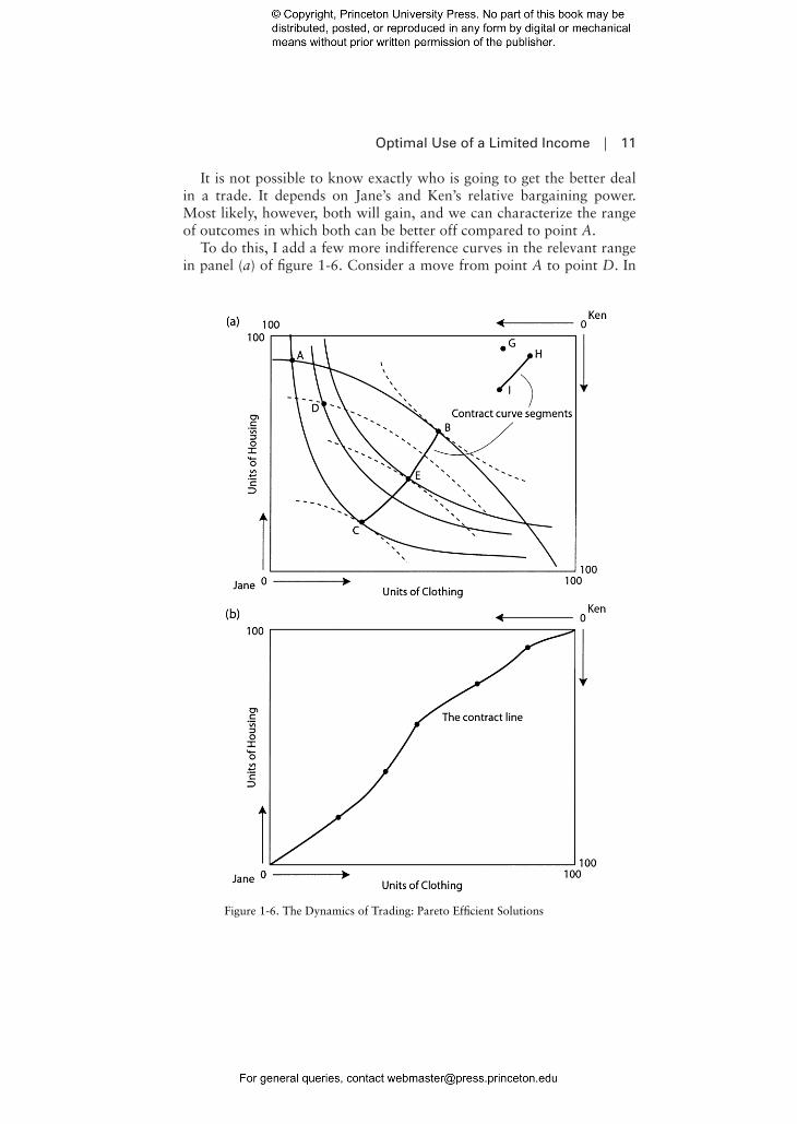
2. A Second Way to Compensate Frank I have supposed that Uncle Dick procrastinates until late fall to compen-sate Frank. We have calculated this amount to be $38. Suppose, how-ever, that Uncle Dick understands the harm he has done in August,when there still is time for Frank to plant more tulips in the fall. In thiscase, it might be cheaper for Uncle Dick to get Frank back onto his util-ity curve U2 right away.

Consider panel (b) in figure 1-10. Dick can do this by purchasingenough extra tulips to move Frank from point B to point E. It turns outthat given the particular indifference curves that I have assumed forFrank, an additional 20 tulips would accomplish this outcome.9

In this case, Uncle Dick makes things right for only $20 instead of$38. This solution is cheaper because Frank attaches some value to theextra 50 mums that Dick induced Frank to purchase, and so adding afew tulips to this burgeoning mums collection is sufficient to makeFrank whole right away. In this case, waiting to settle up would costUncle Dick an extra $18. If, of course, Frank is so mad at Uncle Dickthat he refuses Dick’s offer of $20 worth of tulips right away, then


9Using the particular utility function for Frank as specified in note 7, we know that absentinterference from Dick, Frank would have purchased 75 tulips and 75 mums, and thus,would have attained utility level U2 , which equals U2 � 751/2751/2 � 75. At point B, weknow that Frank is at utility level U1, which as I showed in note 8, equals 56 (U1 � 56).We know that at B, Frank has 125 mums. If he had T tulips, then, together with 125mums, he could attain utility U2 as described at point E. We need to solve for T: U2 �

75 � 1251/2T1/2, which implies T � 45. Since Frank already has 25 tulips at point B, thismeans that Dick can get Frank to point E by giving him 20 more tulips.

28 | Chapter 1

Frank’s claim on Dick is limited to $20.10 So, if Frank cools down onlynext fall, and then demands $38 from Dick, then Dick should give himonly the $20 he originally offered. Frank’s irrational behavior cost himthe $18 difference.

3. Bounding the Solution When Dick Doesn’t Know Frank’s Utility Function

I have supposed that either I know Frank’s indifference curve map or heaccurately portrayed it for me. But suppose that I do not know his map-ping and he is not volunteering the information. He just demands dam-ages in the amount $Z. How can I bound a reasonable estimate on harmimposed by Uncle Dick? One way is to assume that Frank is absolutelycommitted to symmetry in his garden. I defined this condition as fol-lows: Frank always chooses the same number of each flower for his gar-den, regardless of the relative prices between tulips and mums. In thiscase, an additional tulip is worthless unless it is accompanied by an ad-ditional mum and vice versa.11

Figure 1-11, panel (a), portrays these indifference curves. Each utilitycurve is a right angle denoting the idea that given some level of mums,say at point A, no additional number of tulips will add any utility toFrank unless they are accompanied in exact proportion by more mums.Recall that Frank starts out with $150, which corresponds to the pur-chase of 75 tulips and 75 mums in the example (denoted by point A).

10It does not matter whether Dick gives Frank $20 in cash or 20 tulips. In the former case,Frank’s budget shifts outward, but he cannot follow the new budget to find the optimalcombination of flowers because he is stuck at 125 mums, and the best he can do is stop atthis point E, which allows him to enjoy his original level of utility.11This utility function is given by U � a min (T, M), where a is some arbitrary constant.Frank only attaches value to the minimum number of tulips or mums in his garden. If hehas 50 tulips and 30 mums, then any tulips beyond 30 are worthless to him.

Zero substitution: Two goods have zero substitution when, in a com-pensated sense, the consumer always chooses the same bundle ofthese two goods regardless of price.

In the Mums and Tulips problem, Uncle Dick promises Frank an ad-ditional $100, thereby inducing Frank to purchase 125 mums. So, Frankanticipates attaining utility U3 at point D. After Dick reneges, Frankfinds himself at point B in the figure, which describes the purchase of 25tulips and 125 mums. Since he has only 25 tulips, then only 25 mumshave any value to Frank; the remaining 100 might just as well bethrown in the trash. Frank is on indifference curve U1.

It is apparent that Uncle Dick’s untrustworthy behavior has done theequivalent of reducing Frank’s income to $50. At this income level,Frank could have purchased 25 tulips and 25 mums, which would haveput him at point C in the figure, which has the same utility as point B. Inthis case, Dick owes Frank $100: this is the difference between his origi-nal budget curve ($150) and the budget line labeled I � $50 in panel (a).

Note that it is coincidental that the $100 that Dick owes Frank whenthe indifference curves are right angles is the same as the amount of the


Figure 1-11. Bounding the Damage Amount

30 | Chapter 1

gift that Dick promised Frank in the first place. If the price of tulips andmums were different, then the amount that Dick owes Frank would bedifferent from the amount promised.12

If Uncle Dick compensates Frank by buying more tulips before theensuing fall, then he could get Frank back onto his original indifferencecurve by giving him 50 tulips. This compensation moves Frank from B toE in the figure. In this scenario, Uncle Dick salvages 50 of the 125 mumsto which Frank currently attaches no value, by matching them with 50tulips. This solution costs Uncle Dick $50.

Even though we do not know Frank’s indifference curves, we knowthat if Frank attaches a zero value to mums without matching tulips, theshort-run cost is bounded by $50 if Uncle Dick acts before tulip-plantingseason and by $100 if he waits until after the fall season to compensateFrank. This is the upper bound cost of the harm imposed upon Frank.13

The prior analysis gives us the upper bounds on damages. How canwe find the lower bound cost of the harm? We do this by assuming thattulips and mums are perfect substitutes, that is, that Frank enjoys thesame utility no matter what combination of tulips and mums he buys.He is just as happy to have 150 mums and no tulips as he is to have 75 tulips and 75 mums. In this case, his indifference curves are 45-degreedownward-sloping lines from left to right, as shown by the downward-sloping lines in figure 1-11, panel (b). In this case, one of his utilitycurves is coincident with his budget line. Any point along this curvegives Frank the same utility. Suppose he chooses point A arbitrarily.

The fact that his uncle’s promise induces him to purchase 125 mumsis of no consequence, because having 25 tulips and 125 mums is thesame as having 75 of each kind. This solution is depicted by point B inpanel (b), figure 1-11. He has suffered zero utility loss from his uncle’suntrustworthiness. Thus, the lower bound harm is zero.

12For example, if the price of tulips is $2 and the price of mums is $1, then if Frank’s indif-ference curves are right angles his optimal allocation is 50 tulips and 50 mums based onhis $150 flower budget. Let Dick promise Frank $75 and then renege. In this case, youshould be able to show that Frank ends up with 37.5 tulips and 75 mums. He only at-taches value to the first 37.5 mums. He could have purchased 37.5 of each flower for$112.50, and so the harm imposed by Dick on Frank is $37.50 (� $150 � $112.50). Inthis case, the harm is only half of the amount Dick promised Frank. 13There is one other possibility that I have not considered. What if Frank not only attacheszero utility to each mum that comes up without a matching tulip, but also experiences disu-tility from it? One utility function that corresponds with this idea is as follows: U � a min(T,M) � b|T � M|, which says that Frank obtains utility from the minimum number of tulips ormums in his garden and attaches a negative utility to the absolute difference in their num-bers. The values of a and b measure the intensity of Frank’s utility and disutility. In this case,the indifference curves are no longer right angles but evince an angle of less than 45 degrees,forming a kind of “arrow” look, where the arrows are pointed toward the origin.

By bounding the damages, Uncle Dick is in a better position to strikea deal with Frank to make him whole. If the argument takes place whilethere is still time for Frank to buy more tulips, then if Frank is askingfor damages in excess of $50, Dick knows that his nephew is trying topull a fast one. If the argument takes place after the tulip-planting sea-son, then Dick knows that any claim for damages by Frank beyond$100 is a fabrication. Dick might split the difference between the upperand lower bound and offer Frank either $25 before or $50 after thetulip-planting season, depending on when he decides to settle the issue.


The Case for a $50 Upper Limit on the Damage Amount,Regardless of Settlement Time

In the context of the L-shaped indifference curves, I made the argu-ment that if Dick settles up with Frank after the tulip-planting season,he owes Frank $100. But in fact as tulip-planting season approaches,Frank could have purchased an extra $50 of tulips on his own, and inso doing, reattain his old level of utility for a total cost of $50. Hisfailure to do so increases the value of his losses to $100. Hence, an ar-gument can be made that Dick owes Frank the lesser amount and thatFrank himself is responsible for the remainder of his losses.

Alternatively, suppose that Frank’s wife will not give him $50, butjust prior to the tulip-planting season, Frank calls Dick to explain thatan immediate payment of $50 will settle the dispute. Dick ignoresFrank until after the tulip-planting season. In this case, Dick is respon-sible for the $100 losses that develop after the tulip-planting season.

We will revisit this issue in chapter 8 when the notions of contrib-utory negligence and comparative negligence are introduced.

Question 1: Forget about Uncle Dick and suppose that next season,the price of mums is $2 and the price of tulips is $1. Frank has $150to spend. If his preferences are described in panel (a), figure 1-11,how many tulips does he buy? How many mums?14

Question 2: Same problem except now assume that Frank’s indif-ference curves are described by those in panel (b), figure 1-11.15

14With L-shaped indifference curves, Frank always chooses the same number of tulips, T,and mums, M. His budget constraint is $2M � $1T � $150. Since M � T, then Frankbuys 50 mums and 50 tulips. 15Since Frank is indifferent between tulips and mums, then he will purchase 150 tulips andzero mums. That is, if both are interchangeable to Frank, he simply spends all his flowermoney on the cheaper alternative.

32 | Chapter 1

4. The Second-Round Cost of UntrustworthinessAssume that Frank and his uncle settle up for last year’s unfortunateevents. And suppose that next winter, Uncle Dick again promises Franka $100 gift; in fact, he promises to show up with 100 mums for springplanting. He says, “Don’t worry, Frank: this time, I am good for the$100 because I know I am getting a big tax refund.” Figure 1-12 depictsthe emerging problem.

If Frank believes his uncle, then he anticipates a total flower budgetof $250, comprising his regular allocation of $150 plus Dick’s contribu-tion. Frank plans on locating at point D in figure 1-12 next season,which corresponds to 125 tulips and mums and utility level U3. ButFrank no longer trusts his uncle, and so he attaches zero merit to thepromise. So Frank buys 75 mums for spring planting, leaving him withsufficient funds to plant 75 tulips in the fall. He figures on locating atpoint A in the figure.

When spring arrives, however, Uncle Dick comes through with the$100, and in fact, he brings 100 mums for Frank. Now Frank has 175mums and 75 tulips for planting in the fall, which is depicted by point Cin figure 1-12. Surely, Frank is better off than if his uncle did not bringmore flowers, but he is not as well off as he would have been had he

Figure 1-12. Cost of Unreliability

trusted his uncle. Indeed, at point C, Frank is on indifference curve U2,which is lower than U3.

Recall my assumption that because I know Frank’s utility function, Ican figure out the cost of Dick’s unreliability. It is obvious from the fig-ure that Frank could have attained utility level U2 by purchasing anequal number of tulips and mums, which would put him at point B inthe figure. Using Frank’s utility function, I determined that he couldobtain this allocation with only $230. Note that his money budgetamounts to $250. Thus, Uncle Dick’s $100 gift is worth only $80.16 Thisexplains why, when he sees his uncle coming up the driveway with theadditional mums, Frank does not flash a $100 smile, but rather showswhat his uncle perceives to be four-fifths of a $100 smile.

The wedge between the money Dick spent on mums for Frank andthe value that Frank attached to them is a measure of the cost ofuntrustworthiness.


First lesson about reputation value: There is a cost to reneging on acontract because it builds a reputation for unreliability. The benefitsof dealing with an unreliable person are lower than those of dealingwith someone with a reputation for honesty and trustworthiness. Putdifferently, the gains from trade between parties are higher if bothhave a reputation for trustworthiness than if one has a reputation foruntrustworthiness. Hence, we should expect the asset value of repu-tation to be positive. I will return to this theme later in the book.

16Using the utility function I have assumed for Frank as shown in note 7, utility at point Dis U3 � 1251/21251/2 � 125. Utility level at point C is U2 � 751/21751/2 � 115. Thus, ifFrank has x number of tulips and mums, he could attain U2 with the value of x that satis-fies: U2 � x1/2x1/2 � 115 �� x � 115. Since tulips and mums cost $1 apiece, then Frankcan attain this utility with $230 in income.

b. dominic’s report card and computer games

Consider the following problem. Dominic is a pretty good student but isa better student when he gets paid to do well in school. In particular, ifpaid nothing for good grades, he turns in a 3.0 grade point average(GPA). For $300, he works sufficiently hard to earn a 3.5 GPA. For$400, he turns in a 4.0 GPA. He reacts the same way every quarter. Hiseconomist father decides that the $400 is worth the extra GPA and de-cides to pay this amount. Sure enough, the next quarter, Dominic bringshome the desired 4.0.

1. The Solution at FirstDominic decides to allocate the money in the following way: six com-puter games at $50 each, with the remaining money spent on everythingelse. Suppose that we create a composite good to represent “everythingelse” and arbitrarily attach a price of $1 per unit. Thus, with $400, Dominic buys six computer games and 100 units of “everything else.”Assume that Dominic will repeat this allocation every time he gets hispay-for-performance money.

This allocation is depicted in figure 1-13, panel (a). Note that Do-minic’s budget line is labeled $400 and that his optimal consumption isdenoted by point A, which reflects six computer games. So far, every-thing is working out to the satisfaction of Dominic and Dad. It lookslike a Pareto optimum solution.

2. The Problem That Arises A problem arises, however, when Mom discovers how Dominic isspending his money. She feels strongly that he should be limited to threecomputer games per quarter and that he is better off purchasing 250units of other things, like shirts and books. Dad tries to change hermind, explaining that this could turn out to be an expensive restriction,but to no avail. The restriction stands.

When he learns of the newfound restriction, Dominic retorts that ef-fectively Dad is reducing his money payment to $300, even though Dadforks over $400. Accordingly, Dominic delivers a 3.5 GPA next time.

The three-game restriction effectively moves Dominic from point A topoint B. That is, he still is on his $400 budget line, but he is restricted toonly three computer games, leaving him with 250 units of “everythingelse.” Notice that at this point, he no longer is on utility curve U2 but in-stead attains utility level U1. To put a dollar value on this lower utility,Dominic can ask: what level of income would allow me to attain this

34 | Chapter 1

Question: What value did Dominic attach to the restriction of threecomputer games per quarter? Put differently, how much more cash isDad paying Dominic to obtain a 3.5 GPA compared to a world inwhich no restrictions are imposed on his spending?

Answer: Given the previous information, it is apparent that Do-minic attaches a value of $100 to the three-game restriction. Put dif-ferently, to obtain a 3.5 GPA from Dominic, Dad must pay him anextra $100 above the amount that he would have paid for a 3.5 hadMom not imposed a restriction.


Figure 1-13. Report Cards and Computer Games

utility curve without any restrictions on my spending? The answer isfound by dragging his budget line to the left in a parallel way until it isjust tangent to utility curve U1, which is denoted by point D. Since thisbudget line intersects the vertical axis at six games (which cost $50each), we can infer that this new budget line must be $300, whichsquares with Dominic’s response.

36 | Chapter 1

3. The Second-round SolutionDad really wants that 4.0, and so he tries to figure out how to strike a deal with Dominic that respects Mom’s wishes but still results in thedesired GPA.

Question: How much cash does Dad have to pay Dominic to inducehim to produce the 4.0 GPA without violating the three-game restric-tion? While you do not have Dominic’s utility function, you can readthe answer from the information given in panel (a), figure 1-13.

Answer: The answer requires knowledge of Dominic’s utility function.It turns out, given the function I have assumed for him, that Dad mustgive Dominic $950 in cash to push Dominic back to the utility curvethat was attainable with only $400 in cash with no restrictions. Weknow that this is the budget line because it intersects the horizontalaxis at 950 units of the composite good that costs $1 per unit.

Dominic views “other things” as poor substitutes for computergames, and so requires a large number of additional units of otherthings to make him just as happy as he would be with six computergames and only 100 units of everything else. Thus, it turns out thatMom’s restriction cost Dad $550. Dominic is just as well off as hewas when the first contract was made, but now Dad is $550 worse offwithout making Dominic any better off, a clearly inefficient solutionfrom their perspective.

We need to find a point where Dominic is on utility curve U2 and onhis budget line and satisfies the three-game restriction. Clearly, we arenot looking for a tangency solution, because the restriction inhibits usfrom finding an optimum solution.

To find the answer, we need to shift Dominic’s budget line to the rightalong the three-game line until the intersection of the budget line andthe three-game limit touches his original indifference curve U2. In panel(a), figure 1-13, this outcome is denoted by point C. Note that at thisoutcome, Dominic has only three games, so he is not in violation of therestriction, but he now has a sufficiently high income to regain utilitylevel U2. Dad knows that if Dominic attains U2, he gets the 4.0 GPA onthe next report card.

4. The Extreme Case: A Corner SolutionI can expand on this example to illustrate the extreme case of prefer-ence. Suppose that Dominic’s preference for computer games is absolute

in the sense that no matter what the price of games is relative to “allelse,” Dominic always prefers spending all his money on games. This isan even more extreme case than the one depicted in figure 1-11, panel(a), for Frank’s L-shaped utility curves, because the only combinationthat gives Dominic utility is zero units of “other things” and as manygames as his budget permits him to purchase. These utility “curves” areportrayed in panel (b) of figure 1-13 by straight dashed horizontal lines,only some of which I have labeled.

In this utility mapping, more games yield more utility, but no amountof additional units of “all else” confers any utility. Thus, when con-fronted with his $400 budget line, Dominic chooses eight games andzero of everything else. He has a corner solution depicted by point A.


Corner solution: When considering two goods, a corner solution oc-curs when the highest level of utility is found by setting consumptionof one of the goods to zero. These solutions tend to occur when theconsumer views a competing good as a poor substitute for a favoredgood. In figure 1-13, panel (b), we have both a corner solution andzero substitution, meaning that the optimal solution is zero for every-thing else.

Exercise:Consider the real-life case reported in the Washington Post in August 2001. A mentally ill person who could neither hear nor talkwas imprisoned pending a hearing on a trespass case. Let me call thisperson Mr. Smith. The judge dismissed the case, but owing to a pa-perwork mishap, the D.C. prison never released Mr. Smith. Theykept him in the mentally ill section of the D.C. prison for two yearsuntil they realized their error, whereupon he was released. You are his

continued . . .

It is interesting to reconsider his economist dad’s scheme togetherwith his mom’s restriction. If the restriction is three games, then thisputs Dominic at point B in the figure. Dominic values this as the equiv-alent of $150, because he has no use for the additional $250 in cash. Inthis case, he will not deliver even the 3.5 GPA, let alone the 4.0. More-over, as long as Mom’s restriction holds, no amount of money will in-duce Dominic to budge from his 3.0 GPA. The marginal dollars of cashbeyond the $150 he is allowed to spend on games has no value to him.This is an extreme case of the general lesson that income has morevalue to individuals if they have no restrictions on how to spend it.

38 | Chapter 1

Exercise: Continuedlawyer. Assume that the court agrees that the District of Columbiawas grossly negligent in this case. How much does the District ofColumbia owe Mr. Smith? What principle will you invoke to try toconvince a jury that Mr. Smith is owed some amount, X? Keep inmind that Mr. Smith does not work and has never worked. Moreover,no one was dependent on him; indeed, no one ever missed him for twoyears. Mr. Smith had a private cell, and so you can assume that he wasfree of the possibility of attack or personal injury while in jail.17

Economics in a Short Story: A Pareto Optimum Trade

To appreciate economics, and the gains from trade that lie at its core, it is not important to understand complex mathematics andgraphical analysis, nor is it important to understand the businesstransactions involving major corporations or world trade treaties.

continued . . .

17One obvious approach is to invoke the compensation principle. Ask the following questionto the jury: “Ex ante, how much would you have required in compensation to have the op-portunity to be locked up in a prison for fully two years, without contact with the outsideworld?” This is not a silly question. It goes to the amount of money that makes two optionsequally valuable: (1) freedom with all its attendant benefits (and costs) and (2) going toprison for two years and receiving some amount of compensation in the amount X.

Presumably, there is some value of X that Mr. Smith would have agreed to accept inorder to take prison over freedom. Ask yourself the question: would $200,000 make youwilling to accept the jail option? If not, would $500,000 do the trick? Sooner or later, Iwill come to a number that will make the jail option appealing. Ideally, we want the hon-est number that Mr. Smith would have chosen. But he is not capable of telling us. But per-haps we can ask the jury to come up with their own estimates based on the mental exercisethat you ask them to undertake. Will we obtain a perfect number? No. Consider the alter-native: the District of Columbia owes Mr. Smith nothing because he does not work and noone depends on him. If you know that the latter answer cannot be correct, then you arebeginning to understand the compensation principle.

A case that invokes this approach is United States v. McNulty (446 F.Supp. 90). In 1973,Mr. McNulty won about $530,000 (valued in 2001 dollars) in the Irish Sweepstakes, where-upon he deposited his winnings on the Isle of Jersey where secrecy laws put the monjes be-yond the reach of the Internal Revenue Service. He deliberately did not pay taxes. Heapparently had no other assets and no significant income. The IRS brought him to court,whereupon he received a jail sentence for tax evasion. It is unclear when his sentence began,but it ended on January 23, 1978. At this point, the IRS brought him to civil court to obtainan order for Mr. McNulty to repatriate the taxes owed (about $250,000 in 2001 dollars, in-cluding interest and penalties). McNulty refused and was imprisoned for contempt of courtfor five months, whereupon he was released, free from further legal action owing to doublejeopardy. In exchange for these five months, plus the perhaps three or so years he served fortax evasion, McNulty won the rights to the $250,000 he otherwise would have paid the IRS.


Economics in a Short Story: Continued

A Christmas Memory, an autobiographical essay by Truman Capote,conveys its essence. The story is about poor folk who live in Alabamain the midst of the Depression.

In the story, Buddy, who portrays Capote as a boy, lives with hisunderprivileged adult cousin, Miss Sook Falk. She has been endowedwith neither wealth, education, nor ability, but she has lots of love togive Buddy. Upon entering the holiday season, Buddy and his cousindecide to make pecan fruitcakes for about two dozen Americans theyadmire, most of whom they do not know. These people not only in-clude great Americans like the president of the United States, but alsoinclude people who crossed their lives, like the family whose carbroke down in front of their house last year and with whom MissFalk had a very interesting conversation. After collecting their sparedimes, nickels, and pennies, they set out to collect their supplies—some at the store, where real money is required, and some that re-quire climbing over fences to collect pecans that have fallen fromtrees in a local orchard. But the critical input to the fruitcakes is moredifficult to come by—legally anyhow.

So, they set out for a strange place in the middle of the woods,owned by one Mr. Haha Jones, who has some clear stuff in used-overbottles. Upon coming to the door, a giant man howls, “What youwant?” Buddy hides behind his cousin, who says, “Uh, Mr. HahaJones, we need some of your best, uh, stuff.” “What fer?” says Mr.Haha Jones. “Well, we are making fruitcakes, and we need the finestingredients to make them taste just right.” Mr. Jones returns with abottle. Holding it in one hand and holding out the other, he de-mands, “That’ll be two dollars.”18

“Count it out, Buddy,” says Miss Falk, whereupon Buddy startscounting out the amount, one dime, nickel, and penny at a time. Fi-nally, Mr. Haha Jones, who looks like he’s eaten nothing homemade inyears, at least not anything made by a competent cook, says, “Tell yawhat, ma’am, you take this here bottle [and just as she was about torefuse on account of she doesn’t take charity, he continues] . . . you justgive me one of those pecan fruitcakes when you make ’em.” Where-upon, Ms. Falk’s eyes light up. A great smile comes upon her face asshe says, “You mean like a Trade?” “Yes ’um, ma’am, I reckon so,”says Mr. Jones with a slightly less hardened look on his face.

continued . . .

18Quoted remarks are my memory of the exchange. Actual language in the book may differ. See Truman Capote, A Christmas Memory (New York: Scholastic, 1997).

40 | Chapter 1

Economics in a Short Story: Continued

And so, the bottle passes hands. Buddy and Sook, who have so lit-tle cash but are about to be so rich in fruitcakes, have made a dealwith Mr. Haha Jones, who has plenty of two-dollar bills and clearliquid, but so little good food. The trade has made both better off.

As the scene closes, we see Mr. Haha Jones cracking a small smilein the background as Buddy and his cousin laugh, dance, and singtheir way off his property with their prize, thankful that they stillhave enough change to pay the postage that will be due on all thefruitcakes they need to send, except of course the one for Mr. Jones,which she tells Buddy will have “an extra cup of raisons” and nodoubt will be delivered in person.

Most everyone tries to make economics too complicated. Theessence of all economics is contained in the trade between Miss SookFalk and Mr. Haha Jones. It’s all about creating surplus throughtrades. If you keep this in mind, economics will never be hard.

Documents

Chapter 1 Finding the Optimal Use of a Limited Incomeassets.press.princeton.edu/chapters/s7990.pdf · Chapter 1 Finding the Optimal Use of a Limited Income ... Edgeworth box diagram