CHAPTER

12MECHANICALLY STABILIZED

EARTH AND CONCRETERETAINING WALLS

12-1 INTRODUCTION

Retaining walls are used to prevent retained material from assuming its natural slope. Wallstructures are commonly used to support earth, coal, ore piles, and water. Most retainingstructures are vertical or nearly so; however, if the a angle in the Coulomb earth-pressurecoefficient of Eq. (11-3) is larger than 90°, there is a reduction in lateral pressure that can beof substantial importance where the wall is high and a wall tilt into the backfill is acceptable.

Retaining walls may be classified according to how they produce stability:

1. Mechanically reinforced earth—also sometimes called a "gravity" wall2. Gravity—either reinforced earth, masonry, or concrete3. Cantilever—concrete or sheet-pile4. Anchored—sheet-pile and certain configurations of reinforced earth

At present, the mechanically stabilized earth and gravity walls are probably the mostused—particularly for roadwork where deep cuts or hillside road locations require retain-ing walls to hold the earth in place. These walls eliminate the need for using natural slopesand result in savings in both right-of-way costs and fill requirements.

Cantilever walls of reinforced concrete are still fairly common in urban areas becausethey are less susceptible to vandalism and often do not require select backfill. Typically theycompete well in costs where the wall is short (20 to 50 m in length) and not very high (say,under 4 m). They are also widely used for basement walls and the like in buildings.

This chapter will investigate the basic principles of the reinforced earth, gravity, and con-crete cantilever wall; the sheet-pile cantilever and anchored walls will be considered sepa-rately in the next two chapters.

Figure 12-1 The reinforced earth concept. [After Vidal (1969).]

Facingunits

12-2 MECHANICALLY REINFORCED EARTH WALLS

The mechanically reinforced earth wall of Fig. 12-1 uses the principle of placing reinforc-ing into the backfill using devices such as metal strips and rods, geotextile strips and sheetsand grids, or wire grids. There is little conceptual difference in reinforcing soil or concretemasses—reinforcement carries the tension stresses developed by the applied loads for eithermaterial. Bond stresses resist rebar pullout in concrete; soil relies on friction stresses devel-oped based on the angle of friction 5 between soil and reinforcement or a combination offriction and passive resistance with geo- and wire grids.

The principle of reinforced earth is not new. Straw, bamboo rods, and similar alternativematerials have long been used in technologically unsophisticated cultures to reinforce mudbricks and mud walls. Nevertheless, in spite of this long usage French architect H. Vidal wasable to obtain a patent (ca. mid-1960s) on the general configuration of Fig. 12-1, which hetermed "reinforced earth." We see three basic components in this figure:

1. The earth fill—usually select granular material with less than 15 percent passing the No.200 sieve.

2. Reinforcement—strips or rods of metal, strips or sheets of geotextiles, wire grids, or chainlink fencing or geogrids (grids made from plastic) fastened to the facing unit and extendinginto the backfill some distance. Vidal used only metal strips.

3. Facing unit—not necessary but usually used to maintain appearance and to avoid soilerosion between the reinforcements.

(b) Front face of a reinforced earth wall underconstruction for a bridge approach fill usingpatented precast concrete wall face units

(a) Line details of a reinforced earth wall in place

As required

Original groundor other backfillSelect fill

Reinforcing strips

Figure 12-2 Reinforced earth walls.

Facing units

Rankine wedge

These three components are combined to form a wall whose side view is shown in Fig.12-2a. The facing units may be curved or flat metal plates or precast concrete strips or plates(see Fig. 12-2&). Where geotextiles are used the sheet may lap, as in Fig. 12-3, to producethe facing unit.

When wire mesh or or other reinforcement with discontinuities (grid voids) is used, aportion may be bent, similar to the sheet of Fig. 12-3, to form a facing unit. Grid-type

(d) A low reinforced earth wall showing a different concretefacing unit pattern (also patented). Note top cap includesa drainage depression that empties into a drop inlet barelyseen at forward end.

reinforcements strengthen the soil through a combination of friction and passive pressurepullout resistance. The bent-up portion used as a facing piece provides some erosion controluntil the wall is completed.

The exposed reinforcements are usually sprayed with concrete mortar or gunite (materialsimilar to mortar) in lifts to produce a thickness on the order of 150 to 200 mm. This isboth to improve the appearance and to control erosion. For metals this covering also helps

(c) Backside of wall in (b), whichshows the reinforcing stripsattached to the wall face units.Note the drain pipe to carryrunoff from the future roadsurface. Recent rain has erodedsoil beneath reinforcement stripsat wall, which will have to becarefully replaced. Also shownare interlocking dowels andlifting devices (D rings), whichweigh around 2 kips each.

Assumed failureplane

Facingunit

Soil:

Can vary

Figure 12-3 Using geotextile sheets for reinforcement with the facing unit formed by lapping the sheet as shown.Critical dimensions are Le, L'o, and L0. Distances Le and L0 are variable but for this wall produce a constant lengthLcon = L0 + Le. The Rankine p ^ 45° 4- <f>/2 for backfill /3 as shown. Use your program SMTWEDGE (B-7) tofind p, and make a scaled plot to check computed lengths.

control rust, and for geotextiles it provides protection from the ultraviolet rays1 in sunlightand discourages vandalism.

The basic principle2 of reinforced earth is shown in Fig. 12-4 where we see a wall actedon by either the Rankine or Coulomb active earth wedge. Full-scale tests have verified thatthe earth force developed from the active earth wedge at any depth z is carried by reinforcingstrip tension.

Strip tension is developed in the zone outside the active earth wedge from the frictionangle S between strip and soil and the vertical earth pressure yz on the strip. With no lateralearth pressure left to be carried by the wall facings they can be quite thin and flexible withthe principal functions of erosion control and appearance.

The following several factors enter into the design of a reinforced earth wall:

1. Backfill soil is usually specified to be granular; however, recent research indicates thatwe can use cohesive soil if a porous geotextile is used for reinforcement to allow backfilldrainage. This allows one to use the drained friction angle </>' to calculate friction betweenthe soil and reinforcing.

For cohesive materials, either use a narrow vertical back face zone of granular materialor, alternatively, use strips of a permeable geotextile for vertical drainage.

1MoSt geotextiles have a rating of strength loss versus amount of ultraviolet exposure. ASTM D 4355 gives astandard in which geotextile strength loss is reported for 150 hours of exposure.2An extensive literature survey along with a number of applications, primarily in Europe, is given by Ingold (1982).

Pa = active earth forceTi - tension force in reinforcement

strip (if any)

Figure 12-4 The general concept of reinforced earth is that 2 Ti = Pa cos 8, so the earth force against the wall(or facing units) = 0.

2. Backfill soil should be compacted, taking care not to get equipment too close to the facingunit, so that it is not pulled from the reinforcement.

It is also necessary to exercise care with geotextile fabrics not to tear the fabric inthe direction parallel to the wall. A partial tear of this type would reduce the amount oftension the fabric can carry.

3. Tests with experimental walls indicate that the Rankine wedge (of angle p = 45° + </>/2)adequately defines the "soil wedge." This angle should be routinely checked using thetrial wedge method (or computer program) for large backfill /3 angles.

4. The wall should be sufficiently flexible that the active earth pressure wedge forms andany settlement/subsidence does not tear the facing unit from the reinforcement.

5. It is usual to assume all the tension stresses are in the reinforcement outside the assumedsoil wedge zone—typically the distance Le of Fig. 12-5.

6. The wall failure will occur in one of three ways:a. Tension in the reinforcementsb. Bearing-capacity failure of the base soil supporting the wall, as along the baseline AB

of Figs. 12-3 and 12-6.c. Sliding of the full-wall block (ACDB of Fig. 12-6) along base AB.

7. Surcharges (as in Fig. 12-6) are allowed on the backfill. These require analysis to ascer-tain whether they are permanent (such as a roadway) or temporary and where located.For example:a. Temporary surcharges within the reinforcement zone will increase the lateral pressure,

which in turn increases the tension in the reinforcements but does not contribute toreinforcement stability.

Rankine or Coulombactive earth wedge

Wall orfacing units

Alternativebackfill slopes

Note: With sloping backfillZi = average depth to ithreinforcement level

Rankine earth wedge

Check bearing capacity

Figure 12-5 Length of reinforcements L0 = LR + Le as required but must extend beyond Rankine/Coulombearth-pressure wedge.

b. Permanent surcharges within the reinforcement zone will increase the lateral pressureand tension in the reinforcements and will contribute additional vertical pressure forthe reinforcement friction.

c. Temporary or permanent surcharges outside the reinforcement zone contribute a lat-eral pressure, which tends to overturn the wall.In most cases the lateral pressure from a backfill surcharge can be estimated using the

Theory of Elasticity equation [Eq. (11-20)]. One can also use the Boussinesq equationfor vertical pressure, but it may be sufficiently accurate to use the 2 : 1 (2 on 1) method[Eq. (5-2)] adjusted for plane strain to give

where Q = Bq0 for the strip width (side view) and average contact pressure producedby the surcharge; for point loads use either a unit width (0.3 m or 1 ft) orEq. (5-3). Since these two methods give greatly differing vertical pressures(the 2 : 1 is high and Eq. (5-3) is very low) you may have to use somejudgment in what to use—perhaps an average of the two methods.

B = strip width; you are implicitly using L=I unit of width.

Figure 12-6 General wall case with surcharge on backfill as from a road or other construction. Linearizing thesurcharge pressure profile as shown is sufficiently accurate.

Laba and Kennedy (1986) used the 2:1 vertical pressure method [Eq. (5-2)] as shownin Fig. 12-5 with reasonably good results. In this figure Eq. (5-2) is being used to get apressure increase in the zone L\ so that the friction resistance FR for the effective lengths(Le = L\ + L2) is

Fr = tan 8 [(y z + Ag)Z4 + JzL2]

where terms are identified in Fig. 12-5.8. Corrosion may be a factor where metal reinforcements are used. It is common to increase

the theoretical strip thickness somewhat to allow for possible corrosion within the designperiod, which may be on the order of 50 to 100 years.

9. Where aesthetics is critical, a number of concrete facing unit configurations are availablein a wide range of architecturally pleasing facades, which can either outline the wall orblend it into the landscape (Figs. 12-2fe, d).

10. There will be two safety factors SF involved. One SF is used to reduce the ultimatestrength of the reinforcements to a "design" value. The other SF is used to increase thecomputed length Le required to allow for any uncertainty in the backfill properties andsoil-to-reinforcement friction angle S.

Excavate and replace withwell-compacted granularbackfill

Quality granular backfillcompacted as required

Excavateand replace

Rankine/Coulomb pressureprofile

Composite pressureprofile (Rankine/Coulomb + surcharge)

Surcharge pressureprofile

Originalground

Surcharge

Facingunits

12-3 DESIGN OF REINFORCED EARTH WALLS

The design of a reinforced earth wall proceeds basically as follows:

1. Estimate the vertical and horizontal spacing of the reinforcement strips as in Fig. 12-7.Horizontal spacing s is meaningless for both wire grids and geotextile sheets but one mustfind a suitable vertical spacing h for those materials. The vertical spacing may range fromabout 0.2 to 1.5 m (8 to 60 in.) and can vary with depth; the horizontal strip spacing maybe on the order of 0.8 to 1.5 m (30 to 60 in.). The lateral-earth-pressure diagram is basedon a unit width of the wall but is directly proportional to horizontal spacing s.

2. Compute the tensile loads of the several reinforcements as the area of the pressure diagramcontributing to the strip. This calculation can usually be done with sufficient accuracy bycomputing the total lateral pressure at the strip (see Fig. 12-6) level,

qKi = qh + kqh (12-1)

where qn = Rankine or Coulomb lateral earth pressure, taking into account backfillslope and any uniform surcharge

A ^ = lateral pressure from any concentrated backfill surcharge; obtain usingyour computer program SMBLPl

With the average pressure obtained from Eq. (12-1), the strip tensile force can be com-puted as

Tt = AcqKi (12-la)

where Ac = contributory area, computed (including the horizontal spacing s) as

_ hj + hj+i^c — 2

One should routinely make a computational check:

^ T r , = sX (Pah + area of A<? diagram) (12-lfc)

Figure 12-7 Typical range in reinforcement spacing for reinforced earth walls.

constant

Soil

Reinforcements

That is, the sum of the several tensile reinforcement forces should equal the lateral-earth-pressure diagram ratioed from a unit width to the actual reinforcement spacing s.

Although Fig. 12-6 does not show the correct pressure profile for a surcharge qo and/3 > 0 (for that case refer to Fig. ll-9c and use Ka, which includes the effect of /3), it isa common case. The other common case is a sloping backfill (Fig. 11 -9b) but no concen-trated surcharge.

3. Compute the strip lengths Le of Fig. 12-5 that are required to develop a friction resistanceFr = T1 X SF (or ! ,design = ,computed x SF). From these lengths and the Rankine wedgezone we can then determine the overall strip length L0 to use. It is common to use a singlelength for the full wall height so that the assembly crew does not have to be concernedwith using an incorrect length at different elevations; however, this choice is a designer'sprerogative. The friction length is based on soil-to-strip friction of / = tan 6, where 8 =some fraction of cf> such as 1.0,0.8,0.6</>. What to use depends on the roughness of the strip(or geotextile sheet). For rough materials use 8 = 4>; for smooth metal strips use 8 ~ 20to 25°.

For strips of b X Le or geotextile sheets of base width X Le, both sides resist in fric-tion. For round bars the perimeter resists friction. In both cases friction is the product of/ X normal pressure on the reinforcement, computed as po = yn where n = averagedepth from ground surface to reinforcement. Using consistent units, this approach givesthe following reinforcements:

Strip: Fr = 2{yzt){b X L6) tan8 > T1 X SF (l2-2a)

Rod: Fr = irD(yZi)L6tend > T1 X SF (12-26)

Sheet: Fr = 2{yzdi\ x L6) tan 8 > T1 X SF (12-2c)

where b = strip width, D = rod diameter, and 1 = unit sheet width. Manufacturers pro-vide geotextiles in rolls of various lengths and widths.3 For the year 1993 and earlier, theSpecifier's Guide of fabric specifications listed roll dimensions of geotextiles the givenmanufacturer could supply. For 1994 and later, the roll dimensions are no longer supplied.The supplier should be contacted prior to design to see what fabric dimensions can beprovided.

4. Next compute the reinforcement area for strips b X t and for rods with bar diam-eter D. For wire and geotextile grids, obtain the tension force per some unit of width.For geotextile sheets look in the manufacturer's catalog to find a fabric with a suitablestrength.

For these materials a suitable SF must be used to reduce the ultimate tensile strengthof metal strips and bars to a design value or the geotextile strength (which is, by the way,orientation-sensitive) to a design value. For metals it is common to use some SF such as1.5 to 1.67; however, for both metals and geotextiles we can compute an SF based onpartial safety factors as follows:

r a l l o w = Tult (sF i d X SFcr X SFcd X SFbd X SFif X SF^ ) ( 1 2 " 3 )

3The Industrial Fabrics Association International, 345 Cedar St., Suite 800, St. Paul, MN, 55101, Tel. 612-222-2508, publishes a quarterly magazine Geotextile Fabrics Report and an annual Specifier's Guide, which tabulatesavailable geotextile fabrics and select engineering properties such as tensile strength and permeability.

where T ow = allowable tensile stressuIt = ultimate tensile stress

SFid = installation damage factor, 1.1 to 1.5 for geotextiles; 1 for metalSFcr = creep factor (1.0 to 3.0 for geotextiles; 1 for metal)SFCd = factor for chemical damage or corrosion (about 1.0 to 1.5 for geotextiles;

1.0 to 1.2 for metal)SFbd = factor for biological degradation (about 1.0 to 1.3 for geotextiles; 1.0 to

1.2 for metal)SFif = importance factor (1.0 to 1.5)SF , = general factor; (about 1.0 for geotextiles; about 1.3 to 1.4 for metal)

Koerner (1990 in Table 2-12, p. 115) gives some ranges for the partial factors of safety.The preceding values (not all are in his table) can be used, since you have to estimate themanyway.

Let us compute an allowable tensile stress fa for a steel strip based on 350 MPa steel(factors not shown are 1.0) as

f' = 3 5 0 U X L 2 X L 3 = I ^ = 2 0 4 ^ 2 0 0 M P a

Let us now consider a geotextile example. From the 1995 Specifier's Guide we find anAmoco 2044 woven (W) geotextile with a wide-width tensile strength, using the ASTMD 4595 method, of 70.05 kN/m in both the MD (along the roll) and XD (across the roll)directions. The allowable tensile strength is computed using Eq. (12-3). Substituting someestimated values, we obtain

T _ 7 0 0 c 1 _ 70.051 allow /U*UD 1.5 X 2.0 x 1.2 x 1.1 x 1.1 X 1.0 4.356

= 16.08-* 16.0 kN/m

.1 General Comments

For geotextiles we have a problem in that the fabric strength varies

1. Between manufacturers.2. With fabric type and grade. For example, woven fabric is usually stronger than film fabric

and additionally has a larger coefficient of friction.3. With direction. The MD direction {machine direction, also warp; that is, with the roll) is

stronger than (or as strong as) the XD direction {cross-machine, ox fill; that is, across theroll—transverse to the roll length). Sometimes the strength difference is on the order ofXD « 0.5MD. This means that attention to the strength direction during placing may becritical.

We must test (or have tested by the mill, or use an independent testing laboratory) the fabric toobtain the strength, usually in kN/m (or lb/in.) of width. From the several choices we choosea strip so that

Strip width b X design strength/unit width > Ti

Strip design may require several iterations to set the horizontal and vertical reinforcementspacing. Since fabric cost is relatively small compared with other costs (engineering time,backfill, etc.) and since there is some uncertainty in this type of analysis, a modest amountof overdesign is acceptable.

Metal reinforcement strips currently available are on the order of b = 75 to 100 mm and ton the order of 3 to 5 mm, with 1 mm on each face excluded for corrosion. Concrete reinforc-ing rods are often used for their roughness, but with one end prepared for attachment to theface piece—by welding or threads. Rod diameters should be at least three times larger thanthe average (D50) particle diameters of the granular backfill so adequate friction contact isdeveloped. Particle diameter is less critical with wire grids since the grid bars perpendicularto the tension rods provide considerable additional pullout resistance.

The pullout forces and resistance are assumed to be developed as shown in Fig. 12-4 wherea tension from the wall face to the Rankine/Coulomb rupture zone defined by the angle pdevelops to a maximum at the wedge line. Even with a sloping backfill and/or surcharges theRankine wedge shown is generally used. This tension is resisted by the friction developingoutside the zone along length Le of Fig. 12-5, so we can write, from the differential equationshown on Fig. 12-4,

C Le

T = 2b(po tan 8) d LJo

This expression may be somewhat of a simplification, and 2b must be replaced with theperimeter (TTD) for round bars, but it seems to allow an adequate wall design.

Most of the construction technology currently used for reinforced earth walls is underpatent protection; however, it is important to understand the principles involved and methodsof analysis both in order to make a reasonable decision on the best system for a site andbecause the patents on some of the walls will expire shortly and the method(s) will transferto the public domain.

12-3.2 Soil Nailing

Using "nails" to reinforce the earth is a relatively recent (about 20 years old) method for soilreinforcement. Basically this consists in either driving small-diameter rods (on the order of25 to 30 mm) into the earth or drilling holes on the order of 150 to 200 mm, inserting therequired diameter (again 25- to 30-mm) rod, and filling the remainder of the hole with grout(usually a cement-sand mixture with a low enough viscosity that it can be pumped).

The essential difference between soil nailing and tieback walls (of Chap. 14) is that thereis little prestress applied to the soil nails, whereas the tieback wall requires prestressing therods.

Soil nailing has the advantage of being suitable both for walls and for excavation support.For walls one starts the wall upward and at specified levels inserts "nails" into the backfill.The wall then proceeds and the nail is attached to the wall (often through a prepared hole witha face plate and a nut for fastening). In excavations some depth is excavated, the nails areinserted, and wall is added and attached as for the retaining wall. The next level is excavated,nails are inserted, wall facing is added and attached, etc.

The rods are usually inserted or drilled at a slope from the horizontal of about 15°, butnear the upper part of the wall the slope may be larger (20 to 25°) to avoid underground util-ities.

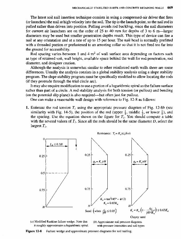
Figure 12-8 Failure wedge and approximate pressure diagrams for soil nailing.

(a) Modified Rankine failure wedge. Note thatit roughly approximates a logarithmic spiral.

(b) Approximate soil pressure diagramswith pressure intensities and soil types

Clayey sand

Sand when

Resistance:

The latest soil nail insertion technique consists in using a compressed-air driver that fires(or launches) the nail at high velocity into the soil. The tip is the launch point, so the nail rod ispulled rather than driven into position. Pulling avoids rod buckling, since the nail diametersfor current air launchers are on the order of 25 to 40 mm for depths of 3 to 6 m—largerdiameters may be used but smaller penetration depths result. This type of device can fire anail at any orientation and at a rate of up to 15 per hour. The nail head is normally prefittedwith a threaded portion or prefastened to an arresting collar so that it is not fired too far intothe ground for accessibility.

Rod spacing varies between 1 and 4 m2 of wall surface area depending on factors suchas type of retained soil, wall height, available space behind the wall for rod penetration, roddiameter, and designer caution.

Although the analysis is somewhat similar to other reinforced earth walls there are somedifferences. Usually the analysis consists in a global stability analysis using a slope stabilityprogram. The slope stability program must be specifically modified to allow locating the rods(if they protrude through the trial circle arc).

It may also require modification to use a portion of a logarithmic spiral as the failure surfacerather than part of a circle. A rod stability analysis for both tension (or pullout) and bending(on the potential slip plane) is also required—but often just for pullout.

One can make a reasonable wall design with reference to Fig. 12-8 as follows:

1. Estimate the rod tension Ti using the appropriate pressure diagram of Fig. 12-8& (seesimilarity with Fig. 14-5), the position of the rod (upper \, middle \, or lower | ) , andthe spacing. Use the equation shown on the figure for J1-. You should compute a tablewith the several values of Tt. Since all the rods should be the same diameter D, select thelargest T/.

2. Compute the required rod diameter D for this tension using a suitable SF so that fa =fy/SF of rod steel (or other rod material). With T1 and fa, compute

D = V 0.7854/.

3. Estimate the nail friction resistance (outside the modified Rankine wedge zone of Fig.12-Sa) using Eq. (Yl-Ib). Use the actual rod diameter if the rod is driven, but use thegrouted diameter if the rod is put in a drilled hole and grouted. Use tan S = estimatedvalue for soil-metal interface based on metal roughness. Use S = </> for grouted rods. Forsloping rods use an average depth zt in the length outside the wedge zone. One must usea trial process for finding the computed distance Le>comp—that is, assume a length andcompute the resistance Fr > Tt. Several values may be tried, depending on whether allrods are to be the same length, or variable lengths (depending on wall location) are to beused. In any case increase the computed length as

^e,des — o r * /^,comp

Compute the total rod (nail) length Z401 at any location as the length just computed for pull-out resistance L^des + length LR to penetrate through the Rankine wedge zone, giving thefollowing:

^tot — Ledes + LR

It will be useful to make a table of nail lengths Ltot versus depth z to obtain the final designlength(s). One has the option of either using a single nail length or of locating elevationswhere the nail length changes occur if different nail lengths are used.

4. Make a scaled plot of the wall height, modified Rankine wedge, rod locations, and theirslopes and lengths. Use this plot to make your slope stability analysis. Clearly one possi-bility is to use a regular slope stability computer program and ignore the "nails."

There is already an enormous amount of literature as well as at least three separate designprocedures for nailed walls. The reader is referred to Jewell and Pedley (1992), Juran et al.(1990) and ASCE Geotechnical SP No. 12 (1987) for design information sources or to buildconfidence in the procedure outlined above.

12-3.3 Examples

We will examine the reinforced earth methodology further in the following three examples.

Example 12-1. Analyze the wall of Fig. E12-1 using strip reinforcement. The strips will be ten-tatively spaced at s = I m and h = 1 m and centered on the concrete wall facing units. We willuse interlocking reinforced concrete facing units, shaped as indicated, that are 200 mm thick (witha mass of about 1000 kg or 9.807 kN each). A wall footing will be poured to provide alignment andto spread the facing unit load somewhat, since their total mass is more than an equivalent volumeof soil. A 150-mm thick reinforced cap will be placed on top of the wall to maintain top alignmentand appearance.

Required. Analyze a typical interior vertical section and select tension strips based on fy =250 MPa and fa = 250/1.786 = 140 MPa. Other data: <j> = 34°; y = 17.30 kN/m3; and assume8 = 0.7 X 34 = 24°.

Solution. From Table 11-3 obtain Ka = 0.283

/ = tanS-> tan 24° = 0.445

Set up the following table from wall data (Le is computed after Tt and strip width b are computed):

~ T1 x SFStrip Z19 T1 = yzid x l)Ka9 U = 2btan8iyzi)9

no. m kN m

1 0.5 2.45 4.772 1.5 7.34 t3 2.5 12.24 I4 3.5 17.14 I5 4.5 22.03 I6 5.5 26.93 |7 6.5 31.82 I8 7.5 36.72 |9 8.5 41.62 I

10 9.5 46.51 4.77XT; =244.80kN

Check:

pa = \yH2Ka [Eq. (11-9) and s = 1 m = unit width]

Pa = i(17.30)(102)(0.283) = 244.80 kN/m

Next we find the cross section of the reinforcement strips. Tentatively try b = 100 mm since thewall is 10 m high.

b x t X fa = T1 (a SF is already on fa)

The largest Tt is strip 10, so for T\o we have

0.100(0(140) = 46.51 kN (using meters)

Figure E12-1

Wall footing Original ground

Reinforcement lug

Facing unit (interlocks not shown)

Select backfill

150 mm top cap

Solving (and inserting 1000 to convert MPa to KPa), we obtain

46 51' = 0.10(140)1000 " 0 0 ° 3 3 2 m ^ 3.32 mm, so use t = 5.0 mm

This value allows a little less than 1-mm loss on each side for corrosion. Next find the strip lengthfor Tt and total strip length L0. We equate tan 8 X vertical pressure po on both sides of strip of widthb X Le to the strip tension T1 X SF. Get T1 from the preceding table and use an SF = 1.5:

2b(tmS)(y Zt)L6 = T1(SF)

Rearranging into solution form for Le, we have

= (SF)Tj = 1.5Tj2b(\an8)(yzi) 2(0.10)(0.445 X 17.3Oz1-)

This equation can be programmed. The first value (for n = 0.50 m) is

1.5(2.45)Le= 1.5397(0.50) = 4 - 7 ? m

Other values for z/ = 1.5, 2.5, 3 .5 , . . . , 9.5 are similarly computed and we find them constant asshown in the preceding table. We now find total strip lengths L0 as follows:

p = 45° + 4>/2 = 45° + 34°/2 = 62°

The Rankine zone at 9.5 m (strip 1) is

LR = 9.5 x tan(90° - 62°) = 9.5 X tan 28° = 5.05 m

L0 = LR + Le = 5.05 + 4.77 = 9.82 m

We can use this length for all of the strips or, noting that the Rankine zone has a linear variation,we can use a linear variation in the strip lengths and apply careful construction inspection to ensurethe correct strip lengths are used. This wall is high, so considerable savings can be had by usingvariable strip lengths. Do it this way:

At 0.5 m above base: L0 = 0.5 X tan 28° + 4.77 = 5.04 m

At 4.5 m above base: L0 = 4.5 X tan 28° + 4.77 = 7.16 m

At 9.5 m above base (top strip): L0 = 9.82 m

As a check, plot the wall to scale, plot these three strip lengths, connect them with a line, and readoff the other strip lengths.

Bearing capacity. We should check the bearing capacity for a unit width strip with a footing widthB of either 9.82 or 5.04 m depending on strip configuration. Take all shape, depth, and inclinationfactors = 1.0. The poured footing for the concrete facing units will have a unit length but shouldhave a B that is wide enough (greater than the 200-mm thickness of the wall units) that the bearingpressures for backfill and facing units are approximately equal to avoid settlement of the facingunits and possibly tearing out the reinforcement strips.

Sliding resistance. The wall should resist sliding. Assuming a linear variation of reinforcementstrips, we will have a block of soil that is one unit wide of weight W = yHBw(LO). Note thatsliding is soil-to-soil, so take tan 8 = tan </>. Inserting values, we have

W = 17.30(10)9 '82 ^ 5 ' 0 4 X 1 = 1286 kN

FR = Wtan4>= 1286tan34° = 867 kN » Pa = 244.8 kN

Sliding stability = ^JT~^ = 3.5

The wall should be drawn to a reasonable scale with all critical dimensions shown to completethe design. Owing to limited text space this figure is not included here.

////

Example 12-2. Compute the reinforcement tension and friction resistance to obtain a tentative striplength L0 for the wall of Fig. E12-2 with a surcharge on the backfill. Check the strip at the 1.5-mdepth (Ts) to illustrate the general procedure with a surcharge.

Soil data: y = 17.30 kN/m3; <f> = 32° (backfill); take / = tanS = 0.4 as the coefficient offriction between backfill soil and strip.

Strip data: h = 0.30 m; s = 0.60 m; width b = 75 mm; SF = 2.0 on steel of fy = 250 MPa;SF = 2.0 on soil friction.

Solution. Obtain Rankine Ka = 0.307 from Table 11-3. Use your computer program SMBLPl toobtain the lateral pressure profile for the surcharge. Assume plane strain, the B dimension of 1.5m as shown, and a length of 1 m consistent with the Rankine wall pressures. A good approach isto use unit areas of 1.5/5 = 0.3 (NSQW = 5) and 1.0/4 = 0.25 (NSQL = 4) so that PSQR =100(0.3 X 0.25) = 7.5 kN. When requested by the program, have the wall pressure profile outputalong with the total wall force so you can compare these to the values plotted on Fig. E12-2. Youcan use a "point" load at 2.25 m from wall with P = 150 kN and obtain almost "exact" pressuresfrom 1.5 m down to the 6.0 m depth, but in the upper 1.5 m the pressures are somewhat in error.

At the 1.5-m depth the Rankine earth pressure is

Surcharge profile

Figure E12-2

At this depth (also 4.5 m above base) program SMBLPl gives

Aq = 5.9 kPa

The design pressure is the sum of the two pressures, giving

to = qR + Aq = 8.0 + 5.9 = 13.9 kPa

The strip design force is

T5 = Fdes = qdes(h X s)

= 13.9(0.30X0.60) = 2.50kN/strip

The allowable strip tension fa = fy/SF = 250/2 =125 MPa. The strip cross section of b X t with

b = 75 mm is

HO fa = T5 -»t = g

Inserting values, we obtain

f =0.075x?25xl000= a° 0 0 2 7 m- f t 2 7 m m

Use t = 3 mm (to allow for corrosion)

The force Fdes = T$ must be resisted by friction developed on both sides of the strip of length Le

outside the Rankine wedge zone. This force will be assumed to be made of two parts, so Le =L1 + L2.

From the sketch drawn to scale we can scale the length L\ or directly compute it as follows:

Distance to right edge of surcharge =1.5 + 1.5 = 3m

Distance from wall = LR + L\

= distance to right of surcharge + 1.5/2LR+ Lx = 3.0 + 1.5/2 = 3.75 m

L1 = 3.75 - L*L1 = 3.75- 4.5 tan(90°-p)

= 3.75 - 2.49 = 1.26 m (L* = 2.49 m)In this region the vertical pressure is

po = 17.30(1.5) + !5 + 2 ^ 5 ) = 26 + 50 = 76 kPa

Now equating friction resistance to tension and using the given SF = 2 we have

2b[(poton8)Li + (yz,-tan S)L2] = 2.50(SF)

Inserting values (remember that tan 8 was given as 0.4), we obtain

2(0.075)[(76)(0.4)L! + 17.30(1.5)(0.4)L2] = 2.50(2)

Thus, we have

4.56L1 + 1.56L2 = 5.0

It appears we do not need an L2 contribution. If on solving for L1 we obtain a value > 1.26, we willset L1 = 1.26 and solve for the L2 contribution,

L1 = -^- = 1.09 m (less than 1.26 m furnished, so result is O.K.)4.56

The total length at this point is

L0 = LR + LI -> 2.49 + 1.09 = 3.58 m

To complete the design, we must check other strip locations. Again one can use one length forall strips or use variable strip lengths, or use one strip length for the lower half of the wall and adifferent strip length for the upper half.

The remaining steps include the following:

1. Find the strip thickness based on the largest 7V The Rankine earth pressure at Zt = H = 5.85m is

qR = 17.30 X 5.85 X 0.307 = 31.1 kPa

and for the strip (including 0.5 for surcharge) is

T21 = (31.1 + 0.5)(0.3 X 0.6) = 5.7 kN

2. Check bearing capacity.

3. Check sliding stability.////

Example 12-3. This example illustrates using geotextiles instead of strips for the wall design. Theauthor's computer program GEOWALL will be used, since a substantial output is provided in acompact format and there is much busy work in this type of wall design. Refer to Fig. E12-3a andthe following data:

Base layer

Facing unit

Figure E12-3a

SpacerMetal strips about0.5 m on center

Earth

Fabric

Facing form: 2-3 m long x 0.3 m legsIt is pulled and reused for nextlayer and so on.

Backfill soil: y = 17.10 kN/m3; <t> = 36°; c = 0.0 kPa;

backfill slope / 3 = 0 ° ; Poisson's ratio /UL = 0.0

These are the input data here but the program also allows aconcentrated backfill surcharge.

Base soil: y = 18.10 kN/m3; </> = 15°; c = 2OkPa;

5 = 12° (soil to fabric); cohesion reduction factor a = 0 . 8

(soc a = 0 .8X20 = 16kPa)

Note all these data are shown on the output sheets (Fig. E12-3b).The geotextile will be tentatively selected from the 1994 Specifier's Guide published annually

by the Industrial Fabrics Association International in the "Geotextiles" section as a Carthage Mills20 percent fabric with a wide-width tensile strength of 32.4 kN/m. It has a permeability of 0.55L/min/m2, which should be adequate for a sandy backfill.

A geotextile wall design consists in obtaining an optimum balance between fabric weight (afunction of strength), spacing, and length. This can be done in a reasonable amount of time only byusing a computer. What does the computer program do that otherwise one would do by hand?

1. Compute the Rankine wall pressures and any Boussinesq surcharge pressures (here there areno Boussinesq-type surcharges, but there is a uniform surcharge of 10 kPa). These are alwaysoutput in the first listed table using equal spacings of 0.3 m (or 1 ft) down the wall (Fig.E12-3Z?). The Rankine and Boussinesq values are summed, as these would be used to com-pute fabric tensile force at these locations. Note that \0Ka = 10(0.2597) = 2.597 kPa as toptable entry.

Also found at this initial spacing are the total wall resultant (RFORC = 50.074 kN) for anysurcharges -I- Rankine resultant and the location YBARl = y = 1.552 m above the base.

2. Next the program checks sliding stability based on asking for an input value for Ns (usualrange between 2 and 3—the author used 2). For this value of Ns a base fabric length of 3.0 mis required.

3. The program then outputs to the screen the first table shown and asks whether the user wantsto change any of the vertical spacings. The author did, and elected to use 0.4-m (16-in.) layersfor the upper 3.6 m of wall height and 0.3-m (12-in.) layers for the last 0.6 m (3.6 + 0.6 =4.2). These values were chosen to give a reasonable balance between number of sheets andexcessively thick soil layers. One could obtain a solution using 0.6 m for six layers and 0.3 mfor two layers at the bottom for some savings; however, although 0.6 m (24-in.) might producea more economical wall, the facing part may be at risk, and if one of the geotextile layers wentbad, the internal spacing would be unacceptable in that region.

4. The program recomputes the earth pressures, the backfill, and any surcharges at the new spacing(the spacings can be changed any number of times—or repeated) and outputs this spacing (nineat 0.4 m and two at 0.3 m) to screen and asks whether this is O.K. or to change it. The authoranswered O.K., and this was used.

5. Next compute the fabric lengths for tension. This result is also output in a table as shown. Theprogram has a preset S F = 1.4 here but also requires a preset minimum distance for fabriclengths Le:a. If the computed Le < 0.5 m (18 in.) use 0.5 m.b. If the computed Le is 0.5 < L6 < 1 m use 1.0 m.c. If the computed L6 > 1.0 m use the computed value.

We need 3.00 m for the first layer—not for tension but for the sliding SF computed earlier. Thetop layer (layer 11) requires

The program does not make "exact" computations here. It takes the distance from layer i — 1to layer i X qhl X SF = 1.4 to compute sheet tension. Strictly, the tension force should use azone centered (or nearly so) on the sheet, but the error from not doing this is negligible. In thisexample the preset minimum Le = 0.500 m controls for the full wall height.

The required sheet length Le is computed using the vertical distance from the backfill surfaceto the ith layer to compute the vertical sheet pressure. Both sides are used and with av tan 8 and(if applicable) adhesion ca.

On the basis of a screen display of this table the program asks what lengths the user wantsto use. A single length or up to five different lengths can be used. From the table the authorelected to uSe a single length for all layers of 3.00 m. This is less confusing to the constructioncrews, and besides in the upper several layers there are not much savings.

6. With the length selected the program next computes bearing capacity along AB of Fig.E12-3c using the length of layer 1 as B. It presents to the screen the stability number based onSF = qu\\/qv, where qv = yti 4- surcharge- Shown on the output, the SF = 3.985.

7. On the basis of the length and any surface surcharges, the program computes the overturningstability about point A of Fig. E12-3c (the toe). This is far from a rigid body, but conventionaldesign makes a rigid body assumption. Here use block ADCB with a surcharge on DC. Thisgives a block of width = 3.0 m and height = 4.2 m. The overturning moment from the hori-zontal force is

Phy = MO = 50.074(1.552) = 77.71 kN • m

The resisting moment consists of two parts—one is the block mass and the other is block fric-tion. Block friction is based on the concept that the the block cannot turn over without devel-oping a vertical friction force on its back face of Pah tan <t> (it is soil-to-soil), and the block hasa moment arm that equals block width (here 3.0 m):

Mr = Wx = [4.2(3.0)(17.1)+ 3.0(10)]1.5 = 368.19kN-m

The program asks whether this is satisfactory, and it is.

8. As a final step the program produces the last table shown. It uses the vertical spacing, assumesan overlap of 1 m, and obtains the length of fabric to be ordered. For example for layer 11 wehave space = 0.40 m + lap = 1.00 + required Le = 3.00 m, or

Ltot = 0.40 + 1.00 + 3.00 = 4.40 m (as shown in the table)

At the bottom, Z40I = 0.30 + 1.00 + 3.00 = 4.30 m (also as shown).

9. In the last column the actual geotextile stress fr is shown, which varies with Rankine tensionstress. The fa is computed using the input partial SF values listed on output sheet 1 [Eq. (12-3),which is programmed into this program]. From the output sheet we find that the partial SF, incombination gives SF = 2.265 and

f« = I t = T ^ = 14.3 kPa (shown)or z. Zo j

From inspection of fr we see the following stresses for layers 1,3, and 4:

Layer / r , kPa / „ kPa

1 14.44 14.303 16.84 14.304 15.23 14.30

What do we do? Use this fabric-soil combination, or a stronger fabric, or a closer spacing. Weprobably would not want to use a closer spacing, so that leaves either using this fabric or a

Figure E12-3£>

PARTIAL EXAMPLE OF REINFORCED EARTH WALL USING GEOTEXTILE SHEETS

++++++++++ NAME OF DATA FILE USED FOR THIS EXECUTION: EXAM123.DTA

NO OF CONC LOADS ON BACKFILL = OIMET (SI > O) = 1

WALL HEIGHT = 4.200 M BACKFILL SURCHARGE = 10.000 KPABACKFILL SOIL:

UNIT WEIGHT = 17.100 KN/M~3ANGLE OF INT FRICT, PHIl = 36.000 DEG

BACKFILL COHESION = .000 KPABACKFILL SLOPE, BETAl = .000 DEG

POISSON1S RATIO = .000BASE SOIL:

UNIT WEIGHT = 18.100 KN/M~3ANGLE OF INT FRICT, PHI2 = 15.000 DEG

BASE SOIL COHESION = 20.000 KPAEFF ANGLE OF INT FRIC TO FABRIC, EPHI2 = 12.000EFF BASE SOIL COHESION TO FABRIC, ECOH2 = 16.000 KPA ( .80)

GEOTEXTILE TENSILE STRENGTH PERPENDICULAR TO WALL = 32.400 KN/M

BASED ON THE INPUT ULTIMATE GEOTEXTILE TENSION, GSIG = 32.40AND USING THE FOLLOWING SAFETY FACTORS:

INSTALL DAMAGE, FSID = 1.10CREEP, FSCR = 1.20

CHEMICAL DEGRADATION, FSCD = 1.30BIOLOGICAL DEGRADATION, FSBD = 1.20

SITE SPECIFIC FACTOR, FSSS = 1.10COMBINED SF PRODUCT, FSCOMB = 2.265

THE ALLOWABLE FABRIC TENSION, ALLOWT = 14.3039 KN/M

RANKINE HORIZ. FORCE RESULTANT, RFORC = 50,074 KNLOCATION ABOVE BASE, YBARl = 1.552 M

HORIZ FORCE BASED ON USING KA*COSB = .2597 ( .2597)

THIS SET OF PRESSURES FOR EQUAL SPACINGS DOWN WALLI DDY(I) QH(I) BOUSQ QH TOT QH, KPA1 .0000 2.5969 .0000 2.59692 .6000 5.2614 .0000 5.26143 .9000 6.5936 .0000 6.59364 1.2000 7.9258 .0000 7.92585 1.5000 9.2580 .0000 9.25806 1.8000 10.5903 .0000 10.59037 2.1000 11.9225 .0000 11.92258 2.4000 13.2547 .0000 13.25479 2.7000 14.5869 .0000 14.586910 3.0000 15.9191 .0000 15.919111 3.3000 17.2514 .0000 17.251412 3.6000 18.5836 .0000 18.583613 3.9000 19.9158 .0000 19.915814 4.2000 21.2480 .0000 21.2480

FOR SLIDING STABILITY:REQUIRED BASE FABRIC LENGTH = 3.00 MBASED ON USING A SLIDING SF = 2.00

AND USING AVERAGE WALL HEIGHT, HAVGE = 4.20 M

Figure E12-3/7 (continued)

THIS SET OF PRESSURES FOR MODIFIED VERTICAL SPACINGSI DDY(I) QH(I) BOUSQ QH TOT QH, KPA1 .0000 2.5969 .0000 2.59692 .4000 4.3732 .0000 4.37323 .8000 6.1495 .0000 6.14954 1.2000 7.9258 .0000 7.92585 1.6000 9.7021 .0000 9.70216 2.0000 11.4784 .0000 11.47847 2.4000 13.2547 .0000 13.25478 2.8000 15.0310 .0000 15.03109 3.2000 16.8073 .0000 16..8073

10 3.6000 18.5836 .0000 18.583611 3.9000 19.9158 .0000 19.915812 4.2000 21.2480 .0000 21.2480

SOIL-TO-FABRIC FRICTION FACTORS:DELTA = 24.00 DEGALPHA = 1.00 (ON COHESION)

FABRIC LENGTH SUMMARY—ALL DIMENSIONS IN M

LAYER DEPTH VERT LFILLNO DDY SPACING LE LR LE+LR11 .40 .40 .500 1.936 2.43610 .80 .40 .500 1.733 2.2339 1.20 .40 .500 1.529 2.0298 1.60 .40 .500 1.325 1.8257 2.00 .40 .500 1.121 1.6216 2.40 .40 .500 .917 1.4175 2.80 .40 .500 .713 1.2134 3.20 .40 .500 .510 1.0103 3.60 .40 .500 .306 .8062 3.90 .30 .500 .153 .6531 4.20 .30 .500 .000 3.000

COMPUTED BEARING CAPACITY = 326.04 KPACOMPUTED VERTICAL PRESSURE = 81.82 KPA

GIVES COMPUTED SAFETY FACTOR SF = 3.985***BEARING CAPACITY BASED ON B = 3.00 M

INITIAL BASE WIDTH = 3.00 M

EXTRA DATA FOR HAND CHECKINGNC, NG = 12.9 2.5 FOR PHI-ANGLE = 15.00 DEGFOR VERTICAL PRESSURE USED AVERAGE WALL HEIGHT = 4.20 M

OVERTURNING STABILITY BASED ON USING:BASE FABRIC LENGTH = 3.00 MAVERAGE WALL HEIGHT = 4.20 M

THE COMPUTED O.T. STABILITY = 6.14

FABRIC LENGTH SUMMARY—ALL DIMENSIONS IN: MLAYER DEPTH VERT SPACING OVERLAP FILL LE+LR* REQ1D

# DDY ACTUAL MAXIMUM LO ROUND (REQ'D) TOT L** GSIG,KN/M11 .40 .400 3.271 1.000 3.00 ( 2.44) 4.40 3.96210 .80 .400 2.326 1.000 3.00 ( 2.23) 4.40 5.5729 1.20 .400 1.805 1.000 3.00 ( 2.03) 4.40 7.1818 1.60 .400 1.474 1.000 3.00 ( 1.82) 4.40 8.7917 2.00 .400 1.246 1.000 3.00 ( 1.62) 4.40 10.4006 2.40 .400 1.079 1.000 3.00 ( 1.42) 4.40 12.0095 2.80 .400 .952 1.000 3.00 ( 1.21) 4.40 13.6194 3.20 .400 .851 1.000 3.00 ( 1.01) 4.40 15.2283 3.60 .400 .770 1.000 3.00 ( .81) 4.40 16.8382 3.90 .300 .718 1.000 3.00 ( .65) 4.30 13.5341 4.20 .300 .673 1.000 3.00 ( 3.00) 4.30 14.439

* = ROUNDED FILL Le + Lr AND ACTUAL (REQ1D) LENGTHS** = TOTAL REQUIRED FABRIC LENGTH = Le + Lr + Lo + SPACING

For overturning

Layer no.

Figure E12-3c

stronger one (which will cost more). Let us look again at the partial SF/. Near the base, chemicaldegradation could be 1.2 instead of 1.3—this change gives SF = 2.09 instead of 2.265 and anallowable fa = 34.4/2.09 = 16.4 kN/m.

Since the required fr is computed using the same SF as on the geotextile we have in general,

fr = vertical space X qR X SF

and before adjusting the SF,

fR = 0.4(18.58)(2.265) = 16.83 kN/m (as on output sheet)

After adjusting SF,

fR = 0.4(18.58)(2.09) = 15.53 kN/m < 16.4 (O.K.)

10. All that is left is to draw a neat sketch so the construction crew can build the wall. Next deter-mine the wall length (we would use one width of 4.40 m) and determine the number of rolls ofgeotextile needed, and the project is designed.

Comment This geotextile may not be available in a 4.40 m width. If there is a large enough quan-tity, the mill might set up a special run to produce the desired (or a slightly larger) width. Otherwiseit will be necessary to search the catalog for another producer. Since part of the design depends on

available widths, it should be evident that a highly precise design is not called for. Also, the Rankinezone appears to be more of a segment of a log spiral than the wedge shown, so it may not exceed0.3// in any case. The reason for this statement is that we would search for an available fabric ofwidth between 4.1 and 4.6 m with a strength > 32A kN/m as satisfactory.

////

124 CONCRETE RETAINING WALLS

Figure 12-9 illustrates a number of types of walls of reinforced concrete or masonry. Of these,only the reinforced concrete cantilever wall (b) and the bridge abutment (J) are much usedat present owing to the economics of reinforced earth.

The reinforced earth configuration produces essentially the gravity walls of Fig. 2-9a andthe crib wall of Fig. 12-9 J. The "stretcher" elements in the crib wall function similarly to thereinforcement strips in reinforced earth walls.

The counterfort wall (c) may be used when a cantilever wall has a height over about 7m. Counterforts (called buttresses if located on the front face of the wall) are used to allowa reduction in stem thickness without excessive outward deflection. These walls have a highlabor and material cost, so they do not compete economically with reinforced earth. Theymay be used on occasion in urban areas where aesthetics, space limitations, or vandalism isa concern.

There are prefabricated proprietary (patented) walls that may compete at certain sites withother types of walls. Generally the producer of the prefabricated wall provides the designprocedures and enough other data so that a potential user can make a cost comparison fromthe several alternatives.

Cantilever and prefabricated retaining walls are analyzed similarly, so a basic understand-ing of the cantilever procedure will enable a design review of a prefabricated wall for thosecases where a cost comparison is desired.

The focus of the rest of this chapter is on the design of reinforced concrete cantileverretaining walls (as shown in Fig. 12-9b).

For reinforced concrete, the concept of Strength Design (USD) was used in Chaps. 8through 10 for foundations. In those chapters multiple load factors were used, but they didnot overly complicate the design. In wall design the use of load factors is not so direct, and,further, the ACI 318- does not provide much guidance—that is, the Code user must do someinterpretation of Code intent.

When the USD was first introduced in the mid-1960s, it was common to use a single loadfactor (1.7 to 2.0) applied to any load or pressure to obtain an "ultimate" value to use inthe USD equations. However, there is some question whether the use of a single load factoris correct, and ACI 318- is of no help for this. Retaining wall design procedures are oftencovered in reinforced concrete (RJC) design textbooks and range from using a single loadfactor to using multiple load factors—but only with USD since R/C design textbooks arebased on this method.

For these and other reasons stated later the author has decided there is considerable meritin using the Alternate Design Method (ADM). This was the only method used prior to themid-1960s, but it is still considered quite acceptable by both ACI 318- and AASHTO.

The ACI318- places more emphasis on the USD because of claimed economies in buildingconstruction, but the AASHTO bridge manuals (including the latest one) give about equalconsideration to both methods.

Figure 12-9 Types of retaining walls, (a) Gravity walls of stone masonry, brick, or plain concrete—weight pro-vides stability against overturning and sliding; (b) Cantilever wall; (c) Counterfort, or buttressed wall—if backfillcovers the counterforts the wall is termed a counterfort; (d) Crib wall; (e) Semigravity wall (uses small amountof steel reinforcement); (/) Bridge abutment.

(C)

Counterforts

tf)

Face of wall

front

back

StretcherHeaders

Filledwith soil

(« W

(/)

Optionalpiles

Approach slab

Approachfill

<«)

Keys

Brokenback

The ADM procedure will be used here so that we can avoid the use of multiple load factorsand the associated problems of attempting to mix earth pressures (LF = 1.7) with verticalsoil and wall loads (LF = 1.4) and surcharge loads (some with LF = 1.4 and others withLF = ?). For retaining walls the ADM has two advantages:

1. The resulting wall design may (in some cases) be slightly more conservative than strengthdesign unless load factors larger than the minimum are used.

2. The design is much simpler since all LF = 1 and thus less prone to error than the strengthdesign method. Aside from this, the equations for design depth d and required steel areaAs are also easier to use.

12-5 CANTILEVER RETAINING WALLS

Figure 12-10 identifies the parts and terms used in retaining wall design. Cantilever wallshave these principal uses at present:

1. For low walls of fairly short length, "low" being in terms of an exposed height on the orderof 1 to 3.0 m and lengths on the order of 100 m or less.

2. Where the backfill zone is limited and/or it is necessary to use the existing soil as backfill.This restriction usually produces the condition of Fig. 11-12&, where the principal wallpressures are from compaction of the backfill in the limited zone defined primarily by theheel dimension.

3. In urban areas where appearance and durability justify the increased cost.

In these cases if the existing ground stands without caving for the depth of vertical ex-cavation in order to place (or pour) the wall footing and later the stem, theoretically there isno lateral earth pressure from the existing backfill. The lateral wall pressure produced by thelimited backfill zone of width b can be estimated using Eqs. (11-18) or (11-19)—this latter isoption 8 in your program FFACTOR. There is a larger lateral pressure from compacting thebackfill (but of unknown magnitude), which may be accounted for by raising the location ofthe resultant from H/3 to 0.4 to 0.5// using Eq. (11-15). Alternatively, use K0 instead of Ka

with the H/3 resultant location.

Figure 12-10 Principal terms used with retainingwalls. Note that "toe" refers to both point O and the dis-tance from front face of stem; similarly "heel" is point hor distance from backface of stem to h.

Backfill

Frontface

Batter

Back face

Key between successiveconcrete pours for highwalls

Stem

Heel

Key-Toe

Base, base slab,or footing

It is common for cantilever walls to use a constant wall thickness on the order of 250 mmto seldom over 300 mm. This reduces the labor cost of form setting, but some overdesignshould be used so that the lateral pressure does not produce a tilt that is obvious—often evena few millimeters is noticeable.

You can use your program FADBEMLP to compute an estimate of the tilt by using fixityat the stem base and loading the several nodes down the wall with the computed pressurediagram converted to nodal forces using the average end area method. Of course, it is possibleto build a parallel-face wall with an intentional back tilt, but there will be extra form-settingcosts.

Figure 12-11 gives common dimensions of a cantilever wall that may be used as a guidein a hand solution. Since there is a substantial amount of busy work in designing a retainingwall because of the trial process, it is particularly suited to a computer analysis in which thecritical data of y, 0, H, and a small base width B are input and the computer program (forexample, the author's B-24) iterates to a solution.

The dimensions of Fig. 12-11 are based heavily on experience accumulated with stablewalls under Rankine conditions. Small walls designed for lateral pressures from compaction,and similar, may produce different dimensions.

It is common, however, for the base width to be on the order of about 0.5H, which de-pends somewhat on the toe distance (B/3 is shown, but it is actually not necessary to haveany toe). The thickness of the stem and base must be adequate for wide-beam shear at theirintersections. The stem top thickness must be adequate for temperature-caused spalls andimpacts from equipment/automobiles so that if a piece chips off, the remainder appears safeand provides adequate clear reinforcement cover.

The reinforcement bars for bending moments in the stem back require 70 mm clear cover4

(against ground) as shown in Fig. \2-\2a. This requirement means that, with some T and Sbars on the front face requiring a clear cover of 50 mm + tension rebar diameter + 70 mm andsome thickness to develop concrete compression for a moment, a minimum top thickness ofabout 200 mm is automatically mandated.

Figure 12-11 Tentative design dimensions for a can-tilever retaining wall. Batter shown is optional.

4Actually the ACI Code Art. 7-7.1 allows 50 mm when the wall stem is built using forms—the usual case. Thecode requires 70 mm only when the stem (or base) is poured directly against the soil.

200 mm minimum(300 mm preferable)

Minimum batter

Below frostdepth andseasonalvolume change

Figure 12-12 General wall stability. It is common to use the Rankine Ka and 8 = /3 in (a). For /3' in (b) you may use /3 or <j>since the "slip" along ab is soil-to-soil. In any case compute P^ = Pah tan $ as being most nearly correct.

Walls are designed for wide-beam shear with critical locations as indicated in ACI 318-.The author suggests, however, taking the wide-beam shear at the stem face (front and back)for the base slab as being more conservative and as requiring a negligible amount of extraconcrete. For the stem one should take the critical wide-beam location at the top of the baseslab. The reason is that the base is usually poured first with the stem reinforcement set. Laterthe stem forms are set and poured, producing a discontinuity at this location.

Formerly, a wood strip was placed into the base slab and then removed before the stem wasplaced. This slot or key provided additional shear resistance for the stem, but this is seldomdone at present. Without the key at this discontinuity, the only shear resistance is the bondingthat develops between the two pours + any friction from the stem weight + reliance on thestem reinforcement for shear. ACI Art. 11.7.5 with the reduction given in Art. A.7.6 gives aprocedure for checking shear friction to see if shear reinforcement is required at this location.The required ACI equation seems to give adequate resistance unless the wall is quite high.

12-6 WALLSTABILITY

Figure 12-12 illustrates the general considerations of wall stability. The wall must be struc-turally stable against the following:

1. Stem shear and bending due to lateral earth pressure on the stem. This is a separate analysisusing the stem height.

(a) Wall pressure to use for shear andbending moment in stem design.Also shown is bearing capacity pressurediagram based on Fig. 4-4 usingB' =b -2e and L = L' = 1 unit.

(b) Wall pressure for overall stability against overturning andsliding. Wc = weight of all concrete (stem and base); Ws =weight of soil in zone acde. Find moment arms xt any waypractical — usually using parts of known geometry.Use this lateral pressure for base design and bearingcapacity.

70 mm clear

50 or 70 mm clear"Virtual" back

2. Base shear and bending moments at the stem caused by the wall loads producing bearingpressure beneath the wall footing (or base). The critical section for shear should be at thestem faces for both toe and heel. Toe bending is seldom a concern but for heel bending thecritical section should be taken at the approximate center of the stem reinforcement andnot at the stem backface.

The author suggests that for base bending and shear one use the rectangular bearingpressure (block abde) given on Fig. 12-12a in order to be consistent with bearing-capacitycomputations (see Fig. 4-4) for qa. A trapezoidal diagram (acf) is also used but the com-putations for shear and moment are somewhat more complicated.

12-6.1 Sliding and Overturning Wall Stability

The wall must be safe against sliding. That is, sufficient friction Fr must be developed be-tween the base slab and the base soil that a safety factor SF or stability number N5 (see Fig.12-12Z?)is

SF = N5 = FrpPp 2> 1.25 to 2.0 (12-4)Pah

All terms are illustrated in Fig. Yl-YIb. Note that for this computation the total vertical forceR is

R = Wc + Ws + P'av

These several vertical forces are shown on Fig. 12-126. The heel force P'av is sometimes notincluded for a more conservative stability number. The friction angle S between base slaband soil can be taken as 4> where the concrete is poured directly onto the compacted basesoil. The base-to-soil adhesion is usually a fraction of the cohesion—values of 0.6 to 0.8 arecommonly used. Use a passive force Pp if the base soil is in close contact with the face of thetoe. One may choose not to use the full depth of D in computing the toe Pp if it is possiblea portion may erode. For example, if a sidewalk or roadway is in front of the wall, use thefull depth (but not the surcharge from the sidewalk or roadway, as that may be removed forreplacement); for other cases one must make a site assessment.

The wall must be safe against overturning about the toe. If we define these terms:

x = location of R on the base slab from the toe or point O. It is usual to require thisdistance be within the middle ^ of distance Ob—that is, x > B/3 from the toe.

Pah = horizontal component of the Rankine or Coulomb lateral earth pressure against thevertical line ab of Fig. 12-12Z? (the "virtual" back).

y = distance above the base Ob to Pah.Pav = vertical shear resistance on virtual back that develops as the wall tends to turn over.

This is the only computation that should use Pav. The 8 angle used for Pav shouldbe on the order of the residual angle <j>r since the Rankine wedge soil is in the stateof Fig. 11-lc and "follows" the wall as it tends to rotate.

We can compute a stability number N0 against overturning as

No= Mr = XWt + P-B^ 1 5 t o 2 Q

M0 Pahy

In both Eqs. (12-4) and (12-5) the stability number in the given range should reflect theimportance factor and site location. That is, if a wall failure can result in danger to human life

or extensive damage to a major structure, values closer to 2.0 should be used. Equation (12-5)is a substantial simplification used to estimate overturning resistance. On-site overturning isaccompanied by passive resistances at (1) the top region of the base slab at the toe, (2) a zonealong the heel at cb that tends to lift a soil column along the virtual back face line ab, and (3)the slip of the Rankine wedge on both sides of ab. Few walls have ever overturned—failureis usually by sliding or by shearoff of the stem.

The ^L(WC + W8) and location x are best determined by dividing the wall and soil overthe heel into rectangles and triangles so the areas (and masses) can be easily computed andthe centroidal locations identified. Then it becomes a simple matter to obtain

(Wc + W8 + P'av)x = Pahy - Ppyp

= Mg - Ppyp

Wc + Ws + P'av

If there is no passive toe resistance (and/or P'av is ignored) the preceding equations are some-what simplified.

12-6.2 Rotational Stability

In Fig. 12-13 we see that in certain cases a wall can rotate as shown—usually when thereare lower strata that are of poorer quality than the base soil. This failure is similar to a slopestability analysis using trial circles. These computations can be done by hand. Where severalcircles (but all passing through the heel point) are tried for a minimum stability number Nr,though, the busywork becomes prohibitive; and a computer program (see author's B-22) forslope stability analysis—adjusted for this type of problem as an option—should be used. Thisprocedure is illustrated later in Example 12-4.

12-6.3 General Comments on Wall Stability

It is common—particularly for low walls—to use the Rankine earth-pressure coefficients Ka

and Kp (or Table 11-5), because these are somewhat conservative. If the wall angle a of Fig.11-4 is greater than 90°, consider using the Coulomb equations with S > 0.

Figure 12-13 Wall-soil shear failure may be analyzed by the Swedish-circle method. A "shallow" failure occurswhen base soil fails. A "deep" failure occurs if the poor soil stratum is underlying a better soil, as in the figure.

Soft material withlow shear strength

Wall rotatesbackward

Segmentrotates

Soil bulgeshere

For stem analysis the friction angle 8 of Fig. Yl-YIa is taken as the slope angle /3 in theRankine analysis. The friction angle is taken as some fraction of ) in a Coulomb analysis,with 0.670 commonly estimated for a concrete wall formed using plywood or metal forms sothe back face is fairly smooth.

For the overall wall stability of Fig. Yl-YIb the angle /3' may be taken as /3 for the Rank-ine method, but for the Coulomb analysis take /3 ' = </>. This value then is used to obtainthe horizontal component of Pa as shown. For the vertical friction component Pav resistingoverturning take

Pav = Pahtan<f>r (12-6)

since the 8 angle shown on Fig. \1-Ylb is always soil-to-soil, but the soil is more in a "resid-ual" than a natural state.

The Rankine value for Kp (or see Table 11-5) is usually used if passive pressure is included.If there is uncertainty that the full base depth D is effective in resisting via passive pressure,it is permissible to use a reduced value of D' as

D' = D - potential loss of depth

The potential loss of depth may be to the top of the base or perhaps the top 0.3+ m, de-pending on designer assessment of how much soil will remain in place over the toe. Note thatsome of this soil is backfill, which must be carefully compacted when it is being replaced.Otherwise full passive pressure resistance may n6t develop until the wall has slipped so farforward that it has "failed."

12-6.4 Base Key

Where sufficient sliding stability is not possible—usually for walls with large H—a base key,as illustrated in Fig. 12-14, has been used. There are different opinions on the best locationfor a key and on its value. It was common practice to put the key beneath the stem as in Fig.12-14a, until it was noted that the conditions of Fig. Yl-XAb were possible. This approachwas convenient from the view of simply extending the stem reinforcement through the baseand into the key. Later it became apparent that the key was more effective located as in Fig.12- 14c and, if one must use a key, this location is recommended. The increase in H by thekey depth may null its effect.

12-6.5 Wall Tilt

Concrete retaining walls have a tendency to tilt forward because of the lateral earth pressure(Fig. 12-15«), but they can also tilt from base slab rotation caused by differential settlement.Occasionally the base soil is of poor quality and with placement of sufficient backfill (typi-cally, the approach fill at a bridge abutment) the backfill pressure produces a heel settlementthat is greater than at the toe. This difference causes the wall to tilt into the backfill as shownin Fig. 12-156.

If the Rankine active earth pressure is to form, it is necessary that the wall tilt forward asnoted in Sec. 11-2. A wall with a forward tilt does not give an observer much confidence inits safety, regardless of stability numbers. Unless the wall has a front batter, however, it isdifficult for it to tilt forward—even a small amount—without the tilt being noticeable. It maybe possible to reduce the tilt by overdesigning the stem—say, use K0 instead of Ka pressuresand raise the location of the resultant. When one makes this choice, use a finite-elementprogram such as your B-5 to check the wall movements. Although this type of analysis maynot be completely accurate, there is currently no better way of estimating wall tilt.

Possible slip alongthis inclined plane

(c) Possible sliding modes when using a heel key.

Figure 12-14 Stability against sliding by using a base key.

Excessive toesettlement

(a) High toe pressure.

Figure 12-15 Causes of excessive wall tilting.

Underlying strata of compressiblematerial such as clay or peat.

(b) Excessive heel zone settlement (from back fill).

(a) Base key near stem so that stem steelmay be extended into the key withoutadditional splicing or using anchor bends.

Vertical stem steel

Run some of the stem- steel through base

into key when keyis located here

Backfill

Heel keylocated here

Possible passivesoil failure

Potential slip surface

[b) Potential sliding surface using the key location of a.There may be little increase in sliding resistancefrom this key, if the slip surface develops as shown.

Friction andcohesion

12-6.6 Other Considerations in Retaining Wall Design

When there is a limited space in which to place the wall base slab and the sliding stabilitynumber Ns is too small, what can be done? There are several possible solutions:

1. Look to see if you are using a slab-soil friction angle S that is too small—for concretepoured on a compacted soil it can be 8 = cf). Are you using any P'av contribution? Canyou?

2. Consider placing the base slab deeper into the ground. At the least, you gain some addi-tional passive resistance.

3. Consider using short piles, on the order of 2 to 2.5 m in length, spaced about 1.5 to 2.0 malong the wall length. These would be for shear, i.e., laterally loaded.

4. Consider improving the base soil by adding lime or cement to a depth of 0.3+ m justbeneath the base.

5. Consider sloping the base, but keep in mind that this is not much different from using aheel key. Considerable hand work may be needed to obtain the soil slope, and then thereis a question of whether to maintain the top of the base horizontal or slope both the top andbottom. You may get about the same effect by increasing the base-to-soil S angle 1 or 2°.

6. Sloping the heel as shown in Fig. 12-16 has been suggested. This solution looks elegantuntil one studies it in depth. What this configuration hopes to accomplish is a reduction inlateral pressure—the percentage being

R = 100.0 - & ) 100 (%)

Note that because of the natural minimum energy law a soil wedge will form either asA'CD' or as BCDA. A1CD' is the Rankine wedge, so if this forms the heel slope BA isan unnecessary expense.

If the wedge BCDA forms, the net gain (or loss) is trivial. We can obtain the valuefrom plotting two force diagrams—one for wedge ACD, which is in combination withthe force diagram from block BCCA as done in the inset of Fig. 12-16.

Keep in mind that if this slope is deemed necessary, the reason is that the base slab isnarrow to begin with. By being narrow, the overturning moment from P^ may tend to liftthe heel away from the underlying soil, so the value of R2 may be close to zero. If the heelslope compresses the soil, friction may be so large that wedge A'CD' is certain to form.Walls built using this procedure may be standing but likely have a lower than intendedSF. Their current safety status may also be due to some initial overdesign.

7. It has been suggested that for high walls Fig. 12-17 is a possible solution—that is, use"relief shelves." This solution has some hidden traps. For example, the soil must be wellcompacted up to the relief shelf, the shelf constructed, soil placed and compacted, etc. Intheory the vertical pressure on the shelf and the lateral pressure on the wall are as shown.We can see that the horizontal active pressure resultant Pah is much less than for a top-down pressure profile—at least for the stem.

What is difficult to anticipate is the amount of consolidation that will occur beneath theshelves—and it will—regardless of the state of the compaction. This tends to cantileverthe shelves down, shown as dashed lines in the pressure profile diagram. When this occurs,either the shelf breaks off or the wall above tends to move into the backfill and develop

Figure 12-16 A suggested method to increase the sliding stability number.

passive pressure. The wall therefore must be well reinforced on both faces and of sufficientthickness to carry this unanticipated shear and moment.

There is also the possibility of a Rankine wedge forming on line GH (overall wallstability). In this case the relief shelves have only increased the design complexity of theproject.

12-7 WALLJOINTS

Current practice is to provide vertical contraction joints at intervals of about 8 to 12 m. Theseare formed by placing narrow vertical strips on the outer stem face form so that a verticalgroove is developed when the concrete hardens. The groove produces a plane of weaknessto locate tension cracks (so they are less obvious) from tensile stresses developing as theconcrete sets (cures) or from contraction in temperature extremes.

Joints between successive pours are not currently identified—the new concrete is simplypoured over the old (usually the previous day's pour) and the wall continued. When the formsare stripped, any obvious discontinuities are removed in the wall finishing operation.

Very large walls previously tended to be made with vertical expansion joints at intervalsof 16 to 25 m. Current practice discourages5 their use, since they require a neat vertical joint

5Formerly it was considered good practice to require expansion joints in concrete walls at a spacing not to exceed27 m (about 90 ft).

Loss

forQ = Q' = 0

Next Page