Embed Size (px)
Citation preview

Chap 9-1
Chapter 9 Estimation and Hypothesis Testing for Two Population
Parameters

Chap 9-2
Chapter Goals
After completing this chapter, you should be able to: Test hypotheses or form interval estimates for
two independent population means Standard deviations known Standard deviations unknown
two means from paired samples the difference between two population proportions Set up a contingency analysis table and perform a
chi-square test of independence

Chap 9-3
Estimation for Two Populations
Estimating two population values
Population means,
independent samples
Paired samples
Population proportions
Group 1 vs. independent Group 2
Same group before vs. after treatment
Proportion 1 vs. Proportion 2
Examples:
Chap 9-4
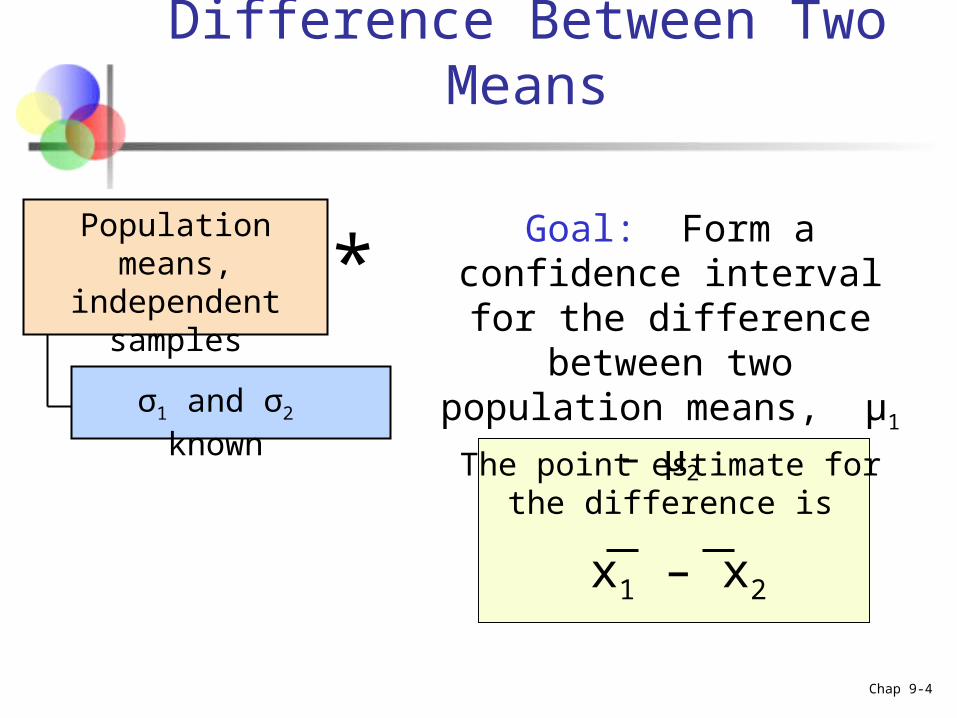
Difference Between Two Means
Population means, independent
samples
σ1 and σ2 known
Goal: Form a confidence interval for the difference between two population
means, μ1 – μ2
The point estimate for the difference is
x1 – x2
*
Chap 9-5
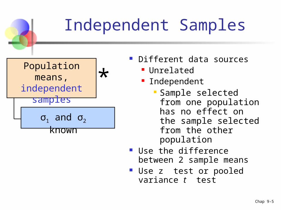
Independent Samples
Population means, independent
samples
σ1 and σ2 known
Different data sources Unrelated Independent
Sample selected from one population has no effect on the sample selected from the other population
Use the difference between 2 sample means
Use z test or pooled variance t test
*

Chap 9-6
Population means, independent
samples
σ1 and σ2 known
σ1 and σ2 known
Assumptions:
Samples are randomly and independently drawn
population distributions are normal or both sample sizes are 30
Population standard deviations are known
*

Chap 9-7
Population means, independent
samples
σ1 and σ2 known …and the standard error of
x1 – x2 is
When σ1 and σ2 are known and both populations are normal or both sample sizes are at least 30, the test statistic is a z-value…
2
22
1
21
xx n
σ
n
σσ
21
(continued)
σ1 and σ2 known
*

Chap 9-8
Population means, independent
samples
σ1 and σ2 known
2
22
1
21
/221n
σ
n
σzxx
The confidence interval for
μ1 – μ2 is:
σ1 and σ2 known(continued)
*

Chap 9-9
Population means, independent
samples
σ1 and σ2 known
σ1 and σ2 unknown,
σ1 and σ2 unknown
Assumptions:
populations are normally distributed
the populations have equal variances
samples are independent
*
Chap 9-10
Population means, independent
samples
σ1 and σ2 known
σ1 and σ2 unknown,
σ1 and σ2 unknown
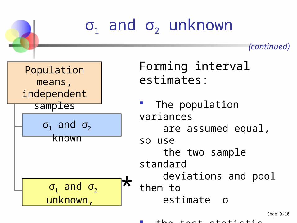
Forming interval estimates:
The population variances are assumed equal, so use the two sample standard deviations and pool them to estimate σ
the test statistic is a t value with (n1 + n2 – 2) degrees of freedom
(continued)
*
Chap 9-11
Population means, independent
samples
σ1 and σ2 known
σ1 and σ2 unknown
σ1 and σ2 unknown
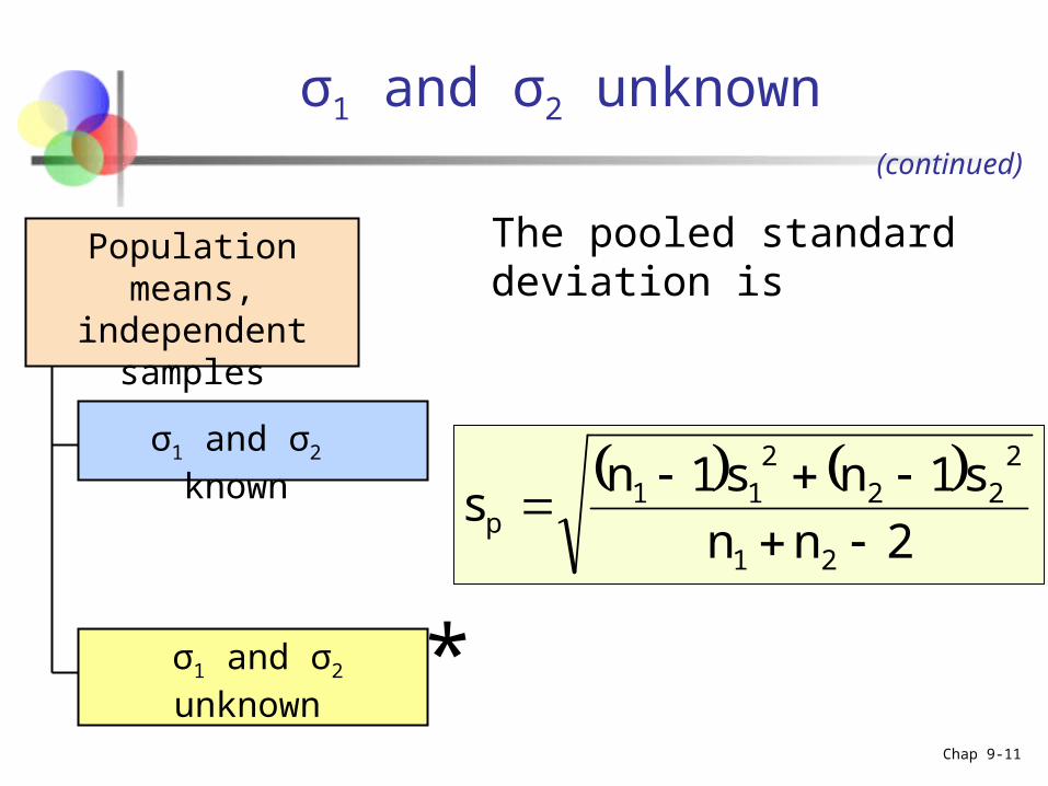
The pooled standard deviation is
(continued)
2nn
s1ns1ns
21
222
211
p
*
Chap 9-12
Population means, independent
samples
σ1 and σ2 known
σ1 and σ2 unknown
21
p/221n
1
n
1stxx
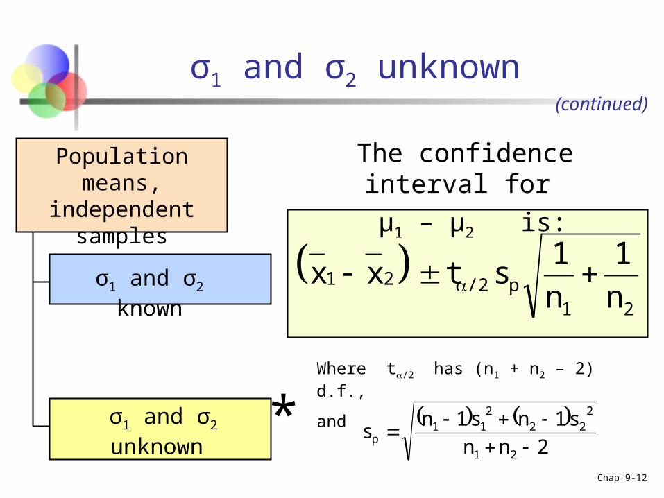
The confidence interval for
μ1 – μ2 is:
σ1 and σ2 unknown(continued)
Where t/2 has (n1 + n2 – 2) d.f.,
and
2nn
s1ns1ns
21
222
211
p
*

Chap 9-13
Paired Samples
Tests Means of 2 Related Populations Paired or matched samples Repeated measures (before/after) Use difference between paired values:
Eliminates Variation Among Subjects Assumptions:
Both Populations Are Normally Distributed Or, if Not Normal, use large samples
Paired samples
d = x1 - x2

Chap 9-14
Paired Differences
The ith paired difference is di , wherePaired
samplesdi = x1i - x2i
The point estimate for the population mean paired difference is d :
1n
)d(ds
n
1i
2i
d
n
dd
n
1ii
The sample standard deviation is
n is the number of pairs in the paired sample
Chap 9-15
Paired Differences
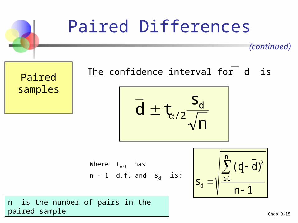
The confidence interval for d isPaired samples
1n
)d(ds
n
1i
2i
d
n
std d
/2
Where t/2 has
n - 1 d.f. and sd is:
(continued)
n is the number of pairs in the paired sample

Chap 9-16
Hypothesis Tests for the Difference Between Two Means
Testing Hypotheses about μ1 – μ2
Use the same situations discussed already:
Standard deviations known or unknown

Chap 9-17
Hypothesis Tests forTwo Population Proportions
Lower tail test:
H0: μ1 μ2
HA: μ1 < μ2
i.e.,
H0: μ1 – μ2 0HA: μ1 – μ2 < 0
Upper tail test:
H0: μ1 ≤ μ2
HA: μ1 > μ2
i.e.,
H0: μ1 – μ2 ≤ 0HA: μ1 – μ2 > 0
Two-tailed test:
H0: μ1 = μ2
HA: μ1 ≠ μ2
i.e.,
H0: μ1 – μ2 = 0HA: μ1 – μ2 ≠ 0
Two Population Means, Independent Samples

Chap 9-18
Hypothesis tests for μ1 – μ2
Population means, independent samples
σ1 and σ2 known
σ1 and σ2 unknown
Use a z test statistic
Use s to estimate unknown σ , use a t test statistic and pooled standard deviation
Chap 9-19
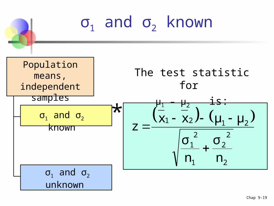
Population means, independent
samples
σ1 and σ2 known
σ1 and σ2 unknown
2
22
1
21
2121
nσ
nσ
μμxxz
The test statistic for
μ1 – μ2 is:
σ1 and σ2 known
*

Chap 9-20
Population means, independent
samples
σ1 and σ2 known
σ1 and σ2 unknown
σ1 and σ2 unknown
Where t/2 has (n1 + n2 – 2) d.f.,
and
2nn
s1ns1ns
21
222
211
p
21p
2121
n1
n1
s
μμxxt
The test statistic for
μ1 – μ2 is:
*

Chap 9-21
Two Population Means, Independent Samples
Lower tail test:
H0: μ1 – μ2 0HA: μ1 – μ2 < 0
Upper tail test:
H0: μ1 – μ2 ≤ 0HA: μ1 – μ2 > 0
Two-tailed test:
H0: μ1 – μ2 = 0HA: μ1 – μ2 ≠ 0
/2 /2
-z -z/2z z/2
Reject H0 if z < -z Reject H0 if z > z Reject H0 if z < -z/2
or z > z/2
Hypothesis tests for μ1 – μ2
Chap 9-22
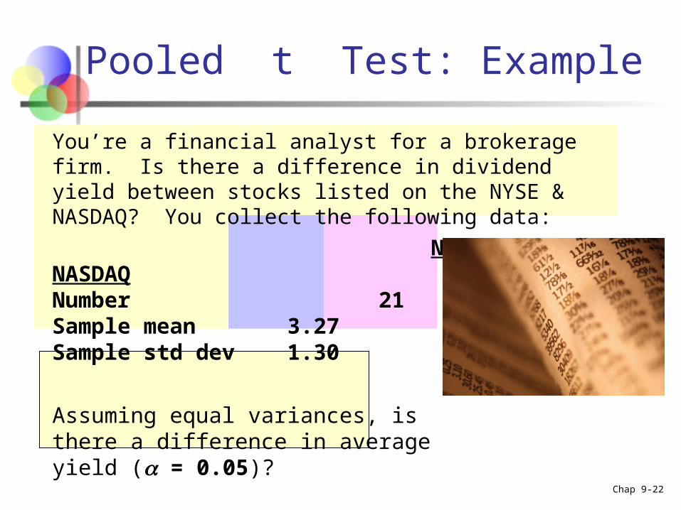
Pooled t Test: Example
You’re a financial analyst for a brokerage firm. Is there a difference in dividend yield between stocks listed on the NYSE & NASDAQ? You collect the following data:
NYSE NASDAQNumber 21 25Sample mean 3.27 2.53Sample std dev 1.30 1.16
Assuming equal variances, isthere a difference in average yield ( = 0.05)?

Chap 9-23
Calculating the Test Statistic
1.2256
22521
1.161251.30121
2nn
s1ns1ns
22
21
222
211
p
2.040
251
211
1.2256
02.533.27
n1
n1
s
μμxxt
21p
2121
The test statistic is:

Chap 9-24
Solution
H0: μ1 - μ2 = 0 i.e. (μ1 = μ2)
HA: μ1 - μ2 ≠ 0 i.e. (μ1 ≠ μ2)
= 0.05
df = 21 + 25 - 2 = 44Critical Values: t = ± 2.0154
Test Statistic: Decision:
Conclusion:
Reject H0 at = 0.05There is evidence of a difference in means.
t0 2.0154-2.0154
.025
Reject H0 Reject H0
.025
2.040
2.040
251
211
1.2256
2.533.27t

Chap 9-25
The test statistic for d isPaired
samples
1n
)d(ds
n
1i
2i
d
n
sμd
td
d
Where t/2 has n - 1 d.f.
and sd is:
n is the number of pairs in the paired sample
Hypothesis Testing for Paired Samples

Chap 9-26
Lower tail test:
H0: μd 0HA: μd < 0
Upper tail test:
H0: μd ≤ 0HA: μd > 0
Two-tailed test:
H0: μd = 0HA: μd ≠ 0
Paired Samples
Hypothesis Testing for Paired Samples
/2 /2
-t -t/2t t/2
Reject H0 if t < -t Reject H0 if t > t Reject H0 if t < -t
or t > t Where t has n - 1 d.f.
(continued)
Chap 9-27
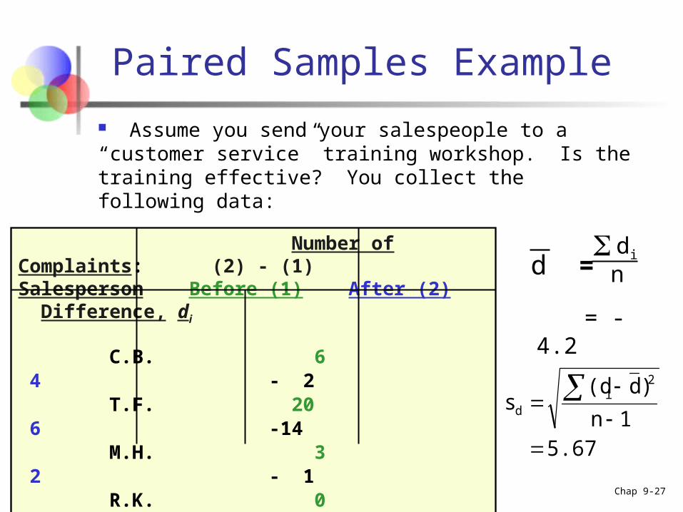
Assume you send your salespeople to a “customer service” training workshop. Is the training effective? You collect the following data:
Paired Samples Example
Number of Complaints: (2) - (1)Salesperson Before (1) After (2) Difference, di
C.B. 6 4 - 2 T.F. 20 6 -14 M.H. 3 2 - 1 R.K. 0 0 0 M.O. 4 0 - 4 -21
d = di
n
5.671n
)d(ds
2i
d
= -4.2

Chap 9-28
Has the training made a difference in the number of complaints (at the 0.01 level)?
- 4.2d =
1.6655.67/
04.2
n/s
μdt
d
d
H0: μd = 0HA: μd 0
Test Statistic:
Critical Value = ± 4.604 d.f. = n - 1 = 4
Reject
/2
- 4.604 4.604
Decision: Do not reject H0
(t stat is not in the reject region)
Conclusion: There is not a significant change in the number of complaints.
Paired Samples: Solution
Reject
/2
- 1.66 = .01

Chap 9-29
Two Population Proportions
Goal: Form a confidence interval for or test a hypothesis about the difference between two population proportions, p1 – p2
The point estimate for the difference is p1 – p2
Population proportions
Assumptions: n1p1 5 , n1(1-p1) 5
n2p2 5 , n2(1-p2) 5

Chap 9-30
Confidence Interval forTwo Population Proportions
Population proportions
2
22
1
11/221 n
)p(1p
n
)p(1pzpp
The confidence interval for
p1 – p2 is:

Chap 9-31
Hypothesis Tests forTwo Population Proportions
Population proportions
Lower tail test:
H0: p1 p2
HA: p1 < p2
i.e.,
H0: p1 – p2 0HA: p1 – p2 < 0
Upper tail test:
H0: p1 ≤ p2
HA: p1 > p2
i.e.,
H0: p1 – p2 ≤ 0HA: p1 – p2 > 0
Two-tailed test:
H0: p1 = p2
HA: p1 ≠ p2
i.e.,
H0: p1 – p2 = 0HA: p1 – p2 ≠ 0

Chap 9-32
Two Population Proportions
Population proportions
21
21
21
2211
nn
xx
nn
pnpnp
The pooled estimate for the overall proportion is:
where x1 and x2 are the numbers from
samples 1 and 2 with the characteristic of interest
Since we begin by assuming the null hypothesis is true, we assume p1 = p2
and pool the two p estimates

Chap 9-33
Two Population Proportions
Population proportions
21
2121
n1
n1
)p1(p
ppppz
The test statistic for
p1 – p2 is:
(continued)
Chap 9-34
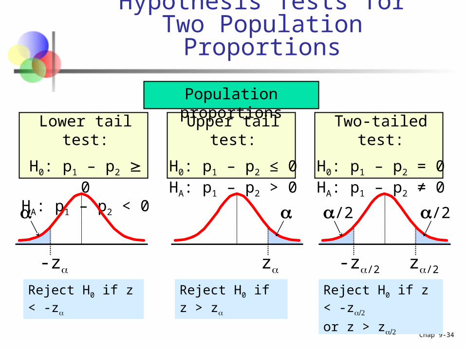
Hypothesis Tests forTwo Population Proportions
Population proportions
Lower tail test:
H0: p1 – p2 0HA: p1 – p2 < 0
Upper tail test:
H0: p1 – p2 ≤ 0HA: p1 – p2 > 0
Two-tailed test:
H0: p1 – p2 = 0HA: p1 – p2 ≠ 0
/2 /2
-z -z/2z z/2
Reject H0 if z < -z Reject H0 if z > z Reject H0 if z < -z
or z > z

Chap 9-35
Example: Two population Proportions
Is there a significant difference between the proportion of men and the proportion of women who will vote Yes on Proposition A?
In a random sample, 36 of 72 men and 31 of 50 women indicated they would vote Yes
Test at the .05 level of significance

Chap 9-36
The hypothesis test is:
H0: p1 – p2 = 0 (the two proportions are equal)
HA: p1 – p2 ≠ 0 (there is a significant difference between proportions)
The sample proportions are: Men: p1 = 36/72 = .50
Women: p2 = 31/50 = .62
.549122
67
5072
3136
nn
xxp
21
21
The pooled estimate for the overall proportion is:
Example: Two population Proportions
(continued)
Chap 9-37
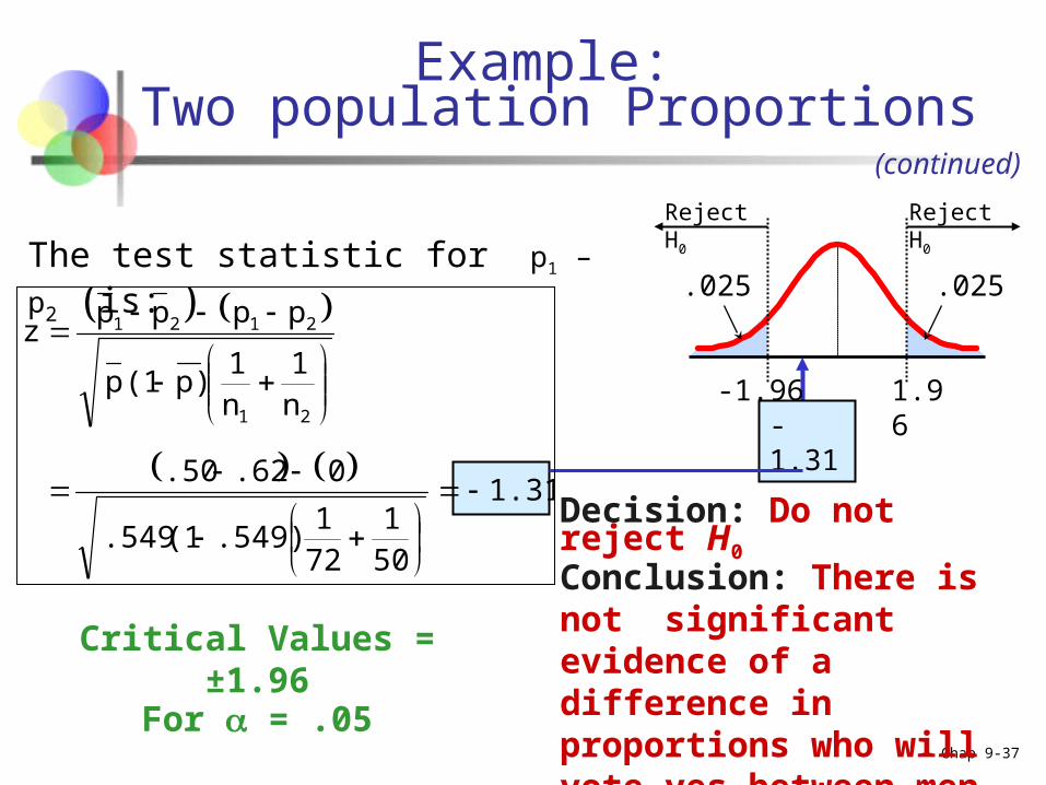
The test statistic for p1 – p2 is:
Example: Two population Proportions
(continued)
.025
-1.96 1.96
.025
-1.31
Decision: Do not reject H0
Conclusion: There is not significant evidence of a difference in proportions who will vote yes between men and women.
1.31
501
721
.549)(1.549
0.62.50
n1
n1
p)(1p
ppppz
21
2121
Reject H0 Reject H0
Critical Values = ±1.96For = .05

Chap 9-38
Two Sample Tests in EXCEL
For independent samples: Independent sample Z test with variances known:
Tools | data analysis | z-test: two sample for means
Independent sample Z test with large sample Tools | data analysis | z-test: two sample for means If the population variances are unknown, use sample variances
For paired samples (t test): Tools | data analysis… | t-test: paired two sample for means

Chap 9-39
Contingency Tables
Contingency Tables
Situations involving multiple population proportions
Used to classify sample observations according to two or more characteristics
Also called a crosstabulation table.
Chap 9-40
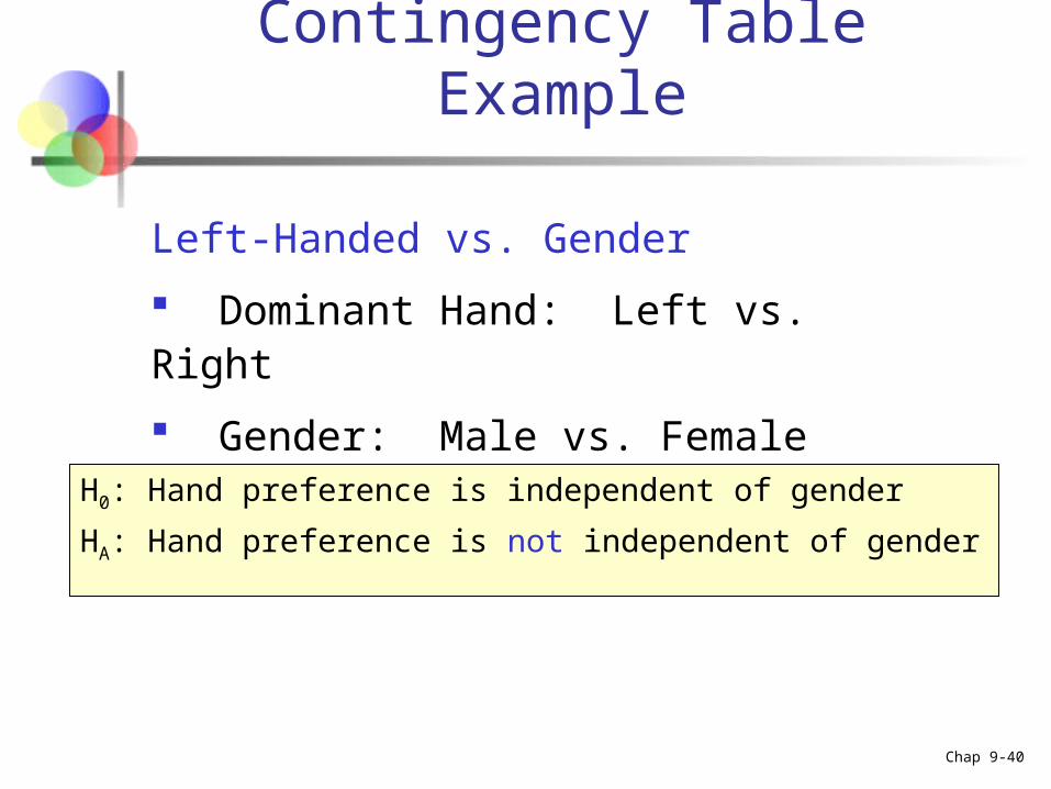
Contingency Table Example
H0: Hand preference is independent of gender
HA: Hand preference is not independent of gender
Left-Handed vs. Gender
Dominant Hand: Left vs. Right
Gender: Male vs. Female

Chap 9-41
Contingency Table Example
Sample results organized in a contingency table:
(continued)
Gender
Hand Preference
Left Right
Female 12 108 120
Male 24 156 180
36 264 300
120 Females, 12 were left handed
180 Males, 24 were left handed
sample size = n = 300:

Chap 9-42
Logic of the Test
If H0 is true, then the proportion of left-handed females should be the same as the proportion of left-handed males
The two proportions above should be the same as the proportion of left-handed people overall
H0: Hand preference is independent of gender
HA: Hand preference is not independent of gender

Chap 9-43
Finding Expected Frequencies
Overall:
P(Left Handed)
= 36/300 = .12
120 Females, 12 were left handed
180 Males, 24 were left handed
If independent, then
P(Left Handed | Female) = P(Left Handed | Male) = .12
So we would expect 12% of the 120 females and 12% of the 180 males to be left handed…
i.e., we would expect (120)(.12) = 14.4 females to be left handed(180)(.12) = 21.6 males to be left handed

Chap 9-44
Expected Cell Frequencies
Expected cell frequencies:(continued)
size sample Total
total) Column jtotal)(Row i(e
thth
ij
4.14300
)36)(120(e11
Example:
Chap 9-45
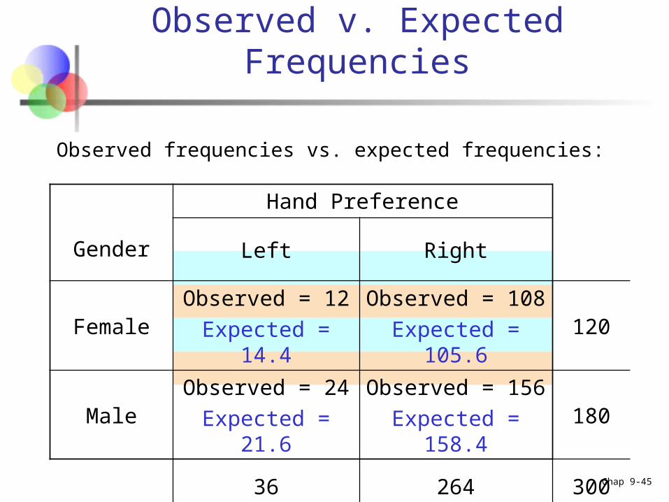
Observed v. Expected Frequencies
Observed frequencies vs. expected frequencies:
Gender
Hand Preference
Left Right
FemaleObserved = 12
Expected = 14.4
Observed = 108
Expected = 105.6120
MaleObserved = 24
Expected = 21.6
Observed = 156
Expected = 158.4180
36 264 300

Chap 9-46
The Chi-Square Test Statistic
where:
oij = observed frequency in cell (i, j)
eij = expected frequency in cell (i, j) r = number of rows c = number of columns
r
1i
c
1j ij
2ijij2
e
)eo(
The Chi-square contingency test statistic is:
)1c)(1r(.f.d with
Chap 9-47
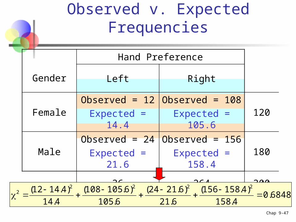
Observed v. Expected Frequencies
Gender
Hand Preference
Left Right
FemaleObserved = 12
Expected = 14.4
Observed = 108
Expected = 105.6120
MaleObserved = 24
Expected = 21.6
Observed = 156
Expected = 158.4180
36 264 300
6848.04.158
)4.158156(
6.21
)6.2124(
6.105
)6.105108(
4.14
)4.1412( 22222
Chap 9-48
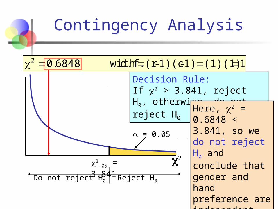
Contingency Analysis
2
.05 = 3.841
Reject H0
= 0.05
Decision Rule:If 2 > 3.841, reject H0, otherwise, do not reject H0
1(1)(1)1)-1)(c-(r d.f. with6848.02
Do not reject H0
Here, 2 = 0.6848 < 3.841, so we do not reject H0 and conclude that gender and hand preference are independent
Chap 9-49
Chapter Summary
Used the chi-square goodness-of-fit test to determine whether data fits a specified distribution Example of a discrete distribution (uniform) Example of a continuous distribution (normal)
Used contingency tables to perform a chi-square test of independence Compared observed cell frequencies to expected cell
frequencies
Chap 9-50
Chapter Summary Compared two independent samples
Formed confidence intervals for the differences between two means Performed Z test for the differences in two means Performed t test for the differences in two means
Compared two related samples (paired samples) Formed confidence intervals for the paired difference Performed paired sample t tests for the mean difference
Compared two population proportions Formed confidence intervals for the difference between two
population proportions Performed Z-test for two population proportions
Used contingency tables to perform a chi-square test of independence