Chap 3. Generation, Transformation and Deformation of Random Sea Waves

3.1 Simplified Forecasting Method of Wind Waves and Swell

Numerical model for directional wave spectrum: WAM or SWAN (including shallow

water effects) ← good for both tropical (e.g. typhoon) and extratropical storms

SMB method: Assume a constant wind speed U over a fixed fetch length F for a

certain duration t . Good for extratropical storms (e.g. Northwesters on the west coast

of Korea during winter) or wind wave generation in an enclosed basin.

Wilson’s formulas (Eqs. 3.1 and 3.2): Based on SMB method, but modified to be

applicable to tropical cyclones of large temporal and spatial variation of wind.

Fully-developed condition: both F and t are long enough

Fetch-limited condition: t is long enough, but F is limited

Duration-limited condition: F is long enough, but t is limited

Minimum duration for fetch-limited condition = mint ← Eqs. (3.3) or (3.4)

Minimum fetch length for fully-developed waves for given t = minF ← Eq. (3.5)

If mint t , fetch-limited → Use Eqs. (3.1) and (3.2)

If mint t , duration-limited → Calculate minF using Eq. (3.5). Then use Eqs. (3.1)

and (3.2) with minF F

Relationship between 1/3H and 1/3T : 0.631/3 1/33.3( )T H (3.6) ← good for large waves

comparable to design waves but gives lower limit of 1/3T for smaller waves (see Suh et

al. 2010, Coastal Engineering 57, 375-384)

Swell height and period: Eqs. (3.7) and (3.8) as a function of swell travel distance D

Relationship between wave height and period of wind waves and swell: Fig. 3.4

3.2 Wave Refraction (+Shoaling)

3.2.1 Introduction

Ray theory for regular waves

Conservation of energy:

0020

2

8

1

8

1bCgHbCgH gg

which gives

rs KKHH 0

shoaling coefficient, ),(2sinh

21tanh

2/1

0 hfKkh

khkh

C

CK s

g

gs

refraction coefficient, ),,(0 hfKb

bK rr ; ),,( 0 hf

3.2.2 Refraction Coefficient of Random Sea Waves

000

2 ),(),,(),(),( fShfKhfKfS rs

0

2

0002 ),,(),(),(),()(

dhfKfShfKdfSfS rs

0 02

000

0 02

00000

max

min

),,(),(),(

),,(),(),()(

dfdhfKhfKfS

dfdhfKhfKfSdffSm

rs

rs

Goda’s book uses

0 0

2000

max

min

),(),( dfdhfKfSm ss

Define 2/1

0

0

seffr m

mK

For example, 00 4 mHm = significant wave height after shoaling and refraction

00 4 sms mH = significant wave height due to shoaling only

then, 00 mseffrm HKH

In actual calculations, the integration is performed by a summation of frequency and

direction.

1/2

2

1 1

( ) ( )M N

r ij r ijeffi j

K E K

Goda’s book explains how to discretize f and .

area total)(00

dffSm

),,2,1()( 0~

~ MiM

mdffS

ii

i

ff

f

)( fS can be integrated analytically (e.g. B-M or P-M spectra), say

)exp()( 45 bfaffS

b

abf

b

adffSm

4)exp(

4)(

0

4

00

Similarly,

M

mfbffb

b

abf

b

adffS iii

ff

f

ff

f

ii

i

ii

i

044

~

~

4~

~ )~

exp(])~

(exp[4

)exp(4

)(

Hence,

),,2,1(1

)~

exp(])~

(exp[ 44 MiM

fbffb iii

Now we can find ),,2,1( Mifi starting from 0~

1 f .

Representative frequency if for the band ( if~

to ii ff ~

)?

Goda suggests on the basis of 20 / mmT and

0

22 )( dffSfm

i

ii m

mf

0

2

Mb

a

M

mm i

1

40

0

ii

i

ii

i

ff

f

ff

fi dfbfafdffSfm~

~43

~

~2

2 )exp()(

Putting b

ddfffb

22232

,

2

2

2

2

)~

(2

)~

(2

2)~

(2

)~

(2

22 )2/exp(

22)2/exp(

22

i

ii

ii

i

fb

ffb

ffb

fbi db

ad

b

am

Goda defines error function, t

dxxt0

2 )2/exp(2/1)( , though usual definition is

t

dxxterf0

2 )exp(/2)( so that 1)( erf . Thus,

22

2

~2

~2

2 iiii ffbfbb

am

2/1222/1

0

2 ~2

~22

iii

i

ii ffbfbMb

m

mf

which should correspond to Eq. (3.15) in Goda’s book if 403.1 sTb (B-M spectrum):

2/1

2/1 ln21

ln2)912.2(9.0

1

i

M

i

MM

Tf

si

It is required

),,2,1(~

21

ln22

Mifbi

Mi

On the other hand, M

fbffb iii

1~exp

~exp

44

Take 1

ln~ 4

i

Mfb i . Then

MM

i

M

i 11

satisfied.

As for the discretization of wave angle (16-point bearing, see Table 3.2),

3.2.3 Computation of Random Wave Refraction by Means of the Energy Balance

Equation

General transport equation for S (any scalar quantity):

QVSt

S

)( (sink or source of S )

where V = transport velocity of S . For ),,,,( fyxtS = directional random waves,

V = velocity following waves

fyx vvvvdt

df

dt

d

dt

dy

dt

dxV ,,,,,,

with

cosgx Cv , singy Cv

cossiny

C

x

C

C

Cv g to account for refraction

0fv assuming f does not change following the wave.

Then

QvfSvfSy

vfSxt

fSyx

),(),(),(),(

For steady state ( 0/ tS ) with no sink or source ( 0Q ),

0

SvSv

ySv

x yx for ),,,( fyxS

Assuming ),( yx , or x , y , are independent variables,

0cossinsincos

y

C

x

CSC

y

SCC

x

SCCg

gg

where C and gC using linear wave theory depend on ),( yxh and frequency f .

is computed by ray theory. We need boundary conditions for S .

Example in Goda’s book Fig. 3.7: Waves over a circular shoal

• sT as well as sH changes depending on locations (Fig. 3.8).

• Fig. 3.9 for regular waves shows larger spatial variations of wave heights.

Ref. Vincent and Briggs (1989). Refraction-diffraction of irregular waves over a mound,

JWPCOE, 115(2), 269-284: Performed laboratory experiments on transformation of

monochromatic and random directional waves over an elliptic shoal. They concluded

that monochromatic waves using representative wave height and period (e.g. sH and

sT ) provide a poor approximation of irregular wave conditions if there is directional

spread or high wave steepness.

Ref. Kweon, H.-M. (1998). A 3-D random breaking model for directional spectral

waves, Jpornal of the Korean Society of Civil Engineers, 18(II-6), 591-599 (in Korean):

Include sink term due to wave breaking.

Ref. Mase, H. (2001). Multi-directional random wave transformation model based on

energy balance equation, Coastal Engineering Journal, 43(4), 317-337: Include wave

diffraction.

3.2.4 Wave Refraction on a Coast with Straight, Parallel Depth Contours

Snell’s law: 0

0sinsin

CC

can find ),,( 0 hf

0

Refraction coefficient

cos

cos),,( 0

0 hfKr

Shoaling coefficient ),(0 hfKC

CK s

g

gs

Directional spectrum ),( fS in water depth h :

),(),,(),(),( 00

1

0

20

fShfKhfKfS rs

Need to specify ),( 00 fS in deep water. For example, ),()(),( 0000 fGfSfS

with )(0 fS = B-M spectrum with given 0ms HH and 05.1/ps TT ,

),( 0fG = Mitsuyasu-type with given maxs and 0p ,

0p = predominant wave direction in deep water,

00002

00 ;2

cos),( ppsGfG ,

0GG is maximum at 00 p .

Fig. 3.10 shows effrK given by Eq. (3.10) as a function of 0/ Lh with

2/20 sgTL ,

0p and maxs .

Note: 1effrK even for 00p ( directional spreading).

3.3 Wave Diffraction

3.3.1 Principle of Random Wave Diffraction Analysis

For linear monochromatic waves in constant water depth, Sommerfeld solution for a

semi-infinite thin breakwater:

Diffraction coefficient id HyxHK /),( depends on f , i , and h =constant.

),()(

),,;,(),(

ii

iid

fSfS

HhyxfKyxH

Frequency spectrum

iiiid dfSfKyxfS ),(),(),(given at )( 2

Since

0

2

00),(),(),()(

dfdfSfKdfdfSdffS iiiid

therefore

iiiid fSfKfS ),(),(),( 2

Then

iiiid dfSfKdfSfS ),(),(),()( 2

In terms of zeroth moment,

iimiiii mHdfdfSm 0000 4),(

: incident significant wave height

0000 4),( mHdfdfSm m

: significant wave height at ),( yx

0

20 ),(),(

dfdfSfKm iiiid

Define effective diffraction coefficient:

1/2

0 0

0 0

1/2

2

00

(3.22) in Goda's book where added

1( , ) ( , )

md eff

m i i

i i d i i

i

H mK i

H m

S f K f d dfm

Read Goda’s book for field measurement (Figs. 3.13 and 3.14). deffd KK based on

regular waves with 3/1HH and 3/1TT = 0.07, which is significantly

underestimated in this case.

3.3.2 Diffraction Diagrams of Random Sea Waves

iiiid dfShyxfKhyxfS ),(),,;,(),,;( 2

00 )(),,( dffShyxm ;

00 )( dffSm ii

0

22 )(),,( dffSfhyxm ;

0

22 )( dffSfm ii

peak ),,( hyxTp from )( fS ; peak ipT from )( fSi

2000 /,4 mmTmHm ; iiiiim mmTmH 2000 /,4

05.1/,0 psms TTHH ; 05.1/,0 ipisimis TTHH

Wave height ratio = is

s

im

meffd H

H

H

HK

0

0 only for sm HH 0

Period ratio iT

T or is

s

ip

p

T

T

T

T

It is not specified in Goda’s book which relation is used for period ratio. It is likely to

use iTT / since pT may be difficult to find. But Goda uses isT to find L (p.82).

Goda assumed ),()(),( iiii fGfSfS with B-M frequency spectrum and

Mitsuyasu-type directional spreading.

Need to specify imis HH 0 , 05.1/ipis TT , maxs ,

ip , constant depth h , and

breakwater geometry.

(probably) ratio period

ratioheight

Plotted

is

s

effd

T

TK

for normal incidence only, 0ip .

Fig. 3.15 for a semi-infinite breakwater, for 10max s (wind waves) and 75max s

(swell, more unidirectional).

Monochromatic versus directional random waves:

1) In general, monochromatic wave underestimates wave heights in sheltered area,

and overestimates in open area.

2) The wave height ratio along the boundary of the geometric shadow (or the

straight line from the tip of the breakwater to the wave direction) is 0.7 for

directional random waves, while it is 0.5 for monochromatic waves.

Figs. 3.16~3.19 for breakwater gap ( 8,4,2,1/ LB )

3.3.3 Random Wave Diffraction of Oblique Incidence

Construct your own computer program if exact solution is needed. Otherwise, use an

approximate method suggested in the book.

3.3.4 Approximate Estimation of Diffracted Height by the Angular Spreading Method

For large barriers (e.g. headlands and islands),

region dilluminatein 1

shadow geometricin 0roughly

d

d

K

K

Neglect wave refraction.

00 ),(

dfdfSm iiii

Assume 0iS for 2/ i .

0

2/

2/0 ),(

dfdfSm iiii

0

2/

2/

20 ),(),(

dfdfSfKm iiiid

2/for 0

2/for 1 Assume

1

1

id

id

K

K

Then

0 2/0

1

),(

dfdfSm iii

0

1 10

( ) cumulative relative energy from / 2 to

Eq. (2.28) or Fig. 2.15 (B-M spectrum Mitsuyasu spreading)

E

i

mP

m

2/11

2/1

0

0 )(E

ieffd P

m

mK

01 and 02 for this problem

0

2/

0 2/0

2

1

),(

),(

dfdfS

dfdfSm

iii

iii

)()2/()( 210

0 EEE

i

PPPm

m

textin the

)(1)(

2

2

2

1

210

02

dd

EE

ieffd

KK

PPm

mK

3.3.5 Applicability of Regular Wave Diffraction Diagrams

Only for very narrow directional spreading

3.4 Equivalent Deepwater Wave

In real situation,

Hydraulic model test in 2D wave flume,

In real situation, 0sfsrds HKKKKH

In 2D wave flume, '0HKH ss

Thus, 00 ' sfrd HKKKH

(unrefracted) equivalent deepwater wave height

For wave period, usually assumes 0ss TT error if diffraction is dominant.

3.5 Wave Shoaling

Linear wave shoaling coeff. L

h

C

C

H

HK

g

gs offunction

'0

0

(3.25)

For shoaling of normally-incident linear random waves,

)();();( 02 fShfKhfS s can write a computer program easily.

For shoaling of nonlinear monochromatic waves, use Shuto (1974) model (read text).

Or you can use Eq. (3.31) with 1/3H and 1/3T (see Ex. 3.7).

3.6 Wave Deformation Due to Random Breaking

3.6.1 Breaker Index of Regular Waves

Breaker index: 0

tan ,b b

b

H hf

h L

Goda’s empirical formula (1970) for regular waves:

4/3

0 0

1 exp 1.5 1 15 tan ; 0.17/

b b

b b

H hAA

h h L L

(3.32)

with 2/20 gTL , which somewhat over-predicts over a steep slope. Rattanapikiton

and Shibayama (2000) modified it to

4/3

0 0

1 exp 1.5 1 11tan ; 0.17/

b b

b b

H hAA

h h L L

(3.33)

3.6.2 Hydrodynamics of Surf Zone

Regular waves break at a fixed location, but random waves break in a wide zone of

variable water depth → surf zone

Incipient wave breaking of random waves:

incipient 4/3

0 0

( )0.12 1 exp 1.5 1 11tanbb

hH

L L

Define 1/3 peak( )h = water depth at which 1/3H becomes the maximum inside surf zone,

1/3 peak( )H = maximum value of 1/3H inside surf zone

1/3 peak( )h and 1/3 peak( )H can be calculated by Figs. 3.28 and 3.29 and Eqs. (3.35)-(3.38).

Incipient breaker index of random waves: 1/3 peak 1/3 peak( ) / ( )H h in Fig. 3.30

Distribution of individual wave heights inside surf zone (see Fig. 3.31):

- Rayleigh distribution in relatively deep water

- Enhancement of large waves due to nonlinear shoaling near breaking point →

longer right tail

- Breaking of large waves inside surf zone → upper tail truncated

- Regeneration of nonbreaking waves in much shallow area near shoreline →

widening toward Rayleigh distribution (not shown in Fig. 3.31)

- Upper curves of Fig. 3.32 (lab, 2% 1/3/ 1.4H H for Rayleigh) and Fig. 3.33

(field, 1/10 1/3/ 1.27H H for Rayleigh) prove these changes.

Water level change:

Wave setup ( ) was computed using the results of monochromatic waves with sT and

2H = mean square of random waves, the latter of which is affected by . Therefore,

we need iteration to solve and 2H simultaneously. See Eq. (3.40) and Fig. 3.34.

(= at 0z ) = wave setup at still-water shoreline: Eq. (3.41) and Fig. 3.35

s (maximum ) = maximum wave setup on swash zone: Eq. (3.45)

Surf beat, )(t : slow (30~300 s) fluctuation of free surface mainly inside surf zone

from Gaussian distribution with rms given by Eq. (3.46)

Thus, )(tdh

3.6.3 Wave Height Variations on Planar Beaches

Before wave breaking, Rayleigh distribution may be assumed

H

Hxxxxp

;

4exp

2)( 2

0

(2.1)

After breaking, )()(0 xpxp

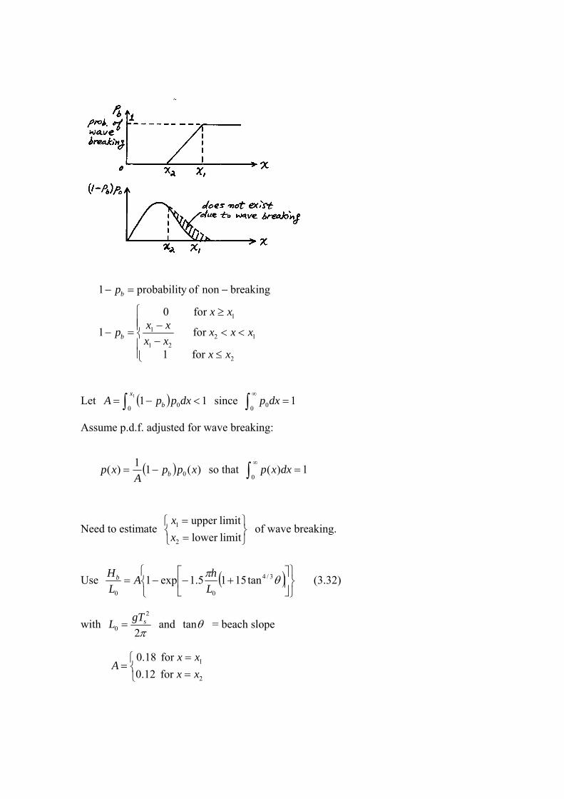
breakingnon ofy probabilit1 bp

2

1221

1

1

for 1

for

for 0

1

xx

xxxxx

xxxx

pb

Let 111

0 0 x

b dxppA since 10 0

dxp

Assume p.d.f. adjusted for wave breaking:

)(11

)( 0 xppA

xp b so that 1)(0

dxxp

Need to estimate

limitlower

limitupper

2

1

x

x of wave breaking.

Use

3/4

00

tan1515.1exp1L

hA

L

Hb (3.32)

with 2

2

0sgT

L and tan = beach slope

2

1

for 12.0

for 18.0

xx

xxA

Eq. (3.32) was developed for breaking point ( bhh ) of regular waves. But it may be

used inside the surf zone if bH = broken wave height, h = local depth.

Verification of the model with laboratory (Fig. 3.37) and field (Fig. 3.38) data

Diagrams (Figs. 3.39 – 3.42) and formulas (Eqs. 3.47 – 3.48 and Table 3.6)

Improved and extended ( 1/3H and maxH → H , rmsH , 0mH , 1/3H , 1/10H and maxH )

equations are given by Rattanapitikon and Shibayama (2013, Coastal Engineering

Journal 55(3), 1350009-1~1350009-23)

3.7 Reflection of Waves and Their Propagation and Dissipation

3.7.1 Coefficient of Wave Reflection

RR

I

HK

H

Typical reflection coefficients are given in Table 3.8.

Reflection coefficient for sloping structure can be calculated by Eq. (3.50).

For perforated wall caissons, RK becomes minimum (0.3~0.4) at 2.0~15.0/ LB

(see Fig. 3.44). Under a standing wave system, maximum u at node maximum

energy dissipation & minimum reflection at 4/LB 25.0/ LB . However, in

reality, minimum reflection occurs at 2.0~15.0/ LB , due to inertia effect.

3.7.2 Propagation of Reflected Waves

ri (geometrical optics theory)

diamond pattern of surface profile

For long-period waves incident at large angle, Mach stem is formed.

amplitude dispersion

(Higher waves go faster.)

Reflection from finite length of seawall diffraction by breakwater gap

Reflection from very long seawall diffraction by semi-infinite breakwater

(or angular spreading method for headland)

Effect of opposing wind (sea land): attenuates waves of large steepness, but its effect

is minor for swell of low steepness.

3.7.3 Superposition of Incident and Reflected Waves

For linear waves, we can superpose the free surface displacement:

N

n

nRi yxtyxtyxt

1

),,(),,(),,(

total incident reflected waves

Time-averaged energy per unit surface area:

02 ),(given at gmyxg ;

00 )( dffSm

If the distance from the reflective structure is more than one wavelength, we may

assume

)(0),,,2,1(0 mnNn mR

nR

nRi uncorrelated.

Then

N

n

nRi

1

222

N

n

n

Ri S(f)mmmm1

0000 spectrumunder area ofaddition

N

n

n

Rmimm HHH1

2

02

02

0 (3.51)

Fig. 3.48 indicates 202

00 Rmimm HHH at / 0.7x L

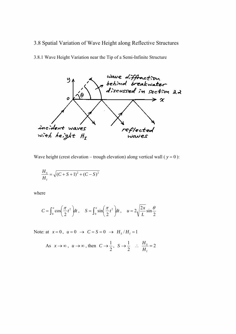
3.8 Spatial Variation of Wave Height along Reflective Structures

3.8.1 Wave Height Variation near the Tip of a Semi-Infinite Structure

Wave height (crest elevation – trough elevation) along vertical wall ( 0y ):

22 )()1( SCSCH

H

I

S

where

udttC

0

2

2cos

,

udttS

0

2

2sin

,

2sin

22

L

xu

Note: at 0x , 0u 0 SC 1/ IS HH

As x , u , then 2

1C ,

2

1S 2

I

S

H

H

less undulation

for irregular waves

For irregular waves, ( )d effK was calculated by Eq. (3.22) with I

Sd H

HK

for component waves

( uLf )

Explains meandering damage of concrete caissons.

3.8.2 Wave Height Variation at an Inward Corner of Reflective Structures

2

I

S

H

H (3.54)

for 2, I

S

H

H

4,2

I

S

H

H

wave height SH = crest elevation – trough elevation

Same as sum of 4 waves

propagating in 4 different directions

If the length is finite, use a computer program or an approximate method given in

Goda’s book.

3.8.3 Wave Height Variation along an Island Breakwater

cause undulation along wall (Fig. 3.54 and 3.55)

If LB , may add two waves diffracted from each tip:

3.9 Wave Transmission at Breakwaters and Low-Crested Structures

3.9.1 Wave Transmission Coefficient of Composite Breakwaters

transmission coefficient I

TT H

HK

Wave transmission through rubble mound may be negligible.

Expect

,material mound,,,,function TB

h

d

H

hK

I

cT

Fig. 3.56 for regular wave tests may be applicable to irregular waves with II HH 3/1 and TT HH 3/1 (see Fig. 3.57)

Eq. (3.57) function onlycT

si

hK

H

; Effect of

h

d is minor (see Fig. 3.56)

Eq. (3.58) horizontally composite breakwaters

1/3 1/3( ) / ( ) 1.2 0.28T I TT T K

3.9.2 Wave Transmission Coefficient of Low-Crested Structures (LCS)

Low-crested breakwater is built mostly for protection of sandy beaches

Wave transmission through LCS constructed with energy dissipating blocks: Fig. 3.58

(Tetrapods), Eq. (3.59)

Wave transmission over LCS: Eqs. (3.60)-(3.62)

Overall (through+over) transmission of LCS: Eq. (3.63)

3.9.3 Propagation of Transmitted Waves in a Harbor

No reliable information is available (Read text)