Embed Size (px)
Citation preview
KAUNAS UNIVERSITY OF TECHNOLOGY
RITA PALIVONAITĖ
CHAOTIC VISUAL CRYPTOGRAPHY
Doctoral Dissertation
Physical Sciences, Informatics (09P)
2015, KAUNAS

The research was accomplished during the period of 2010 – 2014 at Kaunas
University of Technology, Department of Mathematical Modelling. It was supported
by Research Council of Lithuania.
Scientific supervisor:
Prof. Dr. Habil. Minvydas Kazys Ragulskis (Kaunas University of
Technology, Physical Sciences, Informatics – 09P).
© R. Palivonaitė
2015
KAUNO TECHNOLOGIJOS UNIVERSITETAS
RITA PALIVONAITĖ
CHAOTINĖ VIZUALINĖ KRIPTOGRAFIJA
Daktaro disertacija
Fiziniai mokslai, informatika (09P)
2015, KAUNAS

Disertacija rengta 2010 – 2014 metais Kauno technologijos universitete,
Matematinio modeliavimo katedroje, remiant Lietuvos mokslo tarybai.
Mokslinis vadovas:
Prof. habil. dr. Minvydas Kazys Ragulskis (Kauno technologijos universitetas,
fiziniai mokslai, informatika – 09P).
© R. Palivonaitė
2015
5
Contents
NOMENCLATURE ................................................................................................... 8
INTRODUCTION .................................................................................................... 11
1. LITERATURE REVIEW ................................................................................. 15
1.1. Visual cryptography ...................................................................................... 15
1.1.1. Moiré techniques and applications ......................................................... 15
1.1.2. Classical visual cryptography and advanced modifications ................... 19
1.1.3. Visual cryptography based on moiré techniques .................................... 22
1.1.4. Dynamic visual cryptography based on time-averaged fringes produced
by harmonic oscillations ................................................................................... 24
1.1.5. Image hiding based on time-averaged fringes produced by non-harmonic
oscillations ........................................................................................................ 27
1.2. Time series segmentation algorithms ............................................................ 28
1.3. Time series forecasting models and algorithms ............................................. 33
1.3.1. Model-based time series forecasting methods ........................................ 34
1.3.2. Forecasting based on algebraic methods ................................................ 37
1.3.3. Forecasting based on smoothing methods .............................................. 38
1.3.4. Forecasting based on artificial neural networks (ANN) ......................... 39
1.3.5. Combined and hybrid methods for short-term time series forecasting ... 41
1.3.6. Metrics to measure forecasting accuracy ................................................ 43
1.4. Evolutionary algorithms ................................................................................ 44
1.4.1. Genetic algorithms .................................................................................. 44
1.4.2. Particle swarm optimization algorithm ................................................... 45
1.5. Quality and security aspects of visual cryptography schemes ....................... 47
1.6. Concluding remarks ....................................................................................... 51
2. ADVANCED DYNAMIC VISUAL CRYPTOGRAPHY ................................... 52
2.1. Image hiding based on near-optimal moiré gratings ..................................... 52
2.1.1. Initial definitions and optical background .............................................. 53
2.1.2. The construction of the optimality criterion for xF nm, .......................... 57
2.1.3. Perfect grayscale grating functions ......................................................... 59
2.1.4. The construction of evolutionary algorithms .......................................... 61
6
2.1.5. Image hiding in near optimal perfect grayscale gratings ........................ 65
2.1.6. Concluding remarks on near-optimal moiré gratings ............................. 71
2.2. Image hiding in time-averaged deformable moiré gratings ........................... 72
2.2.1. A non-deformable moiré grating with a constant pitch. ......................... 72
2.2.2. A deformable moiré grating with a constant pitch ................................. 73
2.2.3. A deformable moiré grating with a variable pitch .................................. 75
2.2.4. A deformable moiré grating with a step-incremental pitch .................... 76
2.2.5 Dynamic visual cryptography based on a variable pitch deformable moiré
grating ............................................................................................................... 78
2.2.6. Concluding remarks on deformable moiré gratings ............................... 83
2.3. Concluding remarks ....................................................................................... 84
3. CHAOTIC VISUAL CRYPTOGRAPHY ............................................................ 85
3.1. Image hiding based on chaotic oscillations ................................................... 85
3.1.1. Optical background and theoretical relationship .................................... 85
3.1.2. Computational representation of chaotic oscillations ............................. 87
3.1.3. Considerations about the size of a pixel ................................................. 88
3.1.4. Considerations about the standard deviation ..................................... 89
3.1.5. Simulation of chaotic oscillations on a computer screen ........................ 90
3.1.6. Visual decryption of the secret image .................................................... 91
3.1.7. Computational experiments .................................................................... 92
3.1.8. Concluding remarks ................................................................................ 95
3.2. Near-optimal moiré grating for chaotic dynamic visual cryptography .......... 96
3.2.1. Optical background and construction of the grayscale function ............. 96
3.2.2. Computational experiments .................................................................... 99
3.3. Concluding remarks on chaotic visual cryptography .................................. 100
3.4.The construction of the algebraic segmentation algorithm ........................... 102
3.4.1. The time series predictor based on skeleton sequences ........................ 102
3.4.2. The artificial time series ....................................................................... 103
3.4.3. One-step forward algebraic prediction of time series ........................... 105
3.4.4. Combinatorial aspects of the segmentation algorithm .......................... 107
3.4.5. The strategy for the selection of ........................................................ 109
7
3.4.6. Computational experiments with real-world time series ...................... 111
3.4.7. Comparisons with other segmentation techniques................................ 112
3.4.8. Concluding remarks .............................................................................. 115
3.5. The construction of the algebraic forecasting algorithm ............................. 116
3.5.1. One-step forward algebraic prediction of time series ........................... 116
3.5.2. The proposed scheme ........................................................................... 117
3.5.3. Effects of the additive noise ................................................................. 118
3.5.4. A simple numerical example ................................................................ 121
3.5.5. Parameter selection in PSO .................................................................. 121
3.5.6. The test time series with uniform noise ................................................ 124
3.5.7. Computational experiments on real-world time series ......................... 127
3.5.8. Concluding remarks .............................................................................. 131
CONCLUSIONS .................................................................................................... 132
REFERENCES ....................................................................................................... 133
LIST OF PUBLICATIONS .................................................................................... 151
Papers in Master List Journals of Institute of Scientific Information (ISI) ............ 151
Papers in Journals Reffered in the Databases, Included in the List Approved by the
Science Council of Lithuania ................................................................................. 151
Papers in Other Reviewed Scientific Editions ........................................................ 152
Papers in Proceedings List .............................................................................. 152

8
NOMENCLATURE
Literature review
a – the constant amplitude of harmonic oscillations;
ia and ib – Fourier coefficients;
AIC – Akaike information criterion;
te – the forecast error;
F – a stepped moiré grating function with pitch ; nH – the Hankel matrix (the catelecticant matrix with constant skew diagonals) ; n
is the order of the square matrix;
ss FH ;ˆ – time-averaging operator;
dI – d-th order of homogenous nonstationary process;
0J – the zero order Bessel function of the first kind;
L – the lag operator mtt
m xxL ;
yxM , – the grayscale level of the surface at point yx, ;
yM – the grayscale level of the surface at point y ;
m – the H-rank of the sequence 0; Zkxk ;
MAE – average of absolute forecasting errors; MAPE – average of percentage absolute
forecasting error; ME – average of forecasting errors; MSE – average of squared
forecasting errors;
2;0 N – Gaussian distribution;
jip ,– the grayscale level of an appropriate image based on two images (i and j)
geometric or algebraic superposition;
PSO – particle swarm optimization method;
q – the order of moving average MA(q) model;
ir – the i-th root of the zero order Bessel function of the first kind;
RMSE – root of average of squared forecasting errors;
ksssS ,,, 21 – k segmentation S is a partition of n,,2,1 into k not-overlapping
intervals or segments such that 11,, ibibi tts , where ib is the beginning of the
i-th segment;
is – the amplitude of oscillation at the center of the i-th fringe;
xSig – the sigmoid function;
SES – simple exponential smoothing;
SIC – Schwarz information criterion;
T – the exposure time;
ntttT ,,, 21 – time series sequence T consisting of n observations, Rti .
xu – the amplitude of harmonic oscillations;
9
iDiii vvvV ,,, 21 – particle’s speed in D-dimensional space;
– the cyclic frequency;
jiw , , jw – connection weights (artificial neural network (ANN) model parameters);
pi ,,2,1,0 , qj ,,2,1,0 ; p is the number of input nodes; and q is the number of
hidden nodes;
iDiii xxxX ,,, 21 – particle’s coordinates in D-dimensional space;
tx – the value of process (of the time series) at time t;
tx – moving average process;
tx – the first difference of the process at time t.
Greek symbols – smoothing factor ( 10 );
0 , 1 – coefficients of autoregressive process AR(1);
– deterministic trend coefficient;
}{ i – uncorrelated random shocks with zero mean and constant variance;
q
i
i
i LL0
– linear combination of lagged MA(q) process coefficients;
i – moving average MA(q) model coefficients;
– the pitch of the moiré grating;
– the mean of the process tx ;
s – a triangular waveform time function with oscillation amplitude s;
k – characteristic roots of the Hankel matrix, rk ,,2,1 ;
2 – the variance of the process tx ;
i – AR(p) model coefficients;
p
i
i
i LL0
– linear combination of lagged AR(p) process coefficients;
}{ i – the World decomposition coefficients, that satisfies inequality .1
2
i
i
Advanced and chaotic visual cryptography
ka , kb – Fourier coefficients;
A – the amplitude of harmonic oscillations of deformable moiré grating;
C , C – the infimum and the supremum of the grayscale grating function;
E – the averaging operator;
dE – the envelope function modulating the stationary grating;
xF – grayscale grating function;
xF~
– harmonic grating function;

10
xF – stepped grating function;
txFd , – the deformed moiré grating;
xF nm, – m-pixels of n-grayscale levels grating function;
xF – the norm of the grayscale grating function;
sH – time averaging operator;
0J – zero order Bessel function of the first kind;
kL – the coefficient of linearly increasing pitch moiré grating;
xps – the density function of the time function ts ;
P – the Fourier transform of the density function xp ;
P~
– the envelope function in chaotic visual cryptography;
nr – the n-th root of the zero order Bessel function of the first kind;
ky – grayscale levels of grayscale grating function xF nm, ;
Greek symbols
– the average of the grayscale grating function;
– the optimality criterion for a grayscale grating function;
– size of a pixel in digital screen;
– the crossover coefficient in genetic algorithms;
– the pitch of the grating;
– the crossover coefficient in genetic algorithms;
ts – time function, describing dynamic deflection from the state of equilibrium;
ts~
– time function, describing harmonic oscillations process;
ts – time function, describing triangular waveform type oscillation process;
– the standard deviation of a grayscale grating function;
jt – discrete normally distributed numbers at time t;
nmF , – the fitness function of a perfect grayscale grating function;
Short-term time series segmentation and forecasting
a – coefficient determining the penalty proportion;
mF 210 ,,, – the fitness function; k – the additive noise;
Hr – the H-rank of the sequence;
I – the identity matrix;
s – the averaging window in moving averaging algorithm;
kx~ – the sequence described by an algebraic progression;
– the prediction error level;
i – the penalty coefficient;
A – the spectrum of a square matrix A.
11
INTRODUCTION
Visual cryptography is a cryptographic technique which allows visual
information to be encrypted in such a way that the decryption can be performed by
the human visual system, without any cryptographic computation. Naor and Shamir
introduced this concept in 1994. They demonstrated a visual secret sharing scheme,
where the image was split up to n transparent shares so that only someone with all n
superimposed shares could decrypt the image, while any 1n shares revealed no
information about the original image. Since 1994 many advantages in visual
cryptography have been done, but all these schemes are based on the concept of image
splitting into n separate shares – until dynamic visual cryptography scheme (based on
geometric time-averaged moiré) was proposed in 2009.
Geometric moiré is a classical in-plane whole-field nondestructive optical
experimental technique based on analysis of visual patterns produced by superposition
of two regular gratings that geometrically interfere. The importance of the geometric
moiré phenomenon is demonstrated by its vast number of applications in many
different fields of industry, civil engineering, medical research, etc. Dynamic visual
cryptography is an alternative image hiding method that is based not on the static
superposition of shares (or geometric moiré images), but on time-averaging geometric
moiré. This method generates only one picture, and the secret image can be interpreted
by human visual system only when the original encoded image is harmonically
oscillated in a predefined direction at strictly defined amplitude of oscillation. If one
knows that the secret image appears while harmonically oscillated, trial and error
method can reveal secret image. Additional security measures are implemented,
where the secret image can be interpreted by a naked eye only when the time function
describing the oscillation of the encoded image is a triangular waveform.
Experimental implementations of dynamic visual cryptography require
generation of harmonic oscillations – the secret image is leaked in a form of moiré
fringes in the time-averaged image. Unfortunately, experimental generation of the
harmonic motion is not a straightforward task. A nonlinear system excited by
harmonic oscillations could result into a chaotic response. Therefore, the concept of
chaotic dynamic visual cryptography is an important problem both from the
theoretical and practical points of view. The ability to construct image hiding
cryptography scheme based on chaotic oscillations can be exploited in different
vibration related applications.
The feasibility of chaotic dynamic visual cryptography is one of the main topics
discussed in this dissertation. Theoretical relationships and computational
experiments are derived and discussed in details, though real-world experiments
remain a complicated task – simply because the human eye cannot perform averaging
in time with long expose times – the eye can capture an averaged image usually only
not longer than a split of a second. Therefore a tool for short-term time series
segmentation is a necessity for an effective experimental implementation of chaotic
dynamic visual cryptography.
Time series segmentation is a general data mining technique for summarizing
and analyzing sequential data. It gives a simplified representation of data and helps

12
the human eye to catch an overall picture of data. A proper segmentation of time series
provides a useful portrait of the local properties for the investigating and modelling
non-stationary systems. There are plenty time series segmentation methods based on
statistical information analysis. The prime requirements of these methods are based
on necessity to have long data sets, though acquiring long data sets is not usually
possible. The question of whether it is still possible to understand the complete
dynamics of a system if only short time series are observed is raised and analyzed. A
new segmentation technique based on the concept of skeleton algebraic sequences is
presented in this dissertation. This technique not only detects the moment of potential
change in evolution of the process. It also classifies skeleton sequences into separate
classes. This segmentation technique is based on evaluation of short-term time series
forecasting errors. Time series forecasting is an important task in many fields of
science and engineering. There are plenty forecasting methods that require long data,
but short-term time series analysis remains an important field of research. The concept
of skeleton algebraic sequences has been introduced in 2011 and has successfully
exploited for the prediction of short real-world time series. An improved algorithm
with internal smoothing procedure for short time series prediction is presented in this
dissertation. This procedure enabled to reach a healthy balance between excellent
variability of skeleton algebraic sequences and valuable properties of predictors based
the moving average method.
Object of the research: 1. Analytic relationships and modelling algorithms for the construction and
analysis of chaotic dynamic visual cryptography and image hiding
techniques based on moiré interference effects.
2. Chaotic dynamic visual cryptography realizations based on stationary
chaotic processes.
3. Segmentation models of chaotic processes based on the assessment of short-
term time series forecasting errors.
The aims of the research: 1. To construct, analyze and apply mathematical models and new algorithms
for the construction and analysis of the chaotic dynamic visual cryptography
and new image hiding techniques.
2. To construct and analyze mathematical models in order to identify the
models of time series dynamics and to apply these models for the
segmentation and forecasting of short-term time series.
To achieve these aims, the following tasks are solved in the dissertation:
1. To construct an improved dynamic visual cryptography scheme with
enhanced security based on near-optimal moiré grating, when the time
function determining the process of oscillation is periodic and comply with
specific requirements for the image hiding process.
2. To construct dynamic visual cryptography scheme based on the
deformations of the cover image according to a predetermined periodic law
of motion.
13
3. To construct and implement chaotic visual cryptography scheme which
visualizes the secret image only when the time function determining the
process of oscillation is chaotic.
4. To construct and implement an improved security chaotic visual
cryptography technique based on near-optimal moiré grating.
5. To construct a short-term time series segmentation methodology based on
short-term time series forecasting errors.
6. To construct a short-term time series forecasting technique based on the
variability of Hankel transformation and properties of skeleton algebraic
sequences.
Methods and software of the research:
Construction of the models of the investigated systems is based on mathematical
and statistical analysis as well as on the known facts of optical experimental geometric
and time-averaging moiré and further development of the moiré theory.
The methods and algorithms of construction and visualization of chaotic
dynamic visual cryptography are based on mathematical and statistical analysis,
numerical methods, principles of operators’ calculus and principles of digital images
processing.
The methods of mathematical, geometrical, statistical and algebraic analysis
theory are used in the research. Practical adoption of algebraic analysis is performed.
Programming tools used for research are Matlab2010b and standard toolboxes
(Image processing Toolbox, Image Acquisition Toolbox, Statistics Toolbox, and
Econometrics Toolbox), statistical packet SPSS v.16.
Programming tools created by the author. Classical recommendations are taken
into account for programming soft computing algorithms.
Scientific novelty and practical significance of the research:
1. A novel strategy for the construction of the optical moiré grating is
developed: genetic algorithms are used for the selection of a near-optimal
grating and a periodic law of motion which is employed for the decoding of
the secret image.
2. A new deformable dynamic visual cryptography technique based on the
deformation of cover images is developed. This scheme could be
implemented for the fault identification and control in micro-opto-
mechanical systems, where a stochastic cover moiré image could be formed
on the surface of movable components.
3. A chaotic dynamic visual cryptography scheme is developed. The secret
image is decoded if the cover image is oscillated according to a chaotic law.
This scheme can be exploited for visual monitoring of chaotic oscillations.
4. A novel short-term time series segmentation algorithm based on the
forecasting errors is developed. The combinatorial algorithm for the
identification of stationary segments and based on the forecasting error
levels is constructed. The developed algorithm can be used to identify the
segments of short-term time series – when the application of statistical
information about the evolution of the process is simply impossible due to
the lack of the available data.

14
5. An improved short-term time series forecasting technique for the
identification of pseudo-ranks of the sequence is developed. The practical
importance of the model is based on its ability to forecast short-term time
series contaminated by noise.
Author presents for the defense:
1. Novel modifications of dynamical visual cryptography for near optimal
moiré gratings.
2. Novel dynamic visual cryptography scheme based on deformable moiré
gratings.
3. Novel modifications of dynamical visual cryptography when the encoded
image can be decoded if the cover image does perform chaotic oscillations
with predefined parameters.
4. Novel short-term time series segmentation algorithm based on algebraic
relationships.
5. Novel modification of short-term time series forecasting technique based on
internal smoothing.
Approbation of the research:
11 scientific papers have been published on the subject of the dissertation,
including 7 papers listed in the ISI database with the citation index, other papers are
presented in the international conferences and the exhibition “KTU Technorama
2014” (presentation “The application of dynamic visual cryptography for human
visual system research” has won the third place).
The structure and volume of the dissertation:
Doctoral dissertation consists of an introduction, 3 main chapters, conclusions,
references, list of publications. Doctoral dissertation consists of 152 pages. The main
part of the dissertation contains 73 figures, 3 tables, and 250 entries in the reference
list.
15
1. LITERATURE REVIEW
1.1. Visual cryptography
1.1.1. Moiré techniques and applications
Geometric moiré is a classical in-plane whole field optical non-destructive
experimental technique based on examination of visual patterns produced by
superposition of two regular gratings that geometrically interfere [1, 2]. Equal-spaced
parallel lines, arrays of dots, concentric circles, etc. are typical examples of moiré
gratings. The gratings typically are superposed by direct contact, by reflection, by
shadowing, or by double-exposure photography [3, 4]. Moiré patterns are used to
measure variables such as displacements, rotations, curvature, and strains throughout
the viewed area.
One of the most important tasks in moiré pattern analysis is the analysis of the
distribution of moiré fringes. The research includes interpretation of experimentally
produced fringes patterns and determination of appropriate moiré fringes
displacements at centerlines. Moiré fringes in a pattern can be identified using manual,
semi-manual or fully automatic computational techniques [1]. Moiré pattern synthesis
requires the generation of a predefined moiré pattern. The synthesis process involves
the production of such two images that the required moiré pattern appears when those
images are superimposed [5].
The term moiré comes from French, where it refers to watered silk. The moiré
silk consists of two layers of fabric pressed together. If the silk is bent and folded, the
two layers move with respect to each other, causing the appearance of interfering
patterns [1]. Lord Rayleigh was the first who used the moiré for reduced sensitivity
testing by looking at the moiré between two identical gratings to determine their
quality [6].
The most common use of moiré, that is to determine strains and displacements
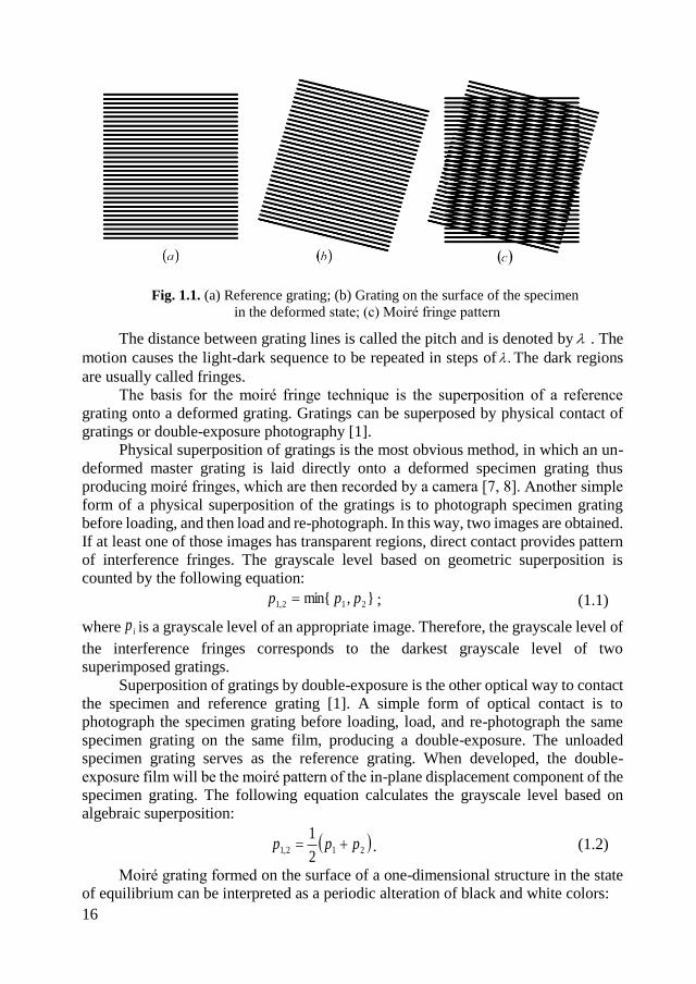
that act in and parallel to the plane of analysis, is presented in this chapter. In-plane
moiré is typically conducted with gratings of equally spaced parallel lines. One set of
lines is applied to a flat surface of the specimen to be analyzed (Fig. 1.1(b)), and a
second set (called the reference grating) is put in contact with a specimen grating (Fig.
1.1(a)). When the specimen is loaded, or moved, interference patterns such as that
shown in Fig. 1.1(c) are generated. If the lines of the specimen grating are initially
interspaced between the lines of the reference grating, the overall field appears dark.
Under load, any region of the specimen that does not move remains dark. If a region
moves half the distance between the grating lines, the specimen and grating lines will
overlap, leaving a light space between each pair of overlapping lines, and that region
of the specimen will appear lighter than it was before loading. If a region moves the
whole distance between lines, it will be as dark as an unmoved portion [1].
16
Fig. 1.1. (a) Reference grating; (b) Grating on the surface of the specimen
in the deformed state; (c) Moiré fringe pattern
The distance between grating lines is called the pitch and is denoted by . The
motion causes the light-dark sequence to be repeated in steps of . The dark regions
are usually called fringes.
The basis for the moiré fringe technique is the superposition of a reference
grating onto a deformed grating. Gratings can be superposed by physical contact of
gratings or double-exposure photography [1].
Physical superposition of gratings is the most obvious method, in which an un-
deformed master grating is laid directly onto a deformed specimen grating thus
producing moiré fringes, which are then recorded by a camera [7, 8]. Another simple
form of a physical superposition of the gratings is to photograph specimen grating
before loading, and then load and re-photograph. In this way, two images are obtained.
If at least one of those images has transparent regions, direct contact provides pattern
of interference fringes. The grayscale level based on geometric superposition is
counted by the following equation:
},min{ 212,1 ppp ; (1.1)
where ip is a grayscale level of an appropriate image. Therefore, the grayscale level of
the interference fringes corresponds to the darkest grayscale level of two
superimposed gratings.
Superposition of gratings by double-exposure is the other optical way to contact
the specimen and reference grating [1]. A simple form of optical contact is to
photograph the specimen grating before loading, load, and re-photograph the same
specimen grating on the same film, producing a double-exposure. The unloaded
specimen grating serves as the reference grating. When developed, the double-
exposure film will be the moiré pattern of the in-plane displacement component of the
specimen grating. The following equation calculates the grayscale level based on
algebraic superposition:
212,12
1ppp . (1.2)
Moiré grating formed on the surface of a one-dimensional structure in the state
of equilibrium can be interpreted as a periodic alteration of black and white colors:
17
yyyM
2cos2
cos12
1; (1.3)
where is the pitch of the grating, y is the longitudinal coordinate; yM is the
grayscale level of the surface at point y . Numerical value 1 of the function in Eq.
(1.3) corresponds to white color; numerical value 0 corresponds to the black color; all
the intermediate values to grayscale levels.
Time-averaging geometric moiré is an optical experimental technique when the
moiré grating is formed on the surface of an oscillation structure and time averaging
techniques are used for the registration of time averaged patterns of fringes. A one-
dimensional model illustrates the formation of time-averaging fringes. It is assumed
that the deflection from state of equilibrium varies in time:
txutxu sin, ; (1.4)
where is the cyclic frequency; is the phase and xu is the amplitude of harmonic
oscillations at point x .
Then, the time-averaged grayscale level can be determined like [9]:
xuJydttxuyT
yxM
T
T
22cos
2
1
2
1sincos
1lim, 0
0
2 (1.5)
where T is the exposure time; 0J is the zero order Bessel function of the first kind.
Time-averaged fringes will form at such x where 02
0
xuJ
. The relationship
between the amplitude of harmonic oscillations, fringe order and the pitch of the
grating takes the following form:
ii rxu
2; (1.6)
where ir is the i-th root of the zero-order Bessel function of the first kind; iu denotes
the amplitude of oscillation at the center of the i-th fringe.
Computationally reconstructed pattern of time-averaged fringes is shown in Fig.
1.2. Static moiré grating is constructed in the interval 50 y ( 2.0 ); the
background is white. It is assumed that xxu . Therefore, moiré grating gets blurred
as the amplitude of harmonic oscillations increases (the x-axis), though the decline of
contrast of the time-averaged image is not monotonic. It is modulated by the zero-
order Bessel function of the first kind (Eq. (1.5)).
Time-averaged fringes form around the areas where the amplitude of oscillation
satisfies the relationship (Eq.(1.6)). Zero-order Bessel function of the first kind is
plotted in the bottom part of Fig. 1.2. It can be noted that the frequency of oscillations
does not effect to the formation of fringes (Eq. (1.5)). The exposure time has to be
long enough to fit in a large number of periods of oscillations (or must be exactly
equal to one period of oscillation).
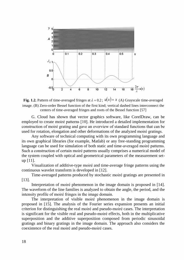
18
Fig. 1.2. Pattern of time-averaged fringes at 2.0 ; xxu (A) Grayscale time-averaged
image. (B) Zero-order Bessel function of the first kind; vertical dashed lines interconnect the
centers of time-averaged fringes and roots of the Bessel function [57]
G. Cloud has shown that vector graphics software, like CorelDraw, can be
employed to create moiré patterns [10]. He introduced a detailed implementation for
construction of moiré grating and gave an overview of standard functions that can be
used for rotation, elongation and other deformations of the analyzed moiré gratings.
Any software of technical computing with its own programming language and
its own graphical libraries (for example, Matlab) or any free-standing programming
language can be used for simulation of both static and time-averaged moiré patterns.
Such a construction of certain moiré patterns usually comprises a numerical model of
the system coupled with optical and geometrical parameters of the measurement set-
up [11].
Visualization of additive-type moiré and time-average fringe patterns using the
continuous wavelet transform is developed in [12].
Time-averaged patterns produced by stochastic moiré gratings are presented in
[13].
Interpretation of moiré phenomenon in the image domain is proposed in [14].
The waveform of the line families is analyzed to obtain the angle, the period, and the
intensity profile of moiré fringes in the image domain.
The interpretation of visible moiré phenomenon in the image domain is
proposed in [15]. The analysis of the Fourier series expansion presents an initial
criterion for distinguishing the real moiré and pseudo-moiré cases. The interpretation
is significant for the visible real and pseudo-moiré effects, both in the multiplicative
superposition and the additive superposition composed from periodic sinusoidal
gratings and binary gratings in the image domain. The approach also considers the
coexistence of the real moiré and pseudo-moiré cases.

19
Moiré effects can be applied in many different fields, including strain analysis,
optical alignment, metrology etc. The moiré fringe method of experimental strain
analysis is applied primarily to solve problems that cannot be solved easily. Typical
problems include: measurements of micro- and nano-structures, high-temperature
measurements, measurement of large elastic and plastic strains without reinforcing
effects in thin films, low-modulus materials, absolute measurements of strain to
establish properties of materials, long-term-stability measurements or measurements
of relatively big structures (civil engineering) over extended period of time.
The projection moiré method that allows to measure the relief of an object or
out-of-plane displacements is presented in [16]. The application of geometric moiré
in large deformation of 3-D models is discussed in [17].
Recent applications using moiré in the fields of material characterization,
micromechanics, microelectronics devices, residual stress, fracture mechanics,
composite materials, and biomechanics are presented in [18]. A detailed research of
moiré fringe method with reference to its application in strain analysis is described
and reviewed in [19]. High precision contouring with moiré and related methods is
reviewed in [20].
1.1.2. Classical visual cryptography and advanced modifications
Visual cryptography is a cryptographic technique which allows visual
information (text, pictures, etc.) to be encrypted in such a way that the decryption can
be performed by the human visual system, without any cryptographic computation –
a simple mechanical operation is enough to perform the decryption. Naor and Shamir
pioneered visual cryptography in 1994 [21]. They determined a visual secret sharing
scheme, where an image was broken up into n shares so that only someone with all
n shares could decrypt the image while anyone with any 1n shares would not
reveal any information about the original image. Each share was printed on a separate
transparency, and the decryption was performed by overlaying the shares. Only if all
n shares were stacked together, the original image would appear. The original
encryption problem can be considered as a 2 out of 2 visual secret sharing problem. It
is recommended to use 4 sub-pixels arranged in 22 arrays where each share has
one of the visual forms in Fig. 1.3.
Fig. 1.3. Sub-pixels arranged in horizontal, vertical and diagonal pairs of 22 arrays for a
pixel sharing [21]
Every pixel of encrypted information is divided into 4 sub-pixels. Due to the
contrast a number of white and black pixels in each array should be the same. A white
20
pixel is splitted into two identical arrays from the list, and a black pixel is shared into
two complementary arrays from the list. Any single pixel of encrypted image in
Share1 is a random choice of 1 out of 6 arrays (Fig. 1.3). The array for each pixel in
Share2 depends on if a black or a white pixel is encoded. If is a white pixel is encoded
– the array should be the same as in Share1 and if there is a black pixel – the array
should be complementary. When two shares are superimposed together, the image is
either medium grey (which represents a white pixel) or completely black (which
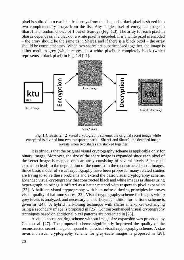
represents a black pixel) in Fig. 1.4 [21].
Fig. 1.4. Basic 22 visual cryptography scheme: the original secret image while
encrypted is divided into two transparent parts – Share1 and Share2; the decoded image
reveals when two shares are stacked together
It is obvious that the original visual cryptography scheme is applicable only for
binary images. Moreover, the size of the share image is expanded since each pixel of
the secret image is mapped onto an array consisting of several pixels. Such pixel
expansion leads to the degradation of the contrast in the reconstructed secret images.
Since basic model of visual cryptography have been proposed, many related studies
are trying to solve these problems and extend the basic visual cryptography scheme.
Extended visual cryptography that constructed black and white images as shares using
hyper-graph colorings is offered as a better method with respect to pixel expansion
[22]. A halftone visual cryptography with blue-noise dithering principles improves
visual quality of halftone shares [23]. Visual cryptography scheme for images with g
grey levels is analyzed, and necessary and sufficient condition for halftone scheme is
given in [24]. A hybrid half-toning technique with shares inter-pixel exchanging
using a secondary image is proposed in [25]. Contrast-enhanced visual cryptography
techniques based on additional pixel patterns are presented in [26].
A visual secret-sharing scheme without image size expansion was proposed by
Chen et al. [27]. The proposed scheme significantly improved the quality of the
reconstructed secret image compared to classical visual cryptography scheme. A size
invariant visual cryptography scheme for gray-scale images is proposed in [28].
21
Decoded gray-scale images of this scheme have higher and clearer contrast with any
unexpected contrast. The newest improvements addressing pixel-expansion and
image quality problem are proposed in [28-31].
Colored visual cryptography scheme that can be easily implemented on the basis
of black and white visual cryptography is presented by Yang and Laih in [32].
Improved visual cryptography schemes for color images are proposed in [33, 34].
Probabilistic visual secret sharing schemes for color and grey-scale images are
proposed in [35].
A visual secret sharing scheme that encodes a set of two or more secrets into
two circle shares such that none of any single share leaks the secrets and the secrets
can be obtained by stacking the first share and the rotated second shares with different
rotation angles is proposed by Shyu et al. [36]. It is the first result that discusses the
sharing ability in visual cryptography up to any general number of multiple secrets in
two circle shares. A multi-secret visual cryptography scheme for 2 out of 2 case when
secret images can be obtained from share images at aliquot stacking angles is proposed
in [37]. A general k out of n shares multi-secret visual cryptography scheme for any k
and n with satisfied security and contrast conditions is proposed in [38]. Visual secret
sharing technique for multiple secrets without pixel expansion is presented in [39].
It can be summarized that the main concept of visual cryptography techniques
based on these features:
Multiple shares scheme: secret image is encrypted into n shares;
Security scheme: original image would appear only if all n shares are
superimposed exactly together, but any combination of superimposed 1n
shares does not reveal any information about the original image;
Encryption scheme: mathematical algorithms are necessary to encrypt the original
image;
Decryption scheme: human visual system can perform the decryption without aid
of computers, only mechanical operation is necessary to superimpose the shares.
The main applications of visual cryptography includes such fields as secure
banking operations and electronic commerce transactions schemes. The authenticity
of the customer signature is based on stacking shares owned by the costumer and the
financial institution [40]. A credit card payment scheme using mobile phones based
on visual cryptography is developed in [41].
Another significant field of visual cryptography applications is biometric
privacy. Visual cryptography technique is adapted onto the area of authentication
using fingerprints. Automatic access control systems deal with falsification and large
database problems. Dividing fingerprint image into two shares, where one share is
kept by the person in the ID card, another share (that is the same for all participants)
is saved in the database helps to compare the stacked image with the provided fresh
fingerprint [42]. Privacy of digital biometric data such as face and fingerprint images
and iris codes can be ensured by dividing data into two separate shares and storing in
two separate database servers [43].
Multimedia security and copyright protection is also significant field of visual
cryptography applications. Attacks resisting video watermarking scheme based on
visual cryptography and scene change detection in discrete wavelet transform domain
22
is proposed in [44]. Resolution variant visual cryptography technique for Street View
of Google Maps is similar to watermarking technique. This secret sharing scheme can
be used to recover specific types of censored information, for example, vehicle
registration numbers [45]. Though the main fields of visual cryptography are
restricted in various forms of information security, visual cryptography can be applied
in young children education. Counting teaching system based on visual cryptography
is described as fun and curiosity stimulating system [46].
1.1.3. Visual cryptography based on moiré techniques
Moiré techniques can be applicable for the cryptography and the protection of
documents. The main applications of the moiré effects for the authentication of
documents and their protection against counterfeiters are presented in [47]. Moiré
based methods can offer solutions to this problem because they can be integrated in
the document without gaining additional production costs.
Low-frequency moiré fringe patterns are employed as a secure numerical code
generator. These moiré patterns are experimentally gained by the superposition of two
sinusoidal gratings with slightly distinct pitches. The numerical code could be used as
standard numerical identification in robotic vision or transmition of security
numerical keys [48, 49].
A halftone image security processing method based on moiré effect is developed
in [50]. Some graphic information are hidden in the pre-copy color images, and then
the images are yielded by means of laser printers and traditional printing proof. When
the specific detecting film is in the right position and angle, the hidden image can be
clearly observed.
One of the first attempts to implement moiré patterns in visual cryptography was
introduced by Desmedt and Le [51]. They provided a scheme where moiré patterns
occur when high-frequency lattices are combined together to produce low-frequency
lattice patterns. As in classical cryptography, the secret image was randomized into
two shares and direct superposition revealed the secret information. There were three
different moiré schemes proposed by Desmedt and Le: lattice rotation, lattice smooth
and dot orientation. Lattice rotation scheme produced visible boundary problem,
while in lattice smooth rotation scheme the artifacts standout and became too much
visible. In dot orientation scheme, diamond shape dots are used to encode a white
pixel by superimposing two squares onto the shares whose dots are oriented at
different angles. Dot patterns that are of the same angle are used to encode the black
pixel. This produces two different moiré patterns for the white and black dots. That
means this scheme uses the moiré patterns to recover the secret embedded image.
Rodriguez presents another technique using computational algorithms based on
optical operations for image encryption and decryption [52]. In this technique, an
image is encrypted by a fringe pattern. This fringe pattern is generated by a
computational algorithm as a cosine function, which added in its argument the
intensity image as a reflectance map. The result of the encryption process is a fringe
pattern deformed according to the image reflectance map. The decryption method is
performed creating a moiré fringe pattern. To carry it out, the encrypted image is
overlapped with a key fringe pattern. This key code is an undeformed fringe pattern,
23
which is generated at the same frequency of the encrypted image. The obtained moiré
pattern is a modulation function, whose envelope corresponds to an approximate
version of the original image. Low pass filter is applied to extract the envelope on the
moiré pattern.
Hidden images constructed on color honeycomb with tiny hexagons moiré
patterns are presented in [53]. The base pattern is a color honeycomb pattern with red,
blue and white hexagons. The screen pattern is a monochrome honeycomb pattern
with a transparent area. If these images are overlapped without shift and rotation, there
can be seen only red hexagons through the transparent part of the screen. However,
by rotating the screen at an overlapping angle, a spotted moiré pattern is generated,
and the spatial frequency periodically changes with the overlapping angle. Because of
the spatial frequency being different on the area of the target image from the
background image, the secret image is clearly visible at the overlapping angles 0 and
30 degrees.
An advantage technique using computational algorithms based on optical
operations on moiré patterns for image encryption and decryption is developed in [54].
In this technique, the image is encrypted by a stochastic geometric moiré pattern
deformed according to the image reflectance map. The stochastic geometrical moiré
pattern and the pixel correlation algorithm are used to encrypt the image. An important
factor of encryption security is that stochastic moiré grating can be deformed in any
direction.
A technique based on oil optical operations and oil moiré patterns for image
hiding is developed in [55]. The encryption is performed by deforming a stochastic
moiré grating in accordance to the grayscale levels of the encrypted image. The quality
of the decrypted image is better-compared to decryption methods based on the
superposition or the regular and deformed moiré gratings.
Contrast enhancement in moiré cryptography framework was developed in [56].
Though moiré cryptography introduced by Desmedt and Van Le produce good quality
shadows without pixel expansion, the secret message is revealed as a moiré pattern,
not as a gray level image, whereas the gray level image simultaneously observable
corresponds to the cover picture. Nevertheless, gray level cover pictures can suffer
from a lack of contrast. The contrast of the cover picture in both the shadow images
and the stacked shadow image has been highly enhanced by randomizing the
orientable halftone cell. In this way, the number of quantization levels is increased as
the square of the width of the halftone cell. As the moiré phenomenon responsible of
the visibility of the message is decoupled from the half-toning of the cover image, it
does not affect the visualization of the message, and it can contribute to the cerebral
separation with the cover picture.
In all reviewed researches, moiré techniques are employed on two or more
shares visual cryptography, and though they produced good quality shadows without
pixel expansion, many of these techniques meet security problems. A detailed analysis
of security and quality issues of visual cryptography schemes is provided in chapter
1.5.
24
1.1.4. Dynamic visual cryptography based on time-averaged fringes produced
by harmonic oscillations
The visual cryptography decoding technique, requiring only one secret image is
considered as an expansion of traditional visual cryptography scheme. The main
principle of basic visual cryptography scheme is to encode the secret image with the
aid of a computer, but decode without computing device is maintained in dynamic
visual cryptography. Dynamic visual cryptography technique is based on the decoding
scheme when the secret image is embedded into a moiré grating and can be interpreted
by a human visual system only when the image is oscillated in a predefined direction
at strictly defined parameters of oscillation [57]. The main features of dynamic visual
cryptography are these:
Secret visual information is embedded into stochastic moiré grating.
Secret information can be revealed only when encoded image is oscillated by a
predetermined trajectory of the motion at strictly defined amplitude of the
oscillation.
Mathematical algorithms are necessary to encrypt the original image, but the
decryption is performed by human visual system.
It is only one share visual cryptography technique.
Image hiding based on optical time-averaging moiré technique is presented in
[57]. Time-averaged digital images are constructed as an integral sum:
1
0
2 2sincos
1lim,
n
kT n
kay
nyxM
; (1.7)
where yxM , is the grayscale level of the surface at point yx, ; is the pitch of
the grating; a is the constant amplitude of oscillation; T is the exposure time; n – the
whole number of k frames. Every frame represents the deflection from the state of
equilibrium and averages of many frames are calculated to form time-averaged digital
images.
The encryption scheme is based on the relationship of the pitch of the grating
, the amplitude of oscillation a and the roots ir of zero-order Bessel function of the
first kind:
ira
2. (1.8)
Let the process of the encoding is presented by an example. The static secret
image consists of two parts: the secret information area and the background. The
encoding algorithm is proposed in detail in [57].
A secret text “KAUNAS” is encoded in a background moiré pattern. The
magnitude of the amplitude is selected to decrypt the image, and the pitch of the
background image 0 can be selected such what ensures that the background moiré
grating will not disappear in the time-averaged image. Next, the pitch for the
encrypted text is selected. The digital image is constructed as a set of vertical columns
25
of pixels, where every vertical column corresponds to a set of grayscale pixels.
Variation of the grayscale level in the area of the background image corresponds to
the pitch 0 . Variation of the grayscale level in the areas occupied by the encrypted
secret text must correspond to one of the pitches calculated from Eq. (1.8).
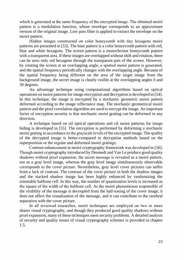
Contrasting boundaries of a background image and encrypted image can reveal
secret information. In order to avoid discontinuities, appropriate phases of the
harmonic variation of the grayscale levels are selected in different zones of the digital
image (Fig. 1.5). The boundaries of the encrypted image and the background image
should match [57].
Fig. 1.5. Matching of phases at boundaries of the background image and the encrypted
image; variations of grayscale levels before the matching (A) and after the matching (B) are
shown [57]
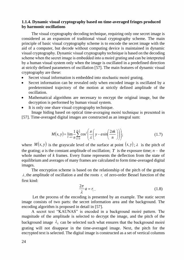
Another security scheme is based on stochastic phase deflection at the top of
adjoining vertical columns of pixels. The procedure is illustrated in Fig. 1.6, where
two adjoining vertical columns of pixels are presented after the initial random phase
at the top of the image (at left in Fig. 1.6) are already assigned. Gray shaded zones in
Fig. 1.6 are plotted different as it is operated with two different columns of pixels. For
secure cryptography scheme it is important to match the phases at boundaries of the
background and the encoded image.
Fig. 1.6. Illustration of the procedure of stochastic deflection of phases for adjoining
columns of pixels (A) and (B) [57]
26
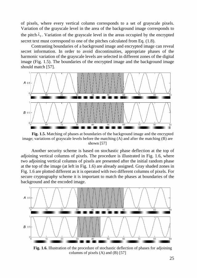
The embedded text “KAUNAS” is seen as a pattern of gray time-averaged
fringes in Fig. 1.7 A (only at appropriate amplitude). Properly pre-selected magnitude
of the amplitude transforms the moiré grating into gray regions in the zone of the
secret text. But the moiré grating in the background is not transformed into a gray area
(Fig. 1.7 A). Alternatively, the background can be transformed into a gray zone at
appropriate amplitude (only one single pitch is used to construct the background moiré
grating). Fig. 1.7 B shows the decoded text which can be clearly distinguished in the
gray background. It is impossible to visualize the image if either the zones
corresponding to the secret text or the background is not transformed into gray time-
averaged fringes (Fig. 1.7 C). The ripples at the top and the bottom of images in Fig.
1.7 are produced by time averaging of boundaries. These ripples are wider, if the
amplitude is higher.
Fig. 1.7. Computational decryption of the encrypted text at three different amplitudes
of harmonic oscillations forms moiré fringes in the encrypted image (A); the background
image (B) and reveals no information (C) [57]
The overall dynamic visual cryptography encoding scheme can be generated by
the following structural polynomial time complexity algorithm:
Input: Secret in digital binary image form.
Output: Cover image.
1. Read the secret digital image.
2. Select the number of pixels comprising the moiré grating for the background
and for the secret.
3. For every column of pixels:
Select a random initial phase of the moiré grating and continue until the
boundary of the secret;
Equalize the phases of the moiré gratings at the boundary between the
boundary and the secret;
Continue the process until the end of the columns.
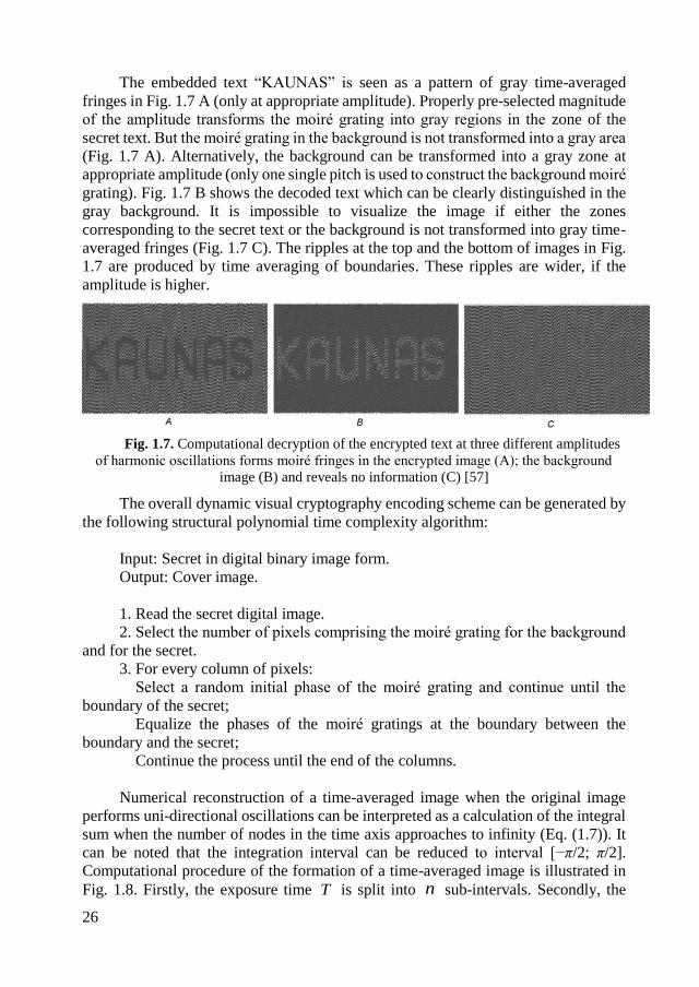
Numerical reconstruction of a time-averaged image when the original image
performs uni-directional oscillations can be interpreted as a calculation of the integral
sum when the number of nodes in the time axis approaches to infinity (Eq. (1.7)). It
can be noted that the integration interval can be reduced to interval [−π/2; π/2].
Computational procedure of the formation of a time-averaged image is illustrated in
Fig. 1.8. Firstly, the exposure time T is split into n sub-intervals. Secondly, the
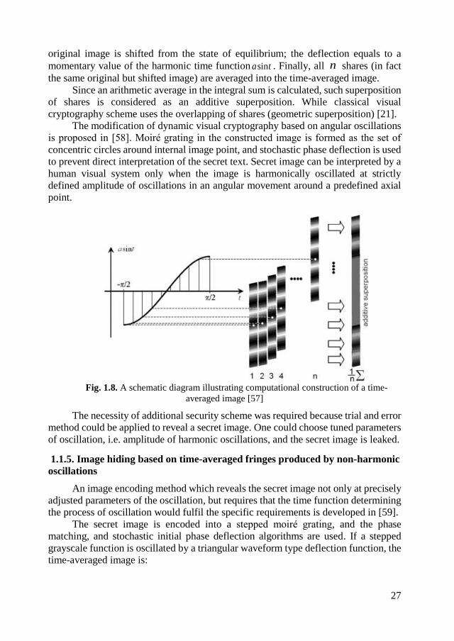
27
original image is shifted from the state of equilibrium; the deflection equals to a
momentary value of the harmonic time function tasin . Finally, all n shares (in fact
the same original but shifted image) are averaged into the time-averaged image.
Since an arithmetic average in the integral sum is calculated, such superposition
of shares is considered as an additive superposition. While classical visual
cryptography scheme uses the overlapping of shares (geometric superposition) [21].
The modification of dynamic visual cryptography based on angular oscillations
is proposed in [58]. Moiré grating in the constructed image is formed as the set of
concentric circles around internal image point, and stochastic phase deflection is used
to prevent direct interpretation of the secret text. Secret image can be interpreted by a
human visual system only when the image is harmonically oscillated at strictly
defined amplitude of oscillations in an angular movement around a predefined axial
point.
Fig. 1.8. A schematic diagram illustrating computational construction of a time-
averaged image [57]
The necessity of additional security scheme was required because trial and error
method could be applied to reveal a secret image. One could choose tuned parameters
of oscillation, i.e. amplitude of harmonic oscillations, and the secret image is leaked.
1.1.5. Image hiding based on time-averaged fringes produced by non-harmonic
oscillations
An image encoding method which reveals the secret image not only at precisely
adjusted parameters of the oscillation, but requires that the time function determining
the process of oscillation would fulfil the specific requirements is developed in [59].
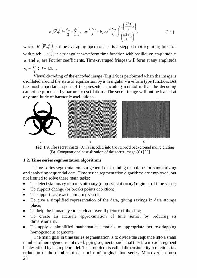
The secret image is encoded into a stepped moiré grating, and the phase
matching, and stochastic initial phase deflection algorithms are used. If a stepped
grayscale function is oscillated by a triangular waveform type deflection function, the
time-averaged image is:
28
sk
sk
xkb
xka
aFH
k
kkss
2
2sin
2cos
2cos
2ˆ;
1
0 ; (1.9)
where ss FH ; is time-averaging operator; F is a stepped moiré grating function
with pitch ; s is a triangular waveform time function with oscillation amplitude s;
ia and ib are Fourier coefficients. Time-averaged fringes will form at any amplitude
2
js j ; ,2,1j .
Visual decoding of the encoded image (Fig 1.9) is performed when the image is
oscillated around the state of equilibrium by a triangular waveform type function. But
the most important aspect of the presented encoding method is that the decoding
cannot be produced by harmonic oscillations. The secret image will not be leaked at
any amplitude of harmonic oscillations.
Fig. 1.9. The secret image (A) is encoded into the stepped background moiré grating
(B). Computational visualization of the secret image (C) [59]
1.2. Time series segmentation algorithms
Time series segmentation is a general data mining technique for summarizing
and analyzing sequential data. Time series segmentation algorithms are employed, but
not limited to solve these main tasks:
To detect stationary or non-stationary (or quasi-stationary) regimes of time series;
To support change (or break) points detection;
To support fast exact similarity search;
To give a simplified representation of the data, giving savings in data storage
place;
To help the human eye to catch an overall picture of the data;
To create an accurate approximation of time series, by reducing its
dimensionality;
To apply a simplified mathematical models to appropriate not overlapping
homogeneous segments.
The main goal in time series segmentation is to divide the sequence into a small
number of homogeneous not overlapping segments, such that the data in each segment
be described by a simple model. This problem is called dimensionality reduction, i.e.
reduction of the number of data point of original time series. Moreover, in most
29
computer science problems, representation of the data is the key to the efficient
solutions. The other goal, as it was mentioned above, is to detect change points of
different, usually non-stationary regimes of time series. These two approaches are
presented in vast number of scientific publications.
Definition of time series segmenting. Let a time series sequence T consisting
of n observations exists: ntttT ,,, 21 , where Rit . A k segmentation S is a
partition of n,,2,1 into k not-overlapping intervals or segments ksssS ,,, 21 ,
such that 11,, ibibi tts , where ib is the beginning of the i-th segment.
One of the simplest method of time series segmentation is sampling, presented
by Astrom in 1969 [60]. There is assumed that an optimal choice of equal spacing step
h in time series of N samples exists.
The method, called piecewise aggregate approximation (PAA), is based on
average value of each segment to represent the corresponding set of data points [61,
62]. An adaptive version of piecewise constant approximation, where the length of
each segment is not fixed, is proposed in [63].
The idea to split time series into most representative segments, and fit a
polynomial model for each segment is presented in [64]. One of the most known time
series representation method is piecewise linear representation (PLR), i.e. an
approximation of a time series of length n with k straight lines. The PLR as time
series segmentation algorithm was adapted in [63]. Following this approach, the PLR
segmentation problems can be described in several approaches:
Time series produce the best representation using only k segments.
Time series produce the best representation such that the maximal error for any
segment does not exceed user specified threshold.
Time series produce the best representation such that the combined error of all
segments does not exceed user specified threshold.
Time series segmentation algorithms can be classified into one of the following
three categories [63]:
Sliding windows: a segment is expanded until it exceeds some error level. The
process is repeated with the next data point that does not belong to the newly
approximated segment. The advantage of this algorithm is its simplicity and the
fact that it is an online algorithm. If a linear approximation is considered, there
are two ways to find the approximated line: linear approximation and linear
regression, taken to be the best fitted in the sense of the least square [64].
Top down: the time series is recursively partitioned until some stopping criteria
is met. This algorithm works by considering every possible partitioning of time
series at splitting it at the best location. Both new segments are then tested to see
if their approximation error is below the some user-specified threshold. If not, the
top down algorithm recursively continues to split the subsequences until all
segments have approximation errors below the threshold. As a segmentation
approach this method is used in [65].
Bottom-up: starting from the most precise possible approximation, segments are
merged until some stop criteria are met. This algorithm is a natural complement
30
to the Top Down algorithm. The algorithm begins by constructing the most precise
possible approximation of the time series, so that n/2 segments are used to
approximate time series of length n. Next, the cost of merging each pair of
adjacent segments is evaluated, and the algorithm starts to iteratively merge the
lowest cost pair until some stopping criteria are met. The bottom-up algorithm has
been used in [66].
Usually, the data do not fit a linear model and the estimation of the local slope
creates over-fitting. Piecewise linear time series segmentation method that adapts time
series model with varying polynomial degree is proposed in [67] as a better
alternative. The adaptive model provides a more precise segmentation than the
piecewise linear model and does not increase the cross-validation error or the running
time. The functionality of the proposed model was tested on synthetic random walks,
electrocardiograms, and historical stock market prices.
Terzi and Tsaparas [68] have also classified the segmentation methods into three
approaches:
Heuristics for solving a segmentation algorithm problem faster than the optimal
dynamic programming algorithm, with promising experimental results but no
theoretical guarantees about the quality of result.
Approximation algorithms with provable error bounds are compared to the
optimal error.
New variations of the basic segmentation problem, imposing some modifications
or constraints on the structure of the representatives of the segments.
Most of the publications published on time series segmentation fall into
heuristics category.
Stationarity is an important factor in the theoretical treatment of time series
procedures. The evolution of complex systems in many cases can be considered being
composed of stationary or quasi-stationary intervals in which time-varying pseudo-
parameters remain more and less unchanged. In general, a proper segmentation of
time series provides a useful portrait of the local properties for investigating and
modelling non-stationary systems. The standard theoretical data analysis approaches
usually rely on the assumption of stationarity and it is important to detect stationary
time series intervals. For example, a well-known ARMA model is a stationary time
series model. Furthermore, the assumption of stationarity is the basis for a general
asymptotic theory: it ensures that the increase of the sample size leads to more
information of the same kind which is the basis for an asymptotic theory to make
sense. On the other hand, many time series from natural and social phenomena exhibit
non-stationarity. Special techniques, such as taking differences or the consideration
of the data on small time intervals have been applied to make an analysis with
stationary techniques possible. If one abandons the assumption of stationarity, the
number of possible models for time series data explodes. For example, one may
consider ARMA models with time varying coefficients.
A non-stationary time-series segmentation method based on the analysis of the
forward prediction error is presented in [69]. Likelihood ratio test based on the
adaptive Schur filter forward prediction error allows the partition of the time-series
31
into homogeneous segments by considering its second-order statistics. The
functionality of the proposed method is performed with simulated signals.
A hybrid evolutionary segmentation method of non-stationary signals based on
fractal dimension and genetic algorithms is presented in [70]. Kalman filter is applied
to reduce the noises and fractal dimension helps to detect the changes in the amplitude
and frequency of the signal. The proposed method is applied to synthetic and real-
world signals.
An adaptive segmentation tool for non-stationary biomedical signals is proposed
in [71]. The implementation is based on the recursive least-squares lattice algorithm
with ability to select system order and the threshold functions. Another adaptive
segmentation algorithm based on wavelet transform and fractal dimension is proposed
in [72].
The problem of modeling a non-stationary time series using piecewise
autoregressive (AR) processes is provided in [73]. The break points of the piecewise
AR segments and the orders of the appropriate AR processes are unknown. The
minimum description length principle is applied to compare if various segmented AR
fits to the data. A combination of the number of segments, the lengths of the segments,
and the orders of the piecewise AR processes is defined as the optimizer of an
objective function, and a genetic algorithm is employed to solve this optimization
problem. An on-line segmentation algorithm based on piecewise autoregressive (AR)
processes is presented in [74]. The algorithm splits up non-stationary time series into
piecewise stationary stochastic signal. Selection of fitting AR model is based on
Akaike's Information Criterion and Yule-Walker equations. A recursive segmentation
procedure for multivariate time series based on Akaike information criterion is
proposed in [75].
Segmentation algorithm for non-stationary time series where each segment is
described by compound Poisson processes with different parameters is proposed in
[76]. The method is applied to financial time series.
A fully non-parametric segmentation algorithm is introduced in [77].
Kalmogorov-Smirnov statistic, which measures the maximal distance between the
cumulative distributions of two samples, is used as an estimate of discrepancy
between segments. This helps to test whether two samples come from the same
distribution without any specification of the distribution.
The problem of estimating multiple structural breaks in a long-memory
fractional autoregressive integrated moving-average (FARIMA) time series is
considered in [78]. The number and the locations of break points, the orders and the
parameters of each regime are assumed to be unknown. A selection criterion based on
the minimum description length principle is proposed and a genetic algorithm is
implemented for its optimization.
Segmentation algorithm which prevents over-segmentation in long-range fractal
correlations is presented in [79]. This algorithm systematically detects only the break
points produced by real non-stationarity but not those created by the correlations of
the signal. The segmentation method is tested to the sequence of the long arm of
human chromosome 21, which has long-range fractal correlations. Similar results
have been achieved when segmenting all human chromosome sequences, showing the

32
existence of previously unknown huge compositional superstructures in the human
genome.
Segmentation algorithm for algebraic progressions is proposed in [80]. It is
shown that it is possible to segment sequence finding a nearest algebraic progression
to an each segment of a given sequence. The proposed segmentation technique based
of the concept of the rank of a sequence that describes exact algebraic relationships
between elements of the sequence. Numerical experiments with an artificially
generated numerical sequence are used to illustrate the functionality of the proposed
algorithm.
Time series streams segmentation is also an important problem in data mining
tasks, because time-series stream is a common data type in data mining. Time series
segmentation algorithms can be classified as batch or online. As it was mentioned,
simple sliding window approach can be considered as online segmentation algorithm,
though more advanced modifications are presented in recent years.
An online algorithm based on sliding window and bottom-up (SWAB)
approaches is presented in [63]. The SWAB scales linearly with the size of dataset
and requires only constant space producing high quality approximations. Empirical
comparisons showed this algorithm to be superior to all others in the literature.
An on-line segmentation method for stream time series data based on turning
points detection is presented in [81]. The turning points are extracted from the
maximum or minimum points of the time series stream.
Another segmentation technique, which can be used in a streaming setting is
proposed in [68]. An alternative constant-factor approximation algorithm DNS have
outperformed other widely-used heuristics.
Online segmentation algorithm based on polynomial least-squares
approximations is presented in [82]. The paper presents SwiftSeg, a technique for
stream time series segmentation and piecewise polynomial representation. Least-
squares approximation of time series in sliding time windows in a basis of orthogonal
polynomials are used to segment time series. The computational effort depends only
on the degree of the approximating polynomial and not on the length of the time
window. SwiftSeg suits for many data streaming applications offering a high accuracy
at very low computational costs.
Parameter-free, real-time, and scalable time-series stream segmenting algorithm
(PRESEE), which greatly improves the efficiency of time-series stream segmenting
is presented in [83]. The PRESEE is based on minimum description length and
minimum message length methods, which segment the data automatically. The
PRESEE test results on empirical data show that the algorithm is efficient for real-
time stream datasets and improves segmenting speed nearly ten times.
An on-line exponential smoothing prediction based segmentation algorithm is
presented in [84]. The algorithm is based on sliding window model and exponential
smoothing method to evaluate the arriving new data value of streaming time series.
Statistical characteristics of prediction error are used to evaluate the fitness to the
segment.
Choosing the number of segments remains a challenging question. An extensive
experimental studies on model selection techniques, Bayesian Information Criterion
33
(BIC) and Cross Validation (CV) are presented in [85]. The segments are identified
with different means or variances and results are given for real DNA sequences with
respect to changes in their codon.
The methodology that deals with the uncertainty in the location of time series
change points is presented in [86]. The evaluation of exact change point distributions
conditional on model parameters via finite Markov chain, and accounting for
parameter uncertainty and estimation via Bayesian modelling and sequential Monte
Carlo.
The applications of time series segmentation algorithms include such fields as
hydrometeorology [87], finance [88, 89, 90], especially, when it is necessary to catch
overall picture in macroeconomics [91, 92, 93], physics [77], biology systems [94,
95]. Segmentation methods are widely used to detect changes in human vital systems
[96, 97], especially, to analyze encephalograms (EEG) [98, 99] and
electrocardiograms (ECG) [100, 101].
Time series segmentation algorithms need some methods to evaluate the quality
of fit for a potential segment. A measure commonly used in conjunction with linear
regression is sum of squares or the residual errors, i.e. by taking all the vertical
differences between the best fit line and the actual data points. Some the most popular
metrics are discussed in chapter 1.3.5 (Metrics to measure forecasting accuracy).
Another commonly used measure of goodness of fit is the distance between the best
fit line and the data point furthest away in the vertical direction.
1.3. Time series forecasting models and algorithms
Time series forecast is a challenging problem in many fields of science and
engineering. Conditionally, time series forecasting could be classified into long-term
time series forecasting techniques and short-term time series forecasting techniques.
In general, the object of time series prediction techniques is to build a model of the
process and then use this model to extrapolate past behavior into the future. One can
classify forecasting methods into smoothing techniques like moving average and
exponential smoothing [102-105], model based methods like ARIMA [106-109],
artificial intelligence methods like ANN (Artificial Neural Network) based models
[110-114], etc. It is agreeable that no single method will outperform all others in all
situations. A short review of forecasting methods and their methodology is reviewed
in this chapter.
Stationary is the main request in model based time series forecasting [106, 115].
Stationary time series are characterized by having a distribution that is independent of
time shifts. This is so called strong stationary. Generally, in practical applications, it
is required that the mean and variance of forecasting processes are constant and the
correlation is only lag dependent (covariance or weak stationary). One of the most
fundamental results of model based time series analysis is Wold decomposition
theorem [116]. It denotes that any stationary process can be written as an infinite sum
of weighted random shocks
1
2211
i
ititttttx ; (1.10)
34
where tx is the process at time t, is the mean of the process; }{ i are uncorrelated
random shocks with zero mean and constant variance, and the coefficients }{ i
satisfies
1
2
i
i .
One of the essential idea of the Box–Jenkins (1970) approach to time series
analysis was their recognition that it was possible to approximate a wide variety of
}{ i weight patterns occurring in practice using models with only a few parameters.
This idea of parsimonious models that led them to introduce the autoregressive
moving average (ARMA) models [106].
The simplest stationary time series process is the white noise [115]. The serially
independent normal white noise (or Gaussian white noise) is the fundamental building
block from which all others models are constructed:
ttx , 2,0~ Nt ; (1.11)
where t are serially uncorrelated, independent and normally distributed random
shocks with zero mean and constant variance 2 .
1.3.1. Model-based time series forecasting methods
One of the well-known and widely applied stationary time series model is first
order autoregression model AR(1) :
ttt xx 110 , 2,0~ Nt ; (1.12)
where 0 , 1 – model coefficients. It is proved that if unit root requirement is fulfilled,
i.e. 11 , the autoregression model is covariance stationary.
Typical example of nonstationary time series model is the random walk model.
ttt xx 1 , 2,0~ Nt . (1.13)
The random walk with drift is a model of stochastic trend. The trend is driven
by stochastic shocks and on average it grows each period by the drift 0
ttt xx 10 , 2,0~ Nt . (1.14)
Generally, the model with shift and deterministic time trend can be written as
ttt txx 110 , 2,0~ Nt ; (1.15)
where is deterministic trend coefficient. This model is used a benchmark of
Dickey-Fuller test to determine whether a unit root is present in an autoregressive
model [117,118]. The finite-order moving average process MA(q) is an
approximation of the Wold (Eq. 1.10) representation, which is an infinite-order
moving average process. The general finite order moving average process of order q
or MA(q):
tt
q
qqtqtttt LLLx θθ1θθθ 12211 ,
2,0~ WNt ; (1.16)
35
where L is the lag operator mtt
m xxL , i – model coefficients,
q
i
i
i LL0
.
The general finite order autoregressive process of order p or AR(p):
tptpttt xxxx 2211 , or
tt
p
t xLLLxL p
2
211
2,0~ WNt ;
(1.17)
where i – model coefficients,
p
i
i
i LL0
.
The ARMA(p,q) process consists of multiple moving average and
autoregressive lags:
tptpttptpttt xxxx θθθ 22112211 ;
2,0~ WNt . (1.18)
ARMA processes can be applied to stationary time series, but, practically, real-
world time series are nonstationary. The type of nonstationary behavior is typically
encountered in many applications is of the type where the level changes, but the
process nevertheless exhibits homogeneity in the variability. In such cases, the (first)
difference 1 ttt xxx , may be stationary. It is refered as being first order
homogenous nonstationary process, or 1I . Another type of nonstationarity
encountered in practice is when both the level and the slope of a time series are
nonstationary, but the variability otherwise exhibits homogeneity. In that case, it is
necessary difference the data twice. The second difference is defined as
21
2 2 tttt xxxx . If the second difference is stationary and homogeneous, it is a
homogeneous nonstationary process of the second order, or 2I . Higher order
differencing is seldom in practice.
Generally, ARIMA(p,d,q) model is expressed like:
tt
dLxLL 1 . (1.19)
The selection of the model sometimes is more art than science. In any modeling
effort, we should always keep in mind that the model is only an approximation of the
true behavior of the system in question. Statistical models contain parameters that
have to be estimated from the data. It is important to employ models with as few
parameters as possible for adequate representation. As opposed to simpler models,
more complicated models with the prodigal use of parameters lead to poor estimates
of the parameters. Models with large number of parameters will tend to overfit the
data, meaning that locally they may provide very good fits; however, globally, that is,
in forecasting, they tend to produce poor forecasts and larger forecast variances [119].
If it is necessary to forecast very short time series, it is helpful to understand the
minimum sample size requirements when fitting statistical models to such data. The
number of data points required for any statistical model depends on at least two things:
the number of model parameters to estimate and the amount of randomness in the data

36
[120]. Box-Jenkins recommendation of sample sizes of at least 50-100 repeat
observations is shown to be reasonable [120].
The general Box-Jenkins model building process is shown in Fig.1.10. The first
step is to visualize data. If there is an obvious nonstationary, the time series should be
differentiated. For stationarity the augmented Dickey–Fuller unit root test is used.
Model identification step is based on two approaches: one can examine plots of
autocorrelation (ACF) and partial autocorrelation (PACF) functions or fit different
possible models and use goodness of fit statistic, for example, Akaike Information
Criterion (AIC) to select better model [121]:
TeTkAICT
t
t
1
22exp ; (1.20)
where k is the number of free model parameters to be estimated; T is the number of
data points of time series; the forecast error is te . In comparison with AIC, Schwarz
Information Criterion (SIC) is also used [122]:
TeTkTSICT
t
t
1
2. (1.21)
The object of model estimation is to minimize the sum of squares of errors.
Widely used metrics to measure forecast errors are defined in chapter 1.3.5.
Fig. 1.10. The Box-Jenkins model building process [106]
37
Model validation is based on examination of residuals. The Ljung–Box test
[123] checks if the data are independently distributed, i.e. the correlations in the
population from which the sample is taken are 0, so that any observed correlations in
the data result from randomness of the sampling process. The statistical significance
of correlation coeficients should be evaluated. Jerque-Berra test [124] is used to test
the normality of residuals. Finally, the estimated model is used to generate forecasts
and usually the confidence limits of the forecasts.
1.3.2. Forecasting based on algebraic methods
For short-term time series forecasting the Hankel matrices can be used. A new
approach to the identification of a numerical sequence and the concept of the Hankel
rank of a sequence is proposed in [125]. The necessary and sufficient conditions of
this concept are proved in [126].
Let a sequence of real or complex numbers is given:
0210 ;:,,, Z kxxxx k . (1.22)
The Hankel matrix (the catelecticant matrix with constant skew diagonals) nH
constructed from the elements of this sequence is defined as follows:
221
21
110
:
nnn
n
n
n
xxx
xxx
xxx
H
; (1.23)
where the index n denotes the order of the square matrix. The determinant of the
Hankel matrix is denoted by nn Hd det ; 1n . The rank of the sequence 0; Zkxk
is such natural number 0; Z kxHrm k that satisfies the following condition [126]:
0kmd ; (1.24)
for all Nk ; but 0nd .
Let us assume that the rank of the sequence is mkxHr k 0; Z ; m . Then
the following equality holds true [126]:
r
k
n
l
lnkkln
k
l
nx
1
1
0
; ,2,1, jjjn ; (1.25)
where characteristic roots Ck ; rk ,,2,1 can be determined from the
characteristic equation
0
1
121
121
10
m
mmm
m
m
xxx
xxx
xxx
; (1.26)
the recurrence indexes of these roots kn ( Nkn ) satisfy the equality
mnnn r 21 ; coefficients Ckl ; rk ,,2,1 ; 1,,1,0 knk can be
38
determined from a system of linear algebraic equations which can be formed from the
systems of equalities in Eq. (1.25).
The set of characteristic roots C kmxxx 1210 ,,, ; Ck ; rk ,,2,1 ;
mnnn r 21 ; 1m is associated to the finite sequence 1210 ,,, mxxx which is
denoted as the base fragment of the algebraic progression [126].
1.3.3. Forecasting based on smoothing methods
Smoothing techniques do not require best-fitting models and do not generally
produce optimal forecasts. A pre-specified model is applied on the data. But these
techniques are useful in situations when model-based forecasting techniques cannot
be used. First, available samples of data are very small where degrees of freedom are
very limited as to render any estimated model of dubious value. Smoothing techniques
require no estimation or minimal estimation. Secondly, smoothing techniques require
little attention, especially, when data are too immense. They are sometimes called
automatic forecasting methods, and they are often useful for forecasting voluminous,
high-frequency data. Finally, smoothing techniques do produce optimal forecasts in
certain conditions, which turn out to be related to the presence of unit roots in the
series being forecast.
The simple moving average process is denoted as
s
xxxx
sx stt
t
s
i
itt
1
1
0
1; (1.27)
where s is the smoothing parameter, the width of averaging process; the larger is s,
the more smoothing is done. The drawback of the moving average method – the first
1s values are lost. The smaller s – the worse effect of moving average, but better
reaction to time series variability and vice versa. If parameter s is relatively large, the
model is equivalent to mean value model. The parameter s is selected so that
forecasting error be smaller and better data representation is completed. If 1s , then
the model is the random walk model (Eq. 1.13), in some references called as naïve
method [127]. If it is necessary to discount the distant past more heavily than the
recent past, the weighted moving average model can be applied:
s
i
itit xx0
; (1.28)
where weights 1 i .
Another simple smoothing technique is simple exponential smoothing method
(SES). Exponential smoothing assigns exponentially decreasing weights over time.
00 xS ,
11 1 ttt SxS ; (1.29)
where 10 is smoothing factor [115]. If smoothing factor is close to 1, past
data have a significant influence on future forecasts. If smoothing factor is close
to 0, the smoothing is relatively slow. The selection of smoothing factor is trial-
and-error process based on smallest forecasting errors. Simple exponential smoothing
39
does not work well when there is a trend in the data [115]. In such situations, Holt-
Winters (1960) double exponential smoothing is used:
111 1 tttt bSxS ,
11 1 tttt bSSb ; (1.30)
where 10 is smoothing factor and 10 is trend smoothing factor.
Smoothing techniques produce point forecasts only, with no attempt to exploit
the stochastic structure of the data to find a best-fitting model, which could be used to
produce interval or density forecasts in addition to point forecasts. They may produce
optimal point forecasts for certain special data generating process, but it is not
assumed that whose special data-generating processes are the truth [115].
1.3.4. Forecasting based on artificial neural networks (ANN)
Artificial neural networks (ANN) are one of the most important types of
nonparametric nonlinear time series models and they are successfully employed in
time series forecasting, including chaotic Mackey-Glass [128,129], financial [130],
stock market [131], electric load [132], hydrologic [133] time series. Neural networks
have been advocated as an alternative to traditional statistical forecasting methods
[129].
One of the most significant advantages of the ANN models over other classes
of nonlinear models is that ANNs can approximate a large class of functions with a
high degree of accuracy [134,135]. Their power comes from the parallel processing
of the information from the data. After learning the data presented to them (a sample),
ANNs can often correctly infer the unseen part of a population even if the sample data
contain noisy information [136]. Opposed to the traditional model-based methods, no
prior assumption of the model form is required in the model building process. Instead,
data-driven self-adaptive network model is largely determined by the characteristics
of the data.
Single hidden layer feed forward network is the most widely used model form
for time series modeling and forecasting [110]. The model is characterized by a
network of three layers of simple processing units connected by acyclic links (Fig.
1.11) [136]. The relationship between the output tx and the inputs pttt xxx ,,, 21
has the following mathematical representation:
t
q
j
p
i
itjijjt exwwfwwx
1 1
,,00 ; (1.31)
where jiw , and jw , pi ,,2,1,0 , qj ,,2,1,0 are model parameters called
connection weights; p is the number of input nodes; and q is the number of hidden
nodes; te – the forecast error.
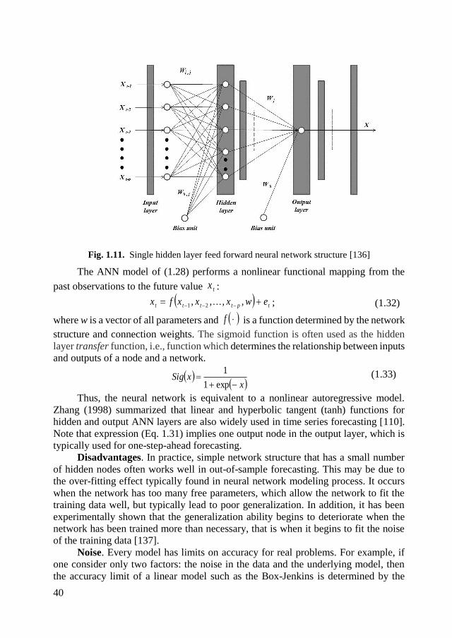
40
Fig. 1.11. Single hidden layer feed forward neural network structure [136]
The ANN model of (1.28) performs a nonlinear functional mapping from the
past observations to the future value tx :
tptttt ewxxxfx ,,,, 21 ; (1.32)
where w is a vector of all parameters and f is a function determined by the network
structure and connection weights. The sigmoid function is often used as the hidden
layer transfer function, i.e., function which determines the relationship between inputs
and outputs of a node and a network.
x
xSig
exp1
1 (1.33)
Thus, the neural network is equivalent to a nonlinear autoregressive model.
Zhang (1998) summarized that linear and hyperbolic tangent (tanh) functions for
hidden and output ANN layers are also widely used in time series forecasting [110].
Note that expression (Eq. 1.31) implies one output node in the output layer, which is
typically used for one-step-ahead forecasting.
Disadvantages. In practice, simple network structure that has a small number
of hidden nodes often works well in out-of-sample forecasting. This may be due to
the over-fitting effect typically found in neural network modeling process. It occurs
when the network has too many free parameters, which allow the network to fit the
training data well, but typically lead to poor generalization. In addition, it has been
experimentally shown that the generalization ability begins to deteriorate when the
network has been trained more than necessary, that is when it begins to fit the noise
of the training data [137].
Noise. Every model has limits on accuracy for real problems. For example, if
one consider only two factors: the noise in the data and the underlying model, then
the accuracy limit of a linear model such as the Box-Jenkins is determined by the

41
noise in the data and the degree to which the underlying functional form is nonlinear.
With more observations, the model accuracy cannot improve if there is a nonlinear
structure in the data. In ANNs, noise alone determines the limit on accuracy due to its
capability of the general function approximation. With a large enough sample, ANNs
can model any complex structure in the data. Hence, ANNs can benefit more from
large samples than linear statistical models can. It can be noted that ANNs do not
necessarily require a larger sample than is required by linear models in order to
perform well. ANN forecasting models perform quite well even with sample sizes
less than 50 while the Box-Jenkins models typically require at least 50 data points in
order to forecast successfully [138, 110].
1.3.5. Combined and hybrid methods for short-term time series forecasting
Improving time series forecasting accuracy is an important, but challenging task
for forecasters. The classical well-known forecasting models and techniques are
reviewed, though the future of time series forecast methods can be based on the
construction and the analysis of hybrid models and combining research [139].
Clements in his editorial suggested more work on combining time series forecast
methods as one possible direction for future research [140]. A combination of models
and methods generally performs better than individual forecast: simple rules for
combining forecasts, such as averages, work as well as ‘optimal weights’ based on the
past performances of the individual forecasts [140]. Both theoretical and empirical
findings have indicated that integration of different models can be an effective way of
improving upon their forecasting performance, especially when the models in the
ensemble are quite different [141].
Hibon and Evgeniou confirmed the hypothesis based on empirical experiments
that when one chooses among methods and their combinations, overall the chosen
individual method may have significantly worse performance than the chosen
combination [142].
Artificial neural networks (ANNs) can be combined with other time series
forecasting methods like autoregressive integrated moving average (ARIMA) models
to take advantage of the unique strength of ARIMA and ANN models in linear and
nonlinear modeling [134, 135]. ARIMA is one of the most widely used linear models
in time series forecasting. ANNs can be an alternative to the traditional linear
methods. A hybrid methodology that combines both ARIMA and ANN models takes
advantage of the unique strength of ARIMA and ANN models in linear and nonlinear
modeling and improves the forecasting accuracy [143]. Another effective hybrid
method as an alternative for artificial neural networks that combines the ARIMA
models and artificial neural networks is proposed in [144]. The ARIMA model is used
to generate the necessary data, and then a neural network is used to determine a model
to capture the underlying data generating process and predict the future, using
preprocessed data. The combination of exponential smoothing model, ARIMA, and
the back propagation neural network model for stock index forecasting is proposed in
[145]. Artificial neural network based models for short-term traffic flow forecasting
using a hybrid exponential smoothing and Levenberg-Marquardt algorithm are
presented in [146]. A hybrid methodology that combines the multilayer perceptron
42
neural networks and Holt exponential smoothing models to forecast stock market time
series is proposed in [147]. Many of the hybrid ARIMA-ANN models firstly apply an
ARIMA model to given time series data, then evaluate the error between the original
and the ARIMA-predicted data as a nonlinear component, and model it using an ANN.
Babu and Reddy firstly use a moving-average filter, and then applies ARIMA and
ANN model [148]. The comparison analysis between the proposed and other hybrid
ARIMA-ANN models showed that the proposed hybrid model has higher prediction
accuracy.
Short-term time series forecasting procedures include different techniques and
models. The use of general exponential smoothing to develop an adaptive short-term
forecasting system based on observed values of integrated hourly demand is explored
in [149]. Short-term load forecasting with exponentially weighted methods is
proposed in [150]. Applications of neural network techniques to short-term load
forecasting are reviewed in [151]. Another short-term load forecasting based on a
semi-parametric additive model is presented in [152]. A similar day-based wavelet
neural network method to forecast tomorrow's load is proposed in [153]. Artificial
neural network (ANN) and Markov chain (MC) are used to develop a new ANN-MC
model for forecasting wind speed in very short-term time scale [154]. Short-term
electricity prices hybrid forecast model that detaches high volatility and daily
seasonality for electricity price based on empirical mode decomposition, seasonal
adjustment and ARIMA is developed in [155]. A novel hybrid approach, combining
adaptive-network-based fuzzy inference system, wavelet transform and particle
swarm optimization for short-term electricity prices forecasting in a competitive
market on the electricity market of mainland Spain is presented in [156]. The radial
basis function ANN with a nonlinear time-varying evolution particle swarm
optimization (PSO) algorithm are used to forecast one-day ahead and five-days ahead
of a practical power system in [157]. PSO algorithms are employed to adjust
supervised training of adaptive ANN in short-term hourly load forecasting in [158].
A new class of moving filtering techniques and of adaptive prediction models that are
specifically designed to deal with runtime and short-term forecast of time series which
originate from monitors of system resources of Internet based servers is developed in
[159].
In spite of numerous amount of forecasting models and techniques, there cannot
be a universal model that will predict everything well for all problems and there will
probably not be a single best forecasting method for all situations [160].
The main objective of the short-term time series methodology proposed in this
dissertation is to enhance the algebraic predictor by employing internal smoothing
procedure that enable reaching a healthy balance between variability of skeleton
algebraic sequences and valuable smoothing properties of predictors based on the
moving averaging methods. The goal is to develop such a predictor which could
produce reliable forecasts for short time series — in situations when the available data
is not enough for such predictors as ARIMA or short term time series nonlinear
forecasting methods such as neural networks or support vector machines.

43
1.3.6. Metrics to measure forecasting accuracy
Accuracy measures are used to evaluate the performance of forecasting
methods. Measurement errors can be classified into: scale-dependent errors,
percentage error, relative errors and scale free errors [161,162]. Regardless of how the
forecast was produced, the forecast error te is simply
ttt oxe ; (1.34)
where tx is a true value of time series element and to is an appropriate observed
value.
One of the simplest scale-dependent measurement method is based on the
average of forecasting errors:
N
i
teN
ME1
1. (1.35)
This metric cannot properly compare different forecasting methods, because it only
shows if averaged process is positive or negative.
A better comparison method is based on the average of absolute forecasting
errors:
N
i
teN
MAE1
1. (1.36)
One of the most widely-used metric is mean squared error:
N
i
teN
MSE1
21. (1.37)
Due to appropriate comparison based on scale units of data, a squared root of mean
square error (RMSE) is used:
N
i
teN
MSERMSE1
21.
(1.38)
Historically, the RMSE and MSE have been popular, largely because of its
theoretical relevance in statistical modelling, however, they are more sensitive to
outliers than MAE [162].
Percentage errors have the advantage of being scale dependent, so they are
frequently used to compare forecast performance between different time series. The
most commonly used metric is mean percentage error (MAPE):
N
i t
t
x
e
NMAPE
1
1.
(1.39)
It is obvious that he MAPE has problems when the series has values close to (or
equal to) zero.
In this dissertation RMSE (Eq. 1.38) and MAE (Eq. 1.36) metrics are used. The
relative performance comparison of different time series methods is also possible,
because the considered time series are transformed into interval [0; 1].
44
1.4. Evolutionary algorithms
1.4.1. Genetic algorithms
Genetic algorithms (GA) and evolutionary algorithms (EA) were introduced by
Holland (1975) and Rechenberg (1973). By imitating basic principles of nature they
created optimization algorithms which have successfully been applied to a wide
variety of problems in engineering, operation research, physics, economics, social
sciences, art, etc. Genetic and evolutionary algorithms and their modifications are
applied as an optimization tool in bioinformatics [163], game theory [164,165], neural
networks [166,167], time series forecasting [168-170], visual cryptography [171,172],
etc.
In artificial intelligence, an evolutionary algorithm (EA) is a subset of
evolutionary computation, a generic population-based meta-heuristic optimization
algorithm. Genetic algorithm is a search heuristic that belong to the larger class of
evolutionary algorithms and imitates the process of natural selection used to generate
solutions to optimization and search problems. These methods generate new points in
the search space by applying operators to current points and statistically moving
toward more optimal places in the search space. Researchers have proposed many
different variants of genetic algorithms in the literature. For illustrating the basic
functionality of GA the traditional standard simple genetic algorithm proposed by
Goldberg (1989) is used [173]. The schematic diagram of genetic algorithms is
presented in Fig. 1.12.
A. Initialization. Initial population of chromosomes is generated for searching
global optimal solution. Usually, the population is generated randomly, allowing the
entire range of the search space. The parameters that are the population size, the
crossover and mutation probabilities, the maximum number of generations and the
termination criterion have to be specified at the initialization process.
B. Evaluation. Every chromosome is evaluated by the fitness function. Fitness
value may be determined by an objective function or by a subjective judgment specific
to the problem. As the generations pass, the members of the population should get
closer to the solution.
C. Selection. Selection is one of the most important operations in the GA
process. The selection operator mainly works at the level of chromosomes. The
goodness of each individual depends on its fitness value determined by an objective
function. Different selection mechanisms work well under different situations. There
are such widely used selection algorithms as roulette wheel selection, rank selection,
tournament selection, steady state selection, Boltzmann selection and elitism
selection.
D. Crossover. The crossover operator is a genetic operator that combines
(mates) two chromosomes (parents) to produce a new chromosome (offspring). The
idea of crossover is based on the assumption that the new chromosome may be better
than both of the parents if it takes the best characteristics from each of them. Crossover
occurs during evolution according to a user definable crossover probability. There is
a number of crossover operators such as: single point crossover, two points’ crossover,
intermediate crossover, arithmetic crossover, heuristic crossover [174].
45
E. Mutation. Mutation is genetic algorithm operator that operates with a
chromosome and randomly modifies the value of a random gene with some mutation
probability. The role of mutation in genetic algorithm is to restore lost or unexplored
tic material into the population to prevent premature convergence of the GA to local
solution.
F. Termination. The process of C-E is repeated until a termination condition
has been reached. The most popular termination criterion is reached predefined
number of generations. But there are some other stopping criteria like elapsed
evolution time, reached fitness threshold and fitness, population or gene convergence
[175].
Initialize
population
Selection
Evaluation
Crossover
Mutation
Termination
criterion
Solution
Yes
No
Update current
population
Fig. 1.12. The schematic diagram of genetic algorithms.
The genetic algorithm may have a tendency to converge towards local optima
rather than the global optimum of the problem for specific optimization problems, and
given the same amount of computation time, simpler optimization algorithms may
find better solutions than genetic algorithms [176].
1.4.2. Particle swarm optimization algorithm
Particle swarm optimization algorithm (PSO) is an evolutionary computation
technique based on the social behavior metaphor, first introduced by Eberhart and
Kennedy in 1995 [177]. Particle swarm optimization is a meta-heuristic procedure and
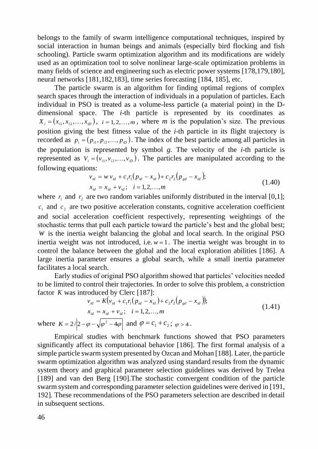
46
belongs to the family of swarm intelligence computational techniques, inspired by
social interaction in human beings and animals (especially bird flocking and fish
schooling). Particle swarm optimization algorithm and its modifications are widely
used as an optimization tool to solve nonlinear large-scale optimization problems in
many fields of science and engineering such as electric power systems [178,179,180],
neural networks [181,182,183], time series forecasting [184, 185], etc.
The particle swarm is an algorithm for finding optimal regions of complex
search spaces through the interaction of individuals in a population of particles. Each
individual in PSO is treated as a volume-less particle (a material point) in the D-
dimensional space. The i-th particle is represented by its coordinates as
iDiii xxxX ,,, 21 , mi ,,2,1 , where m is the population’s size. The previous
position giving the best fitness value of the i-th particle in its flight trajectory is
recorded as iDiii pppp ,,, 21 . The index of the best particle among all particles in
the population is represented by symbol g. The velocity of the i-th particle is
represented as iDiii vvvV ,,, 21 . The particles are manipulated according to the
following equations:
mivxx
xprcxprcvwv
ididid
idgdidididid
,,2,1;
;2211
(1.40)
where 1r and 2r are two random variables uniformly distributed in the interval [0,1];
1c and 2c are two positive acceleration constants, cognitive acceleration coefficient
and social acceleration coefficient respectively, representing weightings of the
stochastic terms that pull each particle toward the particle’s best and the global best; w is the inertia weight balancing the global and local search. In the original PSO
inertia weight was not introduced, i.e. 1w . The inertia weight was brought in to
control the balance between the global and the local exploration abilities [186]. A
large inertia parameter ensures a global search, while a small inertia parameter
facilitates a local search.
Early studies of original PSO algorithm showed that particles’ velocities needed
to be limited to control their trajectories. In order to solve this problem, a constriction
factor K was introduced by Clerc [187]:
mivxx
xprcxprcvKv
ididid
idgdidididid
,,2,1;
;2211
(1.41)
where 42/2 2 K and 21 cc ; 4 .
Empirical studies with benchmark functions showed that PSO parameters
significantly affect its computational behavior [186]. The first formal analysis of a
simple particle swarm system presented by Ozcan and Mohan [188]. Later, the particle
swarm optimization algorithm was analyzed using standard results from the dynamic
system theory and graphical parameter selection guidelines was derived by Trelea
[189] and van den Berg [190].The stochastic convergent condition of the particle
swarm system and corresponding parameter selection guidelines were derived in [191,
192]. These recommendations of the PSO parameters selection are described in detail
in subsequent sections.

47
In comparison with the genetic algorithm (GA), the PSO algorithm is easier to
implement and there are fewer parameters to adjust, the PSO has a more effective
memory capability than the GA and the PSO is more efficient in maintaining the
diversity of the swarm, because in the GA, the worse solutions are discarded and only
the good ones are saved [176]. On the other hand, if one needs to find an optimum of
discrete values, GA algorithm can be more convenient.
1.5. Quality and security aspects of visual cryptography schemes
The analysis of various visual cryptography techniques includes various aspects
of cryptography such as quality and security issues. The necessity to compare classical
and dynamic visual cryptography techniques requires a comprehensive analysis. As it
was mentioned above – visual cryptography is a cryptographic technique which
allows visual information (pictures, text, etc.) to be encrypted in such a way that
decryption becomes a mechanical operation that does not require a computer. The
process of cryptography involves these steps: the plaintext is encrypted, the ciphertext
is sent through the communication channel, and then the decryption is performed to
reveal the plaintext. The same process in ensured in the visual cryptography scheme:
a digital image serves as a plaintext, encryption involves creating shares of the image
which in a sense will be a piece of the image, and then shares are sent to the respective
holders (participants). Decryption involves printing the shares on transparences and
bringing together an appropriate mechanical combination of these shares. The main
principle of visual cryptography is that human visual system is enough to decode the
secret – no additional computations are necessary. One transparency serves as a key,
other transparencies (or a printed pages) are considered as a ciphertext. Separately,
these shares contain random noise. The main advantages of visual cryptography
encryption process – encryption doesn’t require any NP-hard problem dependency
[193]. Decryption is advantageous for its simplicity – a person unknown to
cryptography can decrypt the image. Visual cryptography scheme eliminates complex
computation problem in the decryption process, and the secret images can be restored
by mechanical stacking operation. This property makes visual cryptography
especially useful for the low computation load requirement [194]. Classical visual
cryptography scheme is totally secure – infinite computation power can’t predict the
message.
Dynamic visual cryptography resembles traditional visual cryptography
schemes [57, 59]. The process of dynamic visual cryptography involves the same
steps as used in classical visual cryptography. A digital image serves as a plaintext,
encryption involves embedding of the secret image into the stochastic moiré grating,
and then the encrypted cover image is sent to the receiver. Decryption involves
mechanical oscillation of the cover image. Time averaged image of the oscillating
cover image produces a pattern of time-averaged moiré fringes which are directly
interpreted by the human visual system. Parameters of the oscillation which are used
to decrypt the secret serve as the key, a ciphertext is a single printed cover image.
Decryption algorithm is not required, but a person unknown that the cover image
needs to be oscillated cannot reveal the secret message. The mechanical operation that
performs the decryption to reconstruct the plaintext is implemented with a shaker-
48
table. A finite computation power can predict the message embedded in the cover
image, but dynamic visual cryptography is not prone to cheating (what is not true for
classical visual cryptography). Static cover image resembles a picture of the random
noise; only mechanical oscillation of the cover image does reveal the secret. The main
difference between dynamic visual cryptography and classical visual cryptography is
that dynamic visual cryptography is one share cryptographic technique and
mechanical operation to decrypt the image is based on oscillations – not a simple
geometric superposition of the shares. Dynamic visual cryptography doesn’t require
any NP-hard problem dependency on encryption process [57, 59].
Cryptography aspects of information security such as confidentiality, data
integrity, entity authentication and data origin authentication are essential in visual
cryptography as well [195, 196]. Horng et al. have proved that cheating is possible in
visual cryptography [197]. More secure visual cryptography schemes are provided by
numerous authors and require additional operations to ensure the confidentiality. A
visual cryptography secret sharing scheme allows a secret to be shared only among
authorized participants – any unauthorized participants cannot recover the secret. A
malicious participant can generate the fake shares and the fake image appears when
genuine shares and fake shares are superimposed [197, 198].
One of the most common ways to prevent cheating is extended visual
cryptography schemes that combine traditional visual cryptography with
authentication characteristics. It means that the participants should be able to verify
the integrity of the shares before decoding the secret. Huang and Chang present a non-
expanded visual cryptography scheme with the extra ability of hiding confidential data
to prevent the detection of information by reversing the first share and stacking the
other share [199]. The other way to prevent cheating is based on the construction of
the shares that makes harder for the cheaters to predict the structure of the shares of
the other participants [197]. De Prisco and De Santis’s proposed a cheating prevention
scheme without a complementary image, where the cheaters cannot indicate the actual
value of other participant’s subpixels [200]. Chen etc. proposed a scheme that is
effective against cheating without the more expansion for a pixel, where the number
of the black patterns is used to check whether a share is fake or not [201]. Liu et al.
[202] presented a scheme that avoids usual cheating prevention drawbacks: the
necessity of an online trusted authority, or additional shares for the purpose of
verification, or pixel expansion and contrast reduction of the original visual
cryptography scheme.
While traditional visual cryptography schemes of n shares deal with possibility
to cheat and additional security operations are required to deal with this problem –
dynamic visual cryptography has an advantage as one participant is enough to
implement the decoding process. The secret image is embedded into one share (cover
image) and oscillation of the cover image reveals the secret.
Other possible attacks against visual cryptography include blurring, sharpening,
motion blurring, cropping, filtering and compression. Advanced visual cryptography
schemes implemented on watermarking schemes that are robust to possible attacks
are presented in [203, 204].
49
The analysis of attacks on dynamic visual cryptography schemes is presented in
[205]. It was demonstrated that dynamic visual cryptography is robust to random
noise, Gaussian blur, inappropriate angle of oscillations and vertical shift of secret
share columns, though it is sensitive to the horizontal shift of rows of pixels.
There are various measures and parameters on which performance of visual
cryptography scheme depends, such as the pixel expansion, contrast, accuracy,
computational complexity, meaningfulness or meaningless of the generated shares,
types of secret images (binary or color) and number of secret images (either single or
multiple) encrypted by the scheme [206-210]. Originally Naor and Shamir suggested
two main parameters: pixel expansion and contrast [21]. Pixel expansion refers to the
number of subpixels in the generated shares that represents a pixel of the original input
image. It represents the loss in resolution from the original picture to the shared one.
Contrast is the relative difference in weight between combined shares that come from
a white pixel and a black pixel in the original image. The contrast of reconstructed
image based on original Naor and Shamir scheme is 50%. Jung-San Lee et al. advised
security, pixel expansion, accuracy and computational complexity as performance
measures [211]. Security is satisfied if each share reveals no information of the
original image and the original image cannot be reconstructed if there are fewer than
k shares collected. Accuracy is considered to be the quality of the reconstructed secret
image and evaluated by peak signal-to-noise ratio (PSNR) measure. A high PSNR
implies high accuracy of the secret image sharing scheme. Computational complexity
concerns the total number of operations required both to generate the set of shares and
to reconstruct the original secret image. Both classical and dynamic visual
cryptography algorithms are polynomial time computable – a detailed analysis of non-
expansible visual cryptography algorithm complexity is provided in [212].
Contrast is essential within visual cryptography because it determines the clarity
of the recovered secret by the human visual system. Hofmeister et al. present a linear
solution to the optimal contrast problem. An approach based on coding theory helps
to provide an optimal tradeoff between the contrast and the number of subpixels [213].
Ito’s scheme removes the need for this pixel expansion – the number of subpixels in
a shared pixel is equal to one. The recovered secret can be viewed as the difference of
probabilities with which a black pixel in the reconstructed image is generated from a
white and black pixel in the secret image, but the contrast of recovered image reduces
[214]. Some schemes present methods which do not work with printed transparencies
and these rely on computation in order to recover the secret. In this respect, high
quality secret recovery is possible, however it is preferred if the scheme works with
printed transparencies. A possible option for improving the efficiency of visual
cryptography is to use the XOR operation. Tuyls et al. [215] present a method that
allows traditional stacking of the shares on transparencies, but improves the overall
share quality. The scheme has favorable properties, such as, good resolution and high
contrast, but XOR operation cannot be implemented mechanically without additional
computational efforts.
Dynamic visual cryptography scheme is size invariant visual cryptography
scheme – the size of the share is the same as original image. The quality of the contrast
of dynamic visual cryptography is based on the difference between the pitches of
50
moiré grating embedded at the background and the secret areas. Contrast differences
of the background and the secret image are highest when the pitch of moiré grating of
the secret image is located as far as possible from the pitch of the background [216].
But still the contrast of dynamic visual cryptography remains an important issue,
because the secret image is interpreted as time-averaged moiré fringes – gray zones
of embedded secret (the zones of revealed secret information are completely black in
traditional visual cryptography). This phenomenon yields the necessity to construct
special digital contrast enhancement algorithms, because grayscale levels at
centerlines of fringes depend on the geometrical location of these fringes and
traditional contrast enhancement algorithms fail. Moving average based contrast
enhancement technique that is applied for visualization of time-averaged fringes
produced by time-averaged moiré is presented in [217]. This technique is successfully
implemented in dynamic visual cryptography schemes [57, 59].
A specific aspect of dynamic visual cryptography deals with is the sensitivity to
the oscillation parameters. Dynamic visual cryptography is based not on the static
superposition of moiré images, but on the formation of time-averaged geometric
moiré fringes. The secret is leaked when parameters of oscillations are appropriately
tuned. Malicious participant can decode the secret by trial and error, if only he knows
that he has to shake the share (and also knows the direction of oscillations). The
standard deviation of grayscale level in time-averaged image quantifies the
development of time-averaged moiré fringes [218]. This measure defines the
sensitivity of the decryption of dynamic visual cryptography. The level of the standard
deviation of the time-averaged image showed that the human eye can interpret the
secret image if the standard deviation is not higher than 1% of the width of the interval
of grayscale levels of the cover image [216].
The capacity of a visual cryptography scheme is considered as a maximum
number of secret images embedded into the shares. Naor and Shamir scheme can
embed only one secret image. The maximal size of the hidden information is related
to the size of an image. Advanced visual cryptography schemes can embed a greater
number of secret images into a given image area, which are reconstructed by rotating
one of the stacked shares [219]. Most of visual secret sharing for multiple secrets
schemes decrease the contrast of recovered images while the amount of secret image
encryption increases and additional encryption techniques are necessary to improve
the quality of the recovered image. A novel hybrid encryption algorithm, which splits
the embedding and camouflaging aspects of the encryption process into distinct
phases to adjust the camouflaging density according to the size and thickness of the
ciphertext font, ensures the quality of multiple secrets schemes [220]. Therefore, a
great challenge remains with respect to improving the secret message capacity and the
visual quality of any visual cryptography scheme.
Dynamic visual cryptography is a one-share technique, therefore only one piece
of information can be encrypted in the cover image. The ability to embed more than
one secret into single share that can be revealed with different oscillation parameters
remains the object of the future research.
51
1.6. Concluding remarks
All visual cryptography schemes can be characterized by the same principle that
computational algorithms are necessary to encrypt the image, but the process of the
decryption can be implemented without a computer – a simple mechanical operation
and human visual system are enough for the decryption. Traditional visual
cryptography or moiré cryptography schemes are based on the stacking of two or more
random looking shares, while dynamic visual cryptography is a single share technique
and the decryption is based on the mechanical oscillation operation in a predefined
direction at strictly defined parameters of these oscillations. Though visual
cryptography can be used in a number of important information security applications,
an introduction of oscillations into visual cryptography schemes opens new
possibilities for potential applications of this scheme for optical monitoring of
vibrating structures and testing the human visual system itself. It can be an effective
optical technique for the control vibration generation equipment [216]. But it is well
known that a periodic force applied to nonlinear system can cause a chaotic response
[221]. That creates the necessity to construct dynamic visual cryptography schemes
based on chaotic oscillations. A computational framework for digital implementation
of dynamic visual cryptography is the main aim of the research. That step involves
the development of near-optimal moiré gratings, deformed moiré gratings for the
enhanced security of the secret image. Chaotic dynamic visual cryptography opens
new directions for the applicability of image hiding techniques in a wide pool of
scientific and engineering applications and requires solving a number of important
mathematical and physical problems – which do form the core of this dissertation.
52
2. ADVANCED DYNAMIC VISUAL CRYPTOGRAPHY
The necessity to investigate features of dynamic visual cryptography and to
develop theoretical models and computational framework for digital implementation
is the base of this dissertation. This approach helps to create advanced enhanced
security schemes of dynamic visual cryptography and opens new possibilities to a
wide range of applications.
This chapter of dissertation can be divided into two parts, where quantitative
and qualitative schemes of enhanced dynamic visual cryptography are presented. The
modification with enhanced security based on near-optimal moiré grating, where the
time function determining the process of oscillation is triangular waveform, is
developed in chapter 2.1. A novel dynamic visual cryptography scheme based on the
deformations of the cover image, where the time function determining the process of
oscillation is harmonic, is presented in chapter 2.2.
2.1. Image hiding based on near-optimal moiré gratings
The image hiding method based on time-averaging moiré is proposed in [57].
This dynamic visual cryptography scheme is based not on static superposition of
moiré images, but on time-averaging geometric moiré. This method generates only
one picture which serves as a plaintext; the secret image can be interpreted by the
human visual system only when the original encoded image is harmonically oscillated
in a predefined direction at strictly defined amplitude of oscillation. Parameters of the
oscillation which are used to decrypt the secret serve as the key, a ciphertext is a single
printed cover image. This method resembles a visual cryptography scheme because
one needs a computer to encode a secret, and one can decode the secret without a
computing device. The secret is leaked from encoded picture when parameters of the
oscillation are appropriately tuned. In other words, the secret can be decoded by trial
and error – if only one knows that he has to shake the slide. Therefore, additional
image security measures based on classical visual cryptography scheme are
implemented in [57], particularly breaking up the encoded image into two shares.
Oscillation of any of the shares separately does not reveal the secret. Two shares must
be superimposed and then oscillated harmonically before the secret image can be
interpreted.
The image encoding method which reveals the secret image not only at exactly
tuned parameters of the oscillation, but also requires that the time function
determining the process of oscillation must comply with specific requirements is
developed in [59]. This image hiding method based on time-averaging moiré and non-
harmonic oscillations does not reveal the secret image at any amplitude of harmonic
oscillations. Instead, the secret is leaked only at carefully chosen parameters of this
specific time function (when the density function of the time function is a symmetric
uniform density function). It can be noted that the key to decrypt the image has
additional security parameter – specific time function. Stepped (black and white)
moiré gratings are used in [57] to encode the secret image. The main objective of the
research is to determine if a better moiré grating exists compared to the stepped
53
grating. The criteria for the optimality of the moiré grating is straightforward: no time-
averaged fringes should develop when this grating is oscillated harmonically, and the
secret image should be leaked when the grating is oscillated by the triangular
waveform time function whose density function is a symmetric uniform density
function [222].
2.1.1. Initial definitions and optical background
A one-dimensional moiré grating is considered and some requirements must be
fulfilled for a grayscale function.
Definition 1. Function xF is a grayscale grating function if the following
requirements hold:
Requirement1. The grating is a periodic function; xFxF ; is the pitch
of the grating.
Requirement2. 10 xF ; 0 corresponds to the black color, 1 corresponds to
the white color and all intermediate numerical values of the grating correspond to
an appropriate grayscale level.
Requirement3. xF has only a finite number of discontinuity points in every
finite interval ba; ; ba ( xF is an integrable function).
A harmonic function
xxF
2sin
2
1
2
1~ (2.1)
and a stepped function
1;2
1 ,0
;2
1; ,1
jjxwhen
jjxwhen
xF
(2.2)
are used for the construction of grayscale grating functions for image hiding
applications in [57, 59].
An m-pixels grayscale grating function xF nm, is defined as follows:
j
m
kxj
m
kyxF knm
1 when,, ; (2.3)
where ky , mk ,,2,1 ; Zj are grayscale levels assigned accordingly from a set of
discrete grayscale levels comprising n elements distributed uniformly in the interval
[0;1]. The pixel’s length is m
; m pixels fit into the period of the grayscale grating
function. For example, xF 256,22 represents a grayscale grating function which period
accommodates 22 pixels and the grayscale level of every pixel can be selected from
256 different levels.
The following parameters are used for the characterization of grayscale grating
functions. The supremum and the infimum of the grayscale functions:
54
xFC sup ; (2.4)
xFC inf . (2.5)
The average of the grayscale functions:
0
1dzzF . (2.6)
The norm of the grayscale functions:
0
2
11dzzFxF . (2.7)
Following relationships hold:
10 CxFC ; Rx , (2.8)
2
10 xF . (2.9)
The grayscale function xF can be expanded into the Fourier series:
1
0 2sin
2cos
2 kkk
kxb
kxa
axF
; Rkk ba , ; ,2,1k ; 20 a .
(2.10)
Coefficients of the Fourier expansion and parameters for different grayscale
grating functions read:
1. For the harmonic grayscale grating function xF~
:
10 a ; 0,,, 321 aaa ; 2
11 b ; 0,, 32 bb ; 1C ; 0C ;
2
1 ;
1~xF .
(2.11)
2. For the stepped grayscale grating function xF :
10 a ; 0,,, 321 aaa ;
kb
k
k
111
; ,2,1k ; 1C ; 0C ; 2
1 ;
2
1xF .
(2.12)
3. For the m-pixels grayscale grating function xF nm, :
m
kky
ma
10
2;
m
jjjk
m
kjyy
ka
11
12sin
1
;
m
jjjk
m
kjyy
kb
11
12cos
1
; ,2,1k ;
(2.13)
55
kk
yC max ; k
kyC min ;
m
kky
m 1
1 ;
m
kknm y
mxF
1,
2
11.
Definition 2. The time averaging operator sH is defined as:
;1
lim;0
T
sT
ss dttxFT
FxH (2.14)
where t is time; T is the exposure time; ts is a function describing dynamic
deflection from the state of equilibrium; s is a real parameter; 0s ; Rx .
Two different time functions ts are used. The first one describes the process
of harmonic oscillations:
tsts sin~
; (2.15)
where s is the amplitude; is the angular frequency and is the phase of harmonic
oscillations. Another time function describes the triangular waveform type
oscillations:
;2
32
2
2 when
,2
22
;2
2
2
2 when
,2
22
ˆ
jtj
sjts
jtj
sjts
ts (2.16)
where s is the amplitude; is the frequency and is the phase of triangular waveform
type oscillations. Both functions can be easily implemented experimentally – any
shaker table with appropriate control instrumentation can execute harmonic and
triangular waveform type oscillations.
The averaging operators are [59]:
sk
Jkx
bkx
aa
FxHk
kkss
22sin
2cos
2
~; 0
1
0 (2.17)
and
sk
sk
kxb
kxa
aFxH
k
kkss
2
2sin
2sin
2cos
2ˆ;
1
0; (2.18)
where 0J is zero order Bessel function of the first kind.
Thus, for harmonic time function ts~
, time averaging operator is:
sJxFxH ss
22sin
2
1
2
1~;
~0 . (2.19)
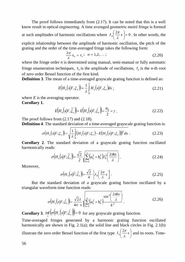
56
The proof follows immediately from (2.17). It can be noted that this is a well
know result in optical engineering. A time averaged geometric moiré fringe is formed
at such amplitudes of harmonic oscillations where 02
0
sJ
. In other words, the
explicit relationship between the amplitude of harmonic oscillation, the pitch of the
grating and the order of the time-averaged fringe takes the following form:
nn rs
2 ; ,2,1n ; (2.20)
where the fringe order n is determined using manual, semi-manual or fully automatic
fringe enumeration techniques, ns is the amplitude of oscillations, nr is the n-th root
of zero order Bessel function of the first kind.
Definition 3. The mean of a time-averaged grayscale grating function is defined as:
0
,1
, dxFxHFxHE ssss ; (2.21)
where E is the averaging operator.
Corollary 1.
2
ˆ,~
, 0aFxHEFxHE ssss . (2.22)
The proof follows from (2.17) and (2.18).
Definition 4. The standard deviation of a time-averaged grayscale grating function is:
0
2;;
1; dxFxHEFxHFxH ssssss . (2.23)
Corollary 2. The standard deviation of a grayscale grating function oscillated
harmonically reads:
1
20
22 2
2
2~;
kkkss
ksJbaFxH
. (2.24)
Moreover,
sJFxH ss
2
4
2~;
~0
. (2.25)
But the standard deviation of a grayscale grating function oscillated by a
triangular waveform time function reads:
1
2
2
22
2sin
4
2ˆ;k
kkssk
ks
bas
FxH
.
(2.26)
Corollary 3. 0ˆ;inf sss
FxH for any grayscale grating function.
Time-averaged fringes generated by a harmonic grating function oscillated
harmonically are shown in Fig. 2.1(a); the solid line and black circles in Fig. 2.1(b)
illustrate the zero order Bessel function of the first type
sJ
20 and its roots. Time-
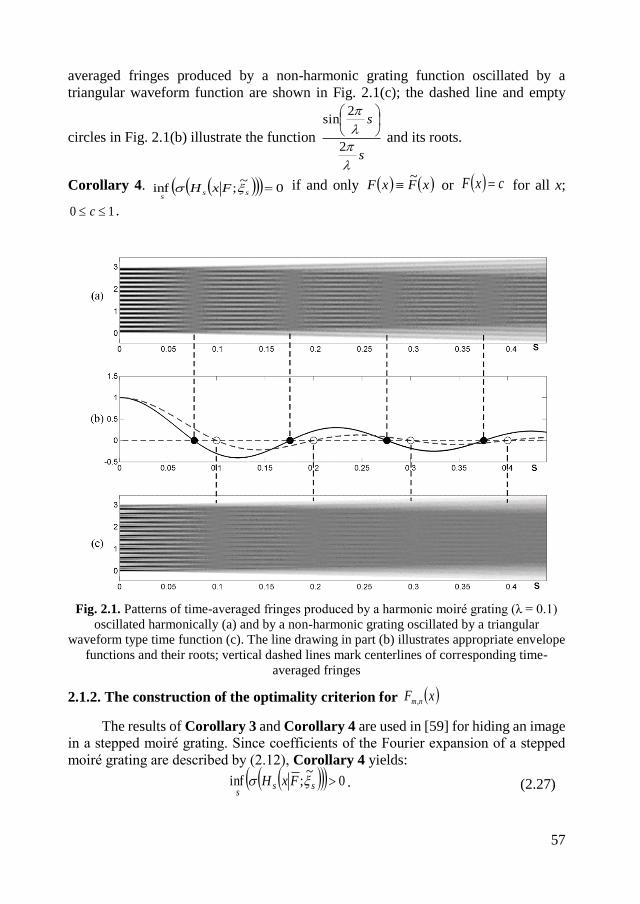
57
averaged fringes produced by a non-harmonic grating function oscillated by a
triangular waveform function are shown in Fig. 2.1(c); the dashed line and empty
circles in Fig. 2.1(b) illustrate the function
s
s
2
2sin
and its roots.
Corollary 4. 0~
;inf sss
FxH if and only xFxF~
or cxF for all x;
10 c .
Fig. 2.1. Patterns of time-averaged fringes produced by a harmonic moiré grating (λ = 0.1)
oscillated harmonically (a) and by a non-harmonic grating oscillated by a triangular
waveform type time function (c). The line drawing in part (b) illustrates appropriate envelope
functions and their roots; vertical dashed lines mark centerlines of corresponding time-
averaged fringes
2.1.2. The construction of the optimality criterion for xF nm,
The results of Corollary 3 and Corollary 4 are used in [59] for hiding an image
in a stepped moiré grating. Since coefficients of the Fourier expansion of a stepped
moiré grating are described by (2.12), Corollary 4 yields:
0~
;inf sss
FxH . (2.27)
58
In other words, time-averaged moiré fringes will not develop when a stepped moiré
grating is oscillated harmonically at any amplitude of oscillations and the embedded
secret image cannot be decrypted by harmonic oscillations (Fig. 2.2). Triangular
waveform type oscillations, on the contrary, enable effective visual decryption of the
secret image.
Fig. 2.2. Undeveloped time-averaged fringes produced by the stepped moiré grating (a) and
the near-optimal moiré grating (b); the pitch of both gratings is λ = 0.1; both gratings are
oscillated harmonically. Full time-average fringes develop when the near-optimal moiré
grating is oscillated by a triangular waveform time function (c)
Therefore the magnitude sss
FxH ~
;inf can be considered as a measure of
the quality of the encryption. The higher is this number, the harder is to interpret the
embedded image when it is oscillated harmonically. The aim of the research is to find
out if the stepped moiré grating xF is an optimal grating (in the sense described
above) or it is possible to find another grayscale grating function for which the lowest
value of the standard deviation of the time-averaged image produced by harmonic
oscillations is higher compared to the stepped moiré grating.
As mentioned previously, a grayscale grating function for which the lowest
value of the standard deviation of the time-averaged image produced by harmonic
oscillations is maximal is sought in this chapter. Unfortunately, this is a very complex
problem of variational optimization. But digital representations of grayscale grating
functions is considered only with m-pixels grayscale grating functions. That simplifies
the optimization problem considerably.
Also, it can be noted that it is not likely that very large amplitudes ( s ) would
be used for the decryption of the embedded image [57, 59]. Thus further simplification
59
of the optimization problem is possible – the minimal value of the standard deviation
will be sought in the interval of amplitudes 1S surrounding the amplitude
2
1r at which
ss FxH ~
;~
reaches its first minimum:
42;
42: 121121
1
rrrrrrS . (2.28)
The variation of standard deviations of xF~
and xF in the interval 1S is
illustrated in Fig. 2.3.
Definition 5. The optimality criterion F for a grayscale grating function F is
defined as follows:
ssSs
FxHF ~
;min1
. (2.29)
It is clear that 0~F . On the other hand, 0467.0F (at 2744.0min s ; Fig.
2.3) is the lower bound of the optimization procedure.
2.1.3. Perfect grayscale grating functions
The optimization problem FnmF
,
max
could be commenced, but first the
definition of a perfect grayscale grating function should be introduced.
Definition 6. xF is a perfect grayscale grating function if four additional
requirements hold true besides the requirements raised in the Definition1:
Requirement 4. The grating spans through the whole grayscale interval: 1C ;
0C .
Requirement 5. The average grayscale level in a pitch of the grating equals to
exactly the middle grayscale level between the white and the black colors: .5.0
Requirement 6. The norm of the grayscale grating function must be at least equal
to the half of the norm of the harmonic grayscale grating:
1~
2
1 xFxF .
Requirement 7. The pitch of the grating must be easily identifiable. The main
peak of the discrete Fourier amplitude spectrum at
2 must be at least two times
higher compared to all other peaks: 222
1
2
1 2 jj baba for all ,3,2j .

60
Fig. 2.3. The variation of standard deviations of the harmonic grayscale grating function (the
dashed line) and the stepped grayscale grating function (the thin solid line) oscillated
harmonically; the thick solid line on the s-axis denotes the interval S1; the empty circle
denotes the amplitude smin where the standard deviation ss FxH ~
;min
of the time-averaged
image reaches its minimum in S1
The necessity of the introduction of perfect grayscale grating functions is
reasoned by the peculiarities of the decryption procedure and the formation of time
averaged moiré fringes (Fig. 2.4). The Requirement 4 forces to use the whole range
of discrete grayscale levels. The Requirement 5 demands that the grayscale level in
the center of a time-averaged fringe is equal to 0.5. The Requirement 6 does not
allow grayscale functions which slightly vary around 0.5 and have only few black and
white pixels in a pitch of the grating. The Requirement 7 demands that the pitch of a
grating must be clearly visible by a naked eye. Otherwise, parasitic time averaged
moiré fringes may form at different amplitudes if, for example, the second peak of the
discrete Fourier amplitude spectrum at
4 is comparable to the main peak at
2.
Corollary 5. xF~
and xF are perfect grayscale functions.
Proof. The proof for xF~
is trivial. The proof for xF is also straightforward:
1
2
1xF , thus the Requirement 6 holds. Coefficients of the Fourier expansion
of xF read: 0,,, 210 aaa ;
12
212
kb k ; 02 kb ; ,2,1k . So,
21 b ; but
kbk
2 ; ,3,2k . Thus, the Requirement 7 holds also. End of proof.
It is clear that xF nm, is not necessarily a perfect grayscale grating function.

61
Fig. 2.4. Illustrations of not perfect grayscale grating functions: (a) – the Requirement 4 does
not hold; the whole range of grayscale levels is not used; (b) – the Requirement 5 does not
hold; the average grayscale level in a pitch does not equal to 0.5; (c) – the Requirement 6
does not hold; the norm of the grayscale grating function is too small; (d) – the Requirement
7 does not hold; the secondary harmonic is too high
Stepped grayscale grating functions comprising 22 pixels in the pitch of the
grating are used to encode digital images in [59]. Here also 22 pixels are used in the
pitch of the grating; 22m . Next, if one chooses 256 different discrete grayscale
levels that would increase the complexity of the solving problem even for evolutionary
algorithms. Instead, as a compromise, 32 different discrete grayscale levels are used
in order to reduce the complexity of the problem and still can be used for practical
implementations. All possible discrete grayscale levels of ky can be enumerated as
31
j ; 31,,2,1,0 j .
Now, finding an optimal perfect 22-pixels grayscale grating function is a
straightforward task. All possible functions xF 32,22 should be generated and checked
if a currently generated function is perfect. If it is a perfect function, 32,22P should
be computed. The highest value of 32,22P produced after the full sorting algorithm
will correspond to the optimal moiré grating. Unfortunately, this full sorting strategy
is unrealistic due to the limited computational resources even after the above-
mentioned simplifications and reductions. Naturally, the alternative objective is to
seek near-optimal moiré gratings. Evolutionary algorithms are used for that purpose.
2.1.4. The construction of evolutionary algorithms
An evolutionary algorithm is constructed in such way that every chromosome
represents one period of a grayscale function xF 32,22 . The length of each chromosome
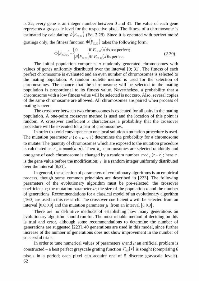
62
is 22; every gene is an integer number between 0 and 31. The value of each gene
represents a grayscale level for the respective pixel. The fitness of a chromosome is
estimated by calculating 32,22F (Eq. 2.29). Since it is operated with perfect moiré
gratings only, the fitness function 32,22F takes the following form:
perfect. is if
perfect;not is if 0
32,2232,22
32,22
32,22xFF
xFF
(2.30)
The initial population comprises n randomly generated chromosomes with
values of genes uniformly distributed over the interval [0; 31]. The fitness of each
perfect chromosome is evaluated and an even number of chromosomes is selected to
the mating population. A random roulette method is used for the selection of
chromosomes. The chance that the chromosome will be selected to the mating
population is proportional to its fitness value. Nevertheless, a probability that a
chromosome with a low fitness value will be selected is not zero. Also, several copies
of the same chromosome are allowed. All chromosomes are paired when process of
mating is over.
The crossover between two chromosomes is executed for all pairs in the mating
population. A one-point crossover method is used and the location of this point is
random. A crossover coefficient κ characterizes a probability that the crossover
procedure will be executed for a pair of chromosomes.
In order to avoid convergence to one local solution a mutation procedure is used.
The mutation parameter μ ( 10 ) determines the probability for a chromosome
to mutate. The quantity of chromosomes which are exposed to the mutation procedure
is calculated as nnm round . Then mn chromosomes are selected randomly and
one gene of each chromosome is changed by a random number r32mod ; here
is the gene value before the modification; r is a random integer uniformly distributed
over the interval 31;0 .
In general, the selection of parameters of evolutionary algorithms is an empirical
process, though some common principles are described in [223]. The following
parameters of the evolutionary algorithm must be pre-selected: the crossover
coefficient ; the mutation parameter ; the size of the population n and the number
of generations. Recommendations for a classical model of an evolutionary algorithm
[160] are used in this research. The crossover coefficient will be selected from an
interval 8.0;6.0 and the mutation parameter from an interval 3.0;0 .
There are no definitive methods of establishing how many generations an
evolutionary algorithm should run for. The most reliable method of deciding on this
is trial and error, although some recommendations to determine the number of
generations are suggested [223]. 40 generations are used in this model, since further
increase of the number of generations does not show improvement in the number of
successful trials.
In order to tune numerical values of parameters and an artificial problem is
constructed – a best perfect grayscale grating function xF 5,6 is sought (comprising 6
pixels in a period; each pixel can acquire one of 5 discrete grayscale levels).
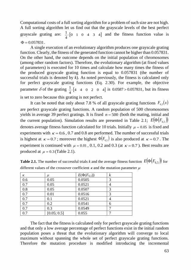
63
Computational costs of a full sorting algorithm for a problem of such size are not high.
A full sorting algorithm let us find out that the grayscale levels of the best perfect
grayscale grating are: 4340104
1 and the fitness function value is
057831.0 .
A single execution of an evolutionary algorithm produces one grayscale grating
function. Clearly, the fitness of the generated function cannot be higher than 0.057831.
On the other hand, the outcome depends on the initial population of chromosomes
(among other random factors). Therefore, the evolutionary algorithm (at fixed values
of parameters) is executed for 10 times and calculate how many times the fitness of
the produced grayscale grating function is equal to 0.057831 (the number of
successful trials is denoted by k). As noted previously, the fitness is calculated only
for perfect grayscale grating functions (Eq. 2.30). For example, the objective
parameter of the grating 4020444
1 is 057831.00587.0 , but its fitness
is set to zero because this grating is not perfect.
It can be noted that only about 7.8 % of all grayscale grating functions xF 5,6
are perfect grayscale grating functions. A random population of 500 chromosomes
yields in average 39 perfect gratings. It is fixed 500n (both the mating, initial and
the current population). Simulation results are presented in Table 2.1; 5,6FE
denotes average fitness function calculated for 10 trials. Initially 05.0 is fixed and
experiments with 6.0 , 0.7 and 0.8 are performed. The number of successful trials
is highest at 7.0 ; moreover the highest 5,6F is also produced at 7.0 . The
experiment is continued with 01.0 , 0.1, 0.2 and 0.3 (at 7.0 ). Best results are
produced at 3.0 (Table 2.1).
Table 2.1. The number of successful trials k and the average fitness function 5,6FE for
different values of the crossover coefficient and the mutation parameter
κ μ E(Φ(F6,5)) k
0.6 0.05 0.0505 3
0.7 0.05 0.0521 4
0.8 0.05 0.0507 3
0.7 0.01 0.0516 3
0.7 0.1 0.0521 4
0.7 0.2 0.0541 6
0.7 0.3 0.0549 7
0.7 [0.05; 0.5] 0.055 7
The fact that the fitness is calculated only for perfect grayscale grating functions
and that only a low average percentage of perfect functions exist in the initial random
population poses a threat that the evolutionary algorithm will converge to local
maximum without spanning the whole set of perfect grayscale grating functions.
Therefore the mutation procedure is modified introducing the incremental
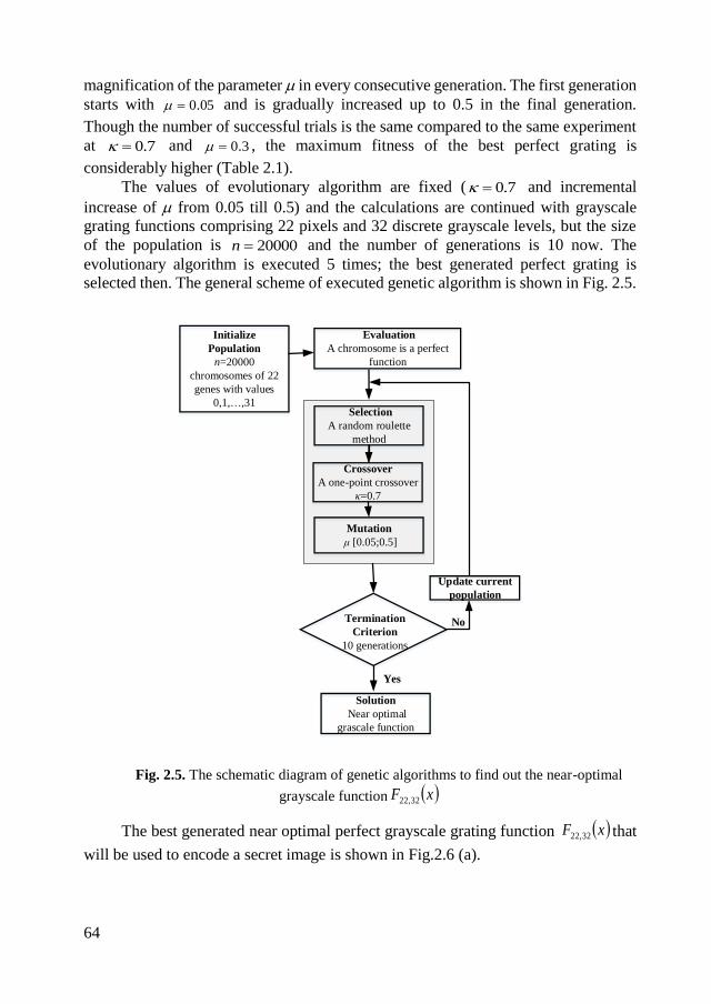
64
magnification of the parameter in every consecutive generation. The first generation
starts with 05.0 and is gradually increased up to 0.5 in the final generation.
Though the number of successful trials is the same compared to the same experiment
at 7.0 and 3.0 , the maximum fitness of the best perfect grating is
considerably higher (Table 2.1).
The values of evolutionary algorithm are fixed ( 7.0 and incremental
increase of from 0.05 till 0.5) and the calculations are continued with grayscale
grating functions comprising 22 pixels and 32 discrete grayscale levels, but the size
of the population is 20000n and the number of generations is 10 now. The
evolutionary algorithm is executed 5 times; the best generated perfect grating is
selected then. The general scheme of executed genetic algorithm is shown in Fig. 2.5.
Initialize
Population
n=20000
chromosomes of 22
genes with values
0,1, ,31 Selection
A random roulette
method
Crossover
A one-point crossover
κ=0.7
Mutation
μ [0.05;0.5]
Termination
Criterion
10 generations
Yes
No
Evaluation
A chromosome is a perfect
function
Solution
Near optimal
grascale function
Update current
population
Fig. 2.5. The schematic diagram of genetic algorithms to find out the near-optimal
grayscale function xF 32,22
The best generated near optimal perfect grayscale grating function xF 32,22 that
will be used to encode a secret image is shown in Fig.2.6 (a).
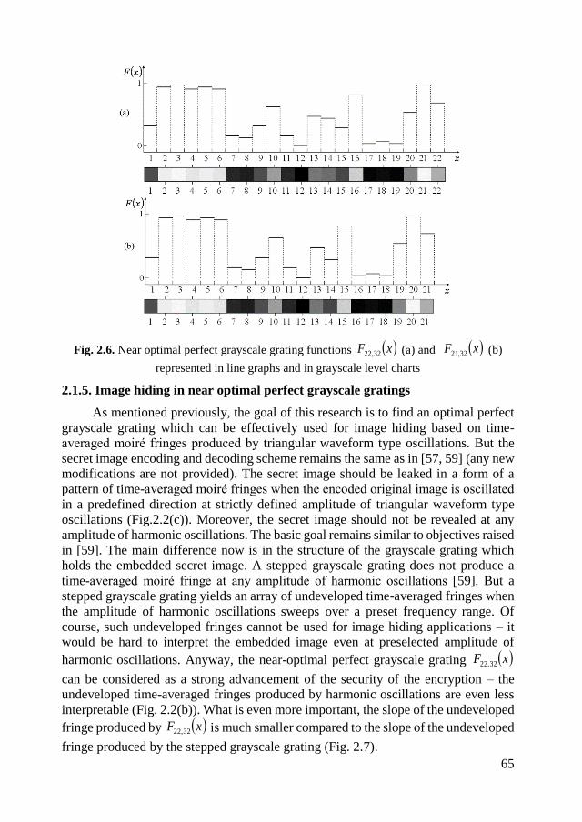
65
Fig. 2.6. Near optimal perfect grayscale grating functions xF 32,22 (a) and xF 32,21 (b)
represented in line graphs and in grayscale level charts
2.1.5. Image hiding in near optimal perfect grayscale gratings
As mentioned previously, the goal of this research is to find an optimal perfect
grayscale grating which can be effectively used for image hiding based on time-
averaged moiré fringes produced by triangular waveform type oscillations. But the
secret image encoding and decoding scheme remains the same as in [57, 59] (any new
modifications are not provided). The secret image should be leaked in a form of a
pattern of time-averaged moiré fringes when the encoded original image is oscillated
in a predefined direction at strictly defined amplitude of triangular waveform type
oscillations (Fig.2.2(c)). Moreover, the secret image should not be revealed at any
amplitude of harmonic oscillations. The basic goal remains similar to objectives raised
in [59]. The main difference now is in the structure of the grayscale grating which
holds the embedded secret image. A stepped grayscale grating does not produce a
time-averaged moiré fringe at any amplitude of harmonic oscillations [59]. But a
stepped grayscale grating yields an array of undeveloped time-averaged fringes when
the amplitude of harmonic oscillations sweeps over a preset frequency range. Of
course, such undeveloped fringes cannot be used for image hiding applications – it
would be hard to interpret the embedded image even at preselected amplitude of
harmonic oscillations. Anyway, the near-optimal perfect grayscale grating xF 32,22
can be considered as a strong advancement of the security of the encryption – the
undeveloped time-averaged fringes produced by harmonic oscillations are even less
interpretable (Fig. 2.2(b)). What is even more important, the slope of the undeveloped
fringe produced by xF 32,22 is much smaller compared to the slope of the undeveloped
fringe produced by the stepped grayscale grating (Fig. 2.7).
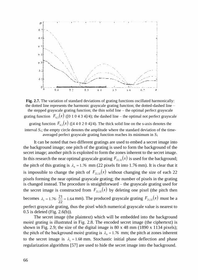
66
Fig. 2.7. The variation of standard deviations of grating functions oscillated harmonically:
the dotted line represents the harmonic grayscale grating function; the dotted-dashed line –
the stepped grayscale grating function; the thin solid line – the optimal perfect grayscale
grating function xF 5,6 ([0 1 0 4 3 4]/4); the dashed line – the optimal not perfect grayscale
grating function xF 5,6 ([4 4 0 2 0 4]/4). The thick solid line on the s-axis denotes the
interval S1; the empty circle denotes the amplitude where the standard deviation of the time-
averaged perfect grayscale grating function reaches its minimum in S1
It can be noted that two different gratings are used to embed a secret image into
the background image; one pitch of the grating is used to form the background of the
secret image; another pitch is exploited to form the zones inherent to the secret image.
In this research the near optimal grayscale grating xF 32,22 is used for the background;
the pitch of this grating is 76.10 mm (22 pixels fit into 1.76 mm). It is clear that it
is impossible to change the pitch of xF 32,22 without changing the size of each 22
pixels forming the near optimal grayscale grating; the number of pixels in the grating
is changed instead. The procedure is straightforward – the grayscale grating used for
the secret image is constructed from xF 32,22 by deleting one pixel (the pitch then
becomes 64.122
2176.11 mm). The produced grayscale grating xF 32,21 must be a
perfect grayscale grating, thus the pixel which numerical grayscale value is nearest to
0.5 is deleted (Fig. 2.6(b)).
The secret image (the plaintext) which will be embedded into the background
moiré grating is illustrated in Fig. 2.8. The encoded secret image (the ciphertext) is
shown in Fig. 2.9; the size of the digital image is 80 x 48 mm (1890 x 1134 pixels);
the pitch of the background moiré grating is 76.10 mm; the pitch at zones inherent
to the secret image is 68.11 mm. Stochastic initial phase deflection and phase
regularization algorithms [57] are used to hide the secret image into the background.
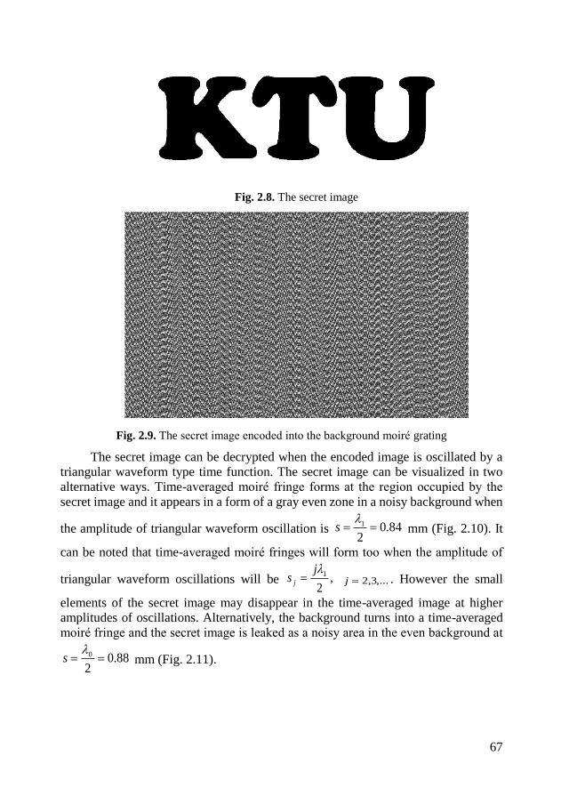
67
Fig. 2.8. The secret image
Fig. 2.9. The secret image encoded into the background moiré grating
The secret image can be decrypted when the encoded image is oscillated by a
triangular waveform type time function. The secret image can be visualized in two
alternative ways. Time-averaged moiré fringe forms at the region occupied by the
secret image and it appears in a form of a gray even zone in a noisy background when
the amplitude of triangular waveform oscillation is 84.02
1
s mm (Fig. 2.10). It
can be noted that time-averaged moiré fringes will form too when the amplitude of
triangular waveform oscillations will be ,2
1js j ,...3,2j . However the small
elements of the secret image may disappear in the time-averaged image at higher
amplitudes of oscillations. Alternatively, the background turns into a time-averaged
moiré fringe and the secret image is leaked as a noisy area in the even background at
88.02
0
s mm (Fig. 2.11).
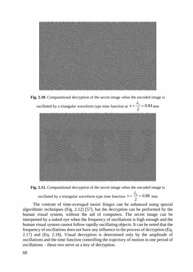
68
Fig. 2.10. Computational decryption of the secret image when the encoded image is
oscillated by a triangular waveform type time function at 84.02
1
s mm
Fig. 2.11. Computational decryption of the secret image when the encoded image is
oscillated by a triangular waveform type time function 88.02
0
s mm
The contrast of time-averaged moiré fringes can be enhanced using special
algorithmic techniques (Fig. 2.12) [57], but the decryption can be performed by the
human visual system, without the aid of computers. The secret image can be
interpreted by a naked eye when the frequency of oscillations is high enough and the
human visual system cannot follow rapidly oscillating objects. It can be noted that the
frequency of oscillations does not have any influence to the process of decryption (Eq.
2.17) and (Eq. 2.18). Visual decryption is determined only by the amplitude of
oscillations and the time function controlling the trajectory of motion in one period of
oscillations – these two serve as a key of decryption.
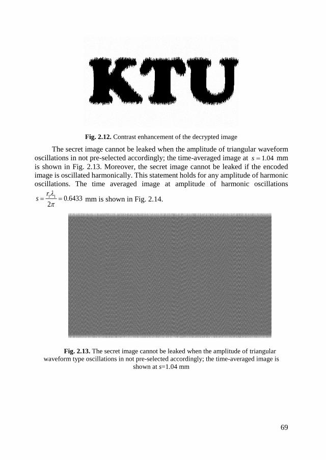
69
Fig. 2.12. Contrast enhancement of the decrypted image
The secret image cannot be leaked when the amplitude of triangular waveform
oscillations in not pre-selected accordingly; the time-averaged image at 04.1s mm
is shown in Fig. 2.13. Moreover, the secret image cannot be leaked if the encoded
image is oscillated harmonically. This statement holds for any amplitude of harmonic
oscillations. The time averaged image at amplitude of harmonic oscillations
6433.02
11
rs mm is shown in Fig. 2.14.
Fig. 2.13. The secret image cannot be leaked when the amplitude of triangular
waveform type oscillations in not pre-selected accordingly; the time-averaged image is
shown at s=1.04 mm
70
Fig. 2.14. The secret image cannot be leaked when oscillations are harmonic; the time-
averaged image is shown at amplitude 6433.0s mm
The PSNR metric between the original image (Fig. 2.8) and the decoded image
(Fig. 2.10) is 9.7312. The contrast of time-averaged moiré fringes can be enhanced
using special algorithmic techniques (Fig. 2.12) [57], but the decryption can be
performed by the human visual system, without the aid of computers. The PSNR
between the original image (Fig. 2.8) and the contrast enhanced image (Fig. 2.12) is
13.1292. This assessment is not very favorable to the proposed technique. It is obvious
that better results could be achieved by other visual cryptography techniques.
Anyway, one must keep in mind that the proposed technique is based on the formation
on time-averaged moiré fringes. Thus a straightforward comparison between classical
and dynamic visual cryptography techniques is irrelevant. The proposed dynamic
visual cryptography scheme works well with larger objects; smaller details are blurred
due to the shorter moiré gratings which are used to encode the secret image. Inevitable
oscillations around the state of the image’s equilibrium cause optical blur at
boundaries of the secret image. What is more important, a whole number of periods
of the moiré grating may not fit into a smaller component of the secret image. This is
a definite drawback of the proposed technique. Anyway, the proposed technique has
a number of advantageous features. This is a single share method; no overlapping of
any shares is required for the formation of the secret image. In this respect a worse
value of the PSNR can be compensated by the added-value of the functionality of the
proposed scheme. The proposed method is not a moiré hash function [224] and the
small change in the initial data (the secret image) does not cause the avalanche effect
in the encrypted image. The proposed technique works well when the size of the secret
geometrical objects is few times greater than the length of one period (pitch) of the
near optimal moiré grating. A small change in one of few pixels in the secret image
would have no effect to the decoded image.
Time needed to encrypt a secret image can be measured using a specific
computational platform. The decryption can be performed completely visually
71
(without a computer) so the assessment of the computational decryption time is
irrelevant (though the decryption time is comparable to the encryption time). The size
of the digital image in Fig. 2.10 is 1890×1134 pixels; it takes 11.8 s to encrypt the
secret image; the computational tool used in the experiments is AMD SempronTM
Processor 3400+, 1.81 GHz, 512 MB RAM.
2.1.6. Concluding remarks on near-optimal moiré gratings
The applicability of image hiding techniques based on time-averaged moiré
fringes is extended. The near-optimal moiré grating provides additional security of
the encoded image, while the decoding procedure is kept completely visual. The main
objective of this research was to optimize the process of encoding, thus one did not
focus on the aspects of the human perception of the vibrating image; computational
experiments have been performed only. A detailed analysis on experimental
implementation of dynamic visual schemes and human perception aspects is provided
in [216].
The shape of the waveform is optimized, where the criterion of optimality is
based on the magnitude of the derivative of the standard deviation at the amplitude
corresponding to the formation of the first moiré fringe. The standard deviation is
computed as the variation of grayscale levels around the mean grayscale level in the
time averaged image while the derivative of the standard deviation in respect to the
amplitude of a piece-wise uniform waveform defines the applicable interval of
amplitudes for visual decryption of the secret image. Experimental implementation
showed that the secret image is interpretable if the standard deviation is not higher
than 0.01 [216].
The developed image hiding technique resembles visual cryptography method,
though the secret image is not split into shares; all information on the secret is kept in
one image. The interplay between moiré gratings, stochastic initial phase scrambling
and phase regularization algorithms are used to encode the secret into the carrier
image. It is important to note that a computer is not necessary to decode the image –
a naked eye can interpret the embedded secret if the encoded image is oscillated in a
predefined direction at predefined amplitude and according to a predefined time
function. Though the contrast is not a strength side of the proposed scheme – it can be
applied as an effective optical technique for the control vibration generation
equipment.
72
2.2. Image hiding in time-averaged deformable moiré gratings
Time averaged geometric moiré can be exploited not only for the optical
analysis of vibrating structures but also for the synthesis of a predefined pattern of
time-averaged fringes. Such type of image hiding technique when the secret image
leaks in a form of a time-averaged moiré fringe in an oscillating non-deformable cover
image was presented in [57]. Stochastic moiré grating is used to embed the secret into
a single cover image – the secret can be visually decoded by a naked eye only when
the amplitude of the harmonic oscillations does correspond to an accurately
preselected value. The fact that a naked eye cannot interpret the secret from a static
cover image makes this image hiding technique similar to visual cryptography –
special computational algorithms are required to encode the image, but the decoding
is completely visual. The difference from visual cryptography is that only a single
cover image is used and that it should be oscillated in order to leak the secret. And
though the cover image is not cryptographically secure such fusion of time averaged
geometric moiré and visual cryptography deserves the title of dynamic visual
cryptography [57]. Different measures have been exploited to increase the security of
dynamic visual cryptography. Near-optimal moiré gratings [222], triangular
waveforms [59] have been used as additional security measures of the scheme (chapter
2.1). It is important to note that visual decoding of all these dynamic visual
cryptography schemes is based on a non-deformable moiré grating – the cover image
is oscillated, but not deformed. A natural question does arise if dynamic visual
cryptography scheme could be implemented on a deformable moiré grating and a new
type of mechanical operation that ensures the decryption of the secret image could be
considered as additional parameter of the dynamic visual cryptography key. The
research based on this assumption is presented in chapter 2.2.
2.2.1. A non-deformable moiré grating with a constant pitch.
Let us consider a one-dimensional harmonic moiré grating:
xxF
2cos
2
1
2
1; (2.31)
where is the pitch of the grating; 0 corresponds to the black color, 1 corresponds to
the white color and all intermediate numerical values of xF correspond to an
appropriate grayscale level. Let us assume that this moiré grating is painted on the
surface of one-dimensional non-deformable body. Also, let us assume that this body
oscillates around the state of equilibrium (without being deformed) and the deflection
from state of equilibrium does not depend on x:
tatutxu sin, ; (2.32)
where is the cyclic frequency, φ is the phase and a is the amplitude of oscillation.
The resultant time-averaged image reads [57]:
aJxdttaxFT
xF
T
T
22cos
2
1
2
1sin
1lim 0
0
;
(2.33)
73
where T is the exposure time; 0J is the zero order Bessel function of the first kind.
The original moiré grating is mapped into a time-averaged fringe ( 2
1xF ) when
0J becomes equal to zero. In other words, the explicit relationship among the pitch of
the moiré grating , the amplitude of harmonic oscillations a and the consecutive
number of the time-averaged moiré fringe k reads:
kk ra
2; ,2,1k ; (2.34)
where kr is the k-th root of 0J ; ka is the discreet value of the amplitude which results
into the k-th time-averaged fringe in the time-averaged image.
2.2.2. A deformable moiré grating with a constant pitch
Now let us consider the same moiré grating (Eq. (2.31)) plotted on the surface
of a one-dimensional deformable body. Let us assume that the left end of this linear
deformable body is motionlessly fixed at 0x and the right end is free at 1xx in
the state of equilibrium. Let us assume that the amplitude of harmonic oscillations is
equal to 1Ax at 1xx . Now the deflection from state of equilibrium does depend on
x:
tAxtxu sin, ; 10 xx . (2.35)
The instantaneous shape of the deformed grating dF reads:
xFtxuxFd , . (2.36)
It would be tempting to express dF is the following explicit form:
txuxFtxFd ,, , (2.37)
but such transition leads to a crude mathematical error [224] – such explicit expression
holds only if txu , does not depend on x. Otherwise (if one wishes to construct an
explicit form of dF ), it is necessary to express x in terms of z from the following
equality:
ztxux , (2.38)
Luckily, it is possible to solve (2.38) when Eq. (2.35) holds. Thus, the explicit
instantaneous expression of dF reads [224]:
x
tAtA
xFtxFd
sin1
2cos
2
1
2
1
sin1, . (2.39)
Now, the time-averaged image reads:
2
00
,2
1,
1lim dttxFdttxF
TxF d
T
dT
d . (2.40)
Unfortunately, the definite integral in Eq. (2.40) cannot be expressed in a form
comprising ordinary functions. Nevertheless, an explicit expression of Eq. (2.40) is
constructed in [224] in a form of infinite function series:

74
0
2
2!2
1
2
1
j
j
jd
A
j
SxF ; (2.41)
where
xS
2cos0 ;
0
12
12
2122
!12
12
k
k
j
k
j xjkk
xS
;
(2.42)
where the factorial structure nm is defined as follows:
1:0 m ; mm :1 ; 11 nmmmm m ; 0Zm ; Nn . (2.43)
Direct interpretation of Eq. (2.41) is impossible due to the interplay of infinite
functional series. Computational interpretation of xFd is presented in [224] and
suggests that the formation of time-averaged fringes induced by an oscillating
deformable moiré grating is somewhat similar to Eq. (2.33) under the assumption that
the amplitude a increases continuously with x. This fact can be illustrated by the
following reasoning. Eq. (2.39) yields:
2sin
22cos
2
1
2
1, AOxtAxtxFd
. (2.44)
Let us assume that A is not large. Note that Eq. (2.39) is defined only at 10 A
(a singularity exists at 1A ). Then, neglecting higher order terms, results into the
following approximation of (2.44):
.sin2
sin2
sin2
1
sin2
cos2
cos2
1
2
1,
xtAx
xtAxtxFd
(2.45)
It is easy to prove that
0sin2
sin
2
0
dtxtA , (2.46)
because the sine function is an odd function. Then,
.22
cos2
1
2
1
sin2
cos1
lim2
cos2
1
2
1
0
0
AxJx
dtxtAT
xxF
T
Td
(2.47)
Therefore, time-averaged moiré fringes induced by an oscillating deformable
grating with a constant pitch do form at such x where:
A
rx k
2 ; ,2,1k , (2.48)
and the envelope function dE modulating the stationary grating can be approximated:
AxJxEd
2
2
1
2
10 . (2.49)
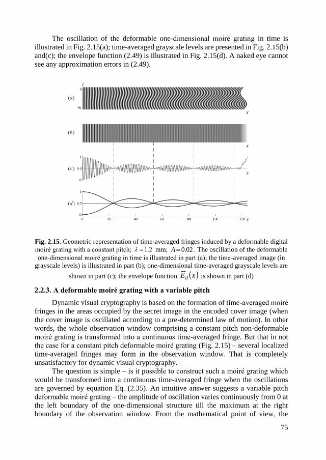
75
The oscillation of the deformable one-dimensional moiré grating in time is
illustrated in Fig. 2.15(a); time-averaged grayscale levels are presented in Fig. 2.15(b)
and(c); the envelope function (2.49) is illustrated in Fig. 2.15(d). A naked eye cannot
see any approximation errors in (2.49).
Fig. 2.15. Geometric representation of time-averaged fringes induced by a deformable digital
moiré grating with a constant pitch; 2.1 mm; 02.0A . The oscillation of the deformable
one-dimensional moiré grating in time is illustrated in part (a); the time-averaged image (in
grayscale levels) is illustrated in part (b); one-dimensional time-averaged grayscale levels are
shown in part (c); the envelope function xEd is shown in part (d)
2.2.3. A deformable moiré grating with a variable pitch
Dynamic visual cryptography is based on the formation of time-averaged moiré
fringes in the areas occupied by the secret image in the encoded cover image (when
the cover image is oscillated according to a pre-determined law of motion). In other
words, the whole observation window comprising a constant pitch non-deformable
moiré grating is transformed into a continuous time-averaged fringe. But that in not
the case for a constant pitch deformable moiré grating (Fig. 2.15) – several localized
time-averaged fringes may form in the observation window. That is completely
unsatisfactory for dynamic visual cryptography.
The question is simple – is it possible to construct such a moiré grating which
would be transformed into a continuous time-averaged fringe when the oscillations
are governed by equation Eq. (2.35). An intuitive answer suggests a variable pitch
deformable moiré grating – the amplitude of oscillation varies continuously from 0 at
the left boundary of the one-dimensional structure till the maximum at the right
boundary of the observation window. From the mathematical point of view, the
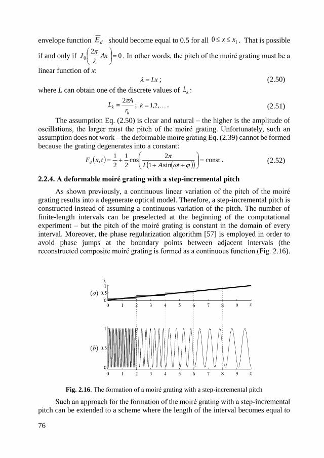
76
envelope function dE should become equal to 0.5 for all 10 xx . That is possible
if and only if 02
0
AxJ
. In other words, the pitch of the moiré grating must be a
linear function of x:
Lx ; (2.50)
where L can obtain one of the discrete values of kL :
kk
r
AL
2 ; ,2,1k . (2.51)
The assumption Eq. (2.50) is clear and natural – the higher is the amplitude of
oscillations, the larger must the pitch of the moiré grating. Unfortunately, such an
assumption does not work – the deformable moiré grating Eq. (2.39) cannot be formed
because the grating degenerates into a constant:
constsin1
2cos
2
1
2
1,
tALtxFd
. (2.52)
2.2.4. A deformable moiré grating with a step-incremental pitch
As shown previously, a continuous linear variation of the pitch of the moiré
grating results into a degenerate optical model. Therefore, a step-incremental pitch is
constructed instead of assuming a continuous variation of the pitch. The number of
finite-length intervals can be preselected at the beginning of the computational
experiment – but the pitch of the moiré grating is constant in the domain of every
interval. Moreover, the phase regularization algorithm [57] is employed in order to
avoid phase jumps at the boundary points between adjacent intervals (the
reconstructed composite moiré grating is formed as a continuous function (Fig. 2.16).
Fig. 2.16. The formation of a moiré grating with a step-incremental pitch
Such an approach for the formation of the moiré grating with a step-incremental
pitch can be extended to a scheme where the length of the interval becomes equal to
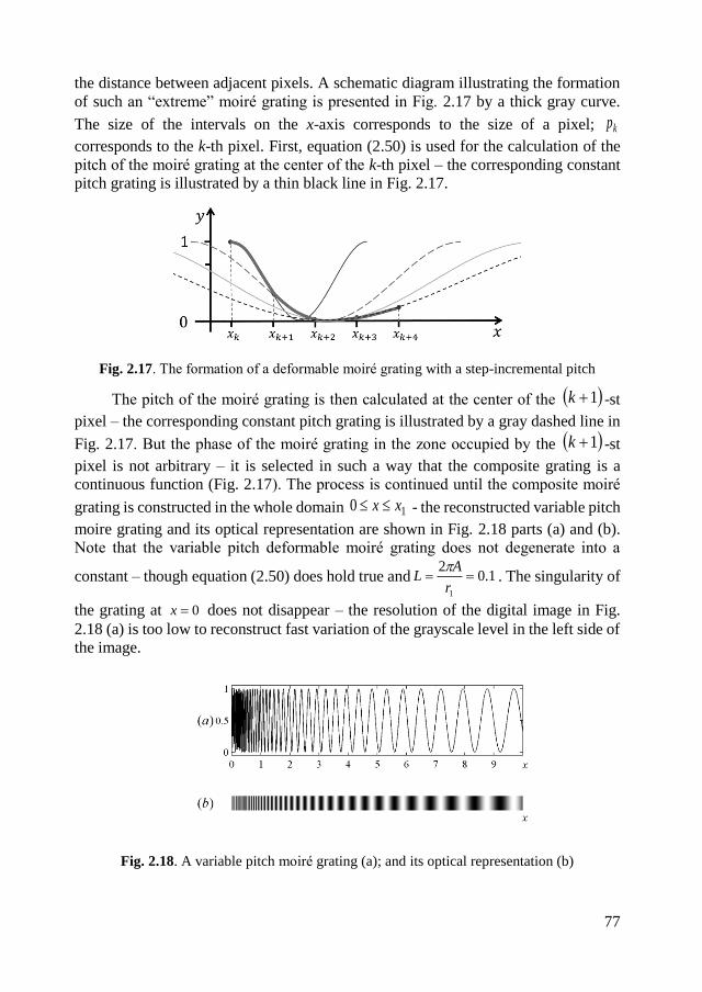
77
the distance between adjacent pixels. A schematic diagram illustrating the formation
of such an “extreme” moiré grating is presented in Fig. 2.17 by a thick gray curve.
The size of the intervals on the x-axis corresponds to the size of a pixel; kp
corresponds to the k-th pixel. First, equation (2.50) is used for the calculation of the
pitch of the moiré grating at the center of the k-th pixel – the corresponding constant
pitch grating is illustrated by a thin black line in Fig. 2.17.
Fig. 2.17. The formation of a deformable moiré grating with a step-incremental pitch
The pitch of the moiré grating is then calculated at the center of the 1k -st
pixel – the corresponding constant pitch grating is illustrated by a gray dashed line in
Fig. 2.17. But the phase of the moiré grating in the zone occupied by the 1k -st
pixel is not arbitrary – it is selected in such a way that the composite grating is a
continuous function (Fig. 2.17). The process is continued until the composite moiré
grating is constructed in the whole domain 10 xx - the reconstructed variable pitch
moire grating and its optical representation are shown in Fig. 2.18 parts (a) and (b).
Note that the variable pitch deformable moiré grating does not degenerate into a
constant – though equation (2.50) does hold true and 1.02
1
r
AL
. The singularity of
the grating at 0x does not disappear – the resolution of the digital image in Fig.
2.18 (a) is too low to reconstruct fast variation of the grayscale level in the left side of
the image.
Fig. 2.18. A variable pitch moiré grating (a); and its optical representation (b)
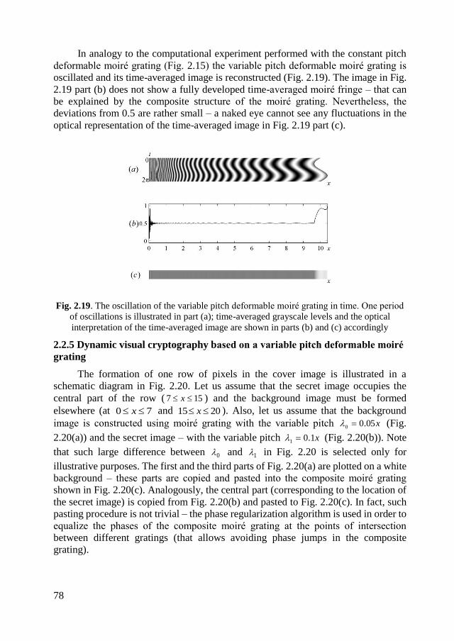
78
In analogy to the computational experiment performed with the constant pitch
deformable moiré grating (Fig. 2.15) the variable pitch deformable moiré grating is
oscillated and its time-averaged image is reconstructed (Fig. 2.19). The image in Fig.
2.19 part (b) does not show a fully developed time-averaged moiré fringe – that can
be explained by the composite structure of the moiré grating. Nevertheless, the
deviations from 0.5 are rather small – a naked eye cannot see any fluctuations in the
optical representation of the time-averaged image in Fig. 2.19 part (c).
Fig. 2.19. The oscillation of the variable pitch deformable moiré grating in time. One period
of oscillations is illustrated in part (a); time-averaged grayscale levels and the optical
interpretation of the time-averaged image are shown in parts (b) and (c) accordingly
2.2.5 Dynamic visual cryptography based on a variable pitch deformable moiré
grating
The formation of one row of pixels in the cover image is illustrated in a
schematic diagram in Fig. 2.20. Let us assume that the secret image occupies the
central part of the row ( 157 x ) and the background image must be formed
elsewhere (at 70 x and 2015 x ). Also, let us assume that the background
image is constructed using moiré grating with the variable pitch x05.00 (Fig.
2.20(a)) and the secret image – with the variable pitch x1.01 (Fig. 2.20(b)). Note
that such large difference between and in Fig. 2.20 is selected only for
illustrative purposes. The first and the third parts of Fig. 2.20(a) are plotted on a white
background – these parts are copied and pasted into the composite moiré grating
shown in Fig. 2.20(c). Analogously, the central part (corresponding to the location of
the secret image) is copied from Fig. 2.20(b) and pasted to Fig. 2.20(c). In fact, such
pasting procedure is not trivial – the phase regularization algorithm is used in order to
equalize the phases of the composite moiré grating at the points of intersection
between different gratings (that allows avoiding phase jumps in the composite
grating).
0 1
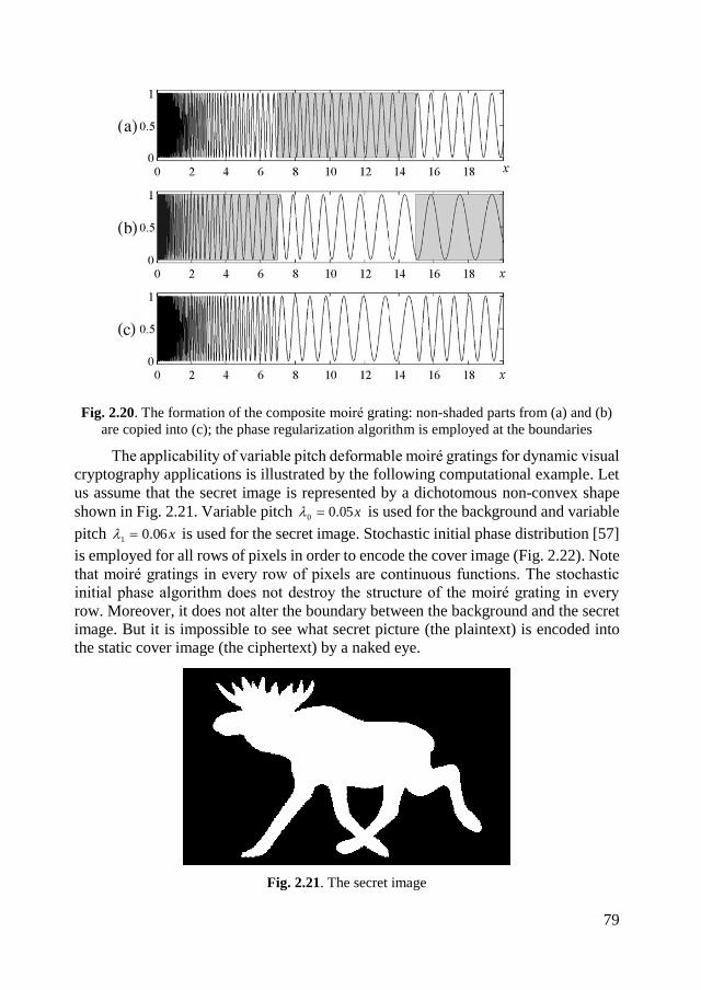
79
Fig. 2.20. The formation of the composite moiré grating: non-shaded parts from (a) and (b)
are copied into (c); the phase regularization algorithm is employed at the boundaries
The applicability of variable pitch deformable moiré gratings for dynamic visual
cryptography applications is illustrated by the following computational example. Let
us assume that the secret image is represented by a dichotomous non-convex shape
shown in Fig. 2.21. Variable pitch x05.00 is used for the background and variable
pitch x06.01 is used for the secret image. Stochastic initial phase distribution [57]
is employed for all rows of pixels in order to encode the cover image (Fig. 2.22). Note
that moiré gratings in every row of pixels are continuous functions. The stochastic
initial phase algorithm does not destroy the structure of the moiré grating in every
row. Moreover, it does not alter the boundary between the background and the secret
image. But it is impossible to see what secret picture (the plaintext) is encoded into
the static cover image (the ciphertext) by a naked eye.
Fig. 2.21. The secret image
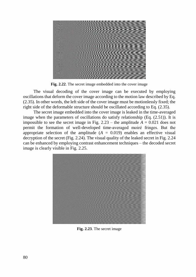
80
Fig. 2.22. The secret image embedded into the cover image
The visual decoding of the cover image can be executed by employing
oscillations that deform the cover image according to the motion law described by Eq.
(2.35). In other words, the left side of the cover image must be motionlessly fixed; the
right side of the deformable structure should be oscillated according to Eq. (2.35).
The secret image embedded into the cover image is leaked in the time-averaged
image when the parameters of oscillations do satisfy relationship (Eq. (2.51)). It is
impossible to see the secret image in Fig. 2.23 – the amplitude A = 0.021 does not
permit the formation of well-developed time-averaged moiré fringes. But the
appropriate selection of the amplitude (A = 0.019) enables an effective visual
decryption of the secret (Fig. 2.24). The visual quality of the leaked secret in Fig. 2.24
can be enhanced by employing contrast enhancement techniques – the decoded secret
image is clearly visible in Fig. 2.25.
Fig. 2.23. The secret image
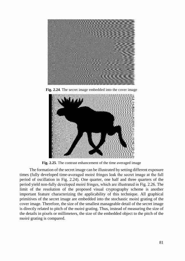
81
Fig. 2.24. The secret image embedded into the cover image
Fig. 2.25. The contrast enhancement of the time averaged image
The formation of the secret image can be illustrated by setting different exposure
times (fully developed time-averaged moiré fringes leak the secret image at the full
period of oscillation in Fig. 2.24). One quarter, one half and three quarters of the
period yield non-fully developed moiré fringes, which are illustrated in Fig. 2.26. The
limit of the resolution of the proposed visual cryptography scheme is another
important feature characterizing the applicability of this technique. All graphical
primitives of the secret image are embedded into the stochastic moiré grating of the
cover image. Therefore, the size of the smallest manageable detail of the secret image
is directly related to pitch of the moiré grating. Thus, instead of measuring the size of
the details in pixels or millimeters, the size of the embedded object to the pitch of the
moiré grating is compared.
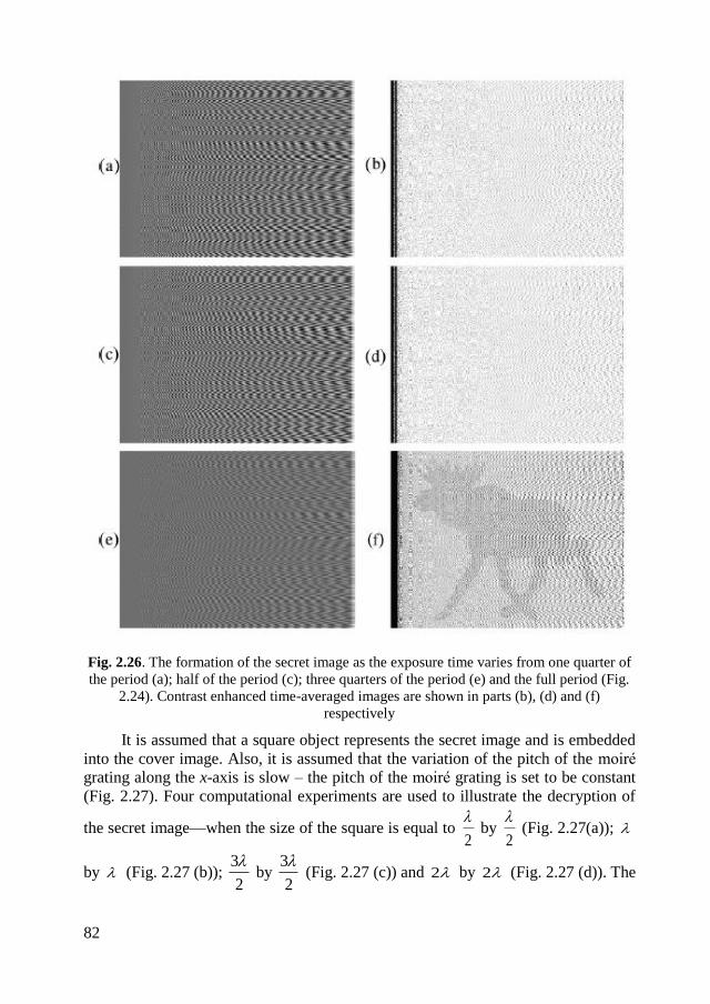
82
Fig. 2.26. The formation of the secret image as the exposure time varies from one quarter of
the period (a); half of the period (c); three quarters of the period (e) and the full period (Fig.
2.24). Contrast enhanced time-averaged images are shown in parts (b), (d) and (f)
respectively
It is assumed that a square object represents the secret image and is embedded
into the cover image. Also, it is assumed that the variation of the pitch of the moiré
grating along the x-axis is slow – the pitch of the moiré grating is set to be constant
(Fig. 2.27). Four computational experiments are used to illustrate the decryption of
the secret image—when the size of the square is equal to 2
by
2
(Fig. 2.27(a));
by (Fig. 2.27 (b)); 2
3 by
2
3 (Fig. 2.27 (c)) and 2 by 2 (Fig. 2.27 (d)). The
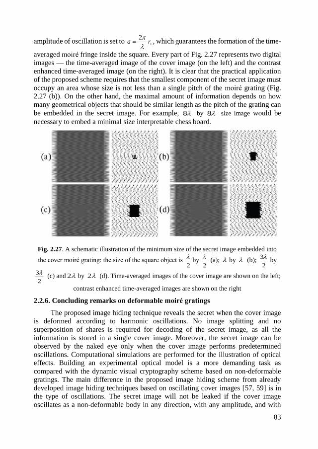
83
amplitude of oscillation is set to 1
2ra
, which guarantees the formation of the time-
averaged moiré fringe inside the square. Every part of Fig. 2.27 represents two digital
images — the time-averaged image of the cover image (on the left) and the contrast
enhanced time-averaged image (on the right). It is clear that the practical application
of the proposed scheme requires that the smallest component of the secret image must
occupy an area whose size is not less than a single pitch of the moiré grating (Fig.
2.27 (b)). On the other hand, the maximal amount of information depends on how
many geometrical objects that should be similar length as the pitch of the grating can
be embedded in the secret image. For example, 8 by 8 size image would be
necessary to embed a minimal size interpretable chess board.
Fig. 2.27. A schematic illustration of the minimum size of the secret image embedded into
the cover moiré grating: the size of the square object is 2
by
2
(a); by (b);
2
3by
2
3 (c) and 2 by 2 (d). Time-averaged images of the cover image are shown on the left;
contrast enhanced time-averaged images are shown on the right
2.2.6. Concluding remarks on deformable moiré gratings
The proposed image hiding technique reveals the secret when the cover image
is deformed according to harmonic oscillations. No image splitting and no
superposition of shares is required for decoding of the secret image, as all the
information is stored in a single cover image. Moreover, the secret image can be
observed by the naked eye only when the cover image performs predetermined
oscillations. Computational simulations are performed for the illustration of optical
effects. Building an experimental optical model is a more demanding task as
compared with the dynamic visual cryptography scheme based on non-deformable
gratings. The main difference in the proposed image hiding scheme from already
developed image hiding techniques based on oscillating cover images [57, 59] is in
the type of oscillations. The secret image will not be leaked if the cover image
oscillates as a non-deformable body in any direction, with any amplitude, and with
84
any waveform. The necessary condition for visual decoding of the secret is the
condition that the cover image must be deformed according to a predetermined
periodic law of motion. This additional mechanical operation can be considered as
additional security parameter to complement the dynamic visual cryptography key.
The principle of deformable cover image opens a completely new application area for
optical control techniques in vibrating deformable structures. The development and
practical implementation of such techniques is a definite objective of future research.
Optical applications could be implemented in micro-opto-mechanical systems, where
a stochastic cover moiré image could be formed on the surface of the cantilever. The
secret image would be leaked when the tip of the cantilever oscillated at a
predetermined amplitude (even though an optical microscope would be required to
see the secret image).
2.3. Concluding remarks
The advanced dynamic visual cryptography scheme based on near-optimal
moiré grating provides additional security of the encoded image – the secret image is
less interpretable if the cover image is oscillated harmonically. The main criterion to
optimize the moiré grating is based on the magnitude of the derivative of the standard
deviation at the amplitude corresponding to the formation of the first moiré fringe.
Evolutionary algorithms are used to find a near-optimal moiré grating that is used to
embed into cover image. All the secret information is embedded into one cover image
that serves as a ciphertext. Stochastic initial phase scrambling and phase
regularization algorithms are used to encode the secret. It is important to note that a
computer is not necessary to decode the image – a naked eye can interpret the
embedded secret as time-averaged moiré fringes if the encoded image is oscillated in
a predefined direction at predefined amplitude and according to a predefined time
function (these three conditions serve as a key).
Another advanced dynamic visual cryptography scheme based on deformable
moiré grating provides additional security level – the secret is revealed if the cover
image is harmonically deformed in a predefined direction at predefined amplitude.
Additional mechanical operation (deformation of the cover image) can be considered
as new parameter to complement the key. All the secret information is embedded into
one cover image that serves as a ciphertext. Special algorithms are used to embed the
secret. Stochastic initial phase scrambling and phase regularization algorithms are
used to encode the secret.
In spite of different type of mechanical operations that are applied for the
presented advanced dynamic visual cryptography schemes, they have one important
characteristic in common – the revealed secret image is interpreted as fully developed
moiré fringes. Does a framework for dynamic visual cryptography can be extended if
moiré fringes cannot fully develop?
85
3. CHAOTIC VISUAL CRYPTOGRAPHY
Dynamic visual cryptography schemes can be exploited for optical control of
harmonically vibrating systems [216]. But it is well known that a periodic force
applied to a nonlinear system can cause a chaotic response. A computational
framework for digital implementation of dynamic visual cryptography based on
chaotic oscillation would open new ways for practical applications. However, chaotic
oscillations do not produce fully developed time-average moiré fringes [225] and
different approach should be considered to implement dynamic visual cryptography
encryption scheme.
The construction and implementation of chaotic visual cryptography scheme,
which visualizes the secret image only when the time function determining the process
of oscillation is chaotic, is presented in chapter 3.1. Additional implementation of a
chaotic visual cryptography technique based on near-optimal moiré grating is
provided in chapter 3.2.
Secret image can only be revealed instantly in stationary regimes of oscillations,
therefore a tool for short-term time series segmentation is a necessity for an effective
experimental implementation of chaotic dynamic visual cryptography. The
construction of a short-term time series segmentation algorithm based on short-term
time series forecasting errors is presented in chapter 3.4. Short-term time series
forecasting algorithm, based on the identification of pseudo-ranks of the sequence and
internal smoothing procedure is developed in chapter 3.5.
3.1. Image hiding based on chaotic oscillations
3.1.1. Optical background and theoretical relationship
The main objective of the research, presented in this chapter, is to investigate
the feasibility of chaotic dynamic visual cryptography where the time function
determining the deflection of the encoded image from the state of equilibrium is a
Gaussian process with zero mean and pre-determined variance [226].
One-dimensional moiré grating is considered and a stepped grayscale function
is defined as follows
xxF
2sinsign5.05.0 ; (3.1)
where is the pitch of the moiré grating; the numerical value 0 corresponds to the
black color; 1 corresponds to the white color and all intermediate values correspond
to an appropriate grayscale level. F(x) can be expanded into the Fourier series Eq.
(2.10) with coefficients Eq. (2.12).
The described one-dimensional moiré grating is oscillated in the direction of the
x-axis and time-averaging optical techniques are used to register the time-averaged
image. Time-averaging operator sH describing the grayscale level of the time-
averaged image is defined in Eq. (2.14).
It is shown in [59] that if the density function xps of the time function ts
does satisfy the following requirements:
86
0xp s when sx ; xpxp ss ; Rx ; 0s (3.2)
then the time-averaged image of the moiré grating oscillated according to the time
function ts (as the exposure time T tends to infinity) reads:
sk
Pkx
bkx
aa
FxH s
k
kkss
22sin
2cos
2;
1
0 ; (3.3)
where Ps denotes the Fourier transform of the density function ps(x). The time-
averaged image can be interpreted as the convolution of the static image (the moiré
grating) and the point-spread function determining the oscillation of the original
image [227].
The main objective in this research is to construct an image hiding algorithm
based on the principles of dynamic visual cryptography [57] where the time function
describing the oscillation of the encoded image is chaotic. It means that the decryption
of the embedded secret image should be completely visual, but the decoding should
be possible only when the encoded image is oscillated chaotically. It is proved that
harmonic oscillations cannot be used for visual decryption of the secret image if it is
embedded into a stepped moiré grating due to the aperiodicity of roots of the zero
order Bessel function of the first kind [57].
It is well known that the motion of the registered object (or the registering
camera) causes the motion-induced blur [228]. Gaussian blur is one of the common
factors affecting the quality of the registered image in an optical system [229]. And
though the computational deblurring of contaminated images (and of course
computational introduction of the Gaussian blur to original images) is a well-explored
topic of research, the presented approach is different from the cryptographic point of
view. The Gaussian blur will be used to decrypt the encoded images. Since such an
approach requires the development of specialized encoding algorithms, it will be
concentrated on the effects taking place when the motion blur is caused by chaotic
oscillations. The latter fact requires detailed analysis of time-averaging processes
occurring during the Gaussian blur; such simplified approaches when contributions of
pixels outside the 3 range around the current pixel are ignored cannot be exploited
in the present computational setup.
If t is a Gaussian normal ergodic process with zero mean and 2 variance.
Then, the density function xp reads:
2
2
2exp
π2
1
xxp (3.4)
and the Fourier transform of xp takes the following form:
2
2
1exp P . (3.5)
Then, the time-averaged image of the moiré grating oscillated by a Gaussian
time function takes the following form:
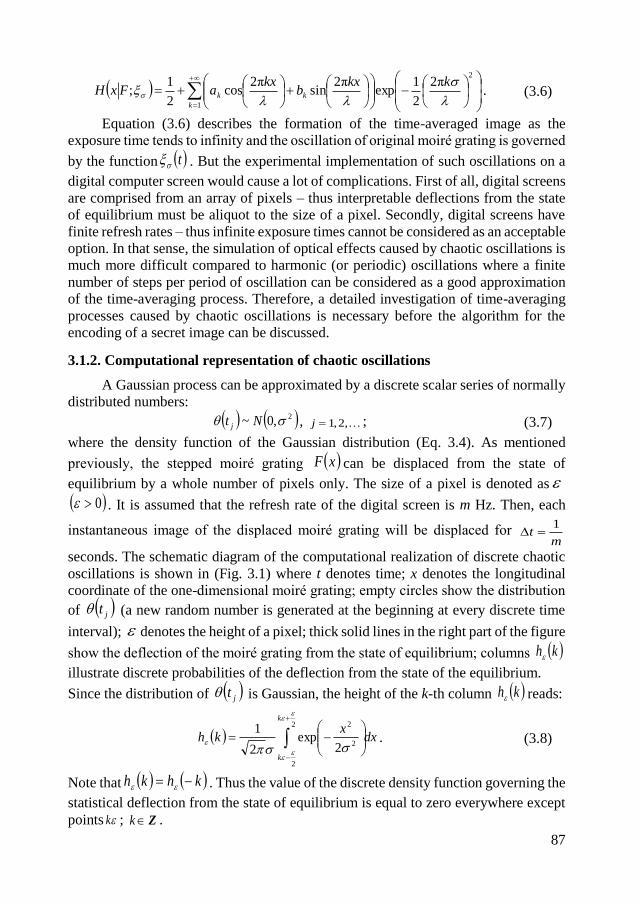
87
2
1
π2
2
1exp
π2sin
π2cos
2
1;
kkxb
kxaFxH
k
kk . (3.6)
Equation (3.6) describes the formation of the time-averaged image as the
exposure time tends to infinity and the oscillation of original moiré grating is governed
by the function t . But the experimental implementation of such oscillations on a
digital computer screen would cause a lot of complications. First of all, digital screens
are comprised from an array of pixels – thus interpretable deflections from the state
of equilibrium must be aliquot to the size of a pixel. Secondly, digital screens have
finite refresh rates – thus infinite exposure times cannot be considered as an acceptable
option. In that sense, the simulation of optical effects caused by chaotic oscillations is
much more difficult compared to harmonic (or periodic) oscillations where a finite
number of steps per period of oscillation can be considered as a good approximation
of the time-averaging process. Therefore, a detailed investigation of time-averaging
processes caused by chaotic oscillations is necessary before the algorithm for the
encoding of a secret image can be discussed.
3.1.2. Computational representation of chaotic oscillations
A Gaussian process can be approximated by a discrete scalar series of normally
distributed numbers:
2,0~ Nt j , ,2,1j ; (3.7)
where the density function of the Gaussian distribution (Eq. 3.4). As mentioned
previously, the stepped moiré grating xF can be displaced from the state of
equilibrium by a whole number of pixels only. The size of a pixel is denoted as
0 . It is assumed that the refresh rate of the digital screen is m Hz. Then, each
instantaneous image of the displaced moiré grating will be displaced for m
t1
seconds. The schematic diagram of the computational realization of discrete chaotic
oscillations is shown in (Fig. 3.1) where t denotes time; x denotes the longitudinal
coordinate of the one-dimensional moiré grating; empty circles show the distribution
of jt (a new random number is generated at the beginning at every discrete time
interval); denotes the height of a pixel; thick solid lines in the right part of the figure
show the deflection of the moiré grating from the state of equilibrium; columns kh
illustrate discrete probabilities of the deflection from the state of the equilibrium.
Since the distribution of is Gaussian, the height of the k-th column kh reads:
dxx
kh
k
k
2
2
2
2
2exp
2
1
. (3.8)
Note that khkh . Thus the value of the discrete density function governing the
statistical deflection from the state of equilibrium is equal to zero everywhere except
points ; Zk .
jt
k
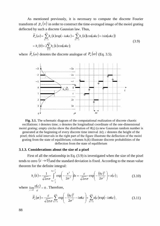
88
As mentioned previously, it is necessary to compute the discrete Fourier
transform of xp in order to construct the time-averaged image of the moiré grating
deflected by such a discrete Gaussian law. Thus,
;cos20
sincosexp~
1
kkhh
kikkhkikhP
k
kk
(3.9)
where P~
denotes the discrete analogue of P (Eq. 3.5).
Fig. 3.1. The schematic diagram of the computational realization of discrete chaotic
oscillations: t denotes time; x denotes the longitudinal coordinate of the one-dimensional
moiré grating; empty circles show the distribution of θ(tj) (a new Gaussian random number is
generated at the beginning of every discrete time interval Δt); ɛ denotes the height of the
pixel; thick solid intervals in the right part of the figure illustrate the deflection of the moiré
grating from the state of equilibrium; columns hɛ(k) illustrate discrete probabilities of the
deflection from the state of equilibrium
3.1.3. Considerations about the size of a pixel
First of all the relationship in Eq. (3.9) is investigated when the size of the pixel
tends to zero 0 and the standard deviation is fixed. According to the mean value
theorem for the definite integral:
ok
dxx
kh
k
k
2
22
2
2
2
2exp
22exp
2
1; (3.10)
where
0lim0
o. Therefore,
kk
kiokik
P
exp
2exp
2
~2
2
. (3.11)
89
But,
0limexplimexplim00
odxxi
oki
A
AA
k
, (3.12)
because 1exp ki and
dxxi
A
A
exp
(note that
Mdxxdxxdxxi
A
A
A
A
A
A
22
sincosexp for all A).
Therefore,
.2
exp
2exp
2
1
2exp
2
~lim
22
2
2
2
2
0
dxxi
xki
kP
k (3.13)
This is an important result stating that P~
converges to P as the size of a
pixel tends to zero. Nevertheless, it is important to take into account the value of
when chaotic oscillations are simulated on a particular computer display.
Alternatively, it is possible to check opposite limit when (at fixed ). It is
clear that 10lim
h and 0lim
kh
for ,2,1 k . Thus,
1explim~
lim
kikhPk
. (3.14)
All generated discrete random numbers jt will fall into the central pixel of
the stationary moiré grating if the size of the pixel is large compared to the standard
deviation . Then the moiré grating will remain stationary at the state of equilibrium
and the time-averaged image will be the image of the stationary grating (the
characteristic function modulating time-averaged fringes is equal to one then).
3.1.4. Considerations about the standard deviation
It is considered the situation when 0 (at fixed ). Now, xxp 00
lim
where
0,0
0,0
x
xx and
10 dxx . Thus,
10expexp~
lim 00
idxkixP . (3.15)
The moiré grating will not be displayed from the state of equilibrium if the
standard deviation is so small that all random numbers fall into vicinity of the
central pixel of the stationary grating.
Finally, the situation when (at fixed ) is considered. Now,
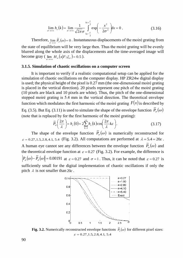
90
02
exp2
1limlim
2
2
2
2
k
k
dxx
kh . (3.16)
Therefore, 0~
lim
P . Instantaneous displacements of the moiré grating from
the state of equilibrium will be very large then. Thus the moiré grating will be evenly
blurred along the whole axis of the displacements and the time-averaged image will
become gray ( 5.0;lim
FxH ).
3.1.5. Simulation of chaotic oscillations on a computer screen
It is important to verify if a realistic computational setup can be applied for the
simulation of chaotic oscillations on the computer display. HP ZR24w digital display
is used; the physical height of the pixel is 0.27 mm (the one-dimensional moiré grating
is placed in the vertical direction). 20 pixels represent one pitch of the moiré grating
(10 pixels are black and 10 pixels are white). Thus, the pitch of the one-dimensional
stepped moiré grating is 5.4 mm in the vertical direction. The theoretical envelope
function which modulates the first harmonic of the moiré grating xF is described by
Eq. (3.5). But Eq. (3.11) is used to simulate the shape of the envelope function P~
(note that is replaced by for the first harmonic of the moiré grating):
kkhhP
k
2cos20
2~
1
. (3.17)
The shape of the envelope function P~
is numerically reconstructed for
4.5,1.4,8.2,5.1,27.0 (Fig. 3.2). All computations are performed at 204.5 .
A human eye cannot see any differences between the envelope function P~
and
the theoretical envelope function at 27.0 (Fig. 3.2). For example, the difference is
00191.0~
PP at 27.0 and 1 . Thus, it can be noted that 27.0 is
sufficiently small for the digital implementation of chaotic oscillations if only the
pitch is not smaller than 20 .
Fig. 3.2. Numerically reconstructed envelope functions P~
for different pixel sizes:
4.5,1.4,8.2,5.1,27.0
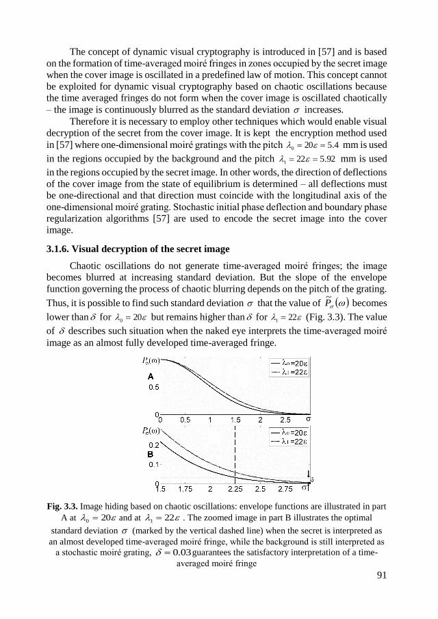
91
The concept of dynamic visual cryptography is introduced in [57] and is based
on the formation of time-averaged moiré fringes in zones occupied by the secret image
when the cover image is oscillated in a predefined law of motion. This concept cannot
be exploited for dynamic visual cryptography based on chaotic oscillations because
the time averaged fringes do not form when the cover image is oscillated chaotically
– the image is continuously blurred as the standard deviation increases.
Therefore it is necessary to employ other techniques which would enable visual
decryption of the secret from the cover image. It is kept the encryption method used
in [57] where one-dimensional moiré gratings with the pitch 4.5200 mm is used
in the regions occupied by the background and the pitch 92.5221 mm is used
in the regions occupied by the secret image. In other words, the direction of deflections
of the cover image from the state of equilibrium is determined – all deflections must
be one-directional and that direction must coincide with the longitudinal axis of the
one-dimensional moiré grating. Stochastic initial phase deflection and boundary phase
regularization algorithms [57] are used to encode the secret image into the cover
image.
3.1.6. Visual decryption of the secret image
Chaotic oscillations do not generate time-averaged moiré fringes; the image
becomes blurred at increasing standard deviation. But the slope of the envelope
function governing the process of chaotic blurring depends on the pitch of the grating.
Thus, it is possible to find such standard deviation that the value of P~
becomes
lower than for 200 but remains higher than for 221 (Fig. 3.3). The value
of describes such situation when the naked eye interprets the time-averaged moiré
image as an almost fully developed time-averaged fringe.
Fig. 3.3. Image hiding based on chaotic oscillations: envelope functions are illustrated in part
A at 200 and at 221 . The zoomed image in part B illustrates the optimal
standard deviation (marked by the vertical dashed line) when the secret is interpreted as
an almost developed time-averaged moiré fringe, while the background is still interpreted as
a stochastic moiré grating, 03.0 guarantees the satisfactory interpretation of a time-
averaged moiré fringe
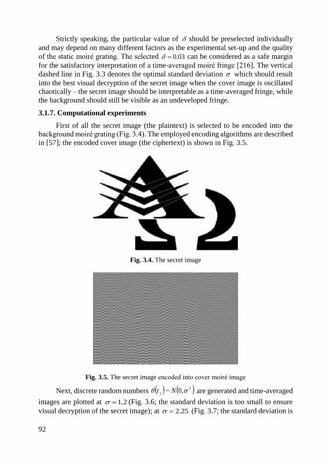
92
Strictly speaking, the particular value of should be preselected individually
and may depend on many different factors as the experimental set-up and the quality
of the static moiré grating. The selected 03.0 can be considered as a safe margin
for the satisfactory interpretation of a time-averaged moiré fringe [216]. The vertical
dashed line in Fig. 3.3 denotes the optimal standard deviation which should result
into the best visual decryption of the secret image when the cover image is oscillated
chaotically – the secret image should be interpretable as a time-averaged fringe, while
the background should still be visible as an undeveloped fringe.
3.1.7. Computational experiments
First of all the secret image (the plaintext) is selected to be encoded into the
background moiré grating (Fig. 3.4). The employed encoding algorithms are described
in [57]; the encoded cover image (the ciphertext) is shown in Fig. 3.5.
Fig. 3.4. The secret image
Fig. 3.5. The secret image encoded into cover moiré image
Next, discrete random numbers 2,0~ Nt j are generated and time-averaged
images are plotted at 2.1 (Fig. 3.6; the standard deviation is too small to ensure
visual decryption of the secret image); at 25.2 (Fig. 3.7; the standard deviation is
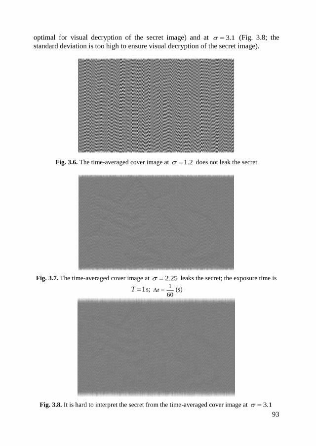
93
optimal for visual decryption of the secret image) and at 1.3 (Fig. 3.8; the
standard deviation is too high to ensure visual decryption of the secret image).
Fig. 3.6. The time-averaged cover image at 2.1 does not leak the secret
Fig. 3.7. The time-averaged cover image at 25.2 leaks the secret; the exposure time is
1T s; 60
1t (s)
Fig. 3.8. It is hard to interpret the secret from the time-averaged cover image at 1.3
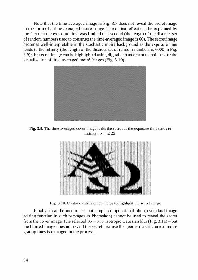
94
Note that the time-averaged image in Fig. 3.7 does not reveal the secret image
in the form of a time-averaged moiré fringe. The optical effect can be explained by
the fact that the exposure time was limited to 1 second (the length of the discreet set
of random numbers used to construct the time-averaged image is 60). The secret image
becomes well-interpretable in the stochastic moiré background as the exposure time
tends to the infinity (the length of the discreet set of random numbers is 6000 in Fig.
3.9); the secret image can be highlighted using digital enhancement techniques for the
visualization of time-averaged moiré fringes (Fig. 3.10).
Fig. 3.9. The time-averaged cover image leaks the secret as the exposure time tends to
infinity; 25.2
Fig. 3.10. Contrast enhancement helps to highlight the secret image
Finally it can be mentioned that simple computational blur (a standard image
editing function in such packages as Photoshop) cannot be used to reveal the secret
from the cover image. It is selected 75.63 isotropic Gaussian blur (Fig. 3.11) – but
the blurred image does not reveal the secret because the geometric structure of moiré
grating lines is damaged in the process.
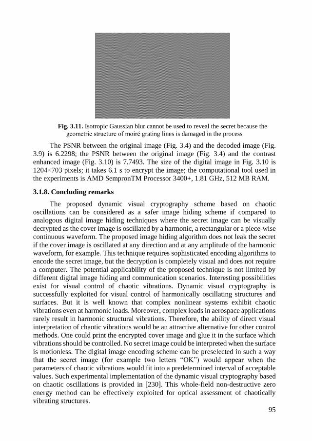
95
Fig. 3.11. Isotropic Gaussian blur cannot be used to reveal the secret because the
geometric structure of moiré grating lines is damaged in the process
The PSNR between the original image (Fig. 3.4) and the decoded image (Fig.
3.9) is 6.2298; the PSNR between the original image (Fig. 3.4) and the contrast
enhanced image (Fig. 3.10) is 7.7493. The size of the digital image in Fig. 3.10 is
1204×703 pixels; it takes 6.1 s to encrypt the image; the computational tool used in
the experiments is AMD SempronTM Processor 3400+, 1.81 GHz, 512 MB RAM.
3.1.8. Concluding remarks
The proposed dynamic visual cryptography scheme based on chaotic
oscillations can be considered as a safer image hiding scheme if compared to
analogous digital image hiding techniques where the secret image can be visually
decrypted as the cover image is oscillated by a harmonic, a rectangular or a piece-wise
continuous waveform. The proposed image hiding algorithm does not leak the secret
if the cover image is oscillated at any direction and at any amplitude of the harmonic
waveform, for example. This technique requires sophisticated encoding algorithms to
encode the secret image, but the decryption is completely visual and does not require
a computer. The potential applicability of the proposed technique is not limited by
different digital image hiding and communication scenarios. Interesting possibilities
exist for visual control of chaotic vibrations. Dynamic visual cryptography is
successfully exploited for visual control of harmonically oscillating structures and
surfaces. But it is well known that complex nonlinear systems exhibit chaotic
vibrations even at harmonic loads. Moreover, complex loads in aerospace applications
rarely result in harmonic structural vibrations. Therefore, the ability of direct visual
interpretation of chaotic vibrations would be an attractive alternative for other control
methods. One could print the encrypted cover image and glue it in the surface which
vibrations should be controlled. No secret image could be interpreted when the surface
is motionless. The digital image encoding scheme can be preselected in such a way
that the secret image (for example two letters “OK”) would appear when the
parameters of chaotic vibrations would fit into a predetermined interval of acceptable
values. Such experimental implementation of the dynamic visual cryptography based
on chaotic oscillations is provided in [230]. This whole-field non-destructive zero
energy method can be effectively exploited for optical assessment of chaotically
vibrating structures.
96
3.2. Near-optimal moiré grating for chaotic dynamic visual cryptography
It is important to note that the selection of the moiré grating and type of
oscillation must be pre-chosen before the secret image is encrypted into the cover
image. Not every moiré grating produces time-averaged fringes. It is shown in [59]
that the stepped moiré grating does not produce time-averaged moiré fringes when the
encoded image is harmonically oscillated even at appropriate amplitude and direction
of oscillations. Image hiding technique based on time-average fringes produced by
rectangular waveforms and near-optimal moiré gratings is presented chapter 2.1.
Evolutionary algorithms are used here to find near optimal moiré grating.
The main objective of this presentation is to develop a framework for chaotic
dynamic visual cryptography – it is completely unclear what types of moiré gratings
could be advantageous for chaotic oscillations. Therefore, the second objective
presented in this chapter is to identify a near-optimal moiré grating and to demonstrate
its applicability for chaotic visual cryptography.
3.2.1. Optical background and construction of the grayscale function
One-dimensional moiré grating is considered and the requirements for the
perfect grayscale function xF are provided in chapter 2.1.1. and chapter 2.1.3
(Definition 1 and Definition 6).
It is considered that m-pixels grayscale grating function knm yxF , (where x
belongs to a closed interval
j
m
kj
m
k;
1; mk ,,2,1 ; Zj and ,ky
mk ,,2,1 are grayscale levels) can be applicable for chaotic visual cryptography
presented in chapter 3.1. The size of a single pixel is m
; m pixels fit into one period
of the grayscale function.
Let us consider a situation when the described one-dimensional moiré grating is
oscillated in the direction of the x-axis and time-averaging optical techniques are used
to register the time-averaged image. Time-averaging operator sH describing the
grayscale level of the time-averaged image is defined in Eq. (2.14). It is shown in
[59] that if the density function )(xps of the time function )(ts is symmetric, then
the time-averaged image of the moiré grating reads as Eq. (3.3).
Let us require that )(t is a Gaussian normal ergodic process with zero mean
and 2 variance. The oscillation of a grayscale grating function xF nm, according to
the Gaussian time function is considered. Therefore, the standard deviation of such
time-averaged image reads:
1
2
22 2exp
2
2;
k
kkss
kbaFxHs
. (3.18)
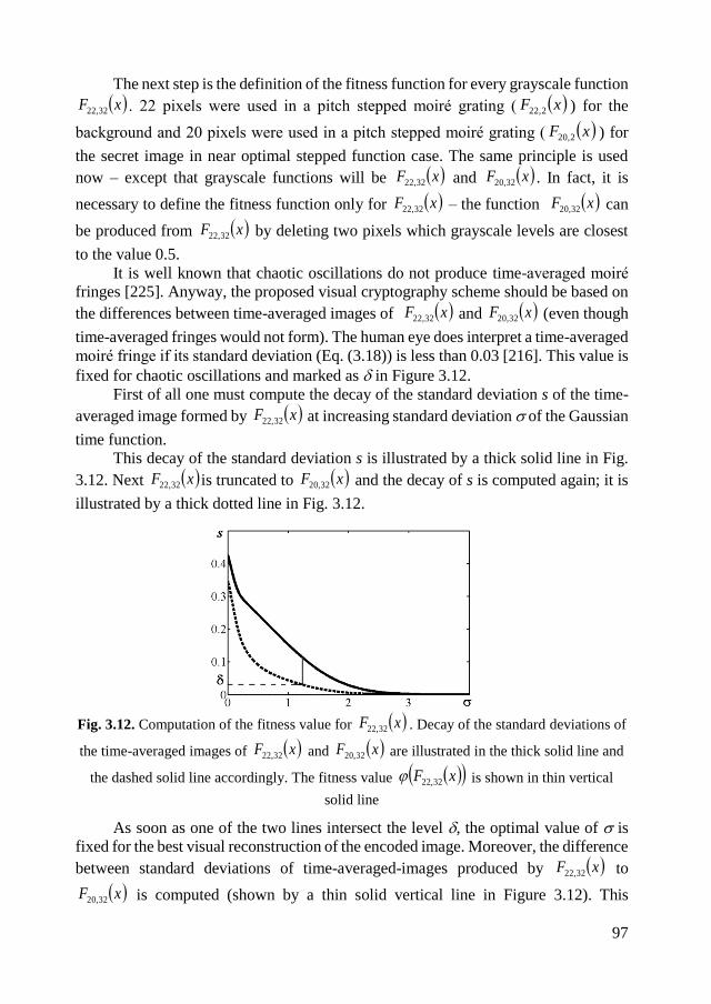
97
The next step is the definition of the fitness function for every grayscale function
xF 32,22 . 22 pixels were used in a pitch stepped moiré grating ( xF 2,22 ) for the
background and 20 pixels were used in a pitch stepped moiré grating ( xF 2,20 ) for
the secret image in near optimal stepped function case. The same principle is used
now – except that grayscale functions will be xF 32,22 and xF 32,20 . In fact, it is
necessary to define the fitness function only for xF 32,22 – the function xF 32,20 can
be produced from xF 32,22 by deleting two pixels which grayscale levels are closest
to the value 0.5.
It is well known that chaotic oscillations do not produce time-averaged moiré
fringes [225]. Anyway, the proposed visual cryptography scheme should be based on
the differences between time-averaged images of xF 32,22 and xF 32,20 (even though
time-averaged fringes would not form). The human eye does interpret a time-averaged
moiré fringe if its standard deviation (Eq. (3.18)) is less than 0.03 [216]. This value is
fixed for chaotic oscillations and marked as in Figure 3.12.
First of all one must compute the decay of the standard deviation s of the time-
averaged image formed by xF 32,22 at increasing standard deviation of the Gaussian
time function.
This decay of the standard deviation s is illustrated by a thick solid line in Fig.
3.12. Next xF 32,22 is truncated to xF 32,20 and the decay of s is computed again; it is
illustrated by a thick dotted line in Fig. 3.12.
Fig. 3.12. Computation of the fitness value for xF 32,22 . Decay of the standard deviations of
the time-averaged images of xF 32,22 and xF 32,20 are illustrated in the thick solid line and
the dashed solid line accordingly. The fitness value xF 32,22 is shown in thin vertical
solid line
As soon as one of the two lines intersect the level , the optimal value of is
fixed for the best visual reconstruction of the encoded image. Moreover, the difference
between standard deviations of time-averaged-images produced by xF 32,22 to
xF 32,20 is computed (shown by a thin solid vertical line in Figure 3.12). This
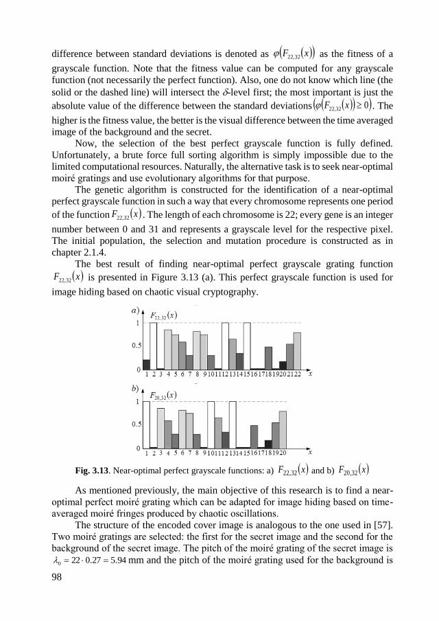
98
difference between standard deviations is denoted as xF 32,22 as the fitness of a
grayscale function. Note that the fitness value can be computed for any grayscale
function (not necessarily the perfect function). Also, one do not know which line (the
solid or the dashed line) will intersect the -level first; the most important is just the
absolute value of the difference between the standard deviations 032,22 xF . The
higher is the fitness value, the better is the visual difference between the time averaged
image of the background and the secret.
Now, the selection of the best perfect grayscale function is fully defined.
Unfortunately, a brute force full sorting algorithm is simply impossible due to the
limited computational resources. Naturally, the alternative task is to seek near-optimal
moiré gratings and use evolutionary algorithms for that purpose.
The genetic algorithm is constructed for the identification of a near-optimal
perfect grayscale function in such a way that every chromosome represents one period
of the function xF 32,22 . The length of each chromosome is 22; every gene is an integer
number between 0 and 31 and represents a grayscale level for the respective pixel.
The initial population, the selection and mutation procedure is constructed as in
chapter 2.1.4.
The best result of finding near-optimal perfect grayscale grating function
xF 32,22 is presented in Figure 3.13 (a). This perfect grayscale function is used for
image hiding based on chaotic visual cryptography.
Fig. 3.13. Near-optimal perfect grayscale functions: a) xF 32,22 and b) xF 32,20
As mentioned previously, the main objective of this research is to find a near-
optimal perfect moiré grating which can be adapted for image hiding based on time-
averaged moiré fringes produced by chaotic oscillations.
The structure of the encoded cover image is analogous to the one used in [57].
Two moiré gratings are selected: the first for the secret image and the second for the
background of the secret image. The pitch of the moiré grating of the secret image is
94.527.0220 mm and the pitch of the moiré grating used for the background is
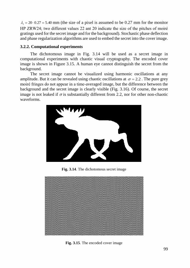
99
40.527.0201 mm (the size of a pixel is assumed to be 0.27 mm for the monitor
HP ZRW24; two different values 22 ant 20 indicate the size of the pitches of moiré
gratings used for the secret image and for the background). Stochastic phase deflection
and phase regularization algorithms are used to embed the secret into the cover image.
3.2.2. Computational experiments
The dichotomous image in Fig. 3.14 will be used as a secret image in
computational experiments with chaotic visual cryptography. The encoded cover
image is shown in Figure 3.15. A human eye cannot distinguish the secret from the
background.
The secret image cannot be visualized using harmonic oscillations at any
amplitude. But it can be revealed using chaotic oscillations at 2.2 . The pure grey
moiré fringes do not appear in a time-averaged image, but the difference between the
background and the secret image is clearly visible (Fig. 3.16). Of course, the secret
image is not leaked if is substantially different from 2.2, nor for other non-chaotic
waveforms.
Fig. 3.14. The dichotomous secret image
Fig. 3.15. The encoded cover image
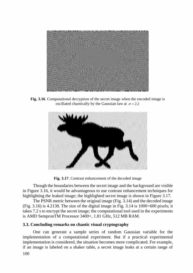
100
Fig. 3.16. Computational decryption of the secret image when the encoded image is
oscillated chaotically by the Gaussian law at 2.2
Fig. 3.17. Contrast enhancement of the decoded image
Though the boundaries between the secret image and the background are visible
in Figure 3.16, it would be advantageous to use contrast enhancement techniques for
highlighting the leaked image; the highlighted secret image is shown in Figure 3.17.
The PSNR metric between the original image (Fig. 3.14) and the decoded image
(Fig. 3.16) is 4.2138. The size of the digital image in Fig. 3.14 is 1000×600 pixels; it
takes 7.2 s to encrypt the secret image; the computational tool used in the experiments
is AMD SempronTM Processor 3400+, 1.81 GHz, 512 MB RAM.
3.3. Concluding remarks on chaotic visual cryptography
One can generate a sample series of random Gaussian variable for the
implementation of a computational experiment. But if a practical experimental
implementation is considered, the situation becomes more complicated. For example,
if an image is labeled on a shaker table, a secret image leaks at a certain range of
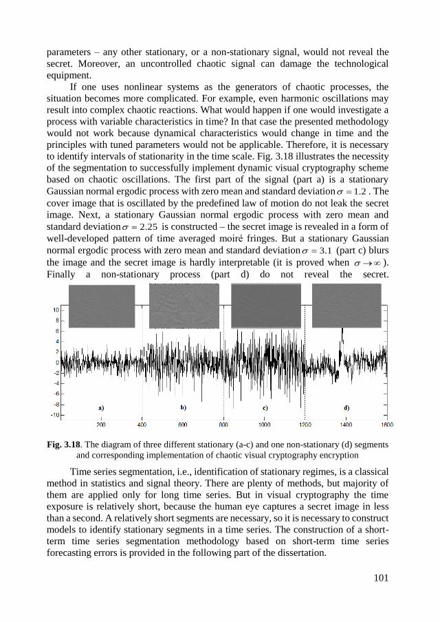
101
parameters – any other stationary, or a non-stationary signal, would not reveal the
secret. Moreover, an uncontrolled chaotic signal can damage the technological
equipment.
If one uses nonlinear systems as the generators of chaotic processes, the
situation becomes more complicated. For example, even harmonic oscillations may
result into complex chaotic reactions. What would happen if one would investigate a
process with variable characteristics in time? In that case the presented methodology
would not work because dynamical characteristics would change in time and the
principles with tuned parameters would not be applicable. Therefore, it is necessary
to identify intervals of stationarity in the time scale. Fig. 3.18 illustrates the necessity
of the segmentation to successfully implement dynamic visual cryptography scheme
based on chaotic oscillations. The first part of the signal (part a) is a stationary
Gaussian normal ergodic process with zero mean and standard deviation 2.1 . The
cover image that is oscillated by the predefined law of motion do not leak the secret
image. Next, a stationary Gaussian normal ergodic process with zero mean and
standard deviation 25.2 is constructed – the secret image is revealed in a form of
well-developed pattern of time averaged moiré fringes. But a stationary Gaussian
normal ergodic process with zero mean and standard deviation 1.3 (part c) blurs
the image and the secret image is hardly interpretable (it is proved when ).
Finally a non-stationary process (part d) do not reveal the secret.
Fig. 3.18. The diagram of three different stationary (a-c) and one non-stationary (d) segments
and corresponding implementation of chaotic visual cryptography encryption
Time series segmentation, i.e., identification of stationary regimes, is a classical
method in statistics and signal theory. There are plenty of methods, but majority of
them are applied only for long time series. But in visual cryptography the time
exposure is relatively short, because the human eye captures a secret image in less
than a second. A relatively short segments are necessary, so it is necessary to construct
models to identify stationary segments in a time series. The construction of a short-
term time series segmentation methodology based on short-term time series
forecasting errors is provided in the following part of the dissertation.
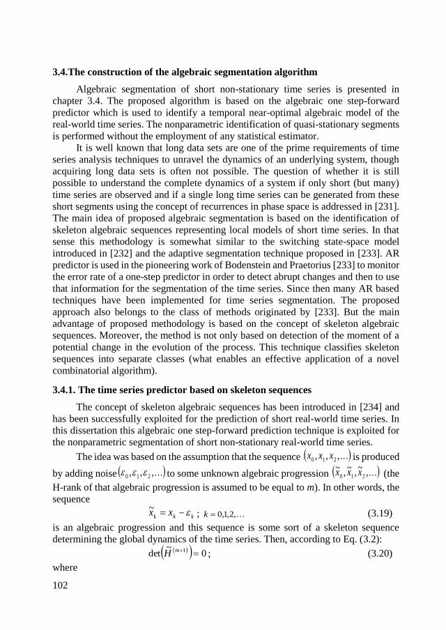
102
3.4.The construction of the algebraic segmentation algorithm
Algebraic segmentation of short non-stationary time series is presented in
chapter 3.4. The proposed algorithm is based on the algebraic one step-forward
predictor which is used to identify a temporal near-optimal algebraic model of the
real-world time series. The nonparametric identification of quasi-stationary segments
is performed without the employment of any statistical estimator.
It is well known that long data sets are one of the prime requirements of time
series analysis techniques to unravel the dynamics of an underlying system, though
acquiring long data sets is often not possible. The question of whether it is still
possible to understand the complete dynamics of a system if only short (but many)
time series are observed and if a single long time series can be generated from these
short segments using the concept of recurrences in phase space is addressed in [231].
The main idea of proposed algebraic segmentation is based on the identification of
skeleton algebraic sequences representing local models of short time series. In that
sense this methodology is somewhat similar to the switching state-space model
introduced in [232] and the adaptive segmentation technique proposed in [233]. AR
predictor is used in the pioneering work of Bodenstein and Praetorius [233] to monitor
the error rate of a one-step predictor in order to detect abrupt changes and then to use
that information for the segmentation of the time series. Since then many AR based
techniques have been implemented for time series segmentation. The proposed
approach also belongs to the class of methods originated by [233]. But the main
advantage of proposed methodology is based on the concept of skeleton algebraic
sequences. Moreover, the method is not only based on detection of the moment of a
potential change in the evolution of the process. This technique classifies skeleton
sequences into separate classes (what enables an effective application of a novel
combinatorial algorithm).
3.4.1. The time series predictor based on skeleton sequences
The concept of skeleton algebraic sequences has been introduced in [234] and
has been successfully exploited for the prediction of short real-world time series. In
this dissertation this algebraic one step-forward prediction technique is exploited for
the nonparametric segmentation of short non-stationary real-world time series.
The idea was based on the assumption that the sequence ,,, 210 xxx is produced
by adding noise ,,, 210 to some unknown algebraic progression ,~,~,~210 xxx (the
H-rank of that algebraic progression is assumed to be equal to m). In other words, the
sequence
kkk xx ~; ,2,1,0k (3.19)
is an algebraic progression and this sequence is some sort of a skeleton sequence
determining the global dynamics of the time series. Then, according to Eq. (3.2): 0
~det 1 mH ; (3.20)
where
103
mnn
m
m
m
xxx
xxx
xxx
H
21
121
10
1
~~~
~~~
~~~
~
. (3.21)
Corrections k ; mk 2,,2,1,0 had to be identified before any predictions could
be made. Since the goal was to minimize any distortions of the original time series,
the fitness function for the set of corrections m210 ,,, was introduced in [234]:
n
k
kk
n
n
Ha
F2
0
1
210~
det
1,,,
; 0a ; (3.22)
where
m
j
k
jb
kb2
0
1exp
1exp ; mk 2,,1,0 ; 0b .
(3.23)
If the original time series is an algebraic progression and
0det 1 mH , the
fitness function reaches its maximum at 0210 m ( 0,,0,0 F then).
The parameter a determines the penalty proportion between the magnitude of the
determinant and the sum of weighted corrections (both penalties have the same weight
when 1a ). Coefficients m210 ,,, determine the tolerance corridor for
corrections m210 ,,, . All corrections would have the same weight if 0b . The
larger is b, the higher is the weight for the correction of the observation at the present
moment compared to past moments. In other words, the toleration of changes for the
present moment is smaller compared to the toleration of changes for previous
moments. That corresponds to the supposition that the importance of the observation
depends on its closeness to the present moment.
It can be observed that such a prediction strategy based on the identification of
skeleton algebraic sequences and the fitness function described by Eq. (3.22) works
well for short time series and outperforms many other predictors if a day-ahead local
maximum and local minimum must to be considered. In general, the variability of the
time series forecasted by the described technique is an advantageous factor (though a
number of trials are necessary before an averaged estimate of the prediction can be
produced).
3.4.2. The artificial time series
Firstly, to validate the proposed segmentation algorithm, an artificial time series
is constructed. The artificial scalar time series comprises 191 elements (Fig. 3.19).
The first segment of the series represents a periodic sequence. The period length is 8
and elements in the period are: 0.5, 0.7, 0.1, 0.9, 0.3, 0.2, 0.8 and 0.4. The period is
repeated 6 times; the length of the first segment is 48 elements.
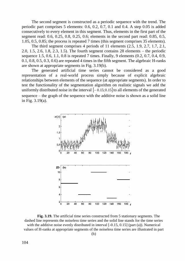
104
The second segment is constructed as a periodic sequence with the trend. The
periodic part comprises 5 elements: 0.6, 0.2, 0.7, 0.1 and 0.4. A step 0.05 is added
consecutively to every element in this segment. Thus, elements in the first part of the
segment read: 0.6, 0.25, 0.8, 0.25, 0.6; elements in the second part read: 0.85, 0.5,
1.05, 0.5, 0.85; the process is repeated 7 times (this segment comprises 35 elements).
The third segment comprises 4 periods of 11 elements (2.5, 1.9, 2.7, 1.7, 2.1,
2.0, 1.5, 2.6, 1.8, 2.3, 1.5). The fourth segment contains 28 elements – the periodic
sequence 1.5, 0.6, 1.1, 0.8 is repeated 7 times. Finally, 9 elements (0.2, 0.7, 0.4, 0.9,
0.1, 0.8, 0.5, 0.3, 0.6) are repeated 4 times in the fifth segment. The algebraic H-ranks
are shown at appropriate segments in Fig. 3.19(b).
The generated artificial time series cannot be considered as a good
representation of a real-world process simply because of explicit algebraic
relationships between elements of the sequence (at appropriate segments). In order to
test the functionality of the segmentation algorithm on realistic signals we add the
uniformly distributed noise in the interval 15.0;15.0 to all elements of the generated
sequence – the graph of the sequence with the additive noise is shown as a solid line
in Fig. 3.19(a).
Fig. 3.19. The artificial time series constructed from 5 stationary segments. The
dashed line represents the noiseless time series and the solid line stands for the time series
with the additive noise evenly distributed in interval [-0.15, 0.15] (part (a)). Numerical
values of H-ranks at appropriate segments of the noiseless time series are illustrated in part
(b)
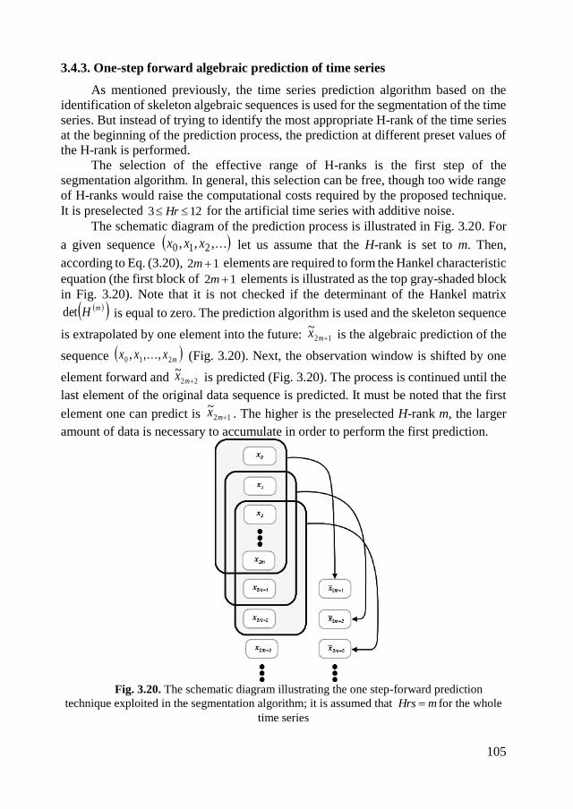
105
3.4.3. One-step forward algebraic prediction of time series
As mentioned previously, the time series prediction algorithm based on the
identification of skeleton algebraic sequences is used for the segmentation of the time
series. But instead of trying to identify the most appropriate H-rank of the time series
at the beginning of the prediction process, the prediction at different preset values of
the H-rank is performed.
The selection of the effective range of H-ranks is the first step of the
segmentation algorithm. In general, this selection can be free, though too wide range
of H-ranks would raise the computational costs required by the proposed technique.
It is preselected 123 Hr for the artificial time series with additive noise.
The schematic diagram of the prediction process is illustrated in Fig. 3.20. For
a given sequence ,,, 210 xxx let us assume that the H-rank is set to m. Then,
according to Eq. (3.20), 12 m elements are required to form the Hankel characteristic
equation (the first block of 12 m elements is illustrated as the top gray-shaded block
in Fig. 3.20). Note that it is not checked if the determinant of the Hankel matrix mHdet is equal to zero. The prediction algorithm is used and the skeleton sequence
is extrapolated by one element into the future: 12~
mx is the algebraic prediction of the
sequence mxxx 210 ,,, (Fig. 3.20). Next, the observation window is shifted by one
element forward and 22~
mx is predicted (Fig. 3.20). The process is continued until the
last element of the original data sequence is predicted. It must be noted that the first
element one can predict is 12~
mx . The higher is the preselected H-rank m, the larger
amount of data is necessary to accumulate in order to perform the first prediction.
Fig. 3.20. The schematic diagram illustrating the one step-forward prediction
technique exploited in the segmentation algorithm; it is assumed that mHrs for the whole
time series
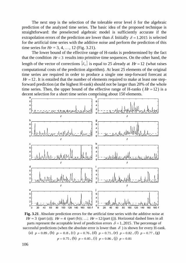
106
The next step is the selection of the tolerable error level for the algebraic
prediction of the analyzed time series. The basic idea of the proposed technique is
straightforward: the preselected algebraic model is sufficiently accurate if the
extrapolation errors of the prediction are lower than . Initially 2015.1 is selected
for the artificial time series with the additive noise and perform the prediction of this
time series for Hr = 3, 4, , 12 (Fig. 3.21).
The lower bound of the effective range of H-ranks is predetermined by the fact
that the condition 3Hr results into primitive time sequences. On the other hand, the
length of the vector of corrections k is equal to 25 already at 12Hr (what raises
computational costs of the prediction algorithm). At least 25 elements of the original
time series are required in order to produce a single one step-forward forecast at
12Hr . It is entailed that the number of elements required to make at least one step-
forward prediction (at the highest H-rank) should not be larger than 20% of the whole
time series. Then, the upper bound of the effective range of H-ranks ( 12Hr ) is a
decent selection for a short time series comprising about 150 elements.
Fig. 3.21. Absolute prediction errors for the artificial time series with the additive noise at
3Hr (part (a)); 4Hr (part (b)); …; 12Hr (part (j)). Horizontal dashed lines in all
parts represent the acceptable level of prediction errors 2015..1 . The percentage of
successful predictions (when the absolute error is lower than ) is shown for every H-rank.
(a) 89.0p , (b) 8.0p , (c) 76.0p , (d) 71.0p , (e) 82.0p , (f) 77.0p , (g)
75.0p , (h) 85.0p , (i) 86.0p , (j) 81.0p
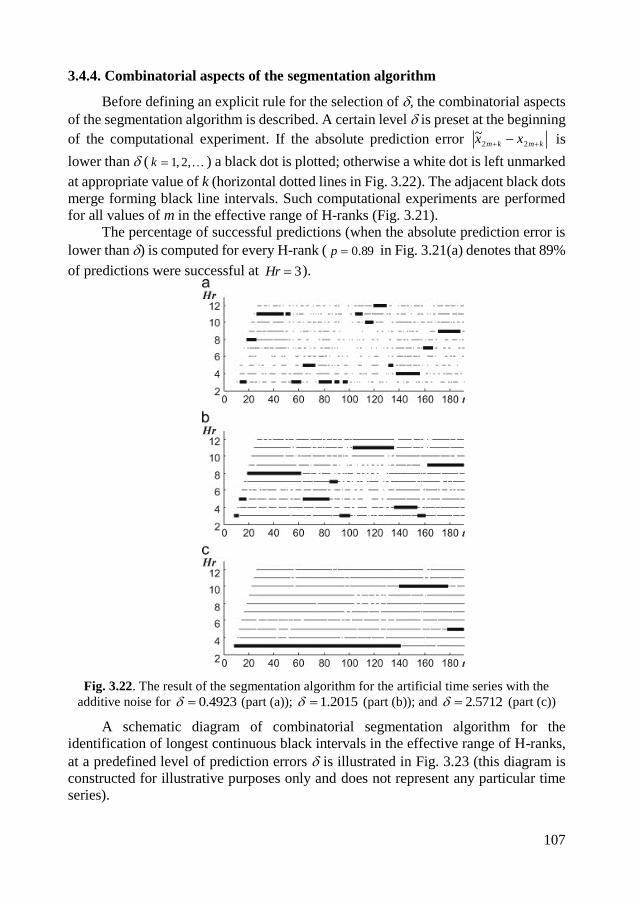
107
3.4.4. Combinatorial aspects of the segmentation algorithm
Before defining an explicit rule for the selection of , the combinatorial aspects
of the segmentation algorithm is described. A certain level is preset at the beginning
of the computational experiment. If the absolute prediction error kmkm xx 22~ is
lower than ( ,2,1k ) a black dot is plotted; otherwise a white dot is left unmarked
at appropriate value of k (horizontal dotted lines in Fig. 3.22). The adjacent black dots
merge forming black line intervals. Such computational experiments are performed
for all values of m in the effective range of H-ranks (Fig. 3.21).
The percentage of successful predictions (when the absolute prediction error is
lower than ) is computed for every H-rank ( 89.0p in Fig. 3.21(a) denotes that 89%
of predictions were successful at 3Hr ).
Fig. 3.22. The result of the segmentation algorithm for the artificial time series with the
additive noise for 4923.0 (part (a)); 2015.1 (part (b)); and 5712.2 (part (c))
A schematic diagram of combinatorial segmentation algorithm for the
identification of longest continuous black intervals in the effective range of H-ranks,
at a predefined level of prediction errors is illustrated in Fig. 3.23 (this diagram is
constructed for illustrative purposes only and does not represent any particular time
series).
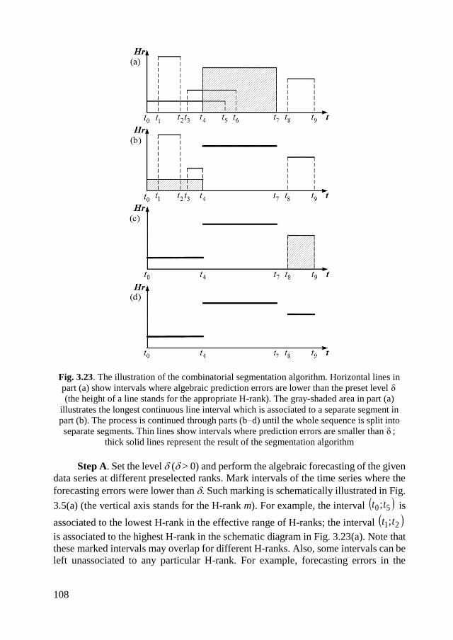
108
Fig. 3.23. The illustration of the combinatorial segmentation algorithm. Horizontal lines in
part (a) show intervals where algebraic prediction errors are lower than the preset level δ
(the height of a line stands for the appropriate H-rank). The gray-shaded area in part (a)
illustrates the longest continuous line interval which is associated to a separate segment in
part (b). The process is continued through parts (b–d) until the whole sequence is split into
separate segments. Thin lines show intervals where prediction errors are smaller than δ ;
thick solid lines represent the result of the segmentation algorithm
Step A. Set the level ( > 0) and perform the algebraic forecasting of the given
data series at different preselected ranks. Mark intervals of the time series where the
forecasting errors were lower than . Such marking is schematically illustrated in Fig.
3.5(a) (the vertical axis stands for the H-rank m). For example, the interval 50 ; tt is
associated to the lowest H-rank in the effective range of H-ranks; the interval 21;tt
is associated to the highest H-rank in the schematic diagram in Fig. 3.23(a). Note that
these marked intervals may overlap for different H-ranks. Also, some intervals can be
left unassociated to any particular H-rank. For example, forecasting errors in the
109
interval 87 ;tt are higher than for all m in the effective range of H-ranks (Fig.
3.23(a)).
Step B. Identify the longest continuous interval (in the whole range of effective
H-ranks). The longest interval 74 ;tt is marked by a gray shaded area in Fig. 3.23(a).
Step C. Denote the marked interval as the segment associated to the according
H-rank; erase all information about other H-ranks in the marked segment. The marked
segment is illustrated by a thick solid horizontal line in Fig. 3.23(b).
Step D. Identify the longest continuous interval in the zones not occupied by the
marked segments (return back to step B). The longest interval 40 ;tt is marked by a
gray shaded area in Fig. 3.23(b).
Step E. Continue until all possible intervals are marked as segments. The
interval 40 ;tt is associated to the according H-rank in Fig. 3.23(c). The last marked
interval in Fig. 3.23(c) is 98 ; tt . Finally, the segmentation algorithm identifies four
distinct segments: 40 ;tt ; 74 ;tt ; 87 ;tt and 98 ; tt in Fig 3.23(d). Note that the
unmarked interval 87 ;tt is not associated to any particular H-rank.
3.4.5. The strategy for the selection of
The results of the segmentation for the artificial time series contaminated with
noise are illustrated in Fig. 3.22 by thick solid lines. It is clear that the plotted
dichotomous lines of prediction errors in Fig. 3.22 would be sparse if is considerably
lower than the average level of absolute prediction errors (Fig. 3.22(a)). On the
contrary, continuous intervals of acceptable predictions would be long if is much
higher than the average level of absolute prediction errors (Fig. 3.22(c)). One has to
identify the appropriate level of which would result into a realistic segmentation
(Fig. 3.22(b)). Note that the darker lines in Fig. 3.22 represent the H-rank for that
segment as identified by the proposed segmentation algorithm.
The selection of the acceptable level of absolute prediction errors is illustrated
by the diagram in Fig. 3.24. As mentioned previously, the algebraic prediction of the
time series and absolute prediction errors is performed and plotted for every single H-
rank in the effective range of H-ranks. A particular level of is fixed and the
percentage of satisfactory predictions is computed in terms of (note that is the
same for all H-ranks in Fig. 3.21). Such computations are repeated for different values
of and the percentage of average satisfactory predictions p is calculated as the
arithmetic mean for all H-ranks in the effective range of H-ranks (Fig. 3.24). It is clear
that 0lim0
p
for real-world time series because the inevitable noise does not allow
the exact reconstruction of the algebraic model of the time series. On the other hand,
p saturates to 1 (corresponding to 100 %) when reaches the level of highest absolute
prediction errors (Fig. 3.24). The values 5.0p ; 0.8 and 0.95 result into 4923.0 ;
1.2015 and 2.5712 (Fig. 3.24).
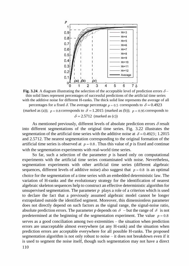
110
Fig. 3.24. A diagram illustrating the selection of the acceptable level of prediction errors –
thin solid lines represent percentages of successful predictions of the artificial time series
with the additive noise for different H-ranks. The thick solid line represents the average of all
percentages for a fixed . The average percentage 5.0p corresponds to 4923.0
(marked as (a)); 8.0p corresponds to 2015.1 (marked as (b)); 95.0p corresponds to
5712.2 (marked as (c))
As mentioned previously, different levels of absolute prediction errors result
into different segmentations of the original time series. Fig. 3.22 illustrates the
segmentation of the artificial time series with the additive noise at 4923.0 ; 1.2015
and 2.5712. The nearest segmentation corresponding to the original formation of the
artificial time series is observed at 8.0p . Thus this value of p is fixed and continue
with the segmentation experiments with real-world time series.
So far, such a selection of the parameter p is based only on computational
experiments with the artificial time series contaminated with noise. Nevertheless,
segmentation experiments with other artificial time series (different algebraic
sequences, different levels of additive noise) also suggest that 8.0p is an optimal
choice for the segmentation of a time series with an embedded deterministic law. The
variation of H-ranks and the evolutionary strategy for the identification of nearest
algebraic skeleton sequences help to construct an effective deterministic algorithm for
unsupervised segmentation. The parameter p plays a role of a criterion which is used
to declare the fact that a previously assumed algebraic model cannot be longer
extrapolated outside the identified segment. Moreover, this dimensionless parameter
does not directly depend on such factors as the signal range, the signal-noise ratio,
absolute prediction errors. The parameter p depends on – but the range of is not
predetermined at the beginning of the segmentation experiment. The value 8.0p
serves as a good conciliation among two extremities – the situation when prediction
errors are unacceptable almost everywhere (at any H-rank) and the situation when
prediction errors are acceptable everywhere for all possible H-ranks. The proposed
segmentation algorithm is not only robust to noise – it does not breakdown even if it
is used to segment the noise itself, though such segmentation may not have a direct
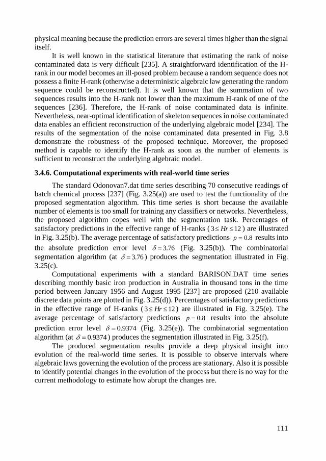
111
physical meaning because the prediction errors are several times higher than the signal
itself.
It is well known in the statistical literature that estimating the rank of noise
contaminated data is very difficult [235]. A straightforward identification of the H-
rank in our model becomes an ill-posed problem because a random sequence does not
possess a finite H-rank (otherwise a deterministic algebraic law generating the random
sequence could be reconstructed). It is well known that the summation of two
sequences results into the H-rank not lower than the maximum H-rank of one of the
sequences [236]. Therefore, the H-rank of noise contaminated data is infinite.
Nevertheless, near-optimal identification of skeleton sequences in noise contaminated
data enables an efficient reconstruction of the underlying algebraic model [234]. The
results of the segmentation of the noise contaminated data presented in Fig. 3.8
demonstrate the robustness of the proposed technique. Moreover, the proposed
method is capable to identify the H-rank as soon as the number of elements is
sufficient to reconstruct the underlying algebraic model.
3.4.6. Computational experiments with real-world time series
The standard Odonovan7.dat time series describing 70 consecutive readings of
batch chemical process [237] (Fig. 3.25(a)) are used to test the functionality of the
proposed segmentation algorithm. This time series is short because the available
number of elements is too small for training any classifiers or networks. Nevertheless,
the proposed algorithm copes well with the segmentation task. Percentages of
satisfactory predictions in the effective range of H-ranks ( 123 Hr ) are illustrated
in Fig. 3.25(b). The average percentage of satisfactory predictions 8.0p results into
the absolute prediction error level 76.3 (Fig. 3.25(b)). The combinatorial
segmentation algorithm (at 76.3 ) produces the segmentation illustrated in Fig.
3.25(c).
Computational experiments with a standard BARISON.DAT time series
describing monthly basic iron production in Australia in thousand tons in the time
period between January 1956 and August 1995 [237] are proposed (210 available
discrete data points are plotted in Fig. 3.25(d)). Percentages of satisfactory predictions
in the effective range of H-ranks ( 123 Hr ) are illustrated in Fig. 3.25(e). The
average percentage of satisfactory predictions 8.0p results into the absolute
prediction error level 9374.0 (Fig. 3.25(e)). The combinatorial segmentation
algorithm (at 9374.0 ) produces the segmentation illustrated in Fig. 3.25(f).
The produced segmentation results provide a deep physical insight into
evolution of the real-world time series. It is possible to observe intervals where
algebraic laws governing the evolution of the process are stationary. Also it is possible
to identify potential changes in the evolution of the process but there is no way for the
current methodology to estimate how abrupt the changes are.
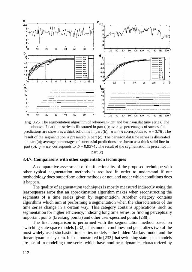
112
Fig. 3.25. The segmentation algorithm of odonovan7.dat and barinson.dat time series. The
odonovan7.dat time series is illustrated in part (a); average percentages of successful
predictions are shown as a thick solid line in part (b); 8.0p corresponds to 76.3 . The
result of the segmentation is presented in part (c). The barinson.dat time series is illustrated
in part (a); average percentages of successful predictions are shown as a thick solid line in
part (b); 8.0p corresponds to 9374.0 . The result of the segmentation is presented in
part (c)
3.4.7. Comparisons with other segmentation techniques
A comparative assessment of the functionality of the proposed technique with
other typical segmentation methods is required in order to understand if our
methodology does outperform other methods or not, and under which conditions does
it happen.
The quality of segmentation techniques is mostly measured indirectly using the
least-squares error that an approximation algorithm makes when reconstructing the
segments of a time series given by segmentation. Another category contains
algorithms which aim at performing a segmentation when the characteristics of the
time series change in a certain way. This category contains applications, such as
segmentation for higher efficiency, indexing long time series, or finding perceptually
important points (breaking points) and other user-specified points [238].
The first comparison is performed with the segmentation method based on
switching state-space models [232]. This model combines and generalizes two of the
most widely used stochastic time series models – the hidden Markov model and the
linear dynamical system. It is demonstrated in [232] that switching state-space models
are useful in modeling time series which have nonlinear dynamics characterized by
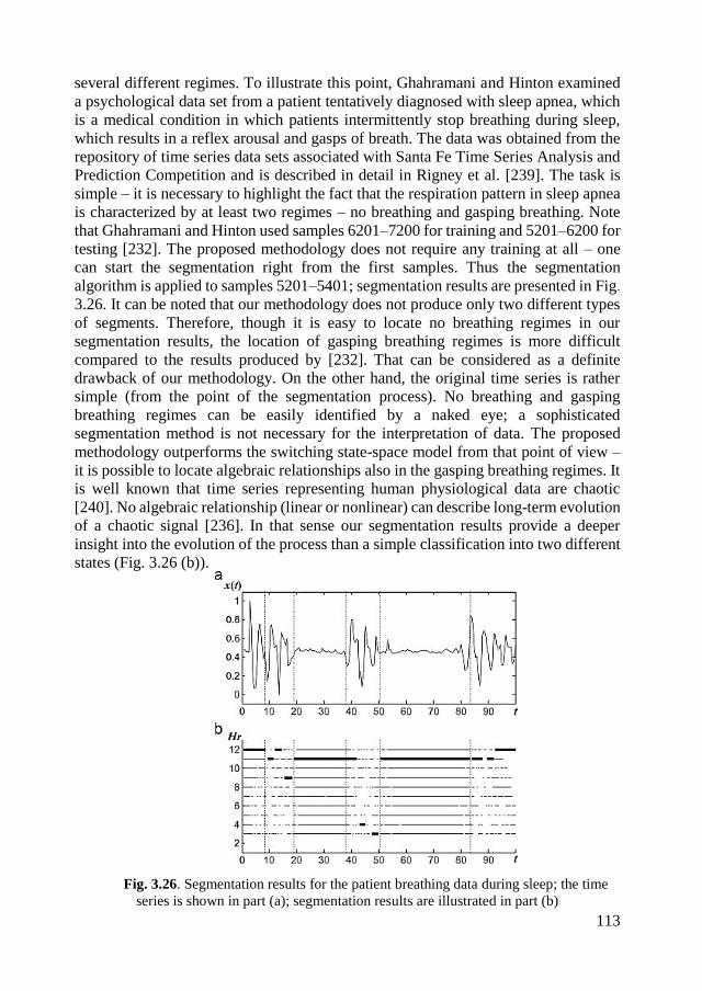
113
several different regimes. To illustrate this point, Ghahramani and Hinton examined
a psychological data set from a patient tentatively diagnosed with sleep apnea, which
is a medical condition in which patients intermittently stop breathing during sleep,
which results in a reflex arousal and gasps of breath. The data was obtained from the
repository of time series data sets associated with Santa Fe Time Series Analysis and
Prediction Competition and is described in detail in Rigney et al. [239]. The task is
simple – it is necessary to highlight the fact that the respiration pattern in sleep apnea
is characterized by at least two regimes – no breathing and gasping breathing. Note
that Ghahramani and Hinton used samples 6201–7200 for training and 5201–6200 for
testing [232]. The proposed methodology does not require any training at all – one
can start the segmentation right from the first samples. Thus the segmentation
algorithm is applied to samples 5201–5401; segmentation results are presented in Fig.
3.26. It can be noted that our methodology does not produce only two different types
of segments. Therefore, though it is easy to locate no breathing regimes in our
segmentation results, the location of gasping breathing regimes is more difficult
compared to the results produced by [232]. That can be considered as a definite
drawback of our methodology. On the other hand, the original time series is rather
simple (from the point of the segmentation process). No breathing and gasping
breathing regimes can be easily identified by a naked eye; a sophisticated
segmentation method is not necessary for the interpretation of data. The proposed
methodology outperforms the switching state-space model from that point of view –
it is possible to locate algebraic relationships also in the gasping breathing regimes. It
is well known that time series representing human physiological data are chaotic
[240]. No algebraic relationship (linear or nonlinear) can describe long-term evolution
of a chaotic signal [236]. In that sense our segmentation results provide a deeper
insight into the evolution of the process than a simple classification into two different
states (Fig. 3.26 (b)).
Fig. 3.26. Segmentation results for the patient breathing data during sleep; the time
series is shown in part (a); segmentation results are illustrated in part (b)
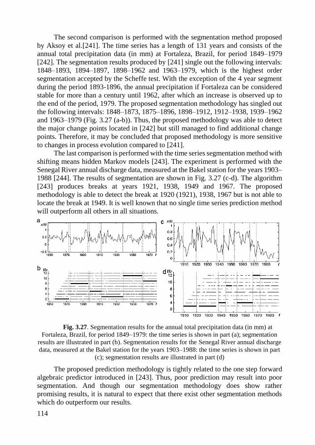
114
The second comparison is performed with the segmentation method proposed
by Aksoy et al.[241]. The time series has a length of 131 years and consists of the
annual total precipitation data (in mm) at Fortaleza, Brazil, for period 1849–1979
[242]. The segmentation results produced by [241] single out the following intervals:
1848–1893, 1894–1897, 1898–1962 and 1963–1979, which is the highest order
segmentation accepted by the Scheffe test. With the exception of the 4 year segment
during the period 1893-1896, the annual precipitation if Fortaleza can be considered
stable for more than a century until 1962, after which an increase is observed up to
the end of the period, 1979. The proposed segmentation methodology has singled out
the following intervals: 1848–1873, 1875–1896, 1898–1912, 1912–1938, 1939–1962
and 1963–1979 (Fig. 3.27 (a-b)). Thus, the proposed methodology was able to detect
the major change points located in [242] but still managed to find additional change
points. Therefore, it may be concluded that proposed methodology is more sensitive
to changes in process evolution compared to [241].
The last comparison is performed with the time series segmentation method with
shifting means hidden Markov models [243]. The experiment is performed with the
Senegal River annual discharge data, measured at the Bakel station for the years 1903–
1988 [244]. The results of segmentation are shown in Fig. 3.27 (c-d). The algorithm
[243] produces breaks at years 1921, 1938, 1949 and 1967. The proposed
methodology is able to detect the break at 1920 (1921), 1938, 1967 but is not able to
locate the break at 1949. It is well known that no single time series prediction method
will outperform all others in all situations.
Fig. 3.27. Segmentation results for the annual total precipitation data (in mm) at
Fortaleza, Brazil, for period 1849–1979: the time series is shown in part (a); segmentation
results are illustrated in part (b). Segmentation results for the Senegal River annual discharge
data, measured at the Bakel station for the years 1903–1988: the time series is shown in part
(c); segmentation results are illustrated in part (d)
The proposed prediction methodology is tightly related to the one step forward
algebraic predictor introduced in [243]. Thus, poor prediction may result into poor
segmentation. And though our segmentation methodology does show rather
promising results, it is natural to expect that there exist other segmentation methods
which do outperform our results.
115
3.4.8. Concluding remarks
It is important to note that the proposed segmentation algorithm is based on an
efficient computational strategy. Algebraic predictions are made for different H-ranks
only once. All further computations are performed with absolute prediction errors, but
the predictions do not need to be repeated. The acceptable level of prediction errors
is varied from 0 to the maximum absolute prediction error and the percentages of
successful predictions are computed for the already available data. Computations
show that the average percentage of successful predictions p=0.8 yields an optimal
value of – the optimality is considered as the closest segmentation to the underlying
intervals of quasi-stationarity.
In general, one could perform additional tuning of the parameter p – but a large
database of time series with known segmentation results should be available for that
purpose. Unfortunately, almost all available segmentation results of real world time
series are more or less empirical. Different authors compare the functionality of their
segmentation algorithms, but a “standard” segmentation cannot be found (known)
beforehand expect for an artificial time series (possibly contaminated by noise).
The proposed segmentation algorithm uses the one step-forward algebraic
predictor that is based on the concept of H-ranks. In other words, the predictor
identifies a near-optimal algebraic model of the time series and extrapolates that
model into the future. The proposed segmentation algorithm is based on the
identification of changes in the mimicking algebraic model of the time series.
The proposed algorithm belongs to the class of level-set computational
algorithms. It is not necessary to compute statistical estimators of the prediction
quality. Instead the time series are classified into dichotomous intervals according to
one step forward predictions. But instead of simply detecting the moment when
absolute prediction errors exceed a predefined level, a strategy applicable for
nonparametric identification of quasi-stationary segments is developed. It is possible
to use the same algebraic predictor and move with one step-forward forecasts until the
prediction error at some point becomes higher than a preset level. Then, one should
have to identify a new best fitting H-rank for the next interval and continue until the
prediction error exceeds the preset level again. Unfortunately, such an approach
possesses two serious drawbacks. The first one is related to the accumulation of data
before the algebraic prediction can be commenced (2m+1 data points are required for
the algebraic prediction at HrS=m). Thus, relatively long intervals between adjacent
segments would be left without an association to any segment. The second drawback
is related to a rather complex identification of the best-fitting H-rank. The proposed
strategy liberates the user from the necessity of searching a best-fitting H-rank.
Predictions are performed for all different H-ranks (in a pre-selected range) and a
combinatorial level-set based algorithm is used for the identification of appropriate
segments. Such segmentation has a deep physical meaning. The bouts of quasi-
stationarity are identified; the evolution of the process is governed by a fixed algebraic
law in each reconstructed segment. The proposed segmentation algorithm does not
apply formal algebraic relationships for the observed data. It reveals that the hidden
structure of the time series is able to identify potential changes in the evolution of the
116
process and exploits predictability as a tool for the characterization of complexity
[245].
3.5. The construction of the algebraic forecasting algorithm
Short-term time series forecasting procedures include different techniques and
models. An algebraic prediction technique based on the Hankel rank for the
identification of the skeleton algebraic sequences in short-term time series is
developed in [234]. Such an approach is used to extract information about the
algebraic model of the process and then to use this model to extrapolate past behavior
into future. It has been demonstrated in [234] that such algebraic predictor can be
effectively used for the estimation of local minimums and maximums in day-ahead
forecasting applications. It is agreeable that no single method will outperform all
others in all situations. It is shown in [234] that the proposed predictor is outperformed
(for some real-world time series) by such simple standard techniques as the moving
average or the exponential smoothing method – if only the averaged prediction errors
are considered.
The main objective of this research is to enhance the algebraic predictor
proposed in [234] by modifying the procedure for the identification of the skeleton
algebraic sequences. The main goal is to employ the procedure of internal smoothing
which should enable reaching a healthy balance between excellent variability of
skeleton algebraic sequences and valuable properties of predictors based on the
moving averaging method. The goal is to develop such a predictor which could
produce reliable forecasts for short time series that implicates skeleton algebraic
sequences – in situations when the available data is not enough for such predictors as
ARIMA or short term time series nonlinear forecasting methods such as neural
networks or support vector machines.
3.5.1. One-step forward algebraic prediction of time series
Let us assume that m2 observations are available for building a model of the
process and then using this model to extrapolate the past behavior into the future:
12210 ,,,, mxxxx ; (3.24)
where 12 mx is the value of the observation at the present moment. Let us assume that
the sequence 0; Zkxk is an algebraic progression and its H-rank is equal to m. Then
it is possible to determine the next element of the sequence mx2 from the following
equality:
0detdet
21
121
10
1
mmm
m
m
m
xxx
xxx
xxx
; (3.25)
where the only unknown is mx2 (the horizon of the prediction is equal to 1).
Unfortunately, real world series are usually contaminated with more or less noise.
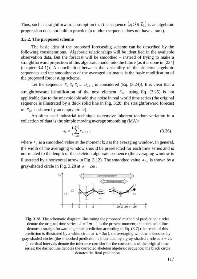
117
Thus, such a straightforward assumption that the sequence 0; Zkxk is an algebraic
progression does not hold in practice (a random sequence does not have a rank).
3.5.2. The proposed scheme
The basic idea of the proposed forecasting scheme can be described by the
following considerations. Algebraic relationships will be identified in the available
observation data. But the forecast will be smoothed – instead of trying to make a
straightforward projection of this algebraic model into the future (as it is done in [234]
(chapter 3.4.1)). A conciliation between the variability of the skeleton algebraic
sequences and the smoothness of the averaged estimates is the basic modification of
the proposed forecasting scheme.
Let the sequence 12210 ,,,, mxxxx is considered (Eq. (3.24)). It is clear that a
straightforward identification of the next element mx2 using Eq. (3.25) is not
applicable due to the unavoidable additive noise in real world time series (the original
sequence is illustrated by a thick solid line in Fig. 3.28; the straightforward forecast
of mx2 is shown by an empty circle).
An often used industrial technique to remove inherent random variation in a
collection of data is the simple moving average smoothing (MA):
1
0
1
1s
i
ikk xs
x ; (3.26)
where kx is a smoothed value at the moment k; s is the averaging window. In general,
the width of the averaging window should be preselected for each time series and is
not related to the length of the skeleton algebraic sequence (the averaging window is
illustrated by a horizontal arrow in Fig. 3.12). The smoothed value mx2 is shown by a
gray-shaded circle in Fig. 3.28 at mk 2 .
Fig. 3.28. The schematic diagram illustrating the proposed method of prediction: circles
denote the original time series; 12 mk is the present moment; the thick solid line
denotes a straightforward algebraic prediction according to Eq. (3.7) (the result of this
prediction is illustrated by a white circle at mk 2 ); the averaging window is denoted by
gray-shaded circles (the smoothed prediction is illustrated by a gray-shaded circle at mk 2
); vertical intervals denote the tolerance corridor for the corrections of the original time
series; the dashed line denotes the corrected skeleton algebraic sequence; the black circle
denotes the final prediction
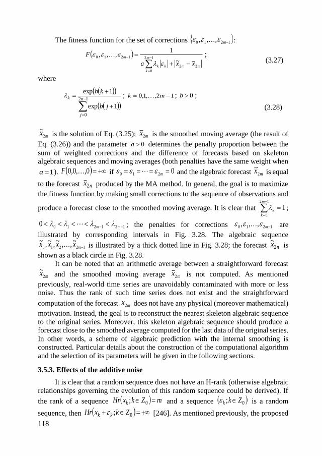
118
The fitness function for the set of corrections 1210 ,,, m :
mm
m
k
kk
m
xxa
F
22
12
0
1210
~
1,,,
; (3.27)
where
12
0
1exp
1expn
j
k
jb
kb ; 12,,1,0 mk ; 0b ;
(3.28)
mx2~
is the solution of Eq. (3.25); mx2 is the smoothed moving average (the result of
Eq. (3.26)) and the parameter 0a determines the penalty proportion between the
sum of weighted corrections and the difference of forecasts based on skeleton
algebraic sequences and moving averages (both penalties have the same weight when
1a ). 0,,0,0 F if 0210 m and the algebraic forecast mx2~
is equal
to the forecast nx2 produced by the MA method. In general, the goal is to maximize
the fitness function by making small corrections to the sequence of observations and
produce a forecast close to the smoothed moving average. It is clear that 112
0
m
k
k ;
1212100 mm ; the penalties for corrections 1210 ,,, m are
illustrated by corresponding intervals in Fig. 3.28. The algebraic sequence
12210~,,~,~,~
mxxxx is illustrated by a thick dotted line in Fig. 3.28; the forecast nx2~
is
shown as a black circle in Fig. 3.28.
It can be noted that an arithmetic average between a straightforward forecast
mx2~
and the smoothed moving average mx2 is not computed. As mentioned
previously, real-world time series are unavoidably contaminated with more or less
noise. Thus the rank of such time series does not exist and the straightforward
computation of the forecast mx2 does not have any physical (moreover mathematical)
motivation. Instead, the goal is to reconstruct the nearest skeleton algebraic sequence
to the original series. Moreover, this skeleton algebraic sequence should produce a
forecast close to the smoothed average computed for the last data of the original series.
In other words, a scheme of algebraic prediction with the internal smoothing is
constructed. Particular details about the construction of the computational algorithm
and the selection of its parameters will be given in the following sections.
3.5.3. Effects of the additive noise
It is clear that a random sequence does not have an H-rank (otherwise algebraic
relationships governing the evolution of this random sequence could be derived). If
the rank of a sequence mZkxHr k 0; and a sequence 0; Zkk is a random
sequence, then 0; ZkxHr kk [246]. As mentioned previously, the proposed
119
forecasting method is based on the identification of underlying skeleton algebraic
progression in real-world time series contaminated by the inherent noise.
The concept of the pseudospectrum of a square matrix is thoroughly investigated
in [246]. Analogous reasoning in regards to pseudo H-rank could help to understand
the effects introduced by the additive noise to the underlying algebraic relationships
governing the evolution of sequences (even though the H-rank of the sequence with
the additive noise does not exist).
The spectrum of a square matrix A, denoted as A , is the set of Cz where
the resolvent 1 AzI does not exist or is unbounded [247] (I is the identity matrix).
For each 0 , the -pseudospectrum of A is defined by [247]:
EEEAzzA with somefor :C . (3.29)
In analogy to the classical definition of the spectrum of a square matrix the H-
spectrum of the base fragment of the algebraic progression is defined as the set of
characteristic roots k of the characteristic equation. Then, for each 0 , the -H-
pseudospectrum is the subset on the complex plane comprising all possible locations
of characteristic roots of the perturbed original sequence:
.
12,,2,1 ; ;,,, with
,,, somefor ,,,:
,,,
21210
121012121100
1210
mk
xxxzz
xxx
km
mmm
m
R
C
(3.30)
There is a principal difference between Eq. (3.29) and Eq. (3.30) – the Hankel
matrix is not perturbed, but the elements of the base fragment of the algebraic
progression instead (the motivation can be explained by the fact what the extrapolation
of the sequence is explored). Moreover, the conflict associated to the nonexistence of
the H-rank of the algebraic progression contaminated with additive noise is avoided.
The element mx2 is not defined (and do not perturbed). This element can be solved
from the equation 01 md . Thus the H-rank of the perturbed sequence remains
equal to the H-rank of the unperturbed sequence. Another difference is based on the
fact that the perturbing matrix E in the classical definition of the pseudospectrum
comprises complex numbers while the perturbing vector comprising real numbers
only is employed. As mentioned previously, this can be explained by the fact that real
time series are extrapolated only.
The computation of the -H-pseudospectrum requires finding roots of the
perturbed characteristic equation (Eq. (1.26)). The m roots of the polynomial of degree
m depend continuously on the coefficients (though the problem of approximating the
roots given the coefficients is ill-conditioned). The coefficients of the polynomial are
appropriate adjuncts of the determinant. But
21detdetdet OEAtrAAEA . (3.31)
Thus, following properties hold for a small perturbation of the base fragment of
the algebraic progression in the described computational setup:
it does not change the H-rank of the sequence;
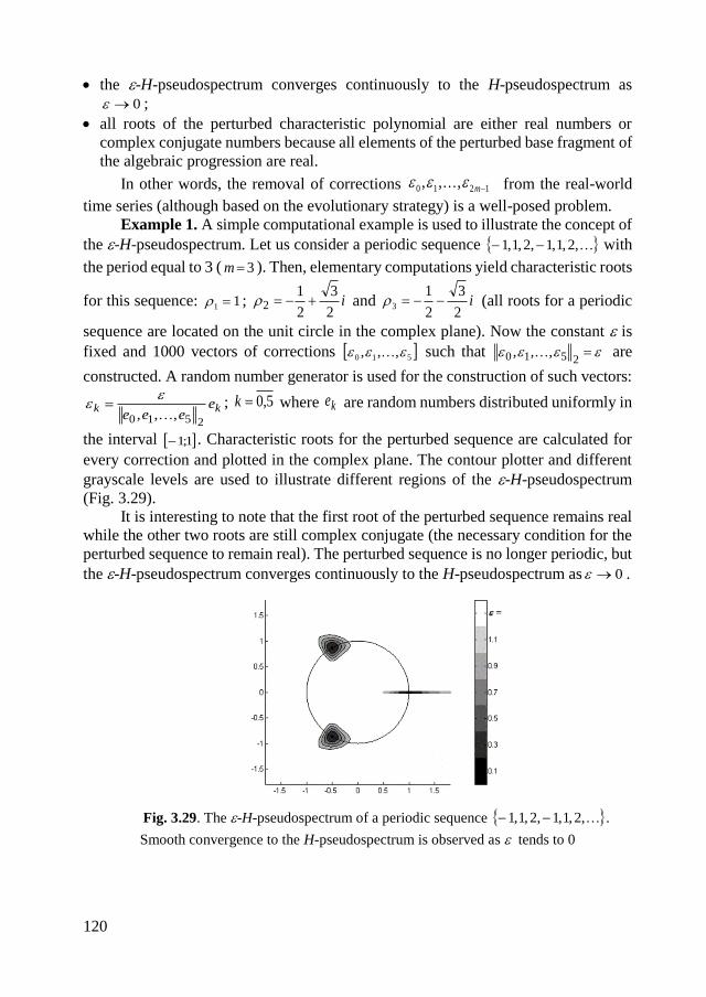
120
the -H-pseudospectrum converges continuously to the H-pseudospectrum as
0 ;
all roots of the perturbed characteristic polynomial are either real numbers or
complex conjugate numbers because all elements of the perturbed base fragment of
the algebraic progression are real.
In other words, the removal of corrections 1210 ,,, m from the real-world
time series (although based on the evolutionary strategy) is a well-posed problem.
Example 1. A simple computational example is used to illustrate the concept of
the -H-pseudospectrum. Let us consider a periodic sequence ,2,1,1,2,1,1 with
the period equal to 3 ( 3m ). Then, elementary computations yield characteristic roots
for this sequence: 11 ; i2
3
2
12 and i
2
3
2
13 (all roots for a periodic
sequence are located on the unit circle in the complex plane). Now the constant is
fixed and 1000 vectors of corrections 510 ,,, such that 2510 ,,, are
constructed. A random number generator is used for the construction of such vectors:
kk eeee
2510 ,,,
; 5,0k where ke are random numbers distributed uniformly in
the interval 1;1 . Characteristic roots for the perturbed sequence are calculated for
every correction and plotted in the complex plane. The contour plotter and different
grayscale levels are used to illustrate different regions of the -H-pseudospectrum
(Fig. 3.29).
It is interesting to note that the first root of the perturbed sequence remains real
while the other two roots are still complex conjugate (the necessary condition for the
perturbed sequence to remain real). The perturbed sequence is no longer periodic, but
the -H-pseudospectrum converges continuously to the H-pseudospectrum as 0 .
Fig. 3.29. The -H-pseudospectrum of a periodic sequence ,2,1,1,2,1,1 .
Smooth convergence to the H-pseudospectrum is observed as tends to 0
121
3.5.4. A simple numerical example
Let the concept of the proposed forecasting scheme is illustrated by a simple
numerical example. Let four observations are available: 10 x ; 21 x ; 02 x and
23 x . Let the averaging window 2s ; then the smoothed prediction is 14 x . The
straightforward algebraic forecast is 14 x because 0
120
202
021
. For the
simplicity it is assumed that 1a and 0b . Then it is necessary to find such
corrections k ; 3,2,1,0k that maximize the value of the fitness function defined by
Eq. (3.9). Eq. (3.7) yields the value of the algebraic forecast:
2120
1230322312
421
221222~
x .
(3.32)
It is necessary to determine such values of k ; 3,2,1,0k that the value of the
fitness function 3210 ,,, F is optimal. The lowest bound of the fitness function is
5.0~1
0,,0,022
mm xx
F . But the selection of the optimal corrections k ;
3,2,1,0k is not a trivial task even for this simple example. The situation would
become much more complex in case of realistic prediction scenarios. Therefore the
development of a reliable and an efficient optimization strategy becomes a subject of
the primary importance for the successful implementation of such a forecasting
strategy.
3.5.5. Parameter selection in PSO
It is clear that the prediction of an algebraic sequence by the proposed algebraic
forecasting method with internal smoothing cannot be exact. The direct computation
of the “forecast” using Eq. (3.25) is of course analytic (i.e. exact). But the fitness
function in Eq. (3.27) does not comprise a term representing the determinant of the
Hankel matrix. In other words, the exact forecast of an exact algebraic sequence is
impossible because the value of the forecast can be far from the smoothed average
(note that the exact prediction of an algebraic sequence works well with the fitness
function in Eq. (3.27)). As mentioned previously, there does not exist one method
which would outperform all others, in all situations. It is natural to expect that the
proposed method should work well with such signals where the noise – signal ratio is
rather high.
An artificial test time series to tune parameters of the proposed forecasting
algorithm and a periodic sequence is formed (numerical values of seven elements in
a period are selected as 0.5; 0.7; 0.1; 0.9; 0.3; 0.2; 0.8); this sequence represents a
skeleton algebraic sequence. Random numbers uniformly distributed in the interval
122
15.0;15.0 are added to all elements of that sequence. This test time series will be
used for testing the functionality of the proposed method.
The first task is to identify the H-rank of the time series (incorrect identification
of an appropriate H-rank may lead to substantial prediction errors). Eq. (3.25) is used
to solve mx2~
without using any corrections or moving averages ( mx2~
does not
necessarily coincide with mx2 ). Then the observation window is shifted by one
element forward and again use Eq. (3.25) to solve the next element 12~
mx . Such direct
one-step forward forecasting is repeated for 50 times; root mean square errors (RMSE)
of such direct algebraic prediction are shown in Table 3.1. Best results are produced
at 7m (the dimension of the characteristic Hankel matrix is 8), thus it is assumed
that the H-rank of the test time series is 7.
Table 3.1. RMSE of the direct algebraic prediction for the test time series at
different m m 4 5 6 7 8
RMSE 1.2960 2.1512 21.5646 0.1967 28.7332
9 10 11 12 13 14
1.0214 3.4570 18.4699 7.2924 18.4942 1.3620
The averaging window s for the simple moving average smoothing (Eq. (3.26))
and the penalty proportion parameter a must be selected in the next step (the parameter
b is set to 0). The test time series will be used again, but evolutionary algorithms will
be used now to identify the near-optimal the set of corrections 1310 ,,, .
Particle swarm optimization (PSO) techniques have been successfully employed
in [234] for the identification of the skeleton algebraic sequence. In this research PSO
are also used for the selection of a near-optimal set of corrections. And though despite
numerous research efforts the selection of the parameters of PSO remains mostly
empirical and depends on the topology of the target function and/or on the structure
of the fitness function, it is fixed 6.0w and 7.121 cc as recommended by Trelea
[189] ( 1c and 2c are two positive constants, called acceleration constants,
representing weightings of the stochastic acceleration terms that pull each particle
toward the particle’s best and the global best; w is the inertia weight balancing the
global and the local search). There have been no definitive recommendations in the
literature regarding the swarm size in PSO. Eberhart and Shi [177] indicated that the
effect of the population size on the performance of the PSO method is of minimum
significance. Most researchers use a swarm size of 10 to 60, but there are no
established guidelines. For the purpose of comparing the efficiency of the predictor
developed in [234] and the proposed method, the swarm size that is used for PSO is
fixed to 50 particles.
It is clear that a new set of near-optimal corrections 1210 ,,, m is generated
every time when the PSO algorithm is executed. Thus the PSO algorithm is executed
100 times, compute the forecasted value of mx2~
(100 different estimates of mx2~
are
produced in the process) and calculate root mean square errors (RMSE) between the
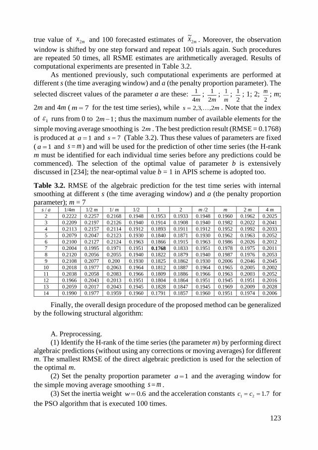
123
true value of mx2 and 100 forecasted estimates of mx2~
. Moreover, the observation
window is shifted by one step forward and repeat 100 trials again. Such procedures
are repeated 50 times, all RSME estimates are arithmetically averaged. Results of
computational experiments are presented in Table 3.2.
As mentioned previously, such computational experiments are performed at
different s (the time averaging window) and a (the penalty proportion parameter). The
selected discreet values of the parameter a are these: m4
1;
m2
1;
m
1;
2
1; 1; 2;
2
m; m;
2m and 4m ( 7m for the test time series), while ms 2,,3,2 . Note that the index
of k runs from 0 to 12 m ; thus the maximum number of available elements for the
simple moving average smoothing is m2 . The best prediction result (RMSE = 0.1768)
is produced at 1a and 7s (Table 3.2). Thus these values of parameters are fixed
( 1a and ms ) and will be used for the prediction of other time series (the H-rank
m must be identified for each individual time series before any predictions could be
commenced). The selection of the optimal value of parameter b is extensively
discussed in [234]; the near-optimal value b = 1 in APIS scheme is adopted too.
Table 3.2. RMSE of the algebraic prediction for the test time series with internal
smoothing at different s (the time averaging window) and a (the penalty proportion
parameter); m = 7 s / a 1/4m 1/2 m 1/ m 1/2 1 2 m /2 m 2 m 4 m
2 0.2222 0.2257 0.2168 0.1948 0.1953 0.1933 0.1948 0.1960 0.1962 0.2025
3 0.2209 0.2197 0.2126 0.1940 0.1914 0.1908 0.1940 0.1982 0.2022 0.2041
4 0.2113 0.2157 0.2114 0.1912 0.1893 0.1911 0.1912 0.1952 0.1992 0.2033
5 0.2079 0.2047 0.2123 0.1930 0.1840 0.1871 0.1930 0.1962 0.1963 0.2052
6 0.2100 0.2127 0.2124 0.1963 0.1866 0.1915 0.1963 0.1986 0.2026 0.2012
7 0.2004 0.1995 0.1971 0.1951 0.1768 0.1833 0.1951 0.1978 0.1975 0.2011
8 0.2120 0.2056 0.2055 0.1940 0.1822 0.1879 0.1940 0.1987 0.1976 0.2053
9 0.2108 0.2077 0.200 0.1930 0.1825 0.1862 0.1930 0.2006 0.2046 0.2045
10 0.2018 0.1977 0.2063 0.1964 0.1812 0.1887 0.1964 0.1965 0.2005 0.2002
11 0.2038 0.2058 0.2083 0.1966 0.1809 0.1886 0.1966 0.1963 0.2003 0.2052
12 0.1966 0.2043 0.2013 0.1951 0.1804 0.1864 0.1951 0.1945 0.1951 0.2016
13 0.2059 0.2017 0.2043 0.1945 0.1828 0.1847 0.1945 0.1969 0.2009 0.2028
14 0.1990 0.1977 0.1959 0.1960 0.1791 0.1857 0.1960 0.1951 0.1974 0.2006
Finally, the overall design procedure of the proposed method can be generalized
by the following structural algorithm:
A. Preprocessing.
(1) Identify the H-rank of the time series (the parameter m) by performing direct
algebraic predictions (without using any corrections or moving averages) for different
m. The smallest RMSE of the direct algebraic prediction is used for the selection of
the optimal m.
(2) Set the penalty proportion parameter 1a and the averaging window for
the simple moving average smoothing ms .
(3) Set the inertia weight 6.0w and the acceleration constants 7.121 cc for
the PSO algorithm that is executed 100 times.
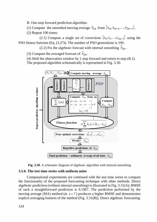
124
B. One-step forward prediction algorithm.
(1) Compute the smoothed moving average mx2 from 121 ,,, mmm xxx .
(2) Repeat 100 times:
(2.1) Compute a single set of corrections 1210 ,,, m using the
PSO fitness function (Eq. (3.27)). The number of PSO generations is 100.
(2.2) Fix the algebraic forecast with internal smoothing mx2~
.
(3) Compute the averaged forecast of mx2~
.
(4) Shift the observation window by 1 step forward and return to step (B.1).
The proposed algorithm schematically is represented in Fig. 3.30.
Fig. 3.30. A schematic diagram of algebraic algorithm with internal smoothing
3.5.6. The test time series with uniform noise
Computational experiments are continued with the test time series to compare
the functionality of the proposed forecasting technique with other methods. Direct
algebraic prediction (without internal smoothing) is illustrated in Fig. 3.31(A); RMSE
of such a straightforward prediction is 0.1967. The prediction performed by the
moving average (MA) method (at 7s ) produces a higher RMSE and demonstrates
explicit averaging features of the method (Fig. 3.31(B)). Direct algebraic forecasting
125
already outperforms MA if RMSE metrics would be considered only. But the
variability of the predicted time series is incomparably better in Fig. 3.31(A) than in
Fig. 3.31(B) (though some overestimates of local minima and local maxima can be
observed in Fig. 3.31(A)). Algebraic prediction with internal smoothing (APIS)
produces the best RMSE and the best estimates of local extremes for the test time
series (Fig. 3.31(C)). Local fluctuations of the predicted time series by our method
give a much better representation of the variability of the time series. For instance,
our method would clearly outperform the MA method if one would be interested to
identify a day-ahead local maxima and local minima. The conciliation of powerful
algebraic variability and the smoothness of moving averaging helps to unleash the
power of the proposed technique.
A prediction method based on the identification of algebraic skeleton sequences
is developed in [234]. The one-step-forward forecast of this method is constructed as
an arithmetic average of successful trials – thus this prediction method can be denoted
as the algebraic prediction with external smoothing (APES) in Fig. 3.31(D). By the
way it is used the same test series as in [234]; RMSE of APES prediction is slightly
higher compared to APIS prediction. As mentioned previously, RMSE is the only one
indicator describing the quality of the predicted time series. APES produces worse
estimates of the day-ahead local maximums and local minimums compared to the
APIS forecast (Fig. 3.31).
The functionality of APIS is compared with the predictor based on sequential
exponential smoothing (SES) which is an often used industrial technique to remove
inherent random variation in a collection of data. It is a simple and pragmatic approach
to forecasting, whereby the forecast is constructed from an exponentially weighted
average of past observations. Series of computational experiments are performed to
identify the best value (in terms of RMSE) for the test time series – best results are
produced at 1.0 . The test series does not contain a clearly expressed trend or
seasonality, therefore computational experiments are run with a SES only. The
produced RMSE is 0.2832; the results are presented in Fig. 3.31(E).
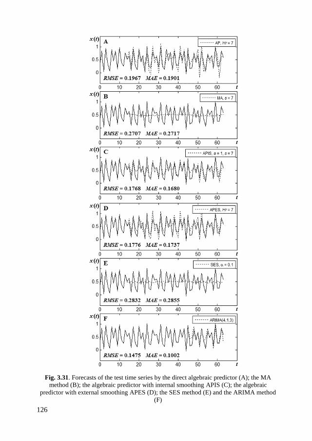
126
Fig. 3.31. Forecasts of the test time series by the direct algebraic predictor (A); the MA
method (B); the algebraic predictor with internal smoothing APIS (C); the algebraic
predictor with external smoothing APES (D); the SES method (E) and the ARIMA method
(F)
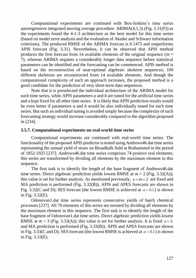
127
Computational experiments are continued with Box-Jenkins’s time series
autoregressive integrated moving average procedure ARIMA(4,1,3) (Fig. 3.31(F)) as
the experiments found the 4-1-3 architecture as the best model for this time series
(based on model error analysis and the evaluation of Akaike and Schwarz information
criterions). The produced RMSE of the ARIMA forecast is 0.1475 and outperforms
APIS forecast (Fig. 3.31). Nevertheless, it can be observed that APIS method
produces the first forecast from 14 available elements of the original sequence (m =
7), whereas ARIMA requires a considerably longer data sequence before statistical
parameters can be identified and the forecasting can be commenced. APIS method is
based on the reconstruction of near-optimal algebraic skeleton sequences; 100
different skeletons are reconstructed from 14 available elements. And though the
computational complexity of such an approach increases, the proposed method is a
good candidate for the prediction of very short-term data sequences.
Note that it is preselected the individual architecture of the ARIMA model for
each time series, while APIS parameters a and b are tuned for the artificial time series
and a kept fixed for all other time series. It is likely that APIS prediction results would
be even better if parameters a and b would be also individually tuned for each time
series. But such an individual tuning is avoided simply because the complexity of such
forecasting strategy would increase considerably compared to the algorithm proposed
in [234].
3.5.7. Computational experiments on real-world time series
Computational experiments are continued with real-world time series. The
functionality of the proposed APIS predictor is tested using Andrews46.dat time series
representing the annual yield of straw on Broadbalk field at Rothamsted in the period
of 1852-1925 [237]. Andrews46.dat time series comprises 74 positive real elements;
this series are transformed by dividing all elements by the maximum element in this
sequence.
The first task is to identify the length of the base fragment of Andrews46.dat
time series. Direct algebraic prediction yields lowest RMSE at m = 2 (Fig. 3.32(A));
this value is set for further analysis. As mentioned previously, 2ms are fixed and
MA prediction is performed (Fig. 3.32(B)). APIS and APES forecasts are shown in
Fig. 3.32(C and D); SES forecast (the lowest RMSE is achieved at 1.0 ) is shown
in Fig. 3.32(E).
Odonovan1.dat time series represents consecutive yields of batch chemical
processes [237]. All 70 elements of this series are normed by dividing all elements by
the maximum element in this sequence. The first task is to identify the length of the
base fragment of Odonovan1.dat time series. Direct algebraic prediction yields lowest
RMSE at m = 3 (Fig. 3.33(A)); this value is set for further analysis. It is fixed 3s
and MA prediction is performed (Fig. 3.33(B)). APIS and APES forecasts are shown
in Fig. 3.33(C and D); SES forecast (the lowest RMSE is achieved at 1.0 ) is shown
in Fig. 3.33(E).
128
Fig. 3.32. Forecasts of Andrews46.dat time series by the direct algebraic predictor (A); the
MA method (B); the APIS method (C); the APES method (D); the SES method (E) and the
ARIMA method (F)

129
Fig. 3.33. Forecasts of Odonovan1.dat time series by the direct algebraic predictor (A); the
MA method (B); the APIS method (C); the APES method (D); the SES method (E) and the
ARIMA method (F)
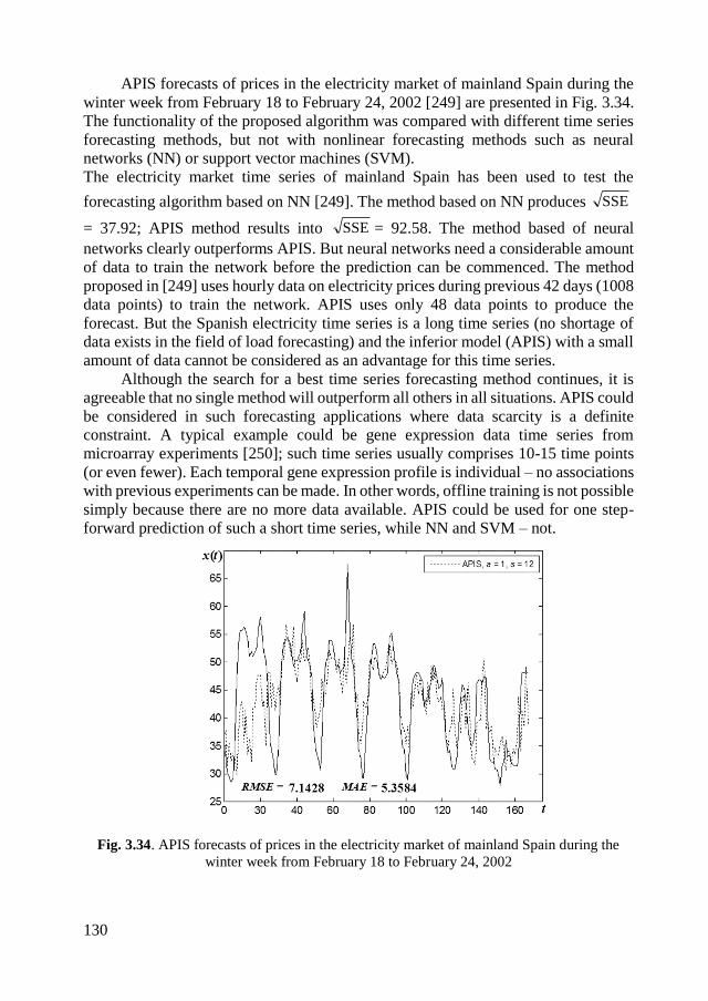
130
APIS forecasts of prices in the electricity market of mainland Spain during the
winter week from February 18 to February 24, 2002 [249] are presented in Fig. 3.34.
The functionality of the proposed algorithm was compared with different time series
forecasting methods, but not with nonlinear forecasting methods such as neural
networks (NN) or support vector machines (SVM).
The electricity market time series of mainland Spain has been used to test the
forecasting algorithm based on NN [249]. The method based on NN produces SSE
= 37.92; APIS method results into SSE = 92.58. The method based of neural
networks clearly outperforms APIS. But neural networks need a considerable amount
of data to train the network before the prediction can be commenced. The method
proposed in [249] uses hourly data on electricity prices during previous 42 days (1008
data points) to train the network. APIS uses only 48 data points to produce the
forecast. But the Spanish electricity time series is a long time series (no shortage of
data exists in the field of load forecasting) and the inferior model (APIS) with a small
amount of data cannot be considered as an advantage for this time series.
Although the search for a best time series forecasting method continues, it is
agreeable that no single method will outperform all others in all situations. APIS could
be considered in such forecasting applications where data scarcity is a definite
constraint. A typical example could be gene expression data time series from
microarray experiments [250]; such time series usually comprises 10-15 time points
(or even fewer). Each temporal gene expression profile is individual – no associations
with previous experiments can be made. In other words, offline training is not possible
simply because there are no more data available. APIS could be used for one step-
forward prediction of such a short time series, while NN and SVM – not.
Fig. 3.34. APIS forecasts of prices in the electricity market of mainland Spain during the
winter week from February 18 to February 24, 2002
131
The proposed forecasting method is based on the identification of a near-optimal
set of corrections, the reconstruction of the algebraic model of the time series and the
extrapolation this model into the future. The identification of corrections is performed
using PSO algorithms. A single run may not guarantee the repeatability and
reproducibility of results since PSO is a stochastic optimization method. It is tried to
avoid random deflections and average 100 trials for the same data set. Such averaging
enables to smooth random deflections and helps to achieve the reproducibility of
results.
3.5.8. Concluding remarks
A method for a short-term time series algebraic forecasting with internal
smoothing is proposed in this section. It is based on the identification of skeleton
algebraic sequences and finds a near-optimal balance between algebraic variability
and the smoothness of moving averages. The proposed method is especially effective
when the time series is short and there are not sufficient data to train models based on
neural or fuzzy networks.
So far, the parameters of the proposed forecasting algorithm (the penalty
proportion between the magnitude of the determinant and the sum of weighted
corrections a and the averaging window s) based on the computational experiments
with the artificial time series are tuned; these values of parameters were used to
forecast real-world time series also. One could expect even better results if the
parameters a and s would be individually tuned for every time series.
On the other hand, it is quite probable that the forecasting accuracy of the
proposed method can be improved by the introduction of variable lengths of base
fragments at different locations of the forecasted time series. Such computational
procedure is directly related to the segmentation of the time series and such adaptive
identification of the skeleton algebraic sequences remains a definite target of the
future research.
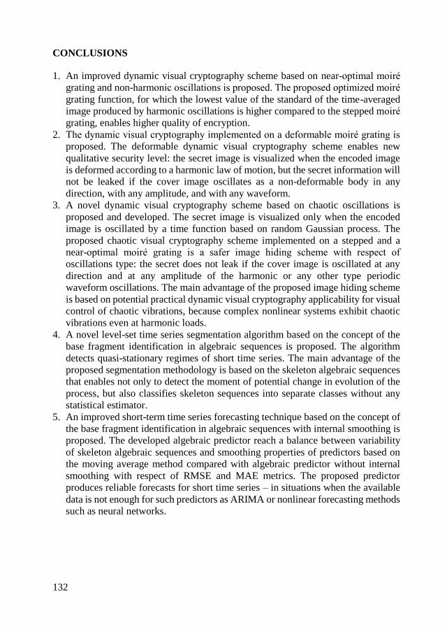
132
CONCLUSIONS
1. An improved dynamic visual cryptography scheme based on near-optimal moiré
grating and non-harmonic oscillations is proposed. The proposed optimized moiré
grating function, for which the lowest value of the standard of the time-averaged
image produced by harmonic oscillations is higher compared to the stepped moiré
grating, enables higher quality of encryption.
2. The dynamic visual cryptography implemented on a deformable moiré grating is
proposed. The deformable dynamic visual cryptography scheme enables new
qualitative security level: the secret image is visualized when the encoded image
is deformed according to a harmonic law of motion, but the secret information will
not be leaked if the cover image oscillates as a non-deformable body in any
direction, with any amplitude, and with any waveform.
3. A novel dynamic visual cryptography scheme based on chaotic oscillations is
proposed and developed. The secret image is visualized only when the encoded
image is oscillated by a time function based on random Gaussian process. The
proposed chaotic visual cryptography scheme implemented on a stepped and a
near-optimal moiré grating is a safer image hiding scheme with respect of
oscillations type: the secret does not leak if the cover image is oscillated at any
direction and at any amplitude of the harmonic or any other type periodic
waveform oscillations. The main advantage of the proposed image hiding scheme
is based on potential practical dynamic visual cryptography applicability for visual
control of chaotic vibrations, because complex nonlinear systems exhibit chaotic
vibrations even at harmonic loads.
4. A novel level-set time series segmentation algorithm based on the concept of the
base fragment identification in algebraic sequences is proposed. The algorithm
detects quasi-stationary regimes of short time series. The main advantage of the
proposed segmentation methodology is based on the skeleton algebraic sequences
that enables not only to detect the moment of potential change in evolution of the
process, but also classifies skeleton sequences into separate classes without any
statistical estimator.
5. An improved short-term time series forecasting technique based on the concept of
the base fragment identification in algebraic sequences with internal smoothing is
proposed. The developed algebraic predictor reach a balance between variability
of skeleton algebraic sequences and smoothing properties of predictors based on
the moving average method compared with algebraic predictor without internal
smoothing with respect of RMSE and MAE metrics. The proposed predictor
produces reliable forecasts for short time series – in situations when the available
data is not enough for such predictors as ARIMA or nonlinear forecasting methods
such as neural networks.
133
REFERENCES
1. Kabayashi, A. S. (1993). Handbook on Experimental Mechanics, 2nd ed., Bethel
SEM, 1074 p., IBSN: 978-0-471-18864-3.
2. Patorski K., Kujawinska M..(1995). Handbook of the Moiré Fringe Technique:
Amsterdam, Elsevier.
3. Post D., Han B., Ifju P. (1997) High Sensitivity Moiré: Experimental Analysis for
Mechanics and Materials, Springer, Verlag, Berlin.
4. Dai, F. L., & Wang, Z. Y. (1999). Geometric micron-moiré. [Article]. Optics and
Lasers in Engineering, 31(3), 191-198.
5. Desmedt, Y., van Le, T. (2000). Moiré cryptography. Seventh ACM Conference on
Computer and Communications Security, 116-124
6. Rayleigh., L. (1874) On the manufacture and theory of diffraction-gratings. Phil.
Mag.S.4, 47(310), 81-93, 193-205.
7. Weller, R., Shepherd, B. M. (1948) Displacement measurement by mechanical
interferometry. Proceedings of Society for Experimental Stress Analysis (SESA),
6(l), 35-38.
8. Kafri, O., Glatt, I. (1990) The Physics of Moiré Metrology. New York, Wiley.
9. Ragulskis, M., Maskeliunas, T., Ragulskis, T., Turla, V. (2005). Investigation of
dynamic displacements of lithographicpress rubber roller by time average
geometric moire. [Article]. Optics and Lasers in Engineering 43(4), 951-962.
10. Cloud, G. (2005). Optical methods in experimental mechanics - Part 18:
Geometric moire phenomena and simulations. [Article]. Experimental Techniques,
29(4), 15-18.
11. Howard, J. M. (2001). Optical design using computer graphics. [Article]. Applied
Optics, 40(19), 3225-3231.
12. Pokorski, K., & Patorski, K. (2010). Visualization of additive-type moire and
time-average fringe patterns using the continuous wavelet transform. [Article].
Applied Optics, 49(19), 3640-3651.
13. Aleksa, A., Saunoriene, L., & Ragulskis, M. (2008, Apr 24-25). Image encryption
based on stochastic geometric moire. Paper presented at the 14th International
Conference on Information and Software Technologies, Kaunas, LITHUANIA.
14. Kong, L. S., Cai, S., Li, Z. X., Jin, G., Huang, S. B., Xu, K., et al. (2011).
Interpretation of moire phenomenon in the image domain. [Article]. Optics
Express, 19(19), 18399-18409.
15. Yu, L., Wang, S. R., & Lin, G. Y. (2013). An image domain approach to the
interpretation of the visible moire phenomenon. [Article]. Journal of Optics, 15(7),
11.
16. Breque, C., Dupre, J. C., & Bremand, F. (2004). Calibration of a system of
projection moire for relief measuring: biomechanical applications. [Article].
Optics and Lasers in Engineering, 41(2), 241-260.
17. Cicinelli, V., Pappalettere, C., Sun, W. M., & Surface, L. (2000). Application of
134
geometric moire to the analysis of large deformation in three-dimensional models.
[Proceedings Paper]. Iutam Symposium on Advanced Optical Methods and
Applications in Solid Mechanics, 82, 611-618.
18. Ifju, P. G., & Han, B. (2010). Recent Applications of Moire Interferometry.
Experimental Mechanics, 50(8), 1129-1147.
19. McKelvie, J. (1998). Moire strain analysis: an introduction, review and critique,
including related techniques and future potential. [Article]. Journal of Strain
Analysis for Engineering Design, 33(2), 137-151.
20. Sciammarella, C. A., Lamberti, L., Boccaccio, A., & Sciammarella, F. M. (2011).
High Precision Contouring with Moire and Related Methods: A Review. [Review].
Strain, 47, 43-64.
21. Naor M., Shamir A., (1994). Visual cryptography, Lecture Notes in Computer
Science 950, 1–12.
22. Ateniese, G., Blundo, C., DeSantis, A., & Stinson, D. R. (1996). Visual
cryptography for general access structures. [Article]. Information and
Computation, 129(2), 86-106.
23. Zhou, Z., Arce, G. R., & Di Crescenzo, G. (2006). Halftone visual cryptography.
[Article]. Ieee Transactions on Image Processing, 15(8), 2441-2453.
24. Blundo, C., De Santis, A., & Naor, M. (2000). Visual cryptography for grey level
images. [Article]. Information Processing Letters, 75(6), 255-259.
25. Tharayil, J. J., Kumar, E. S. K., & Alex, N. S. (2012). Visual Cryptography Using
Hybrid Halftoning. [Proceedings Paper]. International Conference on Modelling
Optimization and Computing, 38, 2117-2123.
26. Monoth, T., & Anto, P. B. (2010). Contrast-Enhanced Visual Cryptography
Schemes Based on Additional Pixel Patterns. [Proceedings Paper]. 2010
International Conference on Cyberworlds (Cw 2010), 171-178.
27. Chen, Y. F., Chan, Y. K., Huang, C. C., Tsai, M. H., & Chu, Y. P. (2007). A
multiple-level visual secret-sharing scheme without image size expansion.
[Article]. Information Sciences, 177(21), 4696-4710.
28. Lee, C. C., Chen, H. H., Liu, H. T., Chen, G. W., & Tsai, C. S. (2014). A new
visual cryptography with multi-level encoding. [Article]. Journal of Visual
Languages and Computing, 25(3), 243-250.
29. Lee, K. H., & Chiu, P. L. (2013). Image Size Invariant Visual Cryptography for
General Access Structures Subject to Display Quality Constraints. [Article]. Ieee
Transactions on Image Processing, 22(10), 3830-3841.
30. Askari, N., Moloney, C., Heys, H. M., & Ieee. (2012). A Novel Visual Secret
Sharing Scheme without Image Size Expansion. [Proceedings Paper]. 2012 25th
Ieee Canadian Conference on Electrical & Computer Engineering (Ccece), 4.
31. Lee, K. H., & Chiu, P. L. (2011). A high contrast and capacity efficient visual
cryptography scheme for the encryption of multiple secret images. [Article].
135
Optics Communications, 284(12), 2730-2741.
32. Yang, C. N., & Laih, C. S. (2000). New colored visual secret sharing schemes.
[Article]. Designs Codes and Cryptography, 20(3), 325-336.
33. Hou, Y. C. (2003). Visual cryptography for color images. [Article]. Pattern
Recognition, 36(7), 1619-1629.
34. Shyu, S. H. (2006). Efficient visual secret sharing scheme for color images.
[Article]. Pattern Recognition, 39(5), 866-880.
35. Wang, D. S., Yi, F., & Li, X. B. (2011). Probabilistic visual secret sharing schemes
for grey-scale images and color images. [Article]. Information Sciences, 181(11),
2189-2208.
36. Shyu, S. J., Huang, S. Y., Lee, Y. K., Wang, R. Z., & Chen, K. (2007). Sharing
multiple secrets in visual cryptography. [Article]. Pattern Recognition, 40(12),
3633-3651.
37. Feng, J. B., Wu, H. C., Tsai, C. S., Chang, Y. F., & Chu, Y. P. (2008). Visual
secret sharing for multiple secrets. [Article]. Pattern Recognition, 41(12), 3572-
3581.
38. Yang, C. N., & Chung, T. H. (2010). A general multi-secret visual cryptography
scheme. [Article]. Optics Communications, 283(24), 4949-4962.
39. Lin, T. L., Horng, S. J., Lee, K. H., Chiu, P. L., Kao, T. W., Chen, Y. H., et al.
(2010). A novel visual secret sharing scheme for multiple secrets without pixel
expansion. [Article]. Expert Systems with Applications, 37(12), 7858-7869.
40. Hegde, C., Manu, S., Shenoy, P. D., Venugopal, K. R., & Patnaik, L. M. (2008).
Secure Authentication using Image Processing and Visual Cryptography for
Banking Applications. [Proceedings Paper]. Adcom: 2008 16th International
Conference on Advanced Computing and Communications, 65-72.
41. Chan, C. W., & Lin, C. H. (2008). A new credit card payment scheme using
mobile phones based on visual cryptography. [Proceedings Paper]. Intelligence
and Security Informatics, Proceedings, 5075, 467-476.
42. Rao, Y. V. S., Sukonkina, Y., Bhagwati, C., Singh, U. K., & Ieee. (2008, Nov 19-
21). Fingerprint based authentication application using visual cryptography
methods (Improved ID card). Paper presented at the IEEE Region 10 Conference
(TENCON 2008), Hyderabad, INDIA.
43. Ross, A., & Othman, A. (2011). Visual Cryptography for Biometric Privacy.
[Article]. Ieee Transactions on Information Forensics and Security, 6(1), 70-81.
44. Singh, T. R., Singh, K. M., & Roy, S. (2013). Video watermarking scheme based
on visual cryptography and scene change detection. [Article]. Aeu-International
Journal of Electronics and Communications, 67(8), 645-651.
45. Weir, J., Yan, W. Q., & Ieee. (2010). Resolution Variant Visual Cryptography for
Street View of Google Maps. [Proceedings Paper]. 2010 Ieee International
Symposium on Circuits and Systems, 1695-1698.
136
46. Hou, Y. C., & Quan, Z. Y. (2009). LEARNING WITH FUN An Application of
Visual Cryptography. [Proceedings Paper]. Csedu 2009: Proceedings of the First
International Conference on Computer Supported Education, Vol I, 456-459.
47. Amidror, I., Chosson, S., & Hersch, R. D. (2007, Sep 05-06). Moiré methods for
the protection of documents and products: A short survey - art. no. 012001. Paper
presented at the 11th International Congress of Stereology, St Etienne, FRANCE.
48. de Oliveira, G. N., Oliveira, M. E., & dos Santos, P. A. M. (2012, Aug 13-15).
Photorefractive moiré like pattern as optical numerical code generator. Paper
presented at the Conference on Interferometry XVI - Techniques and Analysis,
San Diego, CA.
49. de Oliveira, G. N., Oliveira, M. E., & dos Santos, P. A. M. (2013). Photorefractive
holographic moiré-like patterns for secure numerical code generation. [Article].
Optics Letters, 38(6), 1004-1006.
50. Zhao, X. M., & Xie, B. (2012). Halftone Image Processing Method of Security
Based on moiré Effect. [Proceedings Paper]. Packaging Science and Technology,
200, 712-718.
51. Y. Desmedt, Y., van Le, T. (2000) moiré Cryptography. 7th ACM Conf. Comput.
Commun. Secur., 116-124.
52. Munoz-Rodriguez, J. A., & Rodriguez-Vera, R. (2004). Image encryption based
on moiré pattern performed by computational algorithms. [Article]. Optics
Communications, 236(4-6), 295-301.
53. Murata, S., Morita, T., & Miyazaki, M. (2008). Hidden images on color
honeycomb moiré patterns. [Editorial Material]. Journal of Visualization, 11(2),
114-114.
54. Ragulskis, M., Aleksa, A., & Saunoriene, L. (2007). Improved algorithm for
image encryption based on stochastic geometric moiré and its application.
[Article]. Optics Communications, 273(2), 370-378.
55. Aleksa, A., Saunoriene, L., & Ragulskis, M. (2008, Apr 24-25). Image encryption
based on stochastic geometric moiré. Paper presented at the 14th International
Conference on Information and Software Technologies, Kaunas, LITHUANIA.
56. Fournel, T., & Ieee. (2012). Contrast-enhanced Moiré Cryptography.
[Proceedings Paper]. 2012 11th Euro-American Workshop on Information Optics
(Wio), 3.
57. Ragulskis, M., & Aleksa, A. (2009). Image hiding based on time-averaging moire.
[Article]. Optics Communications, 282(14), 2752-2759.
58. Ragulskis, M., Aleksa, A., & Ragulskiene, J. (2009). Image Hiding Based on
Circular Geometric Moire. [Proceedings Paper]. Recent Advances in Applied
Mathematics, 137-142.
59. Ragulskis, M., Aleksa, A., & Navickas, Z. (2009). Image hiding based on time-
137
averaged fringes produced by non-harmonic oscillations. [Article]. Journal of
Optics a-Pure and Applied Optics, 11(12), 11.
60. Astrom, K. J., (1969). On the choice of sampling rates in parametric identification
of time series. Information Sciences 1 (3), 273–278.
61. Yi, B., Faloutsos, C., (2000). Fast time sequence indexing for arbitrary Lp norms.
In: Proceedings of the 26th International Conference on Very Large Data Bases,
pp. 385–394.
62. Guo, C. H., Li, H. L., & Pan, D. H. (2010). An Improved Piecewise Aggregate
Approximation Based on Statistical Features for Time Series Mining. [Proceedings
Paper]. Knowledge Science, Engineering and Management, 6291, 234-244.
63. Keogh, E., Chu, S., Hart, D., Pazzani, M., (2001). An online algorithm for
segmenting time series. In: Proceedings of the 2001 IEEE International
Conference on Data Mining, pp. 289–296.
64. Shatkay, H., & Zdonik, S. B. (1996, Feb 26-Mar 01). Approximate queries and
representations for large data sequences. Paper presented at the 12th International
Conference on Data Engineering, New Orleans, La.
65. Li, C., Yu, P., Castelli, V. (1998). MALM: A framework for mining sequence
database at multiple abstraction levels. Proceedings of the 7th International
Conference on Information and Knowledge Management, 267-272.
66. Keogh, E.J.; Pazzani, M.J. (1998). An enhanced representation of time series
which allows fast and accurate classification, clustering and relevance feedback.
Proceedings of the Fourth International Conference on Knowledge Discovery and
Data Mining: New York, NY, USA, 239-243.
67. Lemire, D. (2007). A Better Alternative to Piecewise Linear Time Series
Segmentation. [Proceedings Paper]. Proceedings of the Seventh Siam International
Conference on Data Mining, 545-550.
68. Terzi, E., & Tsaparas, P. (2006, Apr 20-22). Efficient algorithms for sequence
segmentation. Paper presented at the 6th SIAM International Conference on Data
Mining, Bethesda, MD.
69. Lopatka, M., Laplanche, C., Adam, O., Motsch, J. F., Zarzycki, J., & Ieee. (2005).
Non-stationary time-series segmentation based on the Schur prediction error
analysis. [Proceedings Paper]. 2005 IEEE/SP 13th Workshop on Statistical Signal
Processing (SSP), Vols 1 and 2, 224-228.
70. Azami, F., Sanei, S., Mohammadi, K., & Hassanpour, H. (2013). A hybrid
evolutionary approach to segmentation of non-stationary signals. [Article]. Digital
Signal Processing, 23(4), 1103-1114.
71. Jiao, B., Krishnan, S., & Kabbani, A. (2010). FPGA implementation of adaptive
segmentation for non-stationary biomedical signals. [Article]. Iet Circuits Devices
& Systems, 4(3), 239-250.
72. Anisheh, S. M., & Hassanpour, H. (2011). Designing an adaptive approach for
138
segmenting non-stationary signals. [Article]. International Journal of Electronics,
98(8), 1091-1102.
73. Davis, R. A., Lee, T. C. M., & Rodriguez-Yam, G. A. (2006). Structural break
estimation for nonstationary time series models. [Article]. Journal of the American
Statistical Association, 101(473), 223-239.
74. Cheng, X. G., Li, B., & Chen, Q. M. (2011). On-Line Structural Breaks Estimation
for Non-stationary Time Series Models. [Article]. China Communications, 8(7),
95-104.
75. Sato, A. H., & Ieee. (2013, Jul 22-26). Recursive segmentation procedure based
on the Akaike information criterion test. Paper presented at the IEEE 37th Annual
Computer Software and Applications Conference (COMPSAC), Kyoto, JAPAN.
76. Toth, B., Lillo, F., & Farmer, J. D. (2010). Segmentation algorithm for non-
stationary compound Poisson processes. [Article]. European Physical Journal B,
78(2), 235-243.
77. Camargo, S., Queiros, S. M. D., & Anteneodo, C. (2011). Nonparametric
segmentation of nonstationary time series. [Article]. Physical Review E, 84(4), 7
78. Song, L., & Bondon, P. (2013). Structural changes estimation for strongly
dependent processes. [Article]. Journal of Statistical Computation and Simulation,
83(10), 1783-1806.
79. Bernaola-Galvan, P., Oliver, J. L., Hackenberg, M., Coronado, A. V., Ivanov, P.
C., & Carpena, P. (2012). Segmentation of time series with long-range fractal
correlations. [Article]. European Physical Journal B, 85(6), 12.
80. Karaliene, D., Navickas, Z., & Vainoras, A. (2012). Segmentation Algorithm for
Algebraic Progressions. [Proceedings Paper]. Information and Software
Technologies, 319, 149-161.
81. Vo, V., Luo, J. W., & Vo, B. (2013). Dimensionality Reduction by Turning Points
for Stream Time Series Prediction. [Proceedings Paper]. Advanced Methods for
Computational Collective Intelligence, 457, 167-176.
82. Fuchs, E., Gruber, T., Pree, H., & Sick, B. (2010). Temporal data mining using
shape space representations of time series. [Article]. Neurocomputing, 74(1-3),
379-393.
83. Xu, K. K., Jiang, Y. X., Tang, M. J., Yuan, C. G., & Tang, C. J. (2013). PRESEE:
An MDL/MML Algorithm to Time-Series Stream Segmenting. [Article]. Scientific
World Journal, 11.
84. Li, G. L., Cai, Z. H., Kang, X. J., Wu, Z. D., & Wang, Y. Z. (2014). ESPSA: A
prediction-based algorithm for streaming time series segmentation. [Article].
Expert Systems with Applications, 41(14), 6098-6105.
85. Haiminen, N., & Mannila, H. (2010). Evaluation of BIC and Cross Validation for
model selection on sequence segmentations. [Article]. International Journal of
139
Data Mining and Bioinformatics, 4(6), 675-700.
86. Nam, C. F. H., Aston, J. A. D., & Johansen, A. M. (2012). Quantifying the
uncertainty in change points. [Article]. Journal of Time Series Analysis, 33(5),
807-823.
87. Rienzner, M., & Gandolfi, C. (2011). A composite statistical method for the
detection of multiple undocumented abrupt changes in the mean value within a
time series. [Article]. International Journal of Climatology, 31(5), 742-755.
88. Lai, T. L., & Xing, H. P. (2013). STOCHASTIC CHANGE-POINT ARX-
GARCH MODELS AND THEIR APPLICATIONS TO ECONOMETRIC TIME
SERIES. [Article]. Statistica Sinica, 23(4), 1573-1594.
89. Sismeiro, C., Mizik, N., & Bucklin, R. E. (2012). Modeling coexisting business
scenarios with time-series panel data: A dynamics-based segmentation approach.
[Article]. International Journal of Research in Marketing, 29(2), 134-147.
90. Vaglica, G., Lillo, F., & Mantegna, R. N. (2010). Statistical identification with
hidden Markov models of large order splitting strategies in an equity market.
[Article]. New Journal of Physics, 12, 24.
91. Wong, J. C., Lian, H., & Cheong, S. A. (2009). Detecting macroeconomic phases
in the Dow Jones Industrial Average time series. [Article]. Physica a-Statistical
Mechanics and Its Applications, 388(21), 4635-4645.
92. Cheong, S. A., Fornia, R. P., Lee, G. H. T., Kok, J. L., Yim, W. S., Xu, D. Y., et
al. (2012). The Japanese Economy in Crises: A Time Series Segmentation Study.
[Article]. Economics-the Open Access Open-Assessment E-Journal, 6, 82.
93. Hamilton, J. D. (1989). A NEW APPROACH TO THE ECONOMIC-ANALYSIS
OF NONSTATIONARY TIME-SERIES AND THE BUSINESS-CYCLE.
[Article]. Econometrica, 57(2), 357-384.
94. Fushing, H., Chen, S. C., & Lee, H. J. (2010). Statistical Computations on
Biological Rhythms I: Dissecting Variable Cycles and Computing Signature
Phases in Activity-Event Time Series. [Article]. Journal of Computational and
Graphical Statistics, 19(1), 221-239.
95. Bru, N., Biritxinaga, E., & D'Amico, F. (2011). Detection of significant changes
in short time series: applications to the analysis of annual routines in behavioural
ecology and to the analysis of breaks in abundance. [Proceedings Paper]. 19th
International Congress on Modelling and Simulation (Modsim2011), 2211-2218.
96. Graef, A., Flamm, C., Pirker, S., Deistler, M., Baumgartner, C., & Ieee. (2012,
Aug 28-Sep 01). A physiologically motivated ECoG segmentation method for
epileptic seizure onset zone detection. Paper presented at the 34th Annual
International Conference of the IEEE Engineering-in-Medicine-and-Biology-
Society (EMBS), San Diego, CA.
97. Latchoumane, C. F. V., & Jeong, J. (2011). Quantification of Brain Macrostates

140
Using Dynamical Nonstationarity of Physiological Time Series. [Article]. Ieee
Transactions on Biomedical Engineering, 58(4), 1084-1093.
98. Darkhovsky, B., Piryatinska, A., & Ieee. (2012). A new complexity-based
algorithmic procedures for electroencephalogram (EEG) segmentation.
[Proceedings Paper]. 2012 Ieee Signal Processing in Medicine and Biology
Symposium (Spmb), 5.
99. Vakorin, V. A., McIntosh, A. R., Misic, B., Krakovska, O., Poulsen, C., Martinu,
K., et al. (2013). Exploring Age-Related Changes in Dynamical Non-Stationarity
in Electroencephalographic Signals during Early Adolescence. [Article]. Plos One,
8(3), 10.
100. Mico, P., Mora, M., Cuesta-Frau, D., & Aboy, M. (2010). Automatic
segmentation of long-term ECG signals corrupted with broadband noise based on
sample entropy. [Article]. Computer Methods and Programs in Biomedicine,
98(2), 118-129.
101. De Roover, K., Timmerman, M. E., Van Diest, I., Onghena, P., & Ceulemans,
E. (2014). Switching Principal Component Analysis for Modeling Means and
Covariance Changes Over Time. [Article]. Psychological Methods, 19(1), 113-32.
102. Brown, R. G. (1963). Smoothing, forecasting and prediction of discrete time
series. Englewood Cliffs, NJ: Prentice-Hall.
103. Gardner Jr., E. S. (1985). Exponential smoothing: the state of art. Journal of
Forecasting, 4, 1-38.
104. Gelper, S., Fried, R., & Croux, C. (2010). Robust Forecasting with Exponential
and Holt-Winters Smoothing. [Article]. Journal of Forecasting, 29(3), 285-300.
105. Hyndman, R.J. Moving Averages, 2008 [interactive] [2014-03-14]. Website:
http://robjhyndman.com/papers/movingaverage.pdf.
106. Box, G. E. P., Jenkins, G. M., & Reinsel G. C. (1994). Time series analysis:
forecasting and control (3rd. ed.). Englewood Cliffs, NJ: Prentice-Hall.
107. Lee, Y. S., & Tong, L. I. (2011). Forecasting time series using a methodology
based on autoregressive integrated moving average and genetic programming.
[Article]. Knowledge-Based Systems, 24(1), 66-72.
108. Contreras, J., Espinola, R., Nogales, F. J., & Conejo, A. J. (2003). ARIMA
models to predict next-day electricity prices. [Article]. Ieee Transactions on Power
Systems, 18(3), 1014-1020.
109. Conejo, A. J., Plazas, M. A., Espinola, R., & Molina, A. B. (2005). Day-ahead
electricity price forecasting using the wavelet transform and ARIMA models.
[Article]. Ieee Transactions on Power Systems, 20(2), 1035-1042.
110. Zhang, G. Q., Patuwo, B. E., & Hu, M. Y. (1998). Forecasting with artificial
neural networks: The state of the art. [Review]. International Journal of
Forecasting, 14(1), 35-62.
141
111. Adya, M., & Collopy, F. (1998). How effective are neural networks at
forecasting and prediction? A review and evaluation. [Article]. Journal of
Forecasting, 17(5-6), 481-495.
112. Adamowski, J., & Karapataki, C. (2010). Comparison of Multivariate
Regression and Artificial Neural Networks for Peak Urban Water-Demand
Forecasting: Evaluation of Different ANN Learning Algorithms. [Article]. Journal
of Hydrologic Engineering, 15(10), 729-743.
113. Tseng, F. M., Yu, H. C., & Tzeng, G. H. (2002). Combining neural network
model with seasonal time series ARIMA model. [Article]. Technological
Forecasting and Social Change, 69(1), 71-87.
114. Kourentzes, N., Barrow, D. K., & Crone, S. F. (2014). Neural network ensemble
operators for time series forecasting. [Article]. Expert Systems with Applications,
41(9), 4235-4244.
115. Diebold, F. (2007). Elements of Forecasting. (Fourth edition) South-Western
College Publishing Cincinnati, Ohio.
116. Pagacz, P. (2012). On Wold-type decomposition. [Article]. Linear Algebra and
Its Applications, 436(9), 3065-3071.
117. Dickey, D. A.; Fuller, W. A. (1979). Distribution of the Estimators for
Autoregressive Time Series with a Unit Root. Journal of the American Statistical
Association 74 (366): 427–431.
118. Elliott, G., Rothenberg, T. J., & Stock, J. H. (1996). Efficient tests for an
autoregressive unit root. [Article]. Econometrica, 64(4), 813-836.
119. Bisgaard, S., Kulahci, M. (2011). Time series analysis and forecasting by
example. Hoboken [N.J.]: Wiley.
120. Hyndman, R. J. & Kostenko, A. V. (2007) Minimum sample size requirements
for seasonal forecasting models, Foresight: the International Journal of Applied
Forecasting 6, 12–15.
121. Akaike, H. (1974). A new look at the statistical model identification, IEEE
Transactions on Automatic Control 19 (6): 716–723.
122. Schwarz, G. (1978). Estimating the dimension of a model. Annals of Statistics
6(2), 461-464.
123. Box, G. E. P. and Pierce, D. A. (1970). Distribution of Residual Autocorrelations
in Autoregressive-Integrated Moving Average Time Series Models, Journal of the
American Statistical Association, 65: 1509–1526.
124. Jarque, Carlos M.; Bera, Anil K. (1980). "Efficient tests for normality,
homoscedasticity and serial independence of regression residuals". Economics
Letters 6 (3): 255–259.
125. Kurakin, V.L., Kuzmin, A.S., Michalev, A.V., Nechaev, A.A. (1995). Linear
recurring sequences over rings and modules, Journal of Mathematical Sciences
142
76(6), 2793–2915.
126. Navickas, Z., Bikulciene, L. (2006). Expressions of solutions of ordinary
differential equations by standard functions, Mathematical Modelling and Analysis
11, 399-412.
127. Makridakis, S. G., Wheelwright, S.C., Hyndman, R.J. (1998). Forecasting:
methods and applications (3rd ed.). New York [etc.] : John Wiley.
128. Ardalani-Farsa, M., & Zolfaghari, S. (2010). Chaotic time series prediction with
residual analysis method using hybrid Elman-NARX neural networks. [Article].
Neurocomputing, 73(13-15), 2540-2553.
129. Hill, T., Oconnor, M., & Remus, W. (1996). Neural network models for time
series forecasts. [Article]. Management Science, 42(7), 1082-1092.
130. Kaastra, I., & Boyd, M. (1996). Designing a neural network for forecasting
financial and economic time series. [Article]. Neurocomputing, 10(3), 215-236.
131. Hadavandi, E., Shavandi, H., & Ghanbari, A. (2010). Integration of genetic fuzzy
systems and artificial neural networks for stock price forecasting. [Article].
Knowledge-Based Systems, 23(8), 800-808.
132. Cai, Y. A., Wang, J. Z., Tang, Y., & Yang, Y. C. (2011). An efficient approach
for electric load forecasting using distributed ART (adaptive resonance theory) &
HS-ARTMAP (Hyper-spherical ARTMAP network) neural network. [Article].
Energy, 36(2), 1340-1350.
133. Chang, F. J., Chen, P. A., Lu, Y. R., Huang, E., & Chang, K. Y. (2014). Real-
time multi-step-ahead water level forecasting by recurrent neural networks for
urban flood control. [Article]. Journal of Hydrology, 517, 836-846.
134. Chen, A., Leung, M. T., & Hazem, D. (2003). Application of neural networks to
an emerging financial market: Forecasting and trading the Taiwan Stock Index.
Computers and Operations Research, 30, 901–923.
135. Zhang, G. P., & Qi, G. M. (2005). Neural network forecasting for seasonal and
trend time series. European Journal of Operational Research, 160, 501-514.
136. Khashei, M., & Bijari, M. (2010). An artificial neural network (p, d, q) model
for timeseries forecasting. [Article]. Expert Systems with Applications, 37(1), 479-
489.
137. Khashei, M., & Bijari, M. (2011). A novel hybridization of artificial neural
networks and ARIMA models for time series forecasting. [Article]. Applied Soft
Computing, 11(2), 2664-2675.
138. Zurada, J. M., Kang, M. J., & Ieee. (1991). NUMERICAL MODELING OF
CONTINUOUS-TIME FULLY COUPLED NEURAL NETWORKS.
[Proceedings Paper]. 1991 Ieee International Joint Conference on Neural
Networks, Vols 1-3, 1924-1929.
139. De Gooijer, J. G., & Hyndman, R. J. (2006). 25 years of time series forecasting.
143
[Review]. International Journal of Forecasting, 22(3), 443-473.
140. Clements, M. P. (2003). Some possible directions for future research. [Editorial
Material]. International Journal of Forecasting, 19(1), 1-3.
141. Brownston, , D. (1996). Using percentage accuracy to measure neural network
predictions in Stock Market movements. [Article]. Neurocomputing, (10)3, 237-
250.
142. Hibon, M., & Evgeniou, T. (2005). To combine or not to combine: selecting
among forecasts and their combinations. [Article]. International Journal of
Forecasting, 21(1), 15-24.
143. Zhang, G. P. (2003). Time series forecasting using a hybrid ARIMA and neural
network model. [Article]. Neurocomputing, 50, 159-175.
144. Khashei, M., & Bijari, M. (2012). A new class of hybrid models for time series
forecasting. Expert Systems with Applications, 39(4), 4344-4357.
145. Wang, J. J., Wang, J. Z., Zhang, Z. G., & Guo, S. P. (2012). Stock index
forecasting based on a hybrid model. [Article]. Omega-International Journal of
Management Science, 40(6), 758-766.
146. Chan, K. Y., Dillon, T. S., Singh, J., & Chang, E. (2012). Neural-Network-Based
Models for Short-Term Traffic Flow Forecasting Using a Hybrid Exponential
Smoothing and Levenberg-Marquardt Algorithm. [Article]. Ieee Transactions on
Intelligent Transportation Systems, 13(2), 644-654.
147. Maia, A. L. S., & de Carvalho, F. D. T. (2011). Holt's exponential smoothing and
neural network models for forecasting interval-valued time series. [Article].
International Journal of Forecasting, 27(3), 740-759.
148. Babu, C. N., & Reddy, B. E. (2014). A moving-average filter based hybrid
ARIMA-ANN model for forecasting time series data. [Article]. Applied Soft
Computing, 23, 27-38.
149. Christiaanse, W.R., (1971). Short term load forecasting using general
exponential smoothing, IEEE Trans. Power Apparatus Syst. 90, 900–911.
150. Taylor, J. W. (2012). Short-Term Load Forecasting With Exponentially
Weighted Methods. [Article]. Ieee Transactions on Power Systems, 27(1), 458-
464.
151. Hippert, H. S., Pedreira, C. E., & Souza, R. C. (2001). Neural networks for short-
term load forecasting: A review and evaluation. [Review]. Ieee Transactions on
Power Systems, 16(1), 44-55.
152. Fan, S., & Hyndman, R. J. (2012). Short-Term Load Forecasting Based on a
Semi-Parametric Additive Model. [Article]. Ieee Transactions on Power Systems,
27(1), 134-141.
153. Chen, Y., Luh, P. B., Guan, C., Zhao, Y., Michel, L. D., Coolbeth, M. A., et al.
(2010). Short-Term Load Forecasting: Similar Day-Based Wavelet Neural
144
Networks. [Article]. Ieee Transactions on Power Systems, 25(1), 322-330.
154. Kani, S. A. P., & Ardehali, M. M. (2011). Very short-term wind speed prediction:
A new artificial neural network-Markov chain model. [Article]. Energy
Conversion and Management, 52(1), 738-745.
155. Dong, Y., Wang, J. Z., Jiang, H., & Wu, J. (2011). Short-term electricity price
forecast based on the improved hybrid model. [Article]. Energy Conversion and
Management, 52(8-9), 2987-2995.
156. Catalao, J. P. S., Pousinho, H. M. I., & Mendes, V. M. F. (2011). Hybrid
Wavelet-PSO-ANFIS Approach for Short-Term Electricity Prices Forecasting.
[Article]. Ieee Transactions on Power Systems, 26(1), 137-144.
157. Lee, C.M., Ko, C.N. (2009) Time series prediction using RBF neural networks
witha nonlinear time-varying evolution PSO algorithm, Neurocomputing 73(1–3),
449–460.
158. Bashir, Z.A., El-Hawary, M.E. (2009). Applying wavelets to short-term load
forecasting using PSO-based neural networks, IEEE Trans. Power Syst. 24(1),
20–27.
159. Casolari, S., Colajanni, M. (2009) Short-term prediction models for server
management in Internet-based contexts, Decis. Support Syst. 48(1), 212–223.
160. Weigend, A. S., Gershenfeld, N. A., & Ieee. (1993). RESULTS OF THE TIME-
SERIES PREDICTION COMPETITION AT THE SANTA-FE INSTITUTE.
[Proceedings Paper]. 1993 Ieee International Conference on Neural Networks,
Vols 1-3, 1786-1793.
161. Diebold, F. X., & Mariano, R. S. (1995). COMPARING PREDICTIVE
ACCURACY. [Article]. Journal of Business & Economic Statistics, 13(3), 253-
263.
162. Hyndman, R. J., & Koehler, A. B. (2006). Another look at measures of forecast
accuracy. [Article]. International Journal of Forecasting, 22(4), 679-688.
163. Li, S., Kang, L. Y., & Zhao, X. M. (2014). A Survey on Evolutionary Algorithm
Based Hybrid Intelligence in Bioinformatics. Biomed Research International, 8.
164. Schimit, P. H. T. (2014). On exploring the genetic algorithm for modeling the
evolution of cooperation in a population. Communications in Nonlinear Science
and Numerical Simulation, 19(8), 2801-2810.
165. Sinha, A., Malo, P., Frantsev, A., & Deb, K. (2014). Finding optimal strategies
in a multi-period multi-leader-follower Stackelberg game using an evolutionary
algorithm. Computers & Operations Research, 41, 374-385.
166. Chen, C. W., & Chen, P. C. (2010). GA-BASED ADAPTIVE NEURAL
NETWORK CONTROLLERS FOR NONLINEAR SYSTEMS. [Article].
International Journal of Innovative Computing Information and Control, 6(4),
1793-1803.
167. Belciug, S., & Gorunescu, F. (2013). A hybrid neural network/genetic algorithm
145
applied to breast cancer detection and recurrence. [Article]. Expert Systems, 30(3),
243-254.
168. Glezakos, T. J., Tsiligiridis, T. A., & Yialouris, C. P. (2014). Piecewise
evolutionary segmentation for feature extraction in time series models. [Article].
Neural Computing & Applications, 24(2), 243-257.
169. Sheikhan, M., & Mohammadi, N. (2012). Neural-based electricity load
forecasting using hybrid of GA and ACO for feature selection. [Article]. Neural
Computing & Applications, 21(8), 1961-1970.
170. Wu, J., Chan, C. K., Zhang, Y., Xiong, B. Y., & Zhang, Q. H. (2014). Prediction
of solar radiation with genetic approach combing multi-model framework.
[Article]. Renewable Energy, 66, 132-139.
171. Khodaei, M., & Faez, K. (2010). Image Hiding by Using Genetic Algorithm and
LSB Substitution. [Proceedings Paper]. Image and Signal Processing,
Proceedings, 6134, 404-411.
172. Prema, G., Natarajan, S., & Ieee. (2013). Steganography using Genetic
Algorithm along with Visual Cryptography for Wireless Network Application.
[Proceedings Paper]. 2013 International Conference on Information
Communication and Embedded Systems (Icices), 727-730.
173. Goldberg, D. E. (1989) Genetic Algorithms in Search, Optimization and Machine
Learning (1st ed.). Addison-Wesley Longman Publishing Co., Inc., Boston, MA,
USA.
174. Sharma A., Metha A. (2013). Review Paper of Various Selection Methods in
Genetic Algorithm. International Journal of Advanced Research in Computer
Science and Software Engineering, 3(7), 1476-1479.
175. Abuiziah I., Shakarneh N. (2013). A Review of Genetic Algorithm Optimization:
Operations and Applications to Water Pipeline Systems. World Academy of
Science, Engineering and Technology International Journal of Physical, Nuclear
Science and Engineering 7(12), 335-341.
176. Safe, M., Carballido, J., Ponzoni, I., & Brignole, N. (2004). On stopping criteria
for genetic algorithms. [Article; Proceedings Paper]. Advances in Artificial
Intelligence - Sbia 2004, 3171, 405-413.
177. Kennedy, J., Eberhart, R., & Ieee. (1995). Particle swarm optimization.
[Proceedings Paper]. 1995 Ieee International Conference on Neural Networks
Proceedings, Vols 1-6, 1942-1948.
178. Wang, J. Z., Zhu, S. L., Zhang, W. Y., & Lu, H. Y. (2010). Combined modeling
for electric load forecasting with adaptive particle swarm optimization. [Article].
Energy, 35(4), 1671-1678.
179. Bakkiyaraj, R. A., & Kumarappan, N. (2013). Optimal reliability planning for a
composite electric power system based on Monte Carlo simulation using particle
swarm optimization. [Article]. International Journal of Electrical Power &
Energy Systems, 47, 109-116.
180. AlRashidi, M. R., & El-Hawary, M. E. (2009). A Survey of Particle Swarm
Optimization Applications in Electric Power Systems. [Article]. Ieee Transactions
146
on Evolutionary Computation, 13(4), 913-918.
181. Kuo, R. J., Hong, S. Y., & Huang, Y. C. (2010). Integration of particle swarm
optimization-based fuzzy neural network and artificial neural network for supplier
selection. [Article]. Applied Mathematical Modelling, 34(12), 3976-3990.
182. Su, T. J., Cheng, J. C., Huang, M. Y., Lin, T. H., & Chen, C. W. (2011).
Applications of Cellular Neural Networks to Noise Cancelation in Gray Images
Based on Adaptive Particle-swarm Optimization. [Article]. Circuits Systems and
Signal Processing, 30(6), 1131-1148.
183. Quan, H., Srinivasan, D., & Khosravi, A. (2014). Particle swarm optimization
for construction of neural network-based prediction intervals. [Article].
Neurocomputing, 127, 172-180.
184. Chan, K. Y., Dillon, T. S., & Chang, E. (2013). An Intelligent Particle Swarm
Optimization for Short-Term Traffic Flow Forecasting Using on-Road Sensor
Systems. [Article]. Ieee Transactions on Industrial Electronics, 60(10), 4714-
4725.
185. Singh, P., & Borah, B. (2014). Forecasting stock index price based on M-factors
fuzzy time series and particle swarm optimization. [Article]. International Journal
of Approximate Reasoning, 55(3), 812-833.
186. Eberhart, R. C., Shi, Y., & Ieee. (2000). Comparing inertia weights and
constriction factors in particle swarm optimization. [Proceedings Paper].
Proceedings of the 2000 Congress on Evolutionary Computation, Vols 1 and 2,
84-88.
187. Clerc, M., & Kennedy, J. (2002). The particle swarm - Explosion, stability, and
convergence in a multidimensional complex space. [Article]. Ieee Transactions on
Evolutionary Computation, 6(1), 58-73.
188. Ozcan, E., Mohan, C.K. (1998) Analysis of a simple particle swarm
optimization system. [Article]. Intelligent Engineering Systems through Artificial
Neural Networks, 253–258.
189. Trelea, I. C. (2003). The particle swarm optimization algorithm: convergence
analysis and parameter selection. [Article]. Information Processing Letters, 85(6),
317-325.
190. van den Bergh, F., Engelbrecht A.P. (2006) A study of particle swarm
optimization particle trajectories. [Article]. Information Sciences, 176(8), 937-971
191. Jiang, M., Luo, Y. P., & Yang, S. Y. (2007). Stochastic convergence analysis
and parameter selection of the standard particle swarm optimization algorithm.
[Article]. Information Processing Letters, 102(1), 8-16.
192. Jordehi, A. R., & Jasni, J. (2013). Parameter selection in particle swarm
optimisation: a survey. [Article]. Journal of Experimental & Theoretical Artificial
Intelligence, 25(4), 527-542.
193. Sandeep, K., Vedpal, S., Gurbaj S., Alok, J. (2013). The Proposed Algorithm:
Image Security Technique in Visual Cryptography. Open Journal of Computer
Sciences, 1(1), 1-6.
194. Swadas, P. B., Patel, S., Darji, D. (2014). A comparatively study on visual
cryptography. International Journal of Research in Engineering and Technology,
147
3(1), 182-185.
195. Morampudi, N. K., Datrika, S. R., Sravanthi D. (2011). A novel approach for
cheating prevention through visual cryptographic analysis. [Article]. International
Journal of Computer Science & Engineering Survey (IJCSES), 4(2), 123-131.
196. Akshatha, M. M., Lokesh, B., Nuthan, A. C. (2014). Visual Cryptographic
Technique for Enhancing the Security of Image Transaction. [Article].
International Journal of Innovative Research in Computer and Communication
Engineering, 2(5), 4413-4418.
197. Horng, G., Chen, T., & Tsai, D. (2006). Cheating in visual cryptography.
[Article]. Designs Codes and Cryptography, 38(2), 219-236.
198. Chen, Y. C., Horng, G., & Tsai, D. S. (2012). Comment on "Cheating Prevention
in Visual Cryptography". [Editorial Material]. Ieee Transactions on Image
Processing, 21(7), 3319-3323.
199. Huang, Y. J., Chang, J. D., & Ieee. (2013). Non-expanded Visual Cryptography
Scheme with Authentication. [Proceedings Paper]. Ieee International Symposium
on Next-Generation Electronics 2013 (Isne 2013), 4.
200. De Prisco, R., & De Santis, A. (2010). Cheating Immune Threshold Visual Secret
Sharing. [Article]. Computer Journal, 53(9), 1485-1496.
201. Chen, Y. C., Tsai, D. S., & Horng, G. (2012). A new authentication based
cheating prevention scheme in Naor-Shamir's visual cryptography. [Article].
Journal of Visual Communication and Image Representation, 23(8), 1225-1233.
202. Liu, F., Wu, C., & Lin, X. (2011). Cheating immune visual cryptography scheme.
[Article]. Iet Information Security, 5(1), 51-59. 203. Verma, J., Khemchandani, V. (2012). A Visual Cryptographic Technique to
Secure Image Shares. International Journal of Engineering Research and
Applications (IJERA) 2(1), 1121-1125.
204. Benyoussef, M., Mabtoul, S., el Marraki, M., Aboutajdine, D. (2014). Robust
image watermarking scheme using visual cryptography in dual-tree complex
wavelet domain, Journal of Theoretical and Applied Information Technology,
60(2), 372-379.
205. Aleksa, A. (2011). [Dissertation]. Dinaminė vizualinė kriptografija – metodas ir
algoritminė realizacija, p 101.
206. Ramya, J., Parvathavarthini, B. (2014). An Extensive Review on Visual
Cryptography Schemes. International Conference on Control, Instrumentation,
Communication and Computational Technologies (ICCICCT), 223-228.
207. Pandey, D., Kumar, A., Singh, Y. (2013). Feature and future of visual
cryptography based schemes. Quality, Reliability, Security and Robustness in
Heterogeneous Networks. Lecture Notes of the Institute for Computer Sciences,
Social Informatics and Telecommunications Engineering 115, 816-830.
208. Weir, J., WeiQi Y. (2010). A Comprehensive Study of Visual Cryptography.
Transactions on DHMS V, LNCS 6010, 70–105.
209. Revenkar, P.S., Anjum A., Gandhare, W .Z. (2010). Survey of Visual
Cryptography Schemes. [Article]. International Journal of Security and Its
Applications, 4(2), 56.
148
210. Soradge N., Thakare K. S. (2014). A Review on Various Visual Cryptography
Schemes. International Journal of Computer Science and Business Informatics,
12(1), 45-54.
211. Jung-San Lee, T. Hoang Ngan Le, (2009). Hybrid (2, N) Visual Secret Sharing
Scheme For Color Images, 978-1- 4244-4568-4/09, IEEE.
212. Jaafar, A.M., Samsudin, A. (2010). A new public-key encryption scheme based
on non-expansion visual cryptography and Boolean operation, IJCSI International
Journal of Computer Science Issues 4(2), 1-10.
213. Hofmeister, T., Krause, M., & Simon, H. U. (2000). Contrast-optimal k out of n
secret sharing schemes in visual cryptography. [Article; Proceedings Paper].
Theoretical Computer Science, 240(2), 471-485.
214. Ito, R., Kuwakado, H., & Tanaka, H. (1999). Image size invariant visual
cryptography. [Article]. Ieice Transactions on Fundamentals of Electronics
Communications and Computer Sciences, E82A(10), 2172-2177.
215. Tuyls, P., Hollmann, H.D.L., van Lint, J.H., Tolhuizen, L.M.G.M. (2005). XOR-
based visual cryptography schemes. Designs, Codes and Cryptography 37(1),
169–186.
216. Petrauskiene, V., Aleksa, A., Fedaravicius, A., & Ragulskis, M. (2012). Dynamic
visual cryptography for optical control of vibration generation equipment. Optics
and Lasers in Engineering, 50(6), 869-876.
217. Ragulskis, M., Aleksa, A., & Maskeliunas, R. (2009). Contrast enhancement of
time-averaged fringes based on moving average mapping functions. [Article].
Optics and Lasers in Engineering, 47(7-8), 768-773.
218. Ragulskis, M., Saunoriene, L., & Maskeliunas, R. (2009). THE STRUCTURE
OF MOIRE GRATING LINES AND ITS INFLUENCE TO TIME-AVERAGED
FRINGES. [Article]. Experimental Techniques, 33(2), 60-64.
219. C.C. Wu, L.H. Chen, (1998). A study on visual cryptography. Master Thesis,
Institute of Computer and Information Science, National Chaio Tung University,
Taiwan, R.O.C.
220. Lee, K. H., & Chiu, P. L. (2011). A high contrast and capacity efficient visual
cryptography scheme for the encryption of multiple secret images. [Article].
Optics Communications, 284(12), 2730-2741.
221. Hilborn R. Chaos and Nonlinear Dinamics: an Introduction for Scientists and
Engineers. Oxford: Oxford University Press; 1994.
222. Sakyte, E., Palivonaite, R., Aleksa, A., & Ragulskis, M. (2011). Image hiding
based on near-optimal moire gratings. [Article]. Optics Communications, 284(16-
17), 3954-3964.
223. Whitley, D. (1994). A GENETIC ALGORITHM TUTORIAL. [Article].
Statistics and Computing, 4(2), 65-85.
149
224. Ragulskis, M., & Navickas, Z. (2007). Hash function construction based on time
average moire. [Article]. Discrete and Continuous Dynamical Systems-Series B,
8(4), 1007-1020.
225. Ragulskis, M., Sanjuan, M. A. F., & Saunoriene, L. (2007). Applicability of
time-average moire techniques for chaotic oscillations. [Article]. Physical Review
E, 76(3), 6.
226. Petrauskiene, V., Palivonaite, R., Aleksa, A., & Ragulskis, M. (2014). Dynamic
visual cryptography based on chaotic oscillations. [Article]. Communications in
Nonlinear Science and Numerical Simulation, 19(1), 112-120.
227. Braat, J. J. M., van Haver, S., Janssen, A., & Dirksen, P. (2008). Assessment of
optical systems by means of point-spread functions. In E. Wolf (Ed.), Progress in
Optics, Vol 51 (Vol. 51, pp. 349-468). Amsterdam: Elsevier Science Bv.
228. Peng, Z., Ni, G. Q., Xu, T.F. (2010). Image restoration for interlaced scan CCD
image with space-variant motion blurs. Optics Lasers Technology, 42, 894-901.
229. Vairy, M., Venkatesh, Y.V. (1995). Deblurring Gaussian blur using a wavelet
array transform. Pattern Recognition 28(7), 965-976.
230. Petrauskiene, V., Survila, A., Fedaravicius, A., & Ragulskis, M. (2014).
Dynamic visual cryptography for optical assessment of chaotic oscillations.
[Article]. Optics and Laser Technology, 57, 129-135.
231. Komalapriya, C., Thiel, M., Romano, M. C., Marwan, N., Schwarz, U., &
Kurths, J. (2008). Reconstruction of a system's dynamics from short trajectories.
[Article]. Physical Review E, 78(6), 11.
232. Ghahramani, Z., & Hinton, G. E. (2000). Variational learning for switching state-
space models. Neural Computation, 12(4), 831-864.
233. Bodenstein, G., Pretorius, H.M. (1977). Feature extraction from
electroencephalogram by adaptive segmentation. Proceedings of the IEEE 65(5),
642-652.
234. Ragulskis, M., Lukoseviciute, K., Navickas, Z., & Palivonaite, R. (2011). Short-
term time series forecasting based on the identification of skeleton algebraic
sequences. [Article]. Neurocomputing, 74(10), 1735-1747.
235. Fazel, M., Pong, T.K., Sun, D., Tseng, P. (2013). Hankel matrix rank
minimization with applications in system identification and realization. SIAM. J.
Matrix Anal. & Appl. 34, 946-977.
236. Ragulskis, M., Navickas, Z., Palivonaite, R., Landauskas, M. (2012). Algebraic
approach for the exploration of the onset of chaos in discreet nonlinear dynamical
systems. Commun. Nonlinear Sci. Numer. Simul., 17, 4304-4315.
237. Hyndman, R.J. Time Series Data Library 〈http://robjhyndman.com/TSDL/〉
(accessed 13-February-2012).
238. Gensler, A., Sick, B. (2014). Novel Criteria to Measure Performance of Time
Series Segmentation Techniques. Proceedings of the LWA 2014Workshops:
KDML, IR, FGWM, Aachen, Germany, 8-10 September 2014, 193-202.
150
239. Rigney, D.R., Goldberger, A.L., Ocasio W.C., Ichimaru, Y., Moody, G.B., Mark
R.G. (1993). Multi-channel physiological data: description and analysis. Time
Series Prediction: Forecasting the Future and Understanding the Past, Addison-
Wesley, Reading, MA, 105-129.
240. Glass, R. (2009). Introduction to controversial topics in nonlinear science: is the
normal heart rate chaotic? Chaos 19, 028501.
241. Aksoy, H., Gedikli, A., Unal, N. E., & Kehagias, A. (2008). Fast segmentation
algorithms for long hydrometeorological time series. [Article]. Hydrological
Processes, 22(23), 4600-4608.
242. Morettin, P.A., Mesquita, A.R., Rocha, J.G.C. (1987). Rainfall at Fortaleza in
Brazil revisited. Time Ser. Anal. Theory Pract. 6, 67-85.
243. Kehagias, A., & Fortin, V. (2006). Time series segmentation with shifting means
hidden Markov models. [Article]. Nonlinear Processes in Geophysics, 13(3), 339-
352.
244. Hubert, P. (1997). Change points in meteorological analysis. Applications of
Time Series Analysis in Astronomy and Meteorology, Chapman and Hall, London.
245. Boffetta, G., Cencini, M., Falcioni, M., & Vulpiani, A. (2002). Predictability: a
way to characterize complexity. [Review]. Physics Reports-Review Section of
Physics Letters, 356(6), 367-474.
246. Trefethen, N.L. (1997). Pseudospectra of linear operators. SIAM Rev., 39, 383-
406.
247. Trefethen, N.L. (1999). Computation of pseudospectra. Acta Numerica 8, 247-
295.
248. Tyrtyshnikov, E.E., Brief, A. (1997). Introduction to Numerical Analysis.
Birkhauser, Boston.
249. Catalao, J.P.S., Mariano, S.J.P.S., Mendes, V.M.F., Ferreira, L.A.F.M. (2007).
Short-term electricity prices forecasting in a competitive market: A neural network
approach, Electric Power Systems Research 77, 1297-1304
250. Ernst, J., Nau, G.J., Bar-Joseph, Z. (2005). Clustering short time series gene
expression data, Bioinformatics 21(1), 159-168.
151
LIST OF PUBLICATIONS
Papers in Master List Journals of Institute of Scientific Information (ISI)
1. Šakytė, Edita; Palivonaitė, Rita; Aleksa, Algiment; Ragulskis, Minvydas. Image
hiding based on near-optimal moire gratings // Optics Communications.
Amsterdam : Elsevier. ISSN 0030-4018. 2011, Vol. 284, no. 16-17, p. 3954-3964.
[ISI Web of Science; Academic Search Premier; COMPENDEX; Science Direct].
2. Ragulskis, Minvydas Kazys; Lukoševičiūtė, Kristina; Navickas, Zenonas;
Palivonaitė, Rita. Short-term time series forecasting based on the identification of
skeleton algebraic sequences // Neurocomputing. Amsterdam : Elsevier Science.
ISSN 0925-2312. 2011, Vol. 74, iss. 10, p. 1735-1747. [Science Citation Index
Expanded (Web of Science)].
3. Ragulskis, Minvydas Kazys; Navickas, Zenonas; Palivonaitė, Rita; Landauskas,
Mantas. Algebraic approach for the exploration of the onset of chaos in discrete
nonlinear dynamical systems // Communications in Nonlinear Science and
Numerical Simulation. Amsterdam : Elsevier Science. ISSN 1007-5704. 2012,
Vol. 17, iss. 11, p. 4304-4315. [Science Citation Index Expanded (Web of
Science)].
4. Palivonaitė, Rita; Lukoševičiūtė, Kristina; Ragulskis, Minvydas Kazys. Algebraic
segmentation of short nonstationary time series based on evolutionary prediction
algorithms // Neurocomputing. Amsterdam : Elsevier Science. ISSN 0925-2312.
2013, Vol. 121, p. 354-364. [Science Citation Index Expanded (Web of Science)].
5. Petrauskienė, Vilma; Palivonaitė, Rita; Aleksa, Algiment; Ragulskis, Minvydas
Kazys. Dynamic visual cryptography based on chaotic oscillations //
Communications in Nonlinear Science and Numerical Simulation. Amsterdam :
Elsevier Science. ISSN 1007-5704. 2014, Vol. 19, iss. 1, p. 112-120. [Science
Citation Index Expanded (Web of Science)].
6. Palivonaitė, Rita; Aleksa, Algiment; Paunksnis, Alvydas; Gelžinis, Adas;
Ragulskis, Minvydas Kazys. Image hiding in time-averaged deformable moire
gratings // Journal of Optics. Bristol : IOP Publishing. ISSN 2040-8978. 2014,
Vol. 16, iss. 2, p. [1-8]. [Science Citation Index Expanded (Web of Science)].
7. Palivonaitė, Rita; Ragulskis, Minvydas Kazys. Short-term time series algebraic
forecasting with internal smoothing // Neurocomputing. Amsterdam : Elsevier
Science. ISSN 0925-2312. 2014, Vol. 127, p. 161-171. [Science Citation Index
Expanded (Web of Science)].
Papers in Journals Reffered in the Databases, Included in the List Approved by
the Science Council of Lithuania
1. Palivonaitė, Rita; Fedaravičius, Algimantas; Aleksa, Algiment; Ragulskis,
Minvydas Kazys. Near-optimal moire grating for chaotic dynamic visual
cryptography // Advances in Visual Informatics : third International Visual
Informatics Conference, IVIC 2013, Selangor, Malaysia, November 13-15, 2013
: proceedings. Heidelberg : Springer, 2013. (Lecture notes in computer science,
8237, ISSN 0302-9743). ISBN 9783319029573. p. 48-58. [SpringerLINK;].
152
2. Palivonaitė, Rita; Aleksa, Algiment; Ragulskis, Minvydas Kazys. Visual
cryptography based on optical image projection // Innovations and advances in
computer, information, systems sciences, and engineering. Pt. 1. New York:
Springer, 2013. (Lecture notes in electrical engineering, Vol. 152, ISSN 1876-
1100). ISBN 9781461435341. p. 431-441. [SpringerLINK;].
3. Palivonaitė, Rita; Lukoševičiūtė Kristina, Ragulskis Minvydas. Algebraic level-
set approach for the segmentation of financial time series. A.I. Esparcia-Alc´azar
and A.M. Mora (Eds.) EvoApplications 2014, LNCS 8602, pp. 239-250, 2014.
DOI: 10.1007/978-3-662-45523-4 20.
Papers in Other Reviewed Scientific Editions
1. Palivonaitė, Rita; Ragulskis, Minvydas. Skeletinių kreivių panaudojimas su
glodinimo procedūra trumpų laiko eilučių prognozei // Lietuvos matematikos
rinkinys : Lietuvos matematikų draugijos darbai. Serija B / Lietuvos matematikų
draugija, Vilniaus universitetas. Vilnius : Vilniaus universitetas. ISSN 0132-
2818. 2012, t. 53, p. 90-95.
Papers in Proceedings List
1. Palivonaitė, Rita; Ragulskienė, Jūratė; Fedaravičius, Algimantas; Ragulskis,
Minvydas Kazys. Algebraic evolutionary forecasting of short time series //
Mathematical Methods for Information Science & Economics : proceedings of
the 17th WSEAS International Conference on Applied Mathematics (AMATH
'12): proceedings of the 3rd European Conference for the Applied Mathematics
and Informatics (AMATHI '12): proceedings of the 3rd International Conference
on Design and Product Development (ICDPD '12): proceedings of the 3rd
International Conference on Finance and Accounting (ICFA '12): proceedings of
the 3rd International Conference on Business Administration (ICBA '12),
Montreux, Switzerland December 29-31, 2012. [S.l.] : WSEAS Press, 2012. ISBN
9781618041487. p. 53-58.


![Image Encryption Based on the General Approach for ...file.scirp.org/pdf/JSIP20110300010_48537766.pdf · fusion in the sense of cryptography [4]. Matthews pro-posed a chaotic encryption](https://img.dokumen.tips/doc/110x75/5b0797427f8b9ac33f8e701a/image-encryption-based-on-the-general-approach-for-filescirporgpdfjsip20110300010.jpg)