CHAOS IN THE SOLAR SYSTEM1 - Embry–Riddle …pages.erau.edu/~reynodb2/ep393/Chaos_SolarSystem.pdf · CHAOS IN THE SOLAR SYSTEM 583 Itisnottooalarmingthatsmallbodiesbehavechaotically.Cometsandasteroids

27 Jul 2001 19:9 AR AR137-15.tex AR137-15.SGM ARv2(2001/05/10)P1: GSR

Annu. Rev. Astron. Astrophys. 2001. 39:581–631

CHAOS IN THE SOLAR SYSTEM∗

Myron Lecar, Fred A. Franklin, and Matthew J. HolmanHarvard-Smithsonian Center for Astrophysics, 60 Garden Street, Cambridge,Massachusetts 02138; e-mail: [email protected]

Norman W. MurrayCanadian Institute for Theoretical Astrophysics, McLennan Physical Labs,University of Toronto, 60 St. George Street, Toronto, Ontario M5S 1A7, Canada;e-mail: [email protected]

Key Words celestial mechanics, planetary dynamics, Kirkwood gaps

■ Abstract The physical basis of chaos in the solar system is now better understood:In all cases investigated so far, chaotic orbits result from overlapping resonances.Perhaps the clearest examples are found in the asteroid belt. Overlapping resonancesaccount for its Kirkwood gaps and were used to predict and find evidence for verynarrow gaps in the outer belt. Further afield, about one new “short-period” comet isdiscovered each year. They are believed to come from the “Kuiper Belt” (at 40 AUor more) via chaotic orbits produced by mean-motion and secular resonances withNeptune. Finally, the planetary system itself is not immune from chaos. In the innersolar system, overlapping secular resonances have been identified as the possible sourceof chaos. For example, Mercury, in 1012years, may suffer a close encounter with Venusor plunge into the Sun. In the outer solar system, three-body resonances have beenidentified as a source of chaos, but on an even longer time scale of 109 times the ageof the solar system. On the human time scale, the planets do follow their orbits in astately procession, and we can predict their trajectories for hundreds of thousands ofyears. That is because the mavericks, with shorter instability times, have long sincebeen ejected. The solar system is not stable; it is just old!

1. INTRODUCTION

All known cases of chaos in the solar system are caused by overlapping resonances.Brian Marsden and I (ML), when we were students at Yale, had frequent discussionswith Dirk Brouwer about the significance of two resonances that overlapped. The“small divisors” that occur in perturbation theory at single resonances can beremoved by a change of variables introduced by Poincaré, which results in aresonance Hamiltonian similar to that of a pendulum. No such device was ever

∗The US Government has the right to retain a nonexclusive, royalty-free license in and toany copyright covering this paper.

581

Ann

u. R

ev. A

stro

. Ast

roph

ys. 2

001.

39:5

81-6

31. D

ownl

oade

d fr

om a

rjou

rnal

s.an

nual

revi

ews.

org

by E

mbr

y-R

iddl

e A

eron

autic

al U

nive

rsity

- D

ayto

na B

each

on

04/2

1/08

. For

per

sona

l use

onl

y.


582 LECAR ET AL.

discovered for two overlapping resonances, and Brouwer sensed that there wassomething special about that case. Because a single trajectory can be numericallyintegrated through an overlapping resonance without apparent catasrophe, I arguedforcefully (and incorrectly) that the difficulty with overlapping resonances mightjust be a defect in the perturbation theory. However, had we numerically integrateda clone, initially differing infinitesimally from the original trajectory, the twowould have separated exponentially. In fact, that is the definition of a chaoticorbit: exponential dependence on initial conditions.

In many cases we can estimate the Lyapunov Time (the e-folding time in theabove example) and even the Crossing Time (the time for a small body to developenough eccentricity to cross the orbit of the perturber). Both times depend on theStochasticity Parameter, which measures the extent of the resonance overlap.

There is evidence that, today, small bodies in the solar system (e.g., comets andasteroids) behave chaotically. Meteorites are thought to be fragments of asteroidcollisions. The asteroid Vesta has a reflection spectrum that resembles that of manymeteorites. Every so often a meteorite hits the Earth, so we have evidence, withinthe last hundred years, of chaotic behavior. We have also found meteorites thatoriginated on Mars. We believe they came from Mars because trapped bubbles ofgas coincide with samples of the Martian atmosphere.

Kirkwood (1867) noticed that the asteroid belt has “gaps” at resonances, i.e.,at distances where the asteroidal periods are a rational fraction of Jupiter’s period.There have been many attempts to explain these gaps on the basis of a singleresonance, but these attempts never produced gaps as devoid of bodies as the ob-served ones. We now understand that bodies are removed from regions wherethe overlap of two or more resonances induces chaos and large excursions in theeccentricity. Wisdom (1982, 1983, 1985) first illustrated how chaos at the 3:1resonance with Jupiter could result in sufficiently large eccentricity to allow anencounter with Mars or the Earth. Subsequent work showed that even collisionswith Sun are a likely outcome (Ferraz-Mello & Klafke 1991, Farinella et al. 1994).Chaotic dynamics in the asteroid belt will be reviewed in Section 3.

One to two “short period” comets (short means periods less than 200 years)are discovered per year. Short period comets are confined to the ecliptic and arebelieved to come from the Kuiper Belt, which is located about 40 AU from theSun, in neighborhood of Pluto. Their stability is also discussed in this review.

In contrast, long period comets are thought to come from the Oort Cloud at20,000 AU. They are perturbed into the inner solar system by stellar encounters orby the tidal field of the galaxy. These mechanisms differ from those determiningthe dynamics of short period comets and are not reviewed here.

By now, the entire solar system exterior to Jupiter has been surveyed for stability.Holman & Wisdom (1993) found that all the unpopulated regions of the solarsystem are unstable, on time scales that, in general, are much less than the ageof the solar system. However, some comet orbits in the Kuiper Belt are just nowbecoming perturbed into the inner solar system. The chaotic dynamics of cometsin the outer solar system is reviewed in Section 4.

Ann

u. R

ev. A

stro

. Ast

roph

ys. 2

001.

39:5

81-6

31. D

ownl

oade

d fr

om a

rjou

rnal

s.an

nual

revi

ews.

org

by E

mbr

y-R

iddl

e A

eron

autic

al U

nive

rsity

- D

ayto

na B

each

on

04/2

1/08

. For

per

sona

l use

onl

y.


CHAOS IN THE SOLAR SYSTEM 583

It is not too alarming that small bodies behave chaotically. Comets and asteroidshave individual masses less than 1/1000 that of the Earth and, in total, make upmuch less than an Earth’s mass. However, we depend on the regularity of theplanetary orbits. Could they be chaotic? The answer for the known planets is yes—but on a long time scale. The planets have presumably followed their present orbitsfor much of the lifetime of the solar system. But for how much longer? Are we indanger of losing a planet soon? Computers are just now able to integrate the planetsfor the life time of the solar system so we now have a preliminary exploration ofthis important problem. Here too chaos is induced at resonances, but evidencesuggests that they are secular resonances that operate on long time scales.

Earlier, the stability of the solar system was studied by looking for terms in thesemimajor axis that grew with the time, secular terms, or as the time multiplied bya periodic function of the time, mixed secular terms. Now we know that instabilitycomes from a chaotic growth of the eccentricity. The stability of the planets isreviewed in Section 4.

For the reader who is intrigued, but new to this subject, we suggest a popularbook calledNewton’s Clock: Chaos in the Solar Systemby mathematician IvarsPeterson (1993). We refer all readers to the earlier review by Duncan & Quinnentitled “The Long-Term Dynamical Evolution of the Solar System,” which ap-peared in the 1993 edition of this Annual Review. In addition, the proceedings ofthe 1996 workshop on “Chaos in Gravitational N-Body Systems” have appearedas a book and in Volume 64 ofCelestial Mechanics and Dynamical Astronomy.

Henon (1983) gives a lucid introduction to chaotic orbits and the “surfaceof section” technique. Ott (1993) has written the standard text on chaos, whichcovers a variety of physical problems. Sagdeev et al. (1988) review other interestingapplications of chaos including turbulence.

2. CHAOS AND CELESTIAL MECHANICS

The rigorous condition for a mechanical system to be stable for all time is thatthere exists an “integral” (a conserved quantity) for each degree of freedom. TheSun and one planet is just such a system (e.g., the Kepler Problem). Fortunately,because the Sun is 1000 times more massive than Jupiter and the rest of the planetsadd up to less than a Jupiter mass, treating the planets as independent two-bodyproblems is an excellent starting approximation. Using their “Keplerian” orbits,one can calculate a first approximation to their forces on each other. Successiveiterations of that procedure, carried out with great sophistication, are the techniquescalled celestial mechanics. The classic text on celestial mechanics was written byBrouwer & Clemence (1961). SeeSolar System Dynamicsby Murray & Dermott(1999) for a recent treatment.

Much of the history of celestial mechanics has involved the search for integralsof motion. The search was doomed to fail; eventually Poincaré proved that there wasno analytic integral for the problem of the Sun and two planets. However, there do

Ann

u. R

ev. A

stro

. Ast

roph

ys. 2

001.

39:5

81-6

31. D

ownl

oade

d fr

om a

rjou

rnal

s.an

nual

revi

ews.

org

by E

mbr

y-R

iddl

e A

eron

autic

al U

nive

rsity

- D

ayto

na B

each

on

04/2

1/08

. For

per

sona

l use

onl

y.


584 LECAR ET AL.

exist nonanalytic integrals. Their discovery culminated in the Kolmogorov-Arnold-Moser (KAM) theorem, a fundamental result in the mathematics of chaos. Thetheorem guarantees the existence of “invariant curves” (i.e., other integrals) as longas the perturbations are not too large and the coupling is not too near any resonance.Understanding the exact meaning of the wordnearwas crucial, because resonances(like the rational numbers) are dense. This theorem is discussed inThe Transitionto Chaosby Reichl (1992) and inRegular and Chaotic Dynamicsby Lichtenberg &Lieberman (1992) (our recommended text). For the more mathematically minded,there is also a set of lectures by Moser calledStable and Random Motions inDynamical Systems(1973) andMathematical Methods of Classical MechanicsbyArnold (1978).

Although the KAM theorem is of fundamental importance for the mathematicalstructure of chaos, the strict conditions of the theorem are rarely satisfied in thesolar system. In what follows, we will be concerned with orbits that are not coveredby the KAM theorem.

All of the analytic work described in this review relies on perturbation theory,exploiting the fact that the planetary masses are small compared with the mass ofthe Sun. A brief outline of the approach follows.

The equation of motion of a planet orbiting a star accompanied by a secondplanet is

d2r1

dt2+ G(M¯ + M1)

r1

r 31

= ∇1R1,2, (1)

where

R1,2 = GM2

[1

r1,2− r1 · r2

r 32

](2)

Here r1 is the distance between the Sun and planet 1, andr1,2 ≡√

(r1− r2)2 is thedistance between the planets. The quantityR, which is the negative of the planetarypotential, is known as the disturbing function; it describes the disturbances of theplanet’s elliptical orbit produced by the other planet. The second term in the squarebrackets arises from the noninertial nature of the coordinate system employed andis known as the “indirect” term. It occurs because the traditional coordinate systemtakes the position of the sun as the origin. It is not generally relevant to the chaoticbehavior of bodies in the solar system, so we ignore it henceforth.

The next step is to expand the disturbing function using the expressions forri

andθi found by solving the Kepler problem. This rather daunting task has beenperformed by a number of authors (Peirce 1849, Le Verrier 1855, Murray & Harper1993). The general form is

R1,2 = GM2

a2

∑j

φj (a1,a2)e| j3|1 e| j4|2 i | j5|1 i | j6|2

× cos[ j1λ1+ j2λ2+ j3$1+ j4$2+ j5Ä1+ j6Ä2] . (3)

In this expression theji are positive and negative integers. The angles in the argu-ment of the cosine are the mean, apsidal, and nodal longitudes and are measured

Ann

u. R

ev. A

stro

. Ast

roph

ys. 2

001.

39:5

81-6

31. D

ownl

oade

d fr

om a

rjou

rnal

s.an

nual

revi

ews.

org

by E

mbr

y-R

iddl

e A

eron

autic

al U

nive

rsity

- D

ayto

na B

each

on

04/2

1/08

. For

per

sona

l use

onl

y.



from the x-axis. If we rotate the coordinate system, the disturbing function, whichis proportional to a physical quantity (the force), cannot change. This implies that∑

i ji = 0. We have kept only the lowest order terms in the sum; for a given| ji | terms proportional toe| ji |+1 or larger powers will also appear. Each cosinerepresents a resonance; the effects of these resonances constitute the subject ofthis review.

We can use this expression to find the effect of one planet on another. Hamilton’sformulation of mechanics offers the easiest way to proceed. Using action-anglevariables for the two body problem, the quantitiesλ, −$ , and −Ä are appro-priate angles. The corresponding actions are simple functions ofa, e, andi: L ≡√GMa,G ≡ √GMa[1−

√(1− e2)] ≈ (1/2)e2L, andH ≡

√GMa(1− e2)(1−

cosi ) ≈ (1/2)i 2L, where we have distinguished the gravitational constant,G, fromthe momentum,G. In these variables, the Kepler Hamiltonian isH = (GM)/2L2.Because we are using action-angle variables, none of the angles appear. This tellsus immediately that the motion takes place on three-dimensional surfaces in phasespace, defined byL, G andH held constant. Topologically, this is a three-torus.The surprising thing is thatG andH do not appear in the Hamiltonian, so that$andÄ are also constant. In a generic three degree of freedom Hamiltonian, onewould expect all three actions to appear explicitly, leading to three nonconstantangles. The Kepler problem is degenerate, as is reflected in the fact thatH andGdo not appear inH. In this case the motion takes place on a one-torus, or circle, inphase space.

To find the variation ina, for example, note that

dL1

dt= 1

2

L1

a1

da1

dt, (4)

so

da1

dt= 2

a1

L1

∂R

∂λ1. (5)

The presence of planet 2 forces periodic variations in the semimajor axis of planet1. For example, suppose we pick a term of the form

φ2,−5,3,0,0,0(a1,a2)e31 cos[2λ1− 5λ2+ 3$1]. (6)

The equation fora1 becomes

da1

dt= −4(a1n1)

a1

a2

M2

Mφ2,−5,3,0,0,0(a1,a2)e3

1 sin[2λ1− 5λ2+ 3$1] + O(e)4.

(7)

Similar expressions can be derived for all the other orbital elements.With these expressions, or similar ones provided by Lagrange, it appeared to

be a simple matter to integrate the equations of motion. However, early efforts todo so revealed difficulties. The problem can be seen by integrating Equation (7).

Ann

u. R

ev. A

stro

. Ast

roph

ys. 2

001.

39:5

81-6

31. D

ownl

oade

d fr

om a

rjou

rnal

s.an

nual

revi

ews.

org

by E

mbr

y-R

iddl

e A

eron

autic

al U

nive

rsity

- D

ayto

na B

each

on

04/2

1/08

. For

per

sona

l use

onl

y.


586 LECAR ET AL.

To first order inM2 we find

a1(t)− a1(0)= a1a1

a2

M2

M

n1

2n1− 5n2+ 3$1φ2,−5,3,0,0,0(a1,a2)e3

1

× cos[2λ1− 5λ2+ 3$1] + O(e)4. (8)

The denominator 2n1− 5n2+ 3$1, and similar denominators that arise when allthe terms in the disturbing function are considered, is the source of the difficulty.Poincare (1993) pointed out that for integersj1 and j2 (2 and 5 in our example) thedenominator becomes arbitrarily small. He went on to show that, in spite of thefact that terms with largej1 and j2 tend to carry large powers of the eccentricities,the sums used to define the hoped-for analytic solutions diverged.

The locations in phase space (essentially along thea axis) where the denom-inator vanishes are known as resonances. Poincaré noted that in the immediatevicinity of a resonance the motion was very complicated. Later work, particularlythat of Chirikov (1979), showed that the complicated motion, dubbed chaos, occu-pied a large fraction of the phase space near the resonance when two neighboringresonances overlapped. This result is essentially an anti-KAM theorem, in that itspecifies where KAM tori are absent. It provides the underpinings of much of thework reviewed in this article.

2.1. The Origin of Chaos: Overlapping“Mean-Motion” Resonances

The chaos generated at overlapping resonances was first studied, in the astronom-ical context, by Wisdom (1980), who calculated the width and extent of overlap ofadjacent first-order resonances in the circular restricted three-body problem andfound that they overlap to a distance given byδa/a ∼ 1.3µ2/7, whereµ is the massratio of the planet to the central star. The resonance overlap criterion for chaos wasdeveloped by Chirikov (1979). The width of the first-order resonances, for zeroeccentricity, in the restricted problem was also derived by Franklin et al. (1984),from which we find that the 2:1 mean-motion resonance extends, in semimajoraxis (withaJupiter = 1) from 0.621 to 0.639, the 3:2 from 0.749 to 0.778, the 4:3from 0.808 to 0.843, the 5:4 from 0.841 to 0.883, and the 6:5 from 0.863 to 0.908.The 4:3 overlaps with the 5:4, and all adjacent resonances closer to Jupiter over-lap. The 4:3 resonance is at 0.825; the Wisdom formula predicts onset of chaos fora> 0.82. This region where mean-motion resonances overlap is where the relationbetween the Lyapunov time,Tl , and the time for a close encounter with the per-turber,Tc, applies. This relation, found empirically by Lecar et al. (1992), predictsthatTc, is proportional toT1.75

l .Murray & Holman (1997) have explained this relation in terms of the Stochasity

Parameter,K = (π13/δ3)2, where13 is the width of the resonance andδ3is the separation between the resonances. If1K = K − Kc, whereKc is thecritical value (∼1, corresponding to the start of overlap), then they showed thatTl ∼ 1K−1.65 and Tc ∼ 1K−2.65, so Tc ∼ Tl

1.6. This holds in the region of

Ann

u. R

ev. A

stro

. Ast

roph

ys. 2

001.

39:5

81-6

31. D

ownl

oade

d fr

om a

rjou

rnal

s.an

nual

revi

ews.

org

by E

mbr

y-R

iddl

e A

eron

autic

al U

nive

rsity

- D

ayto

na B

each

on

04/2

1/08

. For

per

sona

l use

onl

y.



overlapping first-order resonances (theµ2/7 region). Orbits in this region show arange of more than three orders of magnitude inTc. However, outside that region,they showed that the relation was in error by a factor of 10 at the 5:3 resonance(a second-order resonance) and by a factor of 100 at the 7:4 resonance (a third-order resonance). They also integrated 10 “clones” of Helga, an asteroid at the12:7 resonance (a fifth-order resonance). Five of the clones had Lyapunov timesranging from 6000 to 13,000 years. They encountered Jupiter in 1–4 Gyr (Gyr=109 years). In this case, the relation predictedTc ∼ 6 Myr (Myr = 106 years)—toolow by a factor of 1000. Murray & Holman (1997) showed that the mechanismfor chaos in these higher-order resonances was an overlap of the “subresonances”and that diffusion between overlapping subresonances in the same mean-motionresonance is slower than diffusion between overlapping mean-motion resonances.

It is worth noting that higher order resonances become very narrow for zeroeccentricity. For example, from Franklin et al. (1984), the width of first-orderresonances is proportional toµ2/3 for zero eccentricity. The corresponding widthof second-order resonances is proportional toµ, and the width of third-orderresonances is proportional toµ2. Thus, second- and higher-order resonances are toonarrow to overlap each other at low eccentricity. However, higher-order resonancescan occur in the wings of first-order resonances.

3. DYNAMICS IN THE ASTEROID BELT

Understanding the distribution of the asteroids as a function of their semimajoraxes, and particularly where their mean-motions are commensurate with Jupiter’s,provided dynamicists an intriguing puzzle for over 130 years—all the more so be-cause these (Kirkwood) gaps occur at most mean-motion ratios,nA/nJup= p/q, buta concentration of bodies at two others. Progress on this classic problem has beenstriking over the past 20 years. In a broad sense, it has been solved: We can identifythe sources of orbital instability (or their absence) and the nature of their conse-quences and also have a good idea of some of the time scales involved. Numericaland analytic studies both have contributed extensively. Although several relateddynamical processes have been—and still are—working to produce gaps in the as-teroid distribution, the most significant ones can all be linked to the solar system’spresent environment. Carving gaps may in some cases require upwards of a billionyears, but it can probably be done without requiring cosmogonic explanations, i.e.,calling on processes that occured in the primordial or developing solar system.

The paper that ignited the modern era of work on the Kirkwood problem wasJack Wisdom’s (1982) first contribution to the study of the 3:1 mean-motion reso-nance ata = 2.50 AU. His startling results showed that an orbit at this resonancecould remain quiescent, with a low eccentricity,e < 0.1, for more than 100,000years but also show occasional surges lasting about 10,000 years that would lifte to a maximum value of about 0.35. Such a value is just sufficient to allow acrossing of Mars’ orbit, resulting in an eventual collision or a close encounter.

Ann

u. R

ev. A

stro

. Ast

roph

ys. 2

001.

39:5

81-6

31. D

ownl

oade

d fr

om a

rjou

rnal

s.an

nual

revi

ews.

org

by E

mbr

y-R

iddl

e A

eron

autic

al U

nive

rsity

- D

ayto

na B

each

on

04/2

1/08

. For

per

sona

l use

onl

y.


588 LECAR ET AL.

Orbital computations as long as a million years were a rarity 20 years ago, andWisdom’s novel approach was to develop a mapping of the planar elliptic three-body problem that relied on two efficient techniques. The first approximated theshort-period terms (i.e., ones characteristically arising during an orbital period)by a series of delta functions. The second averaged the Hamiltonian, expanded tosecond order in eccentricity, over the longer but still relatively short-term angularvariable that librates at the 3:1 resonance.

In two following papers, Wisdom (1983, 1985) first used direct numerical in-tegrations to verify the presence of theemax peaks of 0.35 and, by including athird dimension, then showed thatemax could rise toe = 0.6, a value that alsoincluded Earth-crossing trajectories. At the same time, he calculated the extent ofthe chaotic zone, showing that it closely matched the observed 3:1 gap width. Theexcitement generated by these results echoed widely: A straightforward dynami-cal process that (a) could open a gap at one resonance, (b) in principle might begeneralized to account for other Kirkwood gaps, and as an added bonus, (c) coulddeliver asteroidal fragments into the inner solar system as meteorites, had at longlast been identified. Later work by Ferraz-Mello & Klafke (1991) and Farinellaet al. (1994) showed that the chaotic zone at low e is linked, even in the planarelliptic three-body problem, to one withe> 0.6 so thate→ 1 can occur.

The panels of Figure 1 provide a quick insight into the chaotic behavior thatWisdom discovered at 3:1. Figure 1a plots the motion of both Jupiter’s apsidalline,$J , and that of a low eccentricity body [eo = 0.05] in the 3:1 resonance,and Figure 1b shows that the eccentricity surges occur when the two$ ’s areapproximately equal—in fact,$A > $J corresponds to the rise ine. The equalityof two apsidal or nodal rates is referred to in solar system studies as an example ofsecular resonance. Their importance at certain locations in the asteroid belt has longbeen recognized (cf Brouwer & Clemence 1961), but only in the past decade hastheir role within mean-motion resonances been appreciated. Perturbations arisingat mean-motion resonances will markedly effect the elements of bodies lying inthem—yielding a very broad range of apsidal and nodal rates that are functions ofe and i. The apsidal and nodal motion of the Jupiter-Saturn system is defined tohigh precision by two apsidal and one nodal terms that have been labeledν5, ν6,andν16 by Williams (1969). Figure 1ashows that the apsidal motion of a body witha0 = 0.481 ande0 = 0.05, which librates in the 3:1 resonance, will intermittentlyalso resonate with the frequency ofν5 and possiblyν6 as well.

−−−−−−−−−−−−−−−−−−−−−−−−−−−−−−−−−−−−−−−−−−−−−−−−−−−−−−−−−→Figure 1 (a) A case of (temporary) secular resonance within the 3:1 mean-motionresonance. Dark solid line here and elsewhere marks the motion of Jupiter’s apse,$J ,showing the effect of the longer termν5 and shorterν6 variation. Crosses correspondto a body witha0 = 0.481 [aJup= 1.0] ande0 = 0.05. (b) Eccentricity,e, surges thatdevelop from the case of secular resonance shown in (a). e’s > 0.32 cause a crossingof Mars’ orbit. Note that the condition$A> $J corresponds to an increase ine.

Ann

u. R

ev. A

stro

. Ast

roph

ys. 2

001.

39:5

81-6

31. D

ownl

oade

d fr

om a

rjou

rnal

s.an

nual

revi

ews.

org

by E

mbr

y-R

iddl

e A

eron

autic

al U

nive

rsity

- D

ayto

na B

each

on

04/2

1/08

. For

per

sona

l use

onl

y.



Ann

u. R

ev. A

stro

. Ast

roph

ys. 2

001.

39:5

81-6

31. D

ownl

oade

d fr

om a

rjou

rnal

s.an

nual

revi

ews.

org

by E

mbr

y-R

iddl

e A

eron

autic

al U

nive

rsity

- D

ayto

na B

each

on

04/2

1/08

. For

per

sona

l use

onl

y.


590 LECAR ET AL.

The challenge to map the locations and limits of the secular resonances that liewithin the confines of many significant mean-motion resonances has been met ontheoretical grounds in papers by Moons & Morbidelli (1995 and its references).Although this work concentrates on the planar case in which onlyν5 andν6 arepresent, it contains the important result that, in the higher order resonances, 3:1,5:2, and 7:3, theν5 andν6 secular resonances exist over a very wide and overlappingrange of a and e—to such an extent that a condition of widespread chaos is presentinside these three mean-motion resonances. Figure 2 is a sample of their work forthe 5:2 resonance.

The picture developed by Moons & Morbidelli (1995) provided one reasonthat led Gladman et al. (1997) to study the fates of a large number of bodiesplaced in various mean-motion resonances. In a real sense their paper representsan elaboration and even a culmination of Wisdom’s original suggestion that markedeccentricity increases are responsible for the Kirkwood gaps. Some eccentricityincreases beyond the value of 0.35 found by Wisdom had already been noted, butGladman et al. provided accurate statistics by integrating more than 1000 bodiessprinkled throughout 3:1, about 450 in 5:2, and 150 each in 7:3, 8:3, and 9:4.Their study quantitatively describes the dynamical transfer process noted earlierby Wisdom (1983)—namely that gravitational encounters even with the terrestrialplanets can provide sufficient energy changes to move bodies from regular tochaotic zones and even from one resonance to another. We can now legitimatelyclaim that the development of a gap (see Figure 3) at 3:1 is inevitable, thoughsome details are complex and different time scales are followed. The next twoparagraphs provide an outline of the process.

First, for bodies once in 3:1 withe < 0.25, the effect of imbedded secularresonances, principallyν6, will drive e’s of any and all bodies toward unity, leadingmost likely to solar impacts in times of a few million years. In the survey, this wasthe fate of about 70% of the initial population. A quarter to a third of them directlyimpacted the Sun, whereas the majority were gravitationally scattered by the Earthor Venus before doing so. Most of the remaining 30% moved in unstable orbitsexterior to Saturn.

Second, the same fate awaits bodies of any eccentricity whose critical argumentsare either circulating or that have librations greater than about 50◦. However,bodies withe > 0.3 and that show small librations have different outcomes. Inpreparing for this review, we identified orbits of bodies with 0.3< e< 0.6, whosemoderate librations, all<40◦, qualified them as stable librating members of the3:1 resonance. These orbits are regular; i.e., there is no sign of any exponentialgrowth in their angular orbital elements during integrations lasting as long as 107

years. Figures 4a–c is an example of one of them. Three (of three) remained inregular orbits until the integrations were terminated after 2 billion years. However,the eccentricities of all three of these “stable” orbits regularly climbed at least to0.5, hence risking the gravitational encounters (or, less probably, actual collisions)with Mars mentioned above. (Mars itself was not included in these integrations.)Gladman et al. found that 5% of all bodies initially in 3:1 were “extracted by Mars,”

Ann

u. R

ev. A

stro

. Ast

roph

ys. 2

001.

39:5

81-6

31. D

ownl

oade

d fr

om a

rjou

rnal

s.an

nual

revi

ews.

org

by E

mbr

y-R

iddl

e A

eron

autic

al U

nive

rsity

- D

ayto

na B

each

on

04/2

1/08

. For

per

sona

l use

onl

y.



Figure 2 Secular resonances within the 5:2 resonance, after Moons & Morbidelli (1995).Two broad lines mark the limits (“separatrices”) of 5:2, and the central line periodic solutionsof the restricted three-body problem. Lower (upper) thin solid lines are the loci of theν6 (ν5)secular terms and the dashed lines, their approximate limits. Central hatched region containsnonchaotic orbits (see Figure 4d, e). Note that orbits withe< 0.2 have a vanishing chanceof escaping the effects of bothν5 andν6 and hence are especially chaotic.

meaning that their orbits were first perturbed by Mars by a sufficient amount thatthe final result after subsequent encounters was most likely a solar impact oran orbit beyond Saturn. This seems the certain fate of the otherwise stable higheccentricity bodies—“otherwise” meaning the case with only Jupiter and Saturnpresent. Their result argues that this phase of the depopulation of 3:1 will requirelonger times, 10–100 Myr (with a tiny handful remaining after 100 Myr), but the

Ann

u. R

ev. A

stro

. Ast

roph

ys. 2

001.

39:5

81-6

31. D

ownl

oade

d fr

om a

rjou

rnal

s.an

nual

revi

ews.

org

by E

mbr

y-R

iddl

e A

eron

autic

al U

nive

rsity

- D

ayto

na B

each

on

04/2

1/08

. For

per

sona

l use

onl

y.


592 LECAR ET AL.

Figure 3 Distribution of 58,000 asteroids with reliable orbits from the most current files ofthe Minor Planet Center. Principal mean-motion resonances are indicated. The gap/boundaryneara = 2.08 AU results from the strong perturbations one’s andi’s due to theν6 andν16

secular resonances.

eventual outcome is the same as that of their lower eccentricity neighbors. We canconclude that 3:1 is a resonance that has been emptied of any asteroids initiallypresent by a natural, multi-stage dynamical process in which all planets, Venusthrough Saturn, have contributed.

The 5:2 resonance, although one order weaker than 3:1, behaves similarly butwith some interesting differences. As was the case at 3:1, values of the eccentricityset three regimes: (a) Orbits of low e are severely chaotic owing to the influenceof ν6. This remark applies to all bodies witha ' a5:2 = 2.78 AU and alle<0.2. Figures 5a–dpresents an example. (b) For 0.2< e< 0.40, orbits are regular,provided that their libration amplitudes are less than 11◦. And (c) for all largere’s,orbits at least occasionally lie in secular resonance and are very chaotic withe’s

Ann

u. R

ev. A

stro

. Ast

roph

ys. 2

001.

39:5

81-6

31. D

ownl

oade

d fr

om a

rjou

rnal

s.an

nual

revi

ews.

org

by E

mbr

y-R

iddl

e A

eron

autic

al U

nive

rsity

- D

ayto

na B

each

on

04/2

1/08

. For

per

sona

l use

onl

y.



reaching values>0.7. These remarks emphasize the resemblence to 3:1, but thereare two novel features for bodies in the second category.

First, theire ranges generally do not include a close approach to Mars, and sec-ond, as Figures 5c, d show, in just one of many cases, the presence of secular reso-nance does not always correspond to extreme chaos. Taken together, Figures 5a–dare examples of the differing response of two bodies at the 5:2 mean-motion reso-nance to secular resonances. When the amplitude of$A−$J is large or when thereis coincidence of the periods of theν6 term with the$A oscillations, then chaos issevere and is measured by Lyapunov times of∼1000 Jovian periods. By contrast,when the oscillations of$A no longer match the frequency ofν6 and/or their ampli-tude is small the orbits remain regular. A tentative conclusion is thatν5 is far weakerthanν6. Thanks to Moons & Morbidelli (1995), we have an accurate knowledge ofthe locations of the secular resonances as well as the limits on the orbital elements

Figure 4 A typical example of a regular orbit,a0 = 0.481, e0 = 0.40, libration amplitude8◦ degrees, lying with the 3:1 resonance. (a) shows that it is unaffected by secular resonance;(b) plots the separation in longitude with time for two bodies with the above elements that areidentical except for an initial longitude difference of 10−6 degrees. This body’s essentiallyzero slope implies a very long Lyapunov time and consequently an orbit that shows no sign ofbeing chaotic. (c) shows that its eccentricity variations guarantee frequent crossing of Mars’orbit, which requires onlye> 0.35.

Ann

u. R

ev. A

stro

. Ast

roph

ys. 2

001.

39:5

81-6

31. D

ownl

oade

d fr

om a

rjou

rnal

s.an

nual

revi

ews.

org

by E

mbr

y-R

iddl

e A

eron

autic

al U

nive

rsity

- D

ayto

na B

each

on

04/2

1/08

. For

per

sona

l use

onl

y.


594 LECAR ET AL.

Figure 4 (Continued)

Ann

u. R

ev. A

stro

. Ast

roph

ys. 2

001.

39:5

81-6

31. D

ownl

oade

d fr

om a

rjou

rnal

s.an

nual

revi

ews.

org

by E

mbr

y-R

iddl

e A

eron

autic

al U

nive

rsity

- D

ayto

na B

each

on

04/2

1/08

. For

per

sona

l use

onl

y.



over which they operate. What we lack is an evaluation of their strength—say, ameasure of the chaos they can produce within a mean-motion resonance. Murray &Holman (1997) have developed the means to calculate Lyapunov times when mean-motion resonances overlap. A related formalism applying to the case when secularand mean-motion resonances overlap would be very valuable.

In their study, Gladman et al. found that the loss of bodies from 5:2 closelyresembled the depletion at 3:1; i.e., all objects were removed within 100 Myr. Oursuggestion is otherwise: We expect a number of librating bodies withe< 0.40to remain, unless a slow diffusion into the chaotic region has removed them all.However, there may not be a real conflict. Gladman et al. were especially interestedin the role of the 5:2 in delivering members of three nearby asteroid families intothe inner solar system and hence chose initial velocity distributions accordingly.Inclusion of librators in such a distribution is very unlikely. By contrast, theirsurvey at 3:1, though it also followed the evolution of members of three families,

Figure 5 Examples of chaotic and regular behavior at the 5:2 mean-motion resonance. Thelarge amplitude oscillations of$A−$J in (a) lead to a chaotic orbit with a Lyapunov time,given by the slope in (b) of logTl = 3.01 in PJ. Its eccentricity regularly exceeds 0.5. Thesmaller oscillations shown in (c) corresponds to a far more regular orbit with logTl > 5.6.Despite formally lying in theν5 secular resonance, such orbits show no signs of escape oreincrease beyond 0.35 in integrations of a planar model extending to 2 billion years.

Ann

u. R

ev. A

stro

. Ast

roph

ys. 2

001.

39:5

81-6

31. D

ownl

oade

d fr

om a

rjou

rnal

s.an

nual

revi

ews.

org

by E

mbr

y-R

iddl

e A

eron

autic

al U

nive

rsity

- D

ayto

na B

each

on

04/2

1/08

. For

per

sona

l use

onl

y.


596 LECAR ET AL.


Ann

u. R

ev. A

stro

. Ast

roph

ys. 2

001.

39:5

81-6

31. D

ownl

oade

d fr

om a

rjou

rnal

s.an

nual

revi

ews.

org

by E

mbr

y-R

iddl

e A

eron

autic

al U

nive

rsity

- D

ayto

na B

each

on

04/2

1/08

. For

per

sona

l use

onl

y.




introduced 1000 randomly selected orbits as well. The files of the Minor Center listsome 30 possible candidates in the above eccentricity range at 5:2. Whether theydo librate with small amplitudes and avoid secular effects is at present unknown.

Moons & Morbidelli (1995) have also mapped the one (weaker) secular reso-nance,ν5, that lies within the 4:1 mean-motion resonance, but 4:1 itself is unim-portant because its semimajor happens nearly to coincide with the locations of thefar strongerν6 andν16 secular resonances that, independently of any mean-motionresonance, are now known to be the agents defining the inner edge of the asteroidbelt at 2.1 AU.

Both Moons & Morbidelli (1995) and Gladman et al. (1997) also examined the7:3 mean-motion resonance. The former paper again shows that bothν5 andν6 arecentrally situated within 7:3 and cover large portions of it, both ase→ 0 and at eas high as 0.65. In preparing for this review, we randomly introduced 120 bodiesinto the resonance and found severe chaos (Tl < 2000PJ) everywhere. Gladmanet al. (1997) found that depletion at 7:3 proceeds at a slower rate than at 5:2, withnearly one half of its initial bodies surviving to their integration limit of 40 Myr.Our results are roughly compatible with theirs but suggest a depletion rate that isfaster by a factor of at least two. In any event, as Figure 3 attests and both resultspredict, 7:3 should be a genuine, fully developed gap, not just a region of reducedpopulation.

Ann

u. R

ev. A

stro

. Ast

roph

ys. 2

001.

39:5

81-6

31. D

ownl

oade

d fr

om a

rjou

rnal

s.an

nual

revi

ews.

org

by E

mbr

y-R

iddl

e A

eron

autic

al U

nive

rsity

- D

ayto

na B

each

on

04/2

1/08

. For

per

sona

l use

onl

y.


598 LECAR ET AL.

The fifth-order resonances, 8:3 (a= 2.71 AU) and 9:4 (a= 3.03 AU) werenot examined in the otherwise comprehensive studies of Moons & Morbidelli sowe have introduced about 50 bodies in each to have some idea where chaos ismost important. The results contain few surprises: At 8:3, orbits withep < 0.19are severely chaotic, withTl ’s < 2000PJ . In the range 0.19 < ep < 0.35, theyare quite regular, having logTl > 4.5 (Jovian periods). They become increasinglychaotic at highere’s, a fact that is of little importance becausee= 0.4 leads to aMars encounter. At 9:4, orbits are again very chaotic forep < 0.2 and much lessso for 0.2 < ep < 0.32. Still, their averageTl’s are shorter by a factor of aboutthree than those at 8:3. Eccentricities>0.32 are again very chaotic, and those withe> 0.45 will be Mars crossers. Gladman et al. (1997) found incomplete depletionat both 8:3 and 9:4, with about one half of the original population surviving after40 Myr in the former and three quarters after 120 Myr at the latter. All of theseestimates are qualitatively in accord with the distribution shown in Figure 3. [Alikely interaction between 9:4 and 11:5 (3.08 AU) probably accounts for the extrawidth.] Longer surveys, with an eye to further quantifying diffusion rates intochaotic areas, are an important future project.

3.1. Chaos in the Outer Belt

The 2:1 resonance at 3.28 AU divides the populous inner belt from the muchless dense outer portion (see Figure 3). Can it be that the entire outer belt issystematically more chaotic than the inner belt? The answer is certainly yes, andit has recently become possible to evaluate both its extent and severity throughoutall of the outer belt where Holman & Murray (1996) have, among other results,shown that 22 of 25 outer belt minor planets have Lyapunov times shorter than6000PJ. However, it is also important to stress that there is more chaos in the innerbelt than what we have thus far mentioned. Independent studies by Murray et al.(1998) and Nesvorný & Morbidelli (1998) point out that many three-body mean-motion resonances (cf Aksnes 1988), involving the longitudes of Saturn as wellas Jupiter and the asteroid, are a major source of chaos. Nesvorný & Morbidelli(1998) trace the chaos in the orbits of about 250 of just the numbered minor planetsto three-body resonances, finding Lyapunov times that lie in the range of 1000 to10,000PJ. As the authors demonstrate, these resonances are vastly more dense inthe outer belt, where their effect can only be more destabilizing.

Holman & Murray (1996) and Murray & Holman (1997) have studied chaosin the outer belt by examining orbital behavior at a number of high-order reso-nances (e.g., 12:7) where they have calculated both Lyapunov and diffusion timescales, analytically as well as numerically, and some escape times for comparison.They associate chaos with the overlap between members of individual mean-motion resonances. Consider the example of 12:7. In the planar case, it is com-posed of six (sub)resonances, with various multiples of the two apsidal longitudes,e.g.,

σk = 12λJ − 7λA − k$A + (k− 5)$J, (9)

Ann

u. R

ev. A

stro

. Ast

roph

ys. 2

001.

39:5

81-6

31. D

ownl

oade

d fr

om a

rjou

rnal

s.an

nual

revi

ews.

org

by E

mbr

y-R

iddl

e A

eron

autic

al U

nive

rsity

- D

ayto

na B

each

on

04/2

1/08

. For

per

sona

l use

onl

y.



for k = 0, 1,. . . 5 and where theλ’s and$ ’s refer to mean and apsidal longitudes.Two components, defined e.g., byk andk+ 1, can overlap, and Holman & Murray(1996), having obtained their locations and widths, showed that their overlap willgenerate chaos. This approach to analyzing chaos within a given mean-motionresonance is the mathematical equivalent of the one used by Moons & Morbidelli(1995), who consider the overlap between a resonance defined byσ (k) in Equa-tion 9 and the secular one given by

σsecular≡ $A −$J = [σ (k+ 1)− σ (k)]. (10)

The latter is the approach taken by Wisdom in his analysis of the 3:1 resonance(Wisdom 1985). In this approach it is sometimes assumed that there is an adequateseparation between the time scales associated withσ (k) andσ (secular) so thatthe action associated withσ (k) is adiabatically preserved, except when the orbitis near the separatrix. However, these time scales are not adequately separated formost resonances in the asteroid belt.

Figure 6 plots some of Holman & Murray’s results, indicating that (a) asteroidsin the outer belt have already been ejected from resonances of order less than 4(with the exception of 11:7), thus demonstrating that less well-defined Kirkwoodgaps will also exist there; (b) escape times from fifth-order resonances correspondroughly to the solar system’s age; and (c) objects in sixth-order resonances areejected in times as long as 1011−12 years. We encounter again the problem dis-cussed elsewhere in this review: Lyapunov times are measured in a few thousandPJ, but at least some of the carefully evaluated escape times exceed the age of thesolar system. In view of these long times for ejection, it seems likely that otherprocesses have contributed to the removal of some resonant and many nonresonantbodies from the extended outer belt. Holman & Murray (1996), Liou & Malhotra(1997), and Nesvorný & Ferraz-Mello (1997) have directed attention to planetarymigration as a mechanism that will move various resonances into and through theouter belt, a process that can have further dynamical consequences, as the latterpaper stresses, if there is also a change in the near 5:2 commensurability in themean motions of Jupiter and Saturn. Lecar & Franklin (1997) and Franklin &Lecar (2000) have quantitatively studied the sweeping of secular resonances as-sociated with the decay of the solar nebula through the asteroid belt. These papersshow that this one mechanism can accomplish three desired ends: (a) remove anoverwhelming fraction of an initial population from the outer belt, (b) deplete theinner belt from a likely early value by a factor of about 1000 so as to match presentobservations, and (c) generate a range of eccentricities that are characteristic ofthe known minor planets. Their study also included gas drag on the asteroids.

3.2. Behavior at First-Order Mean-Motion Resonances

We turn, at last, to the behavior at two first-order resonances that Morbidelli &Moons once called the “most mysterious ones,” beginning with a discussion ofthe reason(s) for the pronounced gap at the 2:1 resonance,a0 = 0.630, and theconcentration of minor planets at the 3:2 resonance,a0 = 0.763. Part but not

Ann

u. R

ev. A

stro

. Ast

roph

ys. 2

001.

39:5

81-6

31. D

ownl

oade

d fr

om a

rjou

rnal

s.an

nual

revi

ews.

org

by E

mbr

y-R

iddl

e A

eron

autic

al U

nive

rsity

- D

ayto

na B

each

on

04/2

1/08

. For

per

sona

l use

onl

y.


600 LECAR ET AL.

Figure 6 Survival and escape times at resonances in the outer asteroid belt afterMurray & Holman (1997). Open and filled symbols correspond to predicted and nu-merical estimates, arrows to lower limits.

all of this mystery has been dispelled as models have become more realistic. Tobe more precise, unless models include Jupiter and Saturn in eccentric precessingellipses, they can not capture enough physics to account for the behavior at the first-order mean-motion resonances. The importance of secular resonance in developingchaos within such higher-order mean-motion resonances as 3:1 and 5:2 might leadto the expectation that they should also be of prime importance here. However,a detailed mapping (Morbidelli & Moons 1993) shows that the role ofν5 andν6 for generating chaos in the heart of both the 2:1 and 3:2 resonances appliesonly for orbits having eccentricitiese> 0.45 and 0.25, respectively. The reasonis clear enough: At lowe’s, first-order resonances drive pericentric longitudes,

Ann

u. R

ev. A

stro

. Ast

roph

ys. 2

001.

39:5

81-6

31. D

ownl

oade

d fr

om a

rjou

rnal

s.an

nual

revi

ews.

org

by E

mbr

y-R

iddl

e A

eron

autic

al U

nive

rsity

- D

ayto

na B

each

on

04/2

1/08

. For

per

sona

l use

onl

y.



$A, much more rapidly than the motion of even the faster of the two principalterms (i.e.,ν6) that measure$J—by a factor of about 30 for orbits withe’saveraging about 0.15. We must look elsewhere for other resonances whose overlapat orbits of low e with the 2:1 resonance itself is the source of the chaos shown inFigure 7a.

The ones we are looking for involve commensurabilities between multiplesof the (resonant) libration and apsidal frequencies. The former are defined bythe regular oscillations of the appropriate critical angleσ similar to Equation 9.Strictly periodic solutions haveσ = 0; real bodies at mean-motion resonances showoscillations inσ with well-defined periods and amplitudes that also correspond

Figure 7 Locations of secondary resonances, defined by the ratio of apsidal to librationperiods, lying within the 2:1 mean-motion resonance for a semimajor axisa0 = 0.630(aJ = 1.0). Vertical scale measures degree of chaos by plotting the Lyapunov time,Tl , inJovian orbital periods. As the eccentricities of Jupiter and Saturn are artificially reduced in(b) and (c), the influence of secondary resonances falls and orbits become more regular. Notein the insert in (a) that a few regular orbits do exist exactly at the 3/2 secondary resonanceeven when the eccentricities of the two planets are not lowered. As indicated, they are alsofound at 7/1, 11/1, and 12/1. Proper eccentricities of hypothetical bodies are about 0.03larger than the plotted initial values. Libration amplitudes range from 2◦ ate0 = 0.25 to 60◦

at e0 = 0.02. All orbits plotted atlog Tl > 5 (usually 5.5) haveTl’s too long to be safelydetermined from unrenormalized integrations of at least 200,000PJ.

Ann

u. R

ev. A

stro

. Ast

roph

ys. 2

001.

39:5

81-6

31. D

ownl

oade

d fr

om a

rjou

rnal

s.an

nual

revi

ews.

org

by E

mbr

y-R

iddl

e A

eron

autic

al U

nive

rsity

- D

ayto

na B

each

on

04/2

1/08

. For

per

sona

l use

onl

y.


602 LECAR ET AL.


Ann

u. R

ev. A

stro

. Ast

roph

ys. 2

001.

39:5

81-6

31. D

ownl

oade

d fr

om a

rjou

rnal

s.an

nual

revi

ews.

org

by E

mbr

y-R

iddl

e A

eron

autic

al U

nive

rsity

- D

ayto

na B

each

on

04/2

1/08

. For

per

sona

l use

onl

y.



to regular variations in their orbital elements, especially semimajor axis and ec-centricity. Periods ofσ increase withe, and at 2:1 and 3:2, typically lie in therange of 15 to 75PJ, wherePJ, the orbital period of Jupiter, is 11.86 years. Apsidalperiods also depend on e, from close to 15PJ for very small values, then increasingrapidly. Therefore, a series of commensurabilities, starting near unity, which welabel Papse/Plib in Figures 7 and 8 must occur.

Giffen (1973) first called attention to these commensurabilities, though theirlink to chaos was not stressed. Henrard and colleagues (see Henrard & Lemaitre1986, Lemaitre & Henrard 1990) first recognized their importance and began toinvestigate them analytically, and Franklin (1994, 1996), numerically. FollowingHenrard we shall refer to the small integer commensurabilities ofPapse/Plib assecondary resonances. We can explore their behavior and importance by consid-ering the planar example shown in Figures 7a–c. The figure shows that they areindeed the source of chaos within the 2:1 resonance by presenting three cases inwhich the two perturbers, Jupiter and Saturn, move in planar precessing orbits

Figure 8 A sample of regular and chaotic orbits at the 3:2 mean-motion resonance.In (a) Jupiter and Saturn move in a planar approximation to their present orbits, but in(b) their eccentricities only have been increased by a factor of two so that their average val-ues become 0.088 and 0.094. These highere’s (though only Jupiter’s is important) have theeffect of broadening and deepening the 2/1 secondary resonance, as is shown in (c), but theenhancement is far less than at the 2:1 mean-motion resonance.

Ann

u. R

ev. A

stro

. Ast

roph

ys. 2

001.

39:5

81-6

31. D

ownl

oade

d fr

om a

rjou

rnal

s.an

nual

revi

ews.

org

by E

mbr

y-R

iddl

e A

eron

autic

al U

nive

rsity

- D

ayto

na B

each

on

04/2

1/08

. For

per

sona

l use

onl

y.


604 LECAR ET AL.


Ann

u. R

ev. A

stro

. Ast

roph

ys. 2

001.

39:5

81-6

31. D

ownl

oade

d fr

om a

rjou

rnal

s.an

nual

revi

ews.

org

by E

mbr

y-R

iddl

e A

eron

autic

al U

nive

rsity

- D

ayto

na B

each

on

04/2

1/08

. For

per

sona

l use

onl

y.



with (case a) their present eccentricies (eJ = 0.044 ± 0.016;eS = 0.047 ±0.035), then with one half (case b), and finally one tenth (case c) of these values.This sequence helps verify the claim that secondary resonances are responsiblefor chaos among (hypothetical) resonant asteroidal orbits of low eccentricity. (Aslash, e.g., 5/3, denotes a secondary resonance, while a colon, e.g., 3:2, denotes amean-motion resonance.) Figure 7c shows that only the strongest secondary res-onances are present and their widths are very narrow, but in Figure 7a when e(J)and e(S) have normal values, higher order secondary resonances [e.g., 5/3] havealso been excited and/or first-order ones have broadened so that extensive overlapoccurs.

A quick interpretation of Figure 7 might suggest that secondary resonances arethe source of chaos in the entire range, 0< e< 0.28. If this is truly the case, thenones as high as 15/1 must still be contributing. Despite our present ignorance oftheir strengths, this in itself seems curious, though sincePapse is a rapidly risingfunction of e(asteroid), whereasPlib is almost constant, it is also true that higherorder resonances crowd closer and closer together. The fact that exactly at someweaker secondary resonances very regular orbits exist is also curious, thoughhelpful, as it speeds the process of locating them. A supplementary explanationfor chaos neare= 0.2 has been mentioned by Morbidelli & Moons (1993), whofound that theν16 secular resonance is present in the limit asi → 0 and shouldaffect orbits withe = 0.21+0.04/−0.02. However, the calculations leading toFigure 7 are strictly limited to the planar approximation so that the origin of chaosfor e0 < 0.15 is clearly the province of secondary resonances, but to what e theyextend is less clear.

Recently, Moons et al. (1998) broadened this topic by mapping the locations ofchaotic zones that arise from all secular and families of secondary resonances atinclinations of 0, 10, 20, and 30◦. [As Henrard (1990) noted, secondary resonancesare not confined to the case defined by ˙σ = $A but can include linear combinationsof $A with the frequencies of planetary apsidal and nodal motion.] What is strikingis the connected nature of the chaotic zones, extending through much of the areain thea, eplane for all fouri’s. Depending on the inclination, one to three islandsare present that contain quite regular orbits, having 0.2< e< 0.45, many of whichare not at risk because their perihelia avoid crossing Mars’ orbit. Moons et al. notethat one of them is populated by five recently discovered minor planets, but theothers are seemingly empty.

With the source of chaos identified, the question now turns to how the depletionof a hypothetical early population of bodies at 2:1 might have proceeded. Thistopic rests on less firm ground. Two independent sets of long-term integrationsargue that objects with Lyapunov times as short as several hundred Jovian periods(a few thousand years) cannot permanently exist at 2:1. Franklin (1996) foundexamples of escape for single representative bodies placed in the 2/1, 3/1, and 5/1secondary resonances, all after times close to 800 Myr. Objects in much highersecondary resonances, consequently with Lyapunov times three orders longer,remained after 4 Gyr. These integrations included only Jupiter and Saturn, which

Ann

u. R

ev. A

stro

. Ast

roph

ys. 2

001.

39:5

81-6

31. D

ownl

oade

d fr

om a

rjou

rnal

s.an

nual

revi

ews.

org

by E

mbr

y-R

iddl

e A

eron

autic

al U

nive

rsity

- D

ayto

na B

each

on

04/2

1/08

. For

per

sona

l use

onl

y.


606 LECAR ET AL.

moved in planar precessing orbits. In five cases of escape, orbital eccentricitiesrose to values that guaranteed a crossing of Mars’ orbit only a few million yearsprior to escape, leading to the conclusion that drifting out of resonance, not aneventual encounter with Mars, is responsible for depopulating the region. At thesame time, Morbidelli (1996) reached a somewhat different conclusion, thoughone still compatible with the existence of a gap. His 3-dimensional integrations of10 orbits with 0.055< e< 0.155 indicated that all became Mars crossers in timesbetween 10 and 100 Myr. (His integrations were terminated once this orbit crossingwas noted.) The same fate happened to most orbits with highere’s, though fourremained for a full 109 years. Most objects remaining at that time showed strongevidence that their proper eccentricities were diffusing toward higher values.

The more rapid crossing times found by Morbidelli may be the consequence ofadding the third dimension to the problem. In a parallel development, Henrard et al.(1995) showed analytically that a strong (nodal) secular resonance overlaps severalsecondary resonances. They suggested that it may be possible for a body initiallyin a low e secondary resonance to diffuse or random walk with an increasinglibration amplitude so as to enter the extensive field of principally nodal secularresonances that lie at much largere’s and i’s. Their short integration times ofonly 1 Myr failed to provide an example. At this point in our discussion, the1998 paper of Moons et al. assumes special importance because it indicates thatthe chaotic areas arising from various sources are not isolated islands, but areconnected. Bodies may therefore diffuse from low to high eccentricity and escapewith only small changes in semimajor axis, much as was found in the numericalstudy just mentioned. How and when these three islands, located by Moons et al.(1998) and containing very regular orbits, have lost bodies is, despite Morbidelli’slong integrations, still an unsolved problem. We would argue for additional verylong-term studies to quantify the process of diffusion especially for orbits withsmall-to-moderate librations in the 0.2< e< 0.45 range before placing all hopein an explanation linked to planetary migration (see Nesvorný & Ferraz-Mello1997). Despite our present state of uncertainty, there is now a general convictionthat strictly dynamical effects linked to Jupiter and Saturn in their present orbits arestill the best bet to exhaust a primordial population of bodies at the 2:1 resonancebut that such processes needed more than a billion years to yield the current minorplanet distribution.

Figures 8a–c, the companion to Figures 7a–c, present parallel results for the3:2 mean-motion resonance, which is characterized not by a broad gap but by aconcentration of nearly 200 bodies (called the Hilda group) in reliable (i.e., ob-served for two or more oppositions) librating orbits. The difference in the observedappearance at the two resonances is clearly reflected in their dynamical behavior.Although the strongest secondary resonance atPapse/Plib = 2/1 is easily identifiedin Figure 8, it is less deep (less chaotic) and far narrower than is the case at 2:1. Evenwhen the eccentricities of Jupiter and Saturn are doubled (cf. Figure 8c), its widthis far less than its counterpart at 2:1. A notable feature of the Hildas is the absenceof bodies with proper eccentricities,ep . 0.10. Figure 8ashows that chaotic orbits

Ann

u. R

ev. A

stro

. Ast

roph

ys. 2

001.

39:5

81-6

31. D

ownl

oade

d fr

om a

rjou

rnal

s.an

nual

revi

ews.

org

by E

mbr

y-R

iddl

e A

eron

autic

al U

nive

rsity

- D

ayto

na B

each

on

04/2

1/08

. For

per

sona

l use

onl

y.



dominate in the regione0 ' ep < 0.05 and that a mix of chaotic and regular oneslie from e0 = 0.05 to the 2/1 secondary resonance ate0 = 0.074, with regularones alone present at highere0’s, except exactly at other secondary resonances.

Nesvorny & Ferraz-Mello (1997) have compared the long-term behaviorthroughout the 2:1 and 3:2 resonances. Their approach applies the frequency maptechnique discussed by Laskar (1993) to determine the diffusion of (Fourier) fre-quency components in a resonant body’s pericentric motion. The results show thatall orbits in the heart of the 3:2 with 0.05< e< 0.35 diffuse very slowly, withpercentage frequency shifts of about 10% in a billion years. At 2:1, the broad,continuous region found at 3:2 is replaced by numerous smaller islands also hav-ing slow diffusion, but they are surrounded by a sea of orbits where diffusion issome 10 times faster. These plots are compatible with surveys providing Lyapunovtimes, but they are quicker to obtain and hence more complete. By either criterion,however, disruptive processes are one to two orders more severe and/or more ef-fective over wider ranges of semimajor axis and eccentricity at 2:1. Efforts alongthese lines imply that the population difference between these two resonances isprincipally a matter of time scale: Wait long enough and the Hildas too will prob-ably disappear, leaving behind a sort of undefined Kirkwood gap at 3:2. We haveintegrated orbits of 10 hypothetical bodies with 0.02< e0< 0.075 over the age ofthe solar system and found no signs of escape, but these integrations were only2-dimensional. Longer integrations in three dimensions are a useful topic to pur-sue. However, it is hard to rest content with present and future population statisticsalone. We would like understanding at a still more fundamental level: Why is thecore of 3:2 not broken into islands the way 2:1 is, and the related question, whyare Henrard’s secondary resonances so much weaker there? Perhaps the latter is agood starting point for future work. Henrard’s studies have located many of themas functions of eccentricity and inclination only within the 2:1 resonance, but theirrelative and absolute strengths have yet to be calculated. Despite much progress,we do not yet understand the ultimate reason for their curious behavior that isstrong enough to produce marked chaos at 2:1 over alla ande< 0.25, but only innarrow slices at 3:2.

The recent literature on the Kirkwood problem is extensive. For those inter-ested in more details, we recommend papers by Wisdom, Henrard and colleagues,Morbidelli, Moons and colleagues, and Holman & Murray (1996) and a review bythe late Michele Moons (1997).

4. LONG-TERM STABILITY OF SMALL BODIESIN THE OUTER SOLAR SYSTEM

A vast number of asteroids occupy the region between Mars and Jupiter, and an evenlarger number of Kuiper belt objects exist near and beyond Neptune. Nevertheless,these objects contribute very little to the total mass of the solar system. The mainasteroid belt and Trojan asteroids are estimated to contain a total of∼1024−1025

Ann

u. R

ev. A

stro

. Ast

roph

ys. 2

001.

39:5

81-6

31. D

ownl

oade

d fr

om a

rjou

rnal

s.an

nual

revi

ews.

org

by E

mbr

y-R

iddl

e A

eron

autic

al U

nive

rsity

- D

ayto

na B

each

on

04/2

1/08

. For

per

sona

l use

onl

y.


608 LECAR ET AL.

grams and the Kuiper belt no more than an Earth mass of material. In comparisonto the mass of the planets themselves, this additional mass is almost negligible. Inthis sense, the regions between the planets are remarkably empty. Is this scarcity ofmaterial the result of particular processes of planet formation? That is, were thoseprocesses so efficient that nearly all of the initial mass was either incorporatedinto planets or swept away? Alternatively, are the gravitational perturbations ofthe present planets sufficient to eject nearly all of the material initially betweenthe planets on time scales less than the age of the solar system?

Of course, these two ideas are not independent. The gravitational perturbationsfrom proto-planets constitute one of the main physical processes during planetformation. The presence of proto-planets influences the orbital distribution ofplanetesimals that may or may not be accreted. Given the broad range of rele-vant physical processes and the computational challenge of including a sufficientnumber of bodies, direct simulations of planet formation are still severely limited.

It is much more straightforward to evaluate the gravitational influence of thepresent planetary system on smaller bodies. As we will see, the perturbations ofthe present day planets are sufficient to eject nearly all material from between theplanets on time scales less than the age of the solar system. However, one cannotconclude that no other important physical process contributed to the absense ofmaterial between the planets. We will also see that there are regions in the solarsystem in which the time scale for removal by gravitational perturbations aloneexceeds the age of the solar system. We will find dynamically long-lived regionsthat are empty of material, long-lived regions in which the orbital distributionappears excited by perturbations of bodies that are no longer present, and regionswith dynamical life times that straddle the age of the solar system. It is in theseregions that simulations of the long-term dynamics provide the richest evidenceof the conditions of planet formation. In the following sections we discuss recentresults on the long-term stability of small bodies in the regions between outer andinner planets.

4.1. The Region Between Jupiter and Saturn

The abrupt decrease in the surface density of asteroids beyond the 2:1 mean-motion (near 3.3 AU) revealed by the Palomar-Leiden Survey (van Houten et al.1970) prompted Lecar & Franklin (1973) to study numerically the possibility thatthere were initially asteroids beyond where they are presently found. In additionto examining the long-term stability of small bodies in the outer asteroid belt, theyexamined the stability of such objects between Jupiter and Saturn. Modeling Jupiterand Saturn as moving on fixed elliptical orbits and considering the planar case,they integrated 100 test particles started on orbits between 5.7 and 9.1 AU witheccentricities between 0.0 and 0.1. After numerically integrating for 500 Jupiterperiods (∼6000 years), only test particles near 6.8 and 7.5 AU remained. The othersescaped. Lecar & Franklin (1973) cautiously concluded that the Jupiter-Saturnregion would be depleted of asteroids in a few thousand years, with the possible

Ann

u. R

ev. A

stro

. Ast

roph

ys. 2

001.

39:5

81-6

31. D

ownl

oade

d fr

om a

rjou

rnal

s.an

nual

revi

ews.

org

by E

mbr

y-R

iddl

e A

eron

autic

al U

nive

rsity

- D

ayto

na B

each

on

04/2

1/08

. For

per

sona

l use

onl

y.



exception of the two identified bands. Everhart (1973), in an independent study,identified the same long-lived bands in integrations lasting 3000 Jupiter periods. Hethen selected one test particle from each band and numerically integrated them untiltheir orbits behaved chaotically (7100 and 17,000 Jupiter periods, respectively).

Franklin et al. (1989) reexamined this problem, armed with faster computers thatwould permit longer numerical integrations. Although again the planar problemwas considered, the effect of the mutual gravitation of the planets was modeledaccording to the leading two terms of the secular theory (see Murray & Dermott1999). The authors chose planet crossing orbits as their criterion for stopping atest particle integration. That is, if the test particle crossed the orbit of Jupiter orSaturn it was said to be ejected. Of the 135 test particle orbits integrated betweenJupiter and Saturn, none survived. The longest lived was ejected after 799,000Jupiter periods (9.4× 106 years). The authors concluded that low-eccentricity,low-inclination orbits between Jupiter and Saturn were unlikely to survive longerthan 107 years. In addition to being the first to determine the full range of dynamicallifetimes of test particles between Jupiter and Saturn, the authors found that allorbits displayed a positive Lyapunov exponent (were chaotic) before ejection.

Soper et al. (1990) extended this work to find a correlation between the estimatedLyapunov times and the ejection times of the test particles between Jupiter and Sat-urn. In addition, they established that their results were not sensitively dependentupon the numerical accuracy of the integrations. Even for dramatically degradedaccuracy, stable orbits in the circular restricted three-body problem remain stable.

Weibel et al. (1990) also reexamined the problem of stability between Jupiterand Saturn. The principal improvements of their work over previous studies wereto integrate the actual orbits of Jupiter and Saturn and to integrate the full three-dimensional problem. Studying a sample of 125 test particles with initially low-eccentricity, low-inclination orbits, they found that nearly all were planet crossingor ejected within 20,000 years, with a small number surviving more than 105 years,in agreement with other results. Weibel et al. (1990) also associated some of thevariation in dynamical lifetime with the locations of mean-motion resonance withJupiter or Saturn.

4.2. The Regions Between the Other Outer Planets

As in the case of the outer asteroid belt and the region between Jupiter and Saturn,the question of whether there are regions in the outer planet region where smallbodies might be stable on time scales of 109 years has been raised numerous timesin the literature. This question has been investigated by several groups using avariety of techniques.

Duncan et al. (1989) developed an algebraic mapping to approximate the motionof a test particle orbiting between two planets. The mapping is composed of a partthat follows the motion between conjuctions with a planet and a part that includesthe impulsive gravitational influence at conjuction. Although the assumptions re-quired to make its development tractable are severe, the mapping nevertheless

Ann

u. R

ev. A

stro

. Ast

roph

ys. 2

001.

39:5

81-6

31. D

ownl

oade

d fr

om a

rjou

rnal

s.an

nual

revi

ews.

org

by E

mbr

y-R

iddl

e A

eron

autic

al U

nive

rsity

- D

ayto

na B

each

on

04/2

1/08

. For

per

sona

l use

onl

y.


610 LECAR ET AL.

recovered the size of the chaotic zone near a planet (Wisdom 1980) and the insta-bility of test particles between Jupiter and Saturn. This mapping’s speed relative todirect numerical integration permitted simulations lasting of order 109 years, wellbeyond what could be completed at the time with available computers and conven-tional algorithms. With their mapping, the authors identified bands of long-termstability between Saturn and Uranus, Uranus and Neptune, and beyond Neptune.

Gladman & Duncan (1990) were the first to complete accurate, direct numericalintegrations of test particles in the Saturn-Uranus and Uranus-Neptune regions andbeyond Neptune, as well as in the outer asteroid belt and Jupiter-Saturn region.Although their integrations were limited to 22.5 Myr by computational speed, theyfollowed the trajectories of roughly 1000 test particles. Their additional advancewas to include the perturbations of the four mutually interacting giant planets asperturbers, integrating individual test particles until they entered the gravitationalsphere of influence of one of the planets. In addition to finding a clearing inthe outer asteroid belt associated with mean-motion resonances and short time-scale dynamical erosion just beyond Neptune, they found that the majority of testparticles between the giant planets undergo close approaches with the planets in105−107 years. Whereas some test particles between each of the planets werefound to survive, the authors noted that they did not expect them to be stable overthe lifetime of the solar system.

Extending the work of Gladman & Duncan (1990), Holman & Wisdom (1993)studied test particle stability in the invariable plane from 5 to 50 AU. Placing a totalof 3000 test particles in circular orbits in the invariable plane (500 test particles ineach of 6 initial longitudes), they integrated the particles for up to 800 Myr interiorto Neptune and 200 Myr exterior to Neptune. This was subsequently extended to4.5 Gyr interior to Neptune and 1.0 Gyr exterior to Neptune by Holman (1995).The roughly order of magnitude speed-up in numerical integrations gained bythe symplectic mapping method of Wisdom & Holman (1991) allowed the morecomplete study. Duncan & Quinn (1993), who approximated the motions of theouter planets by linear secular theory, reported similar results.

Figure 9 displays the dynamical lifetime as a function of initial semimajoraxis. The solid line marks the minimum survival time of the six test particlesinitially in each semimajor axis bin. The encounter times of the test particles atthe other initial longitudes for each semimajor axis bin are plotted as points, withsurviving test particles plotted as open circles. A number of dynamical featuresare immediately apparent. In each semimajor bin, there is a fairly broad rangeof dynamical lifetimes, sometimes two orders of magnitude. As noted above,between Jupiter and Saturn nearly all test particles are removed by 105−106 years.Test particles between Saturn and Uranus are nearly all removed by 108 years, andthose between Uranus and Neptune by 109 years. Other than test particles libratingabout the triangular Lagrange points of one of the planets and test particles beyondNeptune, only a single test particle survived.

As Holman (1997) demonstrated, even this one surviving test particle does notrepresent a stable region between Uranus and Neptune. In the region 24–27 AU,a small fraction (0.3 per cent) of a population of initially low eccentricity, low

Ann

u. R

ev. A

stro

. Ast

roph

ys. 2

001.

39:5

81-6

31. D

ownl

oade

d fr

om a

rjou

rnal

s.an

nual

revi

ews.

org

by E

mbr

y-R

iddl

e A

eron

autic

al U

nive

rsity

- D

ayto

na B

each

on

04/2

1/08

. For

per

sona

l use

onl

y.



Figure 9 Dynamical lifetime throughout the outer solar system. At each semimajor axis bin,six test particles were started at different initial longitudes. The solid curve marks the traceof the minimum time survived as a function of semimajor axis. The points mark the survivaltimes of the other particles, indicating the spread in dynamical lifetime. For reference, thesemimajor axes of Jupiter, Saturn, Uranus, and Neptune are 5.2, 9.5, 19.2, and 30.1 AU,respectively.

inclination orbits will survive 4.5 Gyr. This region is long-lived but not indefinitelystable.

Recently, Grazier et al. (1999a,b) revisited the issue of test particle stabilityin the Jupiter-Saturn, Saturn-Uranus, and Uranus-Neptune regions. They placedroughly 100,000 test particles in the Jupiter-Saturn zone and 10,000 test particlesin each of the Saturn-Uranus and Uranus-Neptune zones. They employed a high-order linear multistep integrator with round-off error minimization and a small timestep to accurately integrate their trajectories. Although their choice of initial orbitaldistributions makes direct comparisons difficult, their results largely confirm earlierones and provide more detailed information of the time dependence of the removalof material as a function of orbital distribution.

4.3. The Inner Solar System

Although test particle stability in the outer solar system has been thoroughly stud-ied by a number of groups, few corresponding studies of the inner solar systemhave been conducted. Mikkola & Innanen (1995) numerically integrated a few

Ann

u. R

ev. A

stro

. Ast

roph

ys. 2

001.

39:5

81-6

31. D

ownl

oade

d fr

om a

rjou

rnal

s.an

nual

revi

ews.

org

by E

mbr

y-R

iddl

e A

eron

autic

al U

nive

rsity

- D

ayto

na B

each

on

04/2

1/08

. For

per

sona

l use

onl

y.


612 LECAR ET AL.

Figure 10 The vertical axis shows the double logarithm of the final phase space separationof initial nearby test particles. This is proportional to the estimated Lyapunov time. Theconversion to Lyapunov time is marked inside the left vertical axis. Figure from Mikkola &Innanen (1995).

hundred test particles in the inner planet region (0.3–4.0 AU) for times up to3 Myr. They included all the planets as perturbers. In addition, they estimated theLyapunov times of each of the test particles by integrating the tangent equationsof the Wisdom-Holman mapping (see Mikkola & Innanen 1999). Figure 10 showsthese results. The test particle trajectories in the figure display a wide range ofLyapunov times, 102−106 years. As Mikkola & Innanen (1995) point out, thelongest Lyapunov times (least chaotic trajectories) are found in the vicinity of themain asteroid belt. Outside of the main asteroid belt, most of the test particlesdeveloped large enough eccentricity in the course of the integrations to becomeplanet crossing. Whereas not all planet-crossers were ejected in 3 Myr, the au-thors suggested that longer integrations would clear many of the remaining suchobjects. However, the authors did identify two narrow regions, one between Venusand Earth and one just beyond Earth, where one might expect to find long-livedasteroid orbits with low eccentricity and inclination.

Evans & Tabachnik (1999) integrated approximately 1000 test particles in theregion 0.09–2.0 AU for times up to 100 Myr. They, like Mikkola & Innanen (1995),included the nine planets as perturbers. In addition, Evans & Tabachnik integrated

Ann

u. R

ev. A

stro

. Ast

roph

ys. 2

001.

39:5

81-6

31. D

ownl

oade

d fr

om a

rjou

rnal

s.an

nual

revi

ews.

org

by E

mbr

y-R

iddl

e A

eron

autic

al U

nive

rsity

- D

ayto

na B

each

on

04/2

1/08

. For

per

sona

l use

onl

y.



Figure 11 Similar to Figure 9, this shows the survival time versus semimajor axis in theinner planet region. Here the vertical axis is linear rather than logarithmic. The positions ofthe terrestrial planets are marked for reference. Figure from Evans & Tabachnik (1999).

five test particles at different initial longitudes in each semimajor axis bin to test theresulting range of dynamical lifetimes. Figure 11 shows the results of their study.On time scales of 100 Myr, a large fraction of the objects were removed; however,long-lived regions can be seen. Evans & Tabachnik (1999) fit logarithmic andpower-law decay profiles to populations, extrapolating the surviving populationto 5 Gyr. They found two regions that could possibly harbor dynamically long-lived populations, 0.09–0.21 AU (interior to Mercury) and 1.08–1.28 AU (betweenEarth and Mars). A few low-eccentricity and low-inclination asteroids in the latterregion can be found in current asteroid catalogs.

4.4. The Kuiper Belt

Arguing that the surface density of primordial material in the solar system shouldnot end abruptly beyond the outer planets, Edgeworth (1943, 1949) and Kuiper(1951) independently suggested that a disk of material might be found beyondNeptune. Edgeworth (1943, 1949), furthermore, proposed that such a disk mightserve as a reservoir of short-period comets. Decades later, numerical investigations(Fernandez 1980, Duncan et al. 1988, Quinn et al. 1990) showed that the orbitaldistribution of short-period comets is more consistent with an origin in a flattened,extended disk than in an isotropic distribution such as the Oort cloud (Oort 1950).

Ann

u. R

ev. A

stro

. Ast

roph

ys. 2

001.

39:5

81-6

31. D

ownl

oade

d fr

om a

rjou

rnal

s.an

nual

revi

ews.

org

by E

mbr

y-R

iddl

e A

eron

autic

al U

nive

rsity

- D

ayto

na B

each

on

04/2

1/08

. For

per

sona

l use

onl

y.

8 Aug 2001 12:27 AR AR137-15.tex AR137-15.SGM ARv2(2001/05/10)P1: GSR

614 LECAR ET AL.

The discovery of the first Kuiper belt object by Jewitt & Luu in 1992 (Jewitt& Luu 1993) and the subsequent discovery of nearly 400 such objects have trans-formed the study of the trans-Neptunian region from a purely theoretical endeavorto one that is observationally grounded. For a recent review of the physical andobservational aspects of the Kuiper belt, we direct the reader to the recent chapterby Jewitt & Luu (2000).

The study of the long-term dynamics of the Kuiper belt is a rapidly maturingfield with a rich literature. We describe only research that pertains to the issue ofdynamical chaos. [For broader reviews of Kuiper belt dynamics see Morbidelli(1998) and Malhotra et al. (2000). For a recent review of the formation and colli-sional evolution of the Kuiper belt see Farinella et al. (2000)].

In the first numerical experiments to examine the importance of dynamicalchaos in the Kuiper belt, Torbett & Smoluchowski (1990), improving upon thework of Torbett (1989), estimated the Lyapunov times of a large number of testparticles with orbits beyond Neptune. Their 10 Myr integrations included the fourgiant planets moving on fixed ellipses as perturbers. They identified a large chaoticzone that roughly coincides with test particle perihelia between 30 and 45 AU. TheLyapunov times in this zone are less than 300,000 years. Torbett & Smoluchowskialso noted that a small fraction of the test particles in this chaotic zone exhibitsizable diffusion throughout the zone. In addition, a fraction of the material in thebelt could be scattered to large semimajor axis and effectively stored, forming areservoir of comets.

Holman & Wisdom (1993) and Levison & Duncan (1993) directly demon-strated the viability of the Kuiper belt as a reservoir of short-period comets. Theirnumerical integrations showed a mixture of stable and unstable regions beyondNeptune. Small bodies in low eccentricity, low inclination orbits in some regionsof the Kuiper belt can be delivered to Neptune-encounter orbits on time scales of107−109 years, with hints of instability on longer time scales (see Figure 9). Otherregions appear stable for longer than 109-year time scales. This is an essentialpoint because an effective source of short-period comets must possess regions thatare unstable on time scales comparable to the age of the solar system. Dynamicallifetimes significantly shorter than the age of the solar system would imply a now-depleted reservoir; a significantly longer dynamical time scale would imply aninadequate supply of short-period comets. Indeed, detailed calculation of the dy-namical evolution of small bodies upon exiting the Kuiper belt or its extended com-ponent demonstrate that it is the likely source of short-period comets (Levison &Duncan 1997, Duncan & Levison 1997).

Duncan et al. (1995) improved upon this early work by mapping the dynam-ical lifetimes in the Kuiper belt for a range of semimajor axes, eccentricities,and inclinations. Figure 12 displays the principal results of this study. The long-lived region can be described as those semimajor axes and eccentricities thatgive perihelia greater than 35 AU, with the exception of an unstable band be-tween 40 and 42 AU associated with the overlap of secular resonances (Kneˇzevicet al. 1991, Morbidelli et al. 1995). Although Figure 12 reveals a rich dynamical

Ann

u. R

ev. A

stro

. Ast

roph

ys. 2

001.

39:5

81-6

31. D

ownl

oade

d fr

om a

rjou

rnal

s.an

nual

revi

ews.

org

by E

mbr

y-R

iddl

e A

eron

autic

al U

nive

rsity

- D

ayto

na B

each

on

04/2

1/08

. For

per

sona

l use

onl

y.



structure, the underlying dynamics or causes of chaos and instability in the Kuiperbelt were not explored in detail by Duncan et al. (1995).

Two complementary approaches have been used to investigate the dynamicalstructure of the Kuiper belt. Morbidelli et al. (1995) applied tools developed forthe study of dynamics in the asteroid belt (Morbidelli & Moons 1993, Moons &Morbidelli 1995) to the Kuiper belt. Their approach was to use the planar circularrestricted three-body problem, averaged for a particular resonance, to simplify theproblem to a single degree of freedom. From that model, the widths of a mean-motion resonance, as a function of semimajor axis were computed. Morbidelli et al.(1995) used similar models to examine the dynamics in secular resonances outsideof mean-motion resonances. They pointed out that the unstable region 40–42 AUat low eccentricity and the large eccentricity excursions seen there by Holman &Wisdom (1993) result from the interaction of theν8 and theν18 secular resonances.Likewise, in the region 35–36 AU large-scale chaos results from the interactionof theν7 andν8 secular resonances. The basic limitation of this approach, as theauthors noted, is that each resonance must be examined in isolation to reducethe problem to a tractable single degree of freedom. Whereas these models canaccurately describe the overall dynamics, the chaos that results from overlappingresonances is eliminated.

Malhotra (1996) used an alternative approach to map the boundaries of quasi-periodic regions associated with mean-motion resonances in the Kuiper belt. Sur-faces of section of the circular restricted three-body problem show a dividedphase space, with quasi-periodic regions interspersed with chaotic zones. Neara given mean-motion resonance, the surfaces of section will show a stable is-land corresponding to the stable range of libration amplitudes or semimajor axisoscillation for a given eccentricity. Malhotra used the results from a series of sur-faces of section to establish the stable boundaries of mean-motion resonances.These boundaries are somewhat narrower than those computed by Morbidelliet al. (1995) because the analytic models cannot account for the chaotic zones.Although the approach of using surfaces of section of the circular restricted three-body problem captures some the important effects of dynamical chaos at first-ordermean-motion resonances, it also has a fundamental limitation. The eccentricity ofNeptune’s orbit must be ignored and only the planar case considered in order toreduce the problem to two degrees of freedom, from which a useful section canbe computed. Thus, secular resonances from Neptune or other planets cannot beincluded. However, surfaces of section could be used to explore the dynamics inthe regions of overlapping secular resonances in the Kuiper belt (seeSidlichovsky1990).

Aside from establishing the general framework of stability in the Kuiper belt,the dynamical behavior in the 2:3 mean-motion resonance with Neptune has beenstudied extensively by a number of groups. This particular resonance has attracteda great deal of attention because, in addition to Pluto, a sizable population of Kuiperbelt objects resides there. Whereas the orbit of Pluto and the resonances it occu-pies have been long established and well studied (see Malhotra & Williams 1997),

Ann

u. R

ev. A

stro

. Ast

roph

ys. 2

001.

39:5

81-6

31. D

ownl

oade

d fr

om a

rjou

rnal

s.an

nual

revi

ews.

org

by E

mbr

y-R

iddl

e A

eron

autic

al U

nive

rsity

- D

ayto

na B

each

on

04/2

1/08

. For

per

sona

l use

onl

y.


616 LECAR ET AL.

the range of orbital parameters of the known Plutinos motivated broader studiesof the 2:3 dynamics. Morbidelli (1997) examined the orbital diffusion through-out the resonance, finding dynamical lifetimes ranging from 106 years to times inexcess of the age of the solar system. In addition, Morbidelli (1997) studied therole played by theν8 andν18 secular resonance and the Kozai resonance withinthe 2:3 mean-motion resonance libration region. Related work on the dynamicsin this resonance has been reported by Gallardo & Ferraz-Mello (1998) and Yu &Tremaine (1999) The importance of dynamical scattering among different mem-bers of the 2:3 resonance has also been recently examined by a number of groups(Ip & Fernandez 1997, Yu & Tremaine 1999, Nesvorný et al. 2000).

Although other Kuiper belt mean-motion resonances have not been studied withas much detail as has the 2:3, the whole suite of resonances plays an important rolein determining the overall structure and extent of the belt. The discovery of the firstscattered disk object, 1996 TL66, along with the recognition that the populationof such objects must be substantial (Luu et al. 1997), confirmed the suggestionof Torbett & Smoluchowski (1990) that scattered Kuiper belt objects could beeffectively stored at great heliocentric distances. Independent work by Duncan &Levison (1997) at the time of this discovery immediately demonstrated by long-term numerical integration the mechanism of this storage. As a Kuiper belt objectbegins to undergo close approaches to Neptune, presumably after developing alarge eccentricity in an unstable but long-lived region of the belt, the object’s orbitfollows a modified random walk. Successive encounters with Neptune alter thesemimajor axis and eccentricity of the object’s orbit in a way that roughly preservesperihelion distance (which is near Neptune). As a resonant value of the semimajoraxis is approached, the random walk is altered. In some cases, as Duncan &Levison (1997) demonstrate, temporary resonant trapping occurs, sometimes witha reduction in eccentricity that raises the perihelion distance beyond the immediateinfluence of Neptune. This effect was first discussed by Holman & Wisdom (1993).These orbits, although trapped for very long times, will eventually develop largeenough eccentricities to begin encountering Neptune again. By this means, thescattered disk serves as an effective reservoir. It is clear that all of the trajectoriesthat exhibit long-term capture in resonance are chaotic despite being long lived.Although numerical integrations have demonstrated this, there is little analyticwork on the details of this capture. Such work would provide valuable insight intohow material in the extended Kuiper belt is distributed.

5. PLANETARY CHAOS

5.1. Numerical Integrations

By the 1980s, it was clear that most Hamiltonian systems exhibited both chaoticand regular (on tori) motion. The chaotic motion is intimately tangled up withregular motion on KAM tori. However, the prevailing feeling was that the solarsystem was almost certain to lie on a KAM torus.

Ann

u. R

ev. A

stro

. Ast

roph

ys. 2

001.

39:5

81-6

31. D

ownl

oade

d fr

om a

rjou

rnal

s.an

nual

revi

ews.

org

by E

mbr

y-R

iddl

e A

eron

autic

al U

nive

rsity

- D

ayto

na B

each

on

04/2

1/08

. For

per

sona

l use

onl

y.



This expectation seemed to be suported by early attempts at accurate long-termintegrations of the solar system, including those of Applegate et al. (1986), whocarried out integrations over 3 Myr, neglecting Mercury. The LONGSTOP projectintegrated the outer solar system (Jupiter through Pluto) using a standard generalpurpose integrator for a time of 9.3 Myr (Milani et al. 1986). In these and otherintegrations, the planets did nothing untoward. Applegate et al. also carried out200 Myr integrations of the outer planets. The motion appeared to be multiplyperiodic, as expected of motion on KAM tori, although they noted the presence ofvery long period variations in Pluto’s orbital elements.

It was therefore a surprise when Sussman & Wisdom (1988) showed that the or-bit of Pluto was chaotic. They used a special purpose-built computer called the Dig-ital Orrery, running a twelfth-order Stormer integrator. This work featured the firstattempted measurement of the Lyapunov exponent of the planetary system. TheLyapunov exponent is a standard tool in the arsenal of nonlinear dynamics, de-signed specifically to see if a system is chaotic. If the separation grows expo-nentially with time,d(t) ∼ et/Tl , the orbit is chaotic. Multiply periodic orbitslead to much slower power law separation with time,d(t) ∼ tα. Sussman &Wisdom (1988) found that the orbit of Pluto was chaotic, with a Lyapunov timeof Tl ∼ 20 Myr. Later, the LONGSTOP integrations were extended (Nobili et al.1989). This paper did not examine Lyapunov times, but it suggested, based on theappearence of the Fourier spectrum, that the orbits of the outer planets might bechaotic.

At roughly the same time, Laskar (1989) performed numerical integrations ofa very different type of model. He solved a subset of Lagrange’s equations forthe orbital elements; Lagrange’s equations are similar to Equation (5). Laskar’smodel consisted of analytically averaged equations describing the motion of allthe planets except Pluto. In this model, he kept secular terms up to second orderin the planetary masses and to fifth order in eccentricities and inclinations (Laskar1985). He also included the analytically averaged secular effects of all mean motionterms up to the same order. This involves dropping any term exhibiting a sinusoidalfunction whose argument contains a mean longitude. However, it does account forthe (secular) effects of terms proportional to the product of two such sinusoids. Forexample, consider Equations (5), (3), and (8). Every term in the disturbing functionis proportional toM2. To lowest order in mass, the simple averaging procedureemployed consists of dropping every term in (3) that contains a mean longitude inthe argument of the cosine.

However, Laskar (1989) considered terms of second order in the masses. Forexample, consider using Equation (7) in an extended development of (5). Theright-hand side of the latter will contain a term proportional to

4a1a1

a2

M2

M

n1

2n1− 5n2+ 3$1φ2,−5,3,0,0,0(a1,a2)e3

1 cos[2λ1− 5λ2+ 3$1]

×−2GM2

a2φ2,−5,2,1,0,0(a1,a2)e2

1e2 sin[2λ1− 5λ2+ 2$1+$2]. (11)

Ann

u. R

ev. A

stro

. Ast

roph

ys. 2

001.

39:5

81-6

31. D

ownl

oade

d fr

om a

rjou

rnal

s.an

nual

revi

ews.

org

by E

mbr

y-R

iddl

e A

eron

autic

al U

nive

rsity

- D

ayto

na B

each

on

04/2

1/08

. For

per

sona

l use

onl

y.


618 LECAR ET AL.

Using the trigometric identity cos(a + b) sin(a + c) = (1/2) sin(2a + b+ c) +(1/2) sin(c − b), we see that this term will give rise to a factor sin($2 − $1).Because neitherλ1 or λ2 appear, this secular term contributes to the averagedHamiltonian. Terms that are nearly resonant, i.e., terms in which the combinationpn1 − qn2 are small, will produce relatively large (compared with the simpleestimateM2

2) contributions to the averaged Hamiltonian. Laskar’s (1989) modelcontained some 150,000 secular and averaged terms.

Laskar (1989) found by numerical integration over 200 Myr that in his modelthe entire solar system was chaotic, withTl ≈ 5 Myr. He stated without explanationthat “the chaotic behaviour of the Solar System comes mainly from the secularresonances among the inner planets.”

In a later paper, Laskar (1990) showed that two combinations of secular anglesappeared to alternate between libration and rotation, implying that the orbit crossedthe separatrix of these resonances. Such behavior is associated with chaotic motion;in certain cases it may be the origin of the chaos. However, the two resonancesLaskar identified involved the anglesσ1 ≡ ($ 0

1 − $ 05 ) − (Ä0

1 − Ä02) andσ2 ≡

2($ 04 − $ 0

3 ) − (Ä04 − Ä0

3). The angle$ 04 is associated with the fourth normal

mode of the planetary eccentricities, with a similar interpretation for the other$0’s.In some instances (such as Jupiter)$5 ≈ $J , but the$ ’s are a combination of allthe normal modes. Similarly, the angleÄ0

4 is the angle associated with the fourthnormal mode of the planetary inclinations. Because the two resonances identifiedby Laskar do not interact directly, they are unlikely to produce any substantialchaos.

Because Laskar employed an averaged system of equations, it was importantto verify his results using an unaveraged system of equations. This was done byLaskar et al. (1992). They examined the numerical solution of Quinn et al. a 6 Myrintegration of the entire solar system. Although this integation was not long enoughto detect the chaos, it did allow them to verify that the resonant argument 2($ 0

4 −$ 0

3 )− (Ä04−Ä0

3) alternately librated and rotated.Two years later, Laskar (1994) identified a second secular resonance involving

Earth and Mars;σ3 ≡ ($ 04 −$ 0

3 )− (Ä04−Ä0

3). He noted that on some occasionsσ2 librated whenσ3 rotated, and vice versa. This led him to suggest that the overlapof these two resonances was responsible for the chaotic motion.

The next advance was the work of Sussman & Wisdom (1992). They employedthe Wisdom-Holman symplectic mapping to perform a 100 Myr integration of theentire solar system, which they found to be chaotic withTl ≈ 5 Myr. This typeof integration accounts for all types of resonance, both secular and mean-motion.They confirmed that the first two resonances identified by Laskar (1989) do exhibitboth libration and rotation, but the second Earth-Mars,σ3 resonance never librated,but only rotated, in their integrations. They were careful to point out that this didnot rule out the interpretation of Laskar that the two resonances involving Earthand Mars overlap to cause the chaos.

They also found two other combinations of angles that, in their integrations,both librate and rotate, namelyσ4 ≡ 3($ 0

4 − $ 03 ) − 2(Ä0

4 − Ä03) and σ5 ≡

Ann

u. R

ev. A

stro

. Ast

roph

ys. 2

001.

39:5

81-6

31. D

ownl

oade

d fr

om a

rjou

rnal

s.an

nual

revi

ews.

org

by E

mbr

y-R

iddl

e A

eron

autic

al U

nive

rsity

- D

ayto

na B

each

on

04/2

1/08

. For

per

sona

l use

onl

y.



($ 01 − $ 0

8 ) + (Ä01 − Ä0

8). They found that four of the five angles (all butσ3)showed a transition from libration to rotation, or vice versa, at roughly the sametime. This strongly suggests to us that some, as yet unidentified, mechanism isforcing the transitions seen in the integrations. This point is reinforced by theobservation thatσ1 andσ2 do not strongly interact.

In addition to confirming Laskar’s basic result that the entire solar system ischaotic, Sussman & Wisdom found that the outer planets by themselves werechaotic, withTl ≈ 7 Myr. The Lyapunov times found in their giant planet integra-tions seemed to depend on the step size, at first glance a rather disturbing finding.However, a second set of integrations using a general purpose Stormer schemeagain showed that the system was chaotic, this time withTl ≈ 19 Myr.

As a check that some long-term integrations of a planetary system were notchaotic, they carried out a 250 Myr integration of the outer planets without Uranusand found no evidence of chaos.

These numerical experiments indicated that the solar system was chaotic, butthere was no indication in any of the integrations that any of the planets wouldsuffer either ejection from the solar system or collision with another body. In thissense it appeared that the solar system was stable. This comforting interpretationwas bolstered by a 25 Gyr integration carried out by Laskar (1994). He foundthat none of the planets (excluding Pluto, which was not integrated) suffered anejection or collision over that time. This suggested that the solar system was stablefor 1010 years or more.

Laskar’s integration showed that the eccentricity of Mercury varied between0.1 and 0.5, with an average value of about 0.2. He attributed the variations to adiffusive process, driven by chaos. If we assume that this is the case, we can estimatethe diffusion coefficient, and hence the time to remove Mercury by collision withthe sun or with Venus, whene→ 1. The diffusion coefficient is

D ≈ (G− G0)2/T, (12)

where G ≈ e2/2 andT is the length of the integration, 25 Gyr. We estimatethe maximum excursion inG using e0 = 0.2 ande = 0.5, corresponding toG0 = 2 × 10−2 and G = 0.125. We make the assumption that the diffusioncoefficent is independent ofe, which is incorrect but adequate for our purposes.We find D ≈ 1.5× 10−2/T . The time fore to diffuse to 1 is

τesc≈ 1/D = T/1.5× 10−2, (13)

or about 2× 103 Gyr, or 2× 1013 years. Laskar then repeated the integrationsseveral times, each time changing the eccentricity of Earth by about one part ina billion. The integrations differed in detail, but no collisions or ejections wereseen.

One might question whether Mercury could actually diffuse to such a largeeccentricity; might there be some dynamical barrier preventing it from doing so?In a series of numerical experiments, Laskar (1994) showed that there were indeed

Ann

u. R

ev. A

stro

. Ast

roph

ys. 2

001.

39:5

81-6

31. D

ownl

oade

d fr

om a

rjou

rnal

s.an

nual

revi

ews.

org

by E

mbr

y-R

iddl

e A

eron

autic

al U

nive

rsity

- D

ayto

na B

each

on

04/2

1/08

. For

per

sona

l use

onl

y.


620 LECAR ET AL.

orbits in his averaged equations that were very close to those of the solar system,and for which Mercury suffered a collision with the sun. In his words, he “decided toguide Mercury to the exit.” He made four clones of the Earth’s averaged orbit, againchanging the eccentricity by different amounts of the order of a part in a billion.He then integrated for 500 Myr. He retained the solution having the largest valueof e for Mercury, using it to produce four more clones with altered orbits for Earth.

Repeating this process 18 times, Laskar found a system in which the pseudo-Mercury was ejected after a 6-Gyr integration. This is much shorter than ourestimate above, but this is to be expected because Laskar was actively searchingfor the most unstable orbit. The significance of the experiment is not that it predictsloss of Mercury on times comparable to the age of the solar system; the earlierexperiments had already shown that the time for this to occur was longer than25 Gyr. Rather, the experiment showed that it was plausible that there were nodynamical barriers to the loss of Mercury due to chaotic perturbations.

Murray & Holman (1999) carried out roughly 1000 long-term integrationsof the outer solar system using the Wisdom-Holman symplectic mapping. Theyinvestigated the effect of altering the semimajor axisaU of Uranus, tracing outthe variation ofTl as a function ofaU . Using this technique, they located chaoticregions associated with the 2:1 resonance between Uranus and Neptune, withthe 7:1 resonance between Jupiter and Uranus, and with three-body resonancesinvolving Jupiter, Saturn, and Uranus and Saturn, Uranus, and Neptune (see thesection on analytic results, below). The variation ofTl with aU is shown in Figures13 and 14. The few hundred million year length of most of the runs limited theirability to place lower limits onTl to about 100 Myr. More recently, we haveextended some runs to 1 Gyr; the results of two runs are shown in Figure 15. Thefigure plots the phase space distance between two copies of the solar system, inwhich one copy of Uranus is displaced relative to the other by about 1 mm. Thereare two such calculations displayed, corresponding to two different fiducial valuesof aU , 19.23 and 19.26. One is chaotic, the other is regular or hasTl larger thanabout 0.5 Gyr. Note that an integration of less than 200 Myr would indicate thatboth systems were regular.

Murray & Holman also showed that many planar four-planet models werechaotic, indicating that inclination resonances were not required to produce chaoticmotion in the outer planets. They demonstrated that a three-planet, nonplanar sys-tem without Neptune was often chaotic. However, a three-planet system with noUranus or a three-planet planar problem with no Neptune was found to be com-pletely regular, independent of the locations of the other planets (within moderatelimits). None of the orbits, even in strongly chaotic systems, showed any sign ofsubstantial changes ina, e, or i over the length of the integrations.

This result was extended by Ito & Tanikawa (2000) to the entire solar sys-tem, over several∼4 Gyr integrations, using a Wisdom-Holman integrator. Theintegrations confirm the finding that the solar system is chaotic. They also showthat the orbits of the planets do not change appreciably over the age of the solarsystem; the full system of equations is not appreciably more unstable than Laskar’s

Ann

u. R

ev. A

stro

. Ast

roph

ys. 2

001.

39:5

81-6

31. D

ownl

oade

d fr

om a

rjou

rnal

s.an

nual

revi

ews.

org

by E

mbr

y-R

iddl

e A

eron

autic

al U

nive

rsity

- D

ayto

na B

each

on

04/2

1/08

. For

per

sona

l use

onl

y.



Figure 13 The Lyapunov timeTl of the system consisting of the four giant outer planets,Jupiter, Saturn, Uranus, and Neptune. The semimajor axis of Uranus is varied around the bestestimate ofaU = 19.2189, keeping all other elements fixed. One can see the 2:1 resonancewith Neptune from 19 to 19.1, the 7:1 resonance with Jupiter at 19.18, and numerous three-body resonances at 19.22, 19.26, 19.3, and 19.34.

averaged system. An estimate of the diffusion time, similar to that given above, butusing the results of Ito & Tanikawa (2000), predicts that Mercury will not sufferany catastrophic encounters for 103 or even 104 Gyr. We appear to be safe for now.

5.2. Analytic Results

The numerical results described above suggest that the solar system is chaotic,with a Lyapunov time of about 5 Myr. This result is surprising because the solarsystem is observed to be more than 4 Gyr old. Not so surprising is the result that

Ann

u. R

ev. A

stro

. Ast

roph

ys. 2

001.

39:5

81-6

31. D

ownl

oade

d fr

om a

rjou

rnal

s.an

nual

revi

ews.

org

by E

mbr

y-R

iddl

e A

eron

autic

al U

nive

rsity

- D

ayto

na B

each

on

04/2

1/08

. For

per

sona

l use

onl

y.


622 LECAR ET AL.

Figure 14 An enlarged version of Figure 13 around 19.22 showing individual mean-motion resonances.

the integrations are stable, in the sense that no close encounters, defined by onebody entering the Hill sphere of another, are found. In fact, the results of Ito &Tanikawa (2000) indicate that no planet has suffered even moderate changes insemimajor axis, eccentricity, or inclination. Why does the solar system appear tobe so chaotic, and if it is, why is it so resistant to catastrophe?

Recently, we found an analytic explanation of both results, short-term chaosand long-term stability, in the setting of the outer solar system (Murray & Holman1999). We start with the observation that chaos results from the interaction of atleast two resonances between motion in two or more different degrees of freedom.We have to find the resonances. For example, consider the “great inequality,”the near 5:2 resonance between Jupiter and Saturn. The orbital period of Jupiteris 4332.588 days, whereas that of Saturn is 10,759.278 days, giving a ratio of2.4833. The mutual perturbations of these planets produce large (relative to the

Ann

u. R

ev. A

stro

. Ast

roph

ys. 2

001.

39:5

81-6

31. D

ownl

oade

d fr

om a

rjou

rnal

s.an

nual

revi

ews.

org

by E

mbr

y-R

iddl

e A

eron

autic

al U

nive

rsity

- D

ayto

na B

each

on

04/2

1/08

. For

per

sona

l use

onl

y.



Figure 15 The phase-space distance ln [d(t)] between two slightly (1 mm) displaced copiesof the four giant planets. Two integrations are shown, one withaU = 19.23 and one witha= 19.26. Both appear to follow power laws for the first 200 Myr, but one eventually showsrapid separation and hence is chaotic. The other appears to be regular.

mass ratioMJ/M¯ or MS/M¯) variations inλ when compared with the Keplerianvalue. The variation amounts to about 21 and 49 arcminutes in the longitude ofJupiter and Saturn, respectively, variations that were noted by astronomers in theeighteenth century. Mathematically, the resonance is represented by the followingterms in the disturbing function:

−GMS

aS

∑k,q,p,r

φ(2,5)k,q,p,r (aS/aJ)ek

SeqJi p

Si rJ

× cos[2λJ − 5λS+ k$S+ q$J + pÄS+ rÄJ ] . (14)

Ann

u. R

ev. A

stro

. Ast

roph

ys. 2

001.

39:5

81-6

31. D

ownl

oade

d fr

om a

rjou

rnal

s.an

nual

revi

ews.

org

by E

mbr

y-R

iddl

e A

eron

autic

al U

nive

rsity

- D

ayto

na B

each

on

04/2

1/08

. For

per

sona

l use

onl

y.


624 LECAR ET AL.

Recall that 2− 5+ k+ q+ p+ r = 0 and thatp + r must be even. Furthermore,(2nJ −5nS)/nJ ≈ −1.33×10−2; although this is small, it is much larger than theratio of any of the secular frequencies withnJ ; for example,$S/nJ ≈ 2.6×10−4.The small magnitude of the secular frequencies implies that including the secularfrequencies will change the location (in semimajor axis) of the resonance onlyslightly. On the other hand, the rather large distance from exact resonance (∼10−2

is large compared with the width of the resonance, as we show below) shows thatthe planets are not “in” resonance, i.e., none of the angles in the argument of thecosine in Equation (14) librate.

The last statement can be generalized: The only planets in the solar systeminvolved in a two-body mean-motion resonance are Neptune and Pluto. Thesetwo bodies are in a 3:2 mean-motion resonance, as well as a number of secularresonances. The chaos seen in integrations of the giant planets, and in the solarsystem excluding Pluto, is not due to the interaction of two-body mean-motionresonances.

The fact that Jupiter and Saturn are not in resonance does not mean that theresonant terms given by Equation (14) are negligible, however. They producesubstantial variations in the semimajor axis (given by Equation 8 and similar terms)and in the longitudes of the two planets; it was the latter, which involves two powersof (2nJ − 5nS)/nJ ≈ −1.33× 10−2 in the denominator, that is responsible forthe 21 arcminute discrepancy seen in the longitude of Jupiter by the eighteenthcentury observers. These near-resonant terms also produce substantial variationsin the eccentricity and inclination of both planets.

For example, Saturn’s gravity forces variations ineJ sin$J given by

e(2,5)J sin$J ≈ µS

(2− 5nS/nJ)

aJ

aS

∑p>0

φ(2,5)k,p,q,r e

kSep−1

J i qJ i r

S

× sin[2λJ − 5λS+ k$S+ (p− 1)$J + qÄJ + rÄS], (15)

whereµS ≡ MS/M is the mass ratio of Saturn to the Sun. The largest variationin eJ , corresponding tok = 2, p − 1 = q = r = 0 andφ2,1,0,0 ≈ 9.6, has anamplitude of about 3.5×10−4. Numerical integrations yield 3.7×10−4 (Murray &Holman 1999). As shown in the following section, this variation ineJplays a centralrole in producing chaos among the outer planets.

5.2.1. THREE-BODY RESONANCES Although there are no two-body resonances be-tween the giant planets, there are a number of resonances involving three bodies.Three-body resonances involve the longitudes of three planets; the combinations3λJ − 5λS− 7λU and 3λS− 5λU − 7λN are two examples. There are no termscontaining such arguments in the disturbing function; they arise only at secondorder in the planetary masses. Physically, they arise as follows.

Consider Jupiter, Saturn, and Uranus. In the first approximation all three followKeplerian orbits, soa, e, and i (as well as$ andÄ) are constant for all three

Ann

u. R

ev. A

stro

. Ast

roph

ys. 2

001.

39:5

81-6

31. D

ownl

oade

d fr

om a

rjou

rnal

s.an

nual

revi

ews.

org

by E

mbr

y-R

iddl

e A

eron

autic

al U

nive

rsity

- D

ayto

na B

each

on

04/2

1/08

. For

per

sona

l use

onl

y.



bodies. At the next level of approximation, Saturn perturbs the orbit of Jupiter, andvice versa. This will, for example, cause tiny variations ineJ andeS, as calculatedin the previous section. The amplitude of the variation will be proportional to themass of the perturbing planet.

Now consider the potential experienced by Uranus. To lowest order, Uranusmoves on a Keplerian orbit, so to first order in the masses, it will see the potentialgiven by the disturbing function with the Keplerian values ofeJ and so forth. Atsecond order in the masses, several types of correction arise. One type is due to thefact that Uranus’ orbit is not Keplerian. For example, Jupiter will force changes inaU , eU , and so forth, which have magnitude proportional toMJ and period givenby pnJ − qnU , wherep andq are integers. The position vectorrU will inheritoscillatory terms of this form. The potential experienced by Uranus, due to Saturn,will in turn inherit terms proportional toMJ , with resonant arguments involvingλJ . This will lead to terms of the formMJMScos[pλJ − rλS− (s+ q)λU ]. Werefer to such terms as three-body resonances.

Three-body resonant terms arise in two other ways. We have already said thatSaturn will produce variations in Jupiter’s orbital elements of the formMScos[lλJ−mλS]. The potential experienced by Uranus, assumed to be on a Keplerian orbit,contains terms of the formMJeαJ cos[pλJ − qλU + l$J ]. However,eJ is nolonger constant;eJ(t) contains terms of the formMS cos[pλJ − rλS]. Once again,these will give rise to terms proportional toMJMS containing resonant argumentsinvolving all three mean longitudes.

Similarly, Jupiter will produce variations in Saturn’s orbital elements, whichwill in turn affect the potential experienced by Uranus and give rise to termsproportional to the mass of both Jupiter and Saturn, and having resonant argumentsinvolving all three planetary mean longitudes.

Murray & Holman (1997) gave analytic estimates of the strength, or width, andof the separation of such resonances. The width of a typical component resonanceis

1a

aU= 8

√(6− p)φ(7,1)

6−p,p,0,0φ(2,5)2,1,0,0

α

3εµJµSe5−p

J epU e2

S ≈ 2× 10−6, (16)

whereα = aJ/aS ≈ 0.55 andε = |2−5(nS/nJ)| (nS andnJ being the respectivemean-motions of Saturn and Jupiter).

This yields1a ≈ 8×10−5 AU. The libration period associated with a resonanceof this amplitude is

T0 = TU

/√147(6− p)φ(7,1)

6−p,p,0,0φ(2,5)2,1,0,0

α

εµJµSe5−p

J epU e2

S ≈ 107years, (17)

whereTU is the orbital period of Uranus. This is essentially the Lyapunov time(Holman & Murray 1996, Murray & Holman 1997).

Murray & Holman (1999) estimate the time for Uranus to suffer a close en-counter with Saturn. An ejection or collision would then follow in short order. The

Ann

u. R

ev. A

stro

. Ast

roph

ys. 2

001.

39:5

81-6

31. D

ownl

oade

d fr

om a

rjou

rnal

s.an

nual

revi

ews.

org

by E

mbr

y-R

iddl

e A

eron

autic

al U

nive

rsity

- D

ayto

na B

each

on

04/2

1/08

. For

per

sona

l use

onl

y.


626 LECAR ET AL.

estimate assumes that there are no dynamical barriers to the random walk ofeU

produced by the chaos. They find a time of order 1018 years, much longer than thecurrent age of the Universe.

Figures 13 and 14 show the location of various two- and three-body resonancesin the vicinity of Uranus. In Figure 14, one can see individual three-body mean-motion resonances. The resonant argument of the resonance closest to the bestestimate of the orbit of Uranus is seen to alternate between libration and rotationin Figure 16).

5.2.2. CHAOS IN THE INNER SOLAR SYSTEM The situation in the inner solar systemis currently unclear. There have been a number of candidate resonances suggested,

Figure 16 The resonant argument 3λJ − 5λS− 7λU + 3g5t + 6g6t . The libration period isabout 20 Myr. One can see transitions from libration to rotation and back, eventually followedby a long period of rotation. The g’s are the frequencies of theν5 andν6 secular resonances.

Ann

u. R

ev. A

stro

. Ast

roph

ys. 2

001.

39:5

81-6

31. D

ownl

oade

d fr

om a

rjou

rnal

s.an

nual

revi

ews.

org

by E

mbr

y-R

iddl

e A

eron

autic

al U

nive

rsity

- D

ayto

na B

each

on

04/2

1/08

. For

per

sona

l use

onl

y.



but no analytic calculations have been done. This is clearly an opportunity for anenterprising theorist.

Without a calculation in hand one cannot say what Lyapunov time one expectsfrom overlap of secular resonances, or how to predict the time required for aplanet’s (Mercury in this case) orbit to change drastically. We can use estimatessimilar to that given in Equation (13), but they are on rather shaky ground becausewe do not know if the variations ofe we see in the integrations are primarilydiffusive or if they are actually the result of quasiperiodic forcing of Mercury’sorbit by, e.g., Venus and Earth. There is some evidence for the latter becauseLaskar (1990, 1994), Laskar et al. (1992), Sussman & Wisdom (1992), and Ito &Tanikawa (2000) find strong correlations between the motion of all three planets.If the variations in the eccentricity of Mercury are primarily due to quasiperiodicforcing, then Mercury’s lifetime could be much longer than our estimate.

From the numerical results of Laskar (1994) and Ito & Tanikawa (2000), wegave a rough estimate of 1013 years for the lifetime of Mercury. Murray & Holman(1999) found 1018years for the lifetime of Uranus. In units of orbital periods, theselifetimes are 4× 1013 and 1016, a ratio of about 250, yet the Lyapunov times ofthe two systems are within a factor of about two. Without an analytic theory forthe chaos in the inner solar system, it is difficult to assess the significance of thisdiscrepancy.

We have noted that the resonanceσ 1 identified by Laskar does not overlapwith any other secular resonance that has so far been identified. This suggests thatit is not the source of the chaotic motion seen in various integrations. Rather, itappears that the transitions between libration and rotation are the result of chaoticforcing by other planets. This may be checked by integrations of the solar systemexcluding Mercury, in which Uranus is moved to a location outside the chaoticthree-body mean-motion resonances. If the resulting system is still chaotic, thenthe resonance corresponding toσ1 does not play an essential role in producing thechaos seen in the integrations.

6. SUMMARY AND SUGGESTIONS FOR FURTHER WORK

The solar system is unstable, although on times much longer than the Lyapunovtimes. Our main task is to identify the resonances that overlap and induce chaosand to predict the ejection time as a function of the Lyapunov time (which isrelatively easy to calculate). For example, in the region of overlapping first-ordermean-motion resonances the ejection time is proportional to the Lyapunov timeto the 1.75 power. A similar power law relation, with a different exponent, holdsfor high-order mean-motion resonances, where the various subresonances overlap.As yet, we have no such relation for secondary resonances, where the librationfrequency is a multiple of the apsidal motion. Surprisingly, the relation with theexponent of 1.75 holds approximately throughout the solar system, although thespread in ejection times for 90% of the trajectories is a factor of 10 on ei-ther side of the prediction (see Figure 17). The exceptions occur at high-order

Ann

u. R

ev. A

stro

. Ast

roph

ys. 2

001.

39:5

81-6

31. D

ownl

oade

d fr

om a

rjou

rnal

s.an

nual

revi

ews.

org

by E

mbr

y-R

iddl

e A

eron

autic

al U

nive

rsity

- D

ayto

na B

each

on

04/2

1/08

. For

per

sona

l use

onl

y.


628 LECAR ET AL.

Figure 17 The ejection time,Tc, versus the Lyapunov time,Tl, in units of the period ofthe test particle. About 90% of the points fall within a factor of 10 of the relation,Tc ∼T1.75

l .

mean-motion resonances or at overlapping secular resonances. The “diffusion”among the subresonances inside the same mean-motion resonance is much slowerthan the diffusion between overlapping first-order mean-motion resonances. Therelevant model for chaos in the solar system is the overlap of two resonances;in the Hamiltonian formulation, this resembles a pendulum driven at resonance.This induces a random walk (diffusion) in the eccentricity that can result in aclose encounter with the perturber and a radical change in the orbit. We donot believe that a web of resonances (the Arnold Web) is relevant for chaos inthe solar system, as interesting as that formulation is mathematically, and weno longer believe that instability is caused by a secular drift in the semimajoraxes.

Ann

u. R

ev. A

stro

. Ast

roph

ys. 2

001.

39:5

81-6

31. D

ownl

oade

d fr

om a

rjou

rnal

s.an

nual

revi

ews.

org

by E

mbr

y-R

iddl

e A

eron

autic

al U

nive

rsity

- D

ayto

na B

each

on

04/2

1/08

. For

per

sona

l use

onl

y.



Three-body resonances have been identified as the source of chaos for the outerplanets. Because these resonances are proportional to the product of the mass ratiosof the two planets to the Sun, the time scale is quite long, on the order of 109 timesthe age of the solar system.

The identification of the overlapping secular resonances in the inner solar system(the terrestrial planets) is not firm, but an extrapolation of the numerical integrationindicates that Mercury will be in trouble in 1013 years (well after the Sun becomesa red giant and engulfs Mercury).

The work we have reviewed here could be termed “weak chaos.” We pickedup the story after the violent encounters associated with the formation of theSolar System were over. The trajectories we studied could be treated by the well-developed methods of modern nonlinear dynamics and celestial mechanics. Thediscovery of extra-solar planets draws our attention to the era of formation whenthe planetary bodies were less well-behaved; when close encounters, collisions,mergers, and ejections were the norm. That was the era of “strong chaos.” Explor-ing this should provide the palette of stable configurations.

Visit the Annual Reviews home page at www.AnnualReviews.org

LITERATURE CITED

Aksnes K. 1988. InLong-term Dynamical Be-havior of Natural and Artificial N-Body Sys-tems, ed. AE Roy, pp. 125–39. New York:Kluwer

Applegate J, Douglas MR, Gursel Y, Suss-man GJ, Wisdom J. 1986.Astron. J.92:176–94

Arnold VI. 1978. Mathematical Methods ofClassical Mechanics. New York: Springer-Verlag

Brouwer D, Clemence GM. 1961.Methods ofCelestial Mechanics. New York: Academic

Chirikov BV. 1979.Phys. Rep.52:265–376Duncan M, Levison H. 1997.Science276:

1670–72Duncan MJ, Levison HF, Budd SM. 1995.As-

tron. J.110:3073–81Duncan M, Quinn T. 1993.Annu. Rev. Astron.

Astrophys.31:265–95Duncan M, Quinn T, Tremaine S. 1989.Icarus

82:402–18Duncan M, Quinn T, Tremaine S. 1988.Astro-

phys. J.328:L69–73Edgeworth K. 1943.J. Brit. Astron. Soc.

53:181–88

Edgeworth K. 1949.Mon. Not. R. Astron. Soc.109:600–9

Evans NW, Tabachnik S. 1999.Nature399:41–43

Everhart E. 1973.Astron. J.78:329–37Farinella P, Froeschlé CH, Froeschlé C, Gon-

czi R, Hahn G, et al. 1994.Nature371:315–17

Farinella P, Davis DR, Stern SA. 2000. SeeMannings et al. 2000, pp. 1255–82

Fernandez J. 1980Mon. RR. Astron. Soc.192:481–91

Ferraz-Mello S. Klafke J. 1991. InPredicibil-ity, Stability and Chaos in N-Body Dynami-cal Systems, ed. AE Roy, p. 177. New York:Plenum

Franklin F, Lecar M, Soper P. 1989.Icarus79:223–27

Franklin F, Lecar M, Wiesel W. 1984. InPlan-etary Rings, ed. R Greenberg, A Brahic, pp.562–88. Tucson: Univ. Ariz.

Franklin F. 1994.Astron. J.107:1890–99Franklin F. 1996.Astron. J.112:1247–53Franklin F, Lecar M. 2000.Meteor. Planet. Sci.

35:331–40

Ann

u. R

ev. A

stro

. Ast

roph

ys. 2

001.

39:5

81-6

31. D

ownl

oade

d fr

om a

rjou

rnal

s.an

nual

revi

ews.

org

by E

mbr

y-R

iddl

e A

eron

autic

al U

nive

rsity

- D

ayto

na B

each

on

04/2

1/08

. For

per

sona

l use

onl

y.


630 LECAR ET AL.

Gallardo T, Ferraz-Mello S. 1998.Planet.Space Sci.46:945–65

Giffen R. 1973.Astron. Astrophys.23:387–403Gladman BJ, Duncan MJ. 1990.Astron. J.

100:1680–93Gladman B, Migliorini F, Morbidelli A,

Zappala P, Michel P, et al. 1997.Science277:197–201

Grazier K, Newman W, Varadi F, Kaula W,Hyman J. 1999a.Icarus140:341–52

Grazier K, Newman W, Varadi F, Kaula W,Hyman J. 1999b.Icarus140:353–68

Henon M. 1983. InChaotic Behavior of Deter-ministic Systems, ed. G Iooss, RHG Helle-man, R Stora, pp. 53–170. Amsterdam:North-Holland

Henrard J, Lemaitre A. 1986.Cel. Mech. Dyn.Ast.39:213–38

Henrard J, Watanabe N, Moons M. 1995.Icarus115:336–46

Holman M. 1995. InProc. 27th Symp. Celest.Mech., January 10–11, ed. H Kinoshita, HNakai, Natl. Astron. Obs., Mitaka, Japan

Holman M. 1997.Nature387:785–88Holman M, Murray N. 1996.Astron. J.

112:1278–93Holman M, Wisdom J. 1993.Astron. J.

105:1987–99Ip W-H, Fernandez J. 1997.Astron. Astrophys.

324:778–84Ito T, Tanikawa K. 2000. InProc. 32nd Symp.

Celest. Mech., ed. H Arakida, Y Masaki, HUmehara, pp. 47–96. Hayama, Japan: Grad-uate Univ. Advanced Stud.

Jewitt D, Luu J. 2000. See Mannings et al. 2000,pp. 1201–30

Jewitt D, Luu J. 1993.Nature362:730–32Kirkwood D. 1867. Meteoric Astronomy: A

Treatise on Shooting-Stars, Fireballs, andAerolites. Philadelphia: Lippincott

Knevzevic Z, Milani A, Farinella P, FroeschléCh, Froeschlé Cl. 1991.Icarus93:316–30

Kuiper G. 1951. InAstrophysics, ed. J Hynek,pp 357–424. New York: McGraw-Hill

Laskar J. 1985.Astron. Astrophys.144:133–46Laskar J. 1989.Nature338:237–38Laskar J. 1990.Icarus88:266–91Laskar J. 1992. InChaos, Resonance and Col-

lective Dynamical Phenomena in the SolarSystem, ed. S Ferraz-Mello, pp 1–16. Dor-drecht, The Netherlands: Kluwer

Laskar J. 1993.Cel. Mech. Dyn. Ast.56:191–96Laskar J. 1994.Astron. Astrophys.287:L9–12Laskar J, Quinn T, Tremaine S. 1992.Icarus

95:148–52Lecar M. 1996. InChaos in Gravitational N-

Body Systems, ed. JC Muzzio, S Ferraz-Mello, J Henrard, pp. 163–66. Dordrecht,The Netherlands: Kluwer

Lecar M, Franklin F. 1973.Icarus 20:422–36

Lecar M, Franklin F, Murison M. 1992.Astron.J. 104:1230–36

Lecar M, Franklin F. 1997.Icarus129:134–46Lemaitre A, Henrard J. 1990.Icarus83:391–

409Le Verrier U-J. 1855.Ann. Observ. Imp. Paris

1:1–258Levison H, Duncan M. 1993.Astrophys. J.

406:L35–38Levison H, Duncan M. 1997.Icarus 127:13–

32Lichtenberg AJ, Lieberman MA. 1992.Regular

and Chaotic Dynamics. New York: Springer-Verlag. 2nd ed.

Liou JC, Malhotra R. 1997.Science275:375–77

Luu J, Marsden B, Jewitt D, Trujillo C, Her-genrother C, et al. 1997.Nature387:573–76

Malhotra R, Duncan M, Levison H. 2000. SeeMannings et al. 2000, pp. 1231–54

Malhotra R. 1996.Astron. J.111:504–16Malhotra R, Williams J. 1997. InPluto and

Charon, ed. DJ Tholen & SA Stern, pp. 127–57. Tucson: Univ. Ariz. Press

Mannings V, Boss A, Russell S, eds. 2000.Protostars & Planets IV. Tucson: Univ. Ariz.Press

Mikkola F, Innanen K. 1995.Mon. Not. R. As-tron. Soc.277:497–501

Mikkola F, Innanen K. 1999.Cel. Mech. Dyn.Ast.74:59–67

Milani A, Nobili AM, Fox K, Carpino M.1986.Nature319:386–88

Moons M, Morbidelli A. 1995.Icarus114:33–50

Ann

u. R

ev. A

stro

. Ast

roph

ys. 2

001.

39:5

81-6

31. D

ownl

oade

d fr

om a

rjou

rnal

s.an

nual

revi

ews.

org

by E

mbr

y-R

iddl

e A

eron

autic

al U

nive

rsity

- D

ayto

na B

each

on

04/2

1/08

. For

per

sona

l use

onl

y.



Moons M. 1997.Cel. Mech. Dyn. Astron.65:175–204

Moons M, Morbidelli A, Migliorini F. 1998.Icarus135:458–68

Morbidelli A. 1996.Astron. J.111:2453–61Morbidelli A. 1997.Icarus127:1–12Morbidelli A, Moons M. 1993.Icarus103:99–

108Morbidelli A, Thomas F, Moons M. 1995.

Icarus118:322–40Moser J. 1973.Stable and Random Motions in

Dynamical Systems. Princeton, NJ: Prince-ton Univ. Press

Murray CD, Dermott SF. 1999.Solar Sys-tem Dynamics. Cambridge: Cambridge Univ.Press

Murray CD, Harper D. 1993.Expansion of theplanetary disturbing function to eighth or-der in the individual orbital elements, QMWMaths Notes, Sch. Math. Sci., London

Murray N, Holman M. 1997.Astron. J.114:1246–59

Murray N, Holman M. 1999.Science283:1877–81

Murray N, Holman M, Potter M. 1998.Astron.J. 116:2583–89

Nesvorny D, Ferraz-Mello S. 1997.Icarus130:247–58

Nesvorny D, Morbidelli A. 1998. Astron. J.116:3029–37

Nobili AM, Milani A, Carpino M. 1989.As-tron. Astrophys.210:313–36

Oort J. 1950.Bull. Astron. Inst. Netherl.11:91–110

Ott E. 1993.Chaos in Dynamical Systems.Cambridge: Cambridge Univ. Press

Peirce B. 1849.Astron. J.1:1–8

Peterson I. 1993.Newton’s Clock, Chaos in theSolar System. New York: Freeman

Poincare H. 1993.Methodes Nouvelles de laMecanique Celeste/New Methods of Celes-tial Mechanics, ed. D Goroff. Woodbury, NY:Am. Instit. Phys.

Quinn T, Tremaine S, Duncan M. 1990.Astro-phys. J.355:667–79

Reichl LE. 1992.The Transition to Chaos. NewYork: Springer-Verlag

Sagdeev RZ, Usikov DA, Zaslavsky GM. 1988.Nonlinear Physics, From the Pendulum toTurbulence and Chaos. Chur, Switzerland:Harwood

Soper P, Franklin F, Lecar M. 1990.Icarus87:265–84

Sussman GJ, Wisdom J. 1988.Science241:433–37

Sussman GJ, Wisdom J. 1992.Science257:56–62

Sidlichovsky M. 1990. Cel. Mech. Dyn. Ast.49:177–96

Torbett M. 1989.Astron. J.98:1477–81Torbett M, Smoluchowski R. 1990.Nature

345:49–51Weibel W, Kaula W, Newman W. 1990.Icarus

83:382–90Williams JG. 1969. PhD thesis Univ. Calif. Los

Angeles.Wisdom J. 1980.Astron. J.85:1122–33Wisdom J. 1982.Astron. J.87:577–93Wisdom J. 1983.Icarus56:51–74Wisdom J. 1985.Icarus63:272–89Wisdom J, Holman M. 1991.Astron. J.102:

1528–38Yu Q, Tremaine S. 1999.Astron. J.118:1873–

81

Ann

u. R

ev. A

stro

. Ast

roph

ys. 2

001.

39:5

81-6

31. D

ownl

oade

d fr

om a

rjou

rnal

s.an

nual

revi

ews.

org

by E

mbr

y-R

iddl

e A

eron

autic

al U

nive

rsity

- D

ayto

na B

each

on

04/2

1/08

. For

per

sona

l use

onl

y.

7 Aug 2001 16:47 AR AR137-15-COLOR.tex AR137-15-COLOR.SGM ARv2(2001/05/10)P1: GDL

Fig

ure

12T

hedy

nam

ical

lifet

ime

inth

eK

uipe

rbe

ltas

afu

nctio

nof

sem

imaj

orax

isan

dec

cent

ricity

,fro

mD

unca

net

al.(

1995

).

Ann

u. R

ev. A

stro

. Ast

roph

ys. 2

001.

39:5

81-6

31. D

ownl

oade

d fr

om a

rjou

rnal

s.an

nual

revi

ews.

org

by E

mbr

y-R

iddl

e A

eron

autic

al U

nive

rsity

- D

ayto

na B

each

on

04/2

1/08

. For

per

sona

l use

onl

y.

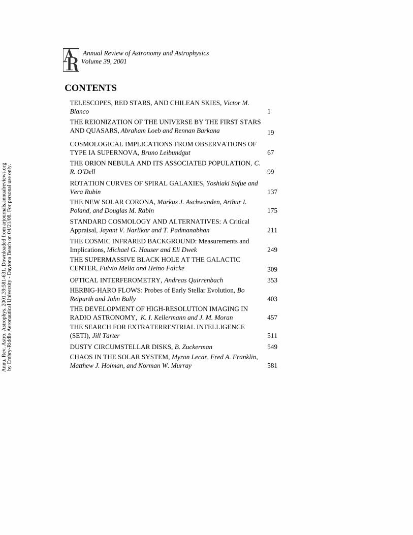
Annual Review of Astronomy and Astrophysics Volume 39, 2001

CONTENTSTELESCOPES, RED STARS, AND CHILEAN SKIES, Victor M. Blanco 1THE REIONIZATION OF THE UNIVERSE BY THE FIRST STARS AND QUASARS, Abraham Loeb and Rennan Barkana 19

COSMOLOGICAL IMPLICATIONS FROM OBSERVATIONS OF TYPE IA SUPERNOVA, Bruno Leibundgut 67THE ORION NEBULA AND ITS ASSOCIATED POPULATION, C. R. O'Dell 99

ROTATION CURVES OF SPIRAL GALAXIES, Yoshiaki Sofue and Vera Rubin 137THE NEW SOLAR CORONA, Markus J. Aschwanden, Arthur I. Poland, and Douglas M. Rabin 175STANDARD COSMOLOGY AND ALTERNATIVES: A Critical Appraisal, Jayant V. Narlikar and T. Padmanabhan 211THE COSMIC INFRARED BACKGROUND: Measurements and Implications, Michael G. Hauser and Eli Dwek 249THE SUPERMASSIVE BLACK HOLE AT THE GALACTIC CENTER, Fulvio Melia and Heino Falcke 309OPTICAL INTERFEROMETRY, Andreas Quirrenbach 353HERBIG-HARO FLOWS: Probes of Early Stellar Evolution, Bo Reipurth and John Bally 403THE DEVELOPMENT OF HIGH-RESOLUTION IMAGING IN RADIO ASTRONOMY, K. I. Kellermann and J. M. Moran 457THE SEARCH FOR EXTRATERRESTRIAL INTELLIGENCE (SETI), Jill Tarter 511

DUSTY CIRCUMSTELLAR DISKS, B. Zuckerman 549CHAOS IN THE SOLAR SYSTEM, Myron Lecar, Fred A. Franklin, Matthew J. Holman, and Norman W. Murray 581

Ann

u. R

ev. A

stro

. Ast

roph

ys. 2

001.

39:5

81-6

31. D

ownl

oade

d fr

om a

rjou

rnal

s.an

nual

revi

ews.

org

by E

mbr

y-R

iddl

e A

eron

autic

al U

nive

rsity

- D

ayto

na B

each

on

04/2

1/08

. For

per

sona

l use

onl

y.

Documents

CHAOS IN THE SOLAR SYSTEM1 - Embry–Riddle …pages.erau.edu/~reynodb2/ep393/Chaos_SolarSystem.pdf · CHAOS IN THE SOLAR SYSTEM 583 Itisnottooalarmingthatsmallbodiesbehavechaotically.Cometsandasteroids