Chaos as an Intermittently Forced Linear SystemSteven L. Brunton1∗, Bingni W. Brunton2, Joshua L. Proctor3, Eurika Kaiser1, J. Nathan Kutz4

1 Department of Mechanical Engineering, University of Washington, Seattle, WA 98195, United States2 Department of Biology, University of Washington, Seattle, WA 98195, United States

3Institute for Disease Modeling, Bellevue, WA 98004, United States4 Department of Applied Mathematics, University of Washington, Seattle, WA 98195, United States

Abstract

Understanding the interplay of order and disorder in chaotic systems is a central challengein modern quantitative science. We present a universal, data-driven decomposition of chaosas an intermittently forced linear system. This work combines Takens’ delay embedding withmodern Koopman operator theory and sparse regression to obtain linear representations ofstrongly nonlinear dynamics. The result is a decomposition of chaotic dynamics into a linearmodel in the leading delay coordinates with forcing by low energy delay coordinates; we callthis the Hankel alternative view of Koopman (HAVOK) analysis. This analysis is applied to thecanonical Lorenz system, as well as to real-world examples such as the Earth’s magnetic fieldreversal, and data from electrocardiogram, electroencephalogram, and measles outbreaks. Ineach case, the forcing statistics are non-Gaussian, with long tails corresponding to rare eventsthat trigger intermittent switching and bursting phenomena; this forcing is highly predictive,providing a clear signature that precedes these events. Moreover, the activity of the forcing sig-nal demarcates large coherent regions of phase space where the dynamics are approximatelylinear from those that are strongly nonlinear.

Keywords– Dynamical systems, Chaos, Data-driven models, Time delays, Koopman analysis.

1 Introduction

Dynamical systems describe the world around us, modeling the interactions between quantitiesthat co-evolve in time [40]. These dynamics often give rise to rich and complex behaviors that maybe difficult to predict from uncertain measurements, a phenomena that is commonly known aschaos. Chaotic dynamics are ubiquitous in the physical, biological, and engineering sciences, andthey have captivated amateurs and experts alike for over a century. The motion of planets [76],weather and climate [63, 65, 66, 38, 83, 67], population dynamics [9, 94, 102], epidemiology [93],financial markets, earthquakes, solar flares, and turbulence [53, 51, 52, 95, 12], all provide com-pelling examples of chaos. Despite the name, chaos is not random, but is instead highly organized,exhibiting coherent structure and patterns [97, 24].

The confluence of big data and advanced algorithms in machine learning is driving a paradigmshift in the analysis and understanding of dynamical systems in science and engineering. Dataare abundant, while physical laws or governing equations remain elusive, as is true for prob-lems in climate science, finance, and neuroscience. Even in classical fields such as turbulence,where governing equations do exist, researchers are increasingly turning towards data-drivenanalysis [83, 67, 12]. Many critical data-driven problems, such as predicting climate change, un-derstanding cognition from neural recordings, or controlling turbulence for energy efficient power

∗ Corresponding author (sbrunton@uw.edu).Matlab code: http://faculty.washington.edu/sbrunton/HAVOK.zipVideo abstract: http://youtu.be/831Ell3QNck

1

arX

iv:1

608.

0530

6v1

[m

ath.

DS]

18

Aug

201

6

production and transportation, are primed to take advantage of progress in the data-driven dis-covery of dynamics [88, 13].

An early success of data-driven dynamical systems is the celebrated Takens embedding theo-rem [95], which allows for the reconstruction of an attractor that is diffeomorphic to the originalchaotic attractor from a time series of a single measurement. This remarkable result states that,under certain conditions, the full dynamics of a system as complicated as a turbulent fluid may beuncovered from a time series of a single point measurement. Delay embedding has been widelyused to analyze and characterize chaotic systems [30, 25, 93, 81, 1, 94, 102], as well as for linearsystem identification with the eigensystem realization algorithm (ERA) [44] and in climate sci-ence with the singular spectrum analysis (SSA) [11] and nonlinear Laplacian spectrum analysis(NLSA) [38]. Until now, there has been a disconnect between the use of delay embeddings tocharacterize chaos and their rigorous use to identify models of the nonlinear dynamics.

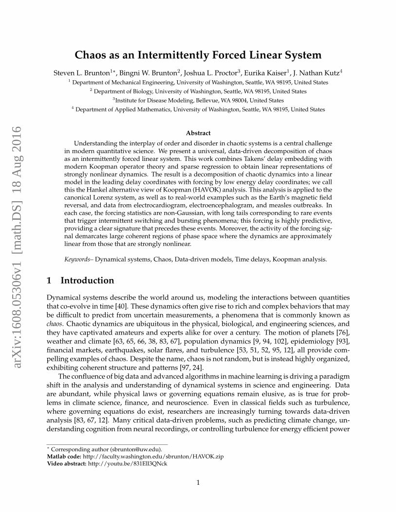
Historically, the two dominant perspectives on dynamical systems have either been geometricor statistical [18]. In the geometric perspective, illustrated in Fig. 1, the organization and topologyof trajectories in phase space provides a qualitative picture of global dynamics and enables de-tailed quantitative descriptions of local dynamics near fixed points or periodic orbits [40, 68, 2, 20,69, 54]. Phase space transport is largely mediated by saddle points, and even in relatively simplesystems such as the double pendulum or Lorenz system in Fig. 1, the dynamics may give riseto chaotic dynamics. The statistical perspective trades the analysis of a single trajectory with thedescription of an ensemble of trajectories, providing a notion of mixing and uncertainty, while bal-ancing the apparent structure and disorder in chaotic systems [26, 27, 28, 32, 33, 31, 45]. Recently,a third operator-theoretic perspective, based on the evolution of measurement functions of the sys-tem, is gaining traction. This approach is not new, being introduced in 1931 by Koopman [55],although the recent deluge of measurement data has renewed interest.

Here, we develop a universal data-driven decomposition of chaos into a forced linear sys-tem. This relies on time-delay embedding, a cornerstone of dynamical systems, but takes a newperspective based on regression models [13] and modern Koopman operator theory [70, 71, 37].The resulting method partitions phase space into coherent regions where the forcing is small anddynamics are approximately linear, and regions where the forcing is large. The forcing may bemeasured from time series data and strongly predicts attractor switching and bursting phenom-ena in real-world examples. Linear representations of strongly nonlinear dynamics, enabled bymachine learning and Koopman theory, promise to transform our ability to estimate, predict, andcontrol complex systems in many diverse fields.

Increasing Nonlinearity

Linear Weakly Nonlinear Chaotic

Increasing Complexity

Linear Weakly Nonlinear Chaotic

Figure 1: Chaotic dynamical systems are often viewed as a progression of increasing nonlinearity.

2

2 Background

The results in this paper are presented in the context of modern dynamical systems, specifically interms of the Koopman operator. In this section, we provide a brief overview of relevant conceptsin dynamical systems, including a discussion of Koopman operator theory in Sec. 2.1, data-drivendynamical systems regression techniques in Sec. 2.2.1, and delay embedding theory in Sec. 2.3.

Throughout this work, we will consider dynamical systems of the form:

d

dtx(t) = f(x(t)). (1)

We will also consider the induced discrete-time dynamical system

xk+1 = F(xk) (2)

where xk may be obtained by sampling the trajectory in Eq. (1) discretely in time, so that xk = x(k∆t).The discrete-time propagator F is given by the flow map

F(xk) = xk +

∫ (k+1)∆t

k∆tf(x(τ)) dτ. (3)

The discrete-time perspective is often more natural when considering experimental data.

2.1 Koopman operator theory

Koopman spectral analysis was introduced in 1931 by B. O. Koopman [55] to describe the evolu-tion of measurements of Hamiltonian systems, and this theory was generalized in 1932 by Koop-man and von Neumann to systems with continuous spectra [56]. Koopman analysis providesan alternative to the more common geometric and statistical perspectives, instead describing theevolution operator that advances the space of measurement functions of the state of the dynam-ical system. The Koopman operator K is an infinite-dimensional linear operator that advancesmeasurement functions g of the state x forward in time according to the dynamics in (2):

Kg , g ◦ F =⇒ Kg(xk) = g(xk+1). (4)

Because this is true for all measurement functions g, K is infinite dimensional and acts on theHilbert space of functions of the state. For a detailed discussion on the Koopman operator, thereare many excellent research articles [70, 82, 16, 17, 61] and reviews [18, 71].

A linear description of nonlinear dynamics is appealing, as many powerful analytic techniquesexist to decompose, advance, and control linear systems. However, the Koopman frameworktrades finite-dimensional nonlinear dynamics for infinite-dimensional linear dynamics. Asidefrom a few notable exceptions [35, 7], it is rare to obtain analytical representations of the Koopmanoperator. Obtaining a finite-dimensional approximation (i.e., a matrix K) of the Koopman opera-tor is therefore an important goal of data-driven analysis and control; this relies on a measurementsubspace that remains invariant to the Koopman operator [15]. Consider a measurement subspacespanned by measurement functions {g1, g2, . . . , gp} so that for any measurement g in this subspace

g = α1g1 + α2g2 + · · ·+ αpgp (5)

then it remains in the subspace after being acted on by the Koopman operator

Kg = β1g1 + β2g2 + · · ·+ βpgp. (6)

3

x1

x2 x3 xN

yNy3y2

y1

gM

KFRp

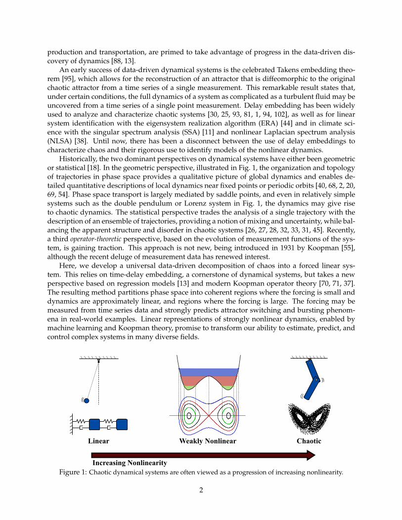
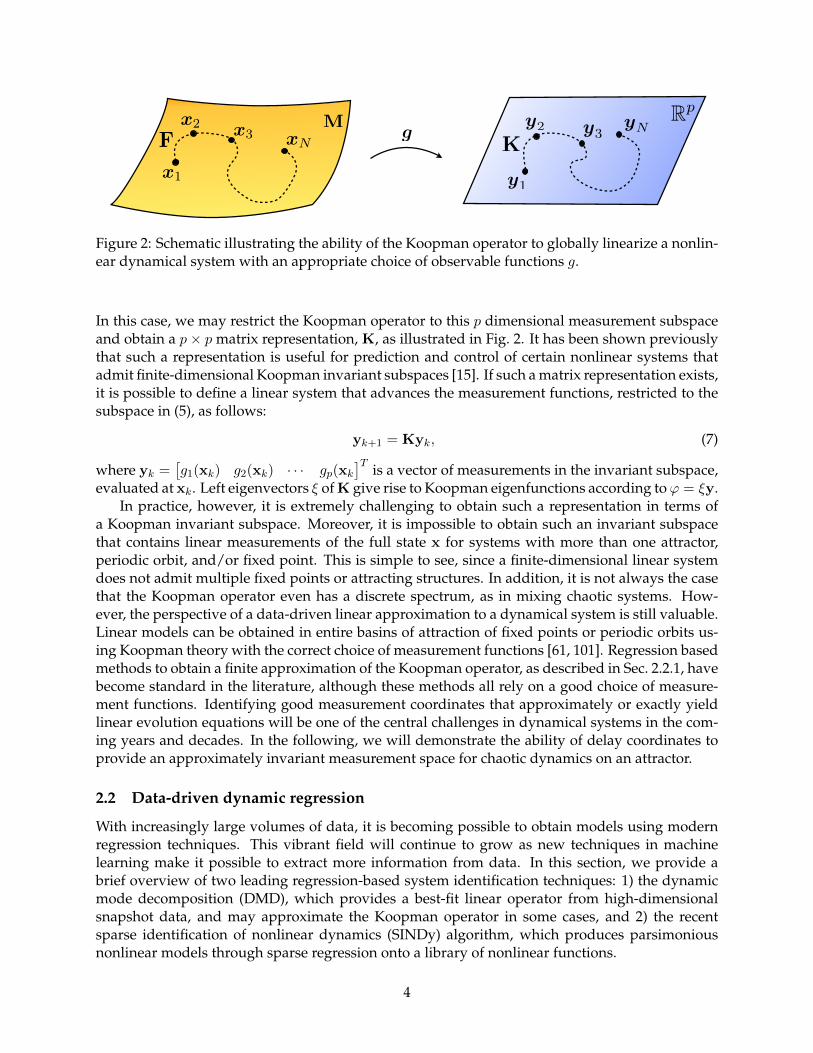
Figure 2: Schematic illustrating the ability of the Koopman operator to globally linearize a nonlin-ear dynamical system with an appropriate choice of observable functions g.

In this case, we may restrict the Koopman operator to this p dimensional measurement subspaceand obtain a p× p matrix representation, K, as illustrated in Fig. 2. It has been shown previouslythat such a representation is useful for prediction and control of certain nonlinear systems thatadmit finite-dimensional Koopman invariant subspaces [15]. If such a matrix representation exists,it is possible to define a linear system that advances the measurement functions, restricted to thesubspace in (5), as follows:

yk+1 = Kyk, (7)

where yk =[g1(xk) g2(xk) · · · gp(xk

]T is a vector of measurements in the invariant subspace,evaluated at xk. Left eigenvectors ξ of K give rise to Koopman eigenfunctions according toϕ = ξy.

In practice, however, it is extremely challenging to obtain such a representation in terms ofa Koopman invariant subspace. Moreover, it is impossible to obtain such an invariant subspacethat contains linear measurements of the full state x for systems with more than one attractor,periodic orbit, and/or fixed point. This is simple to see, since a finite-dimensional linear systemdoes not admit multiple fixed points or attracting structures. In addition, it is not always the casethat the Koopman operator even has a discrete spectrum, as in mixing chaotic systems. How-ever, the perspective of a data-driven linear approximation to a dynamical system is still valuable.Linear models can be obtained in entire basins of attraction of fixed points or periodic orbits us-ing Koopman theory with the correct choice of measurement functions [61, 101]. Regression basedmethods to obtain a finite approximation of the Koopman operator, as described in Sec. 2.2.1, havebecome standard in the literature, although these methods all rely on a good choice of measure-ment functions. Identifying good measurement coordinates that approximately or exactly yieldlinear evolution equations will be one of the central challenges in dynamical systems in the com-ing years and decades. In the following, we will demonstrate the ability of delay coordinates toprovide an approximately invariant measurement space for chaotic dynamics on an attractor.

2.2 Data-driven dynamic regression

With increasingly large volumes of data, it is becoming possible to obtain models using modernregression techniques. This vibrant field will continue to grow as new techniques in machinelearning make it possible to extract more information from data. In this section, we provide abrief overview of two leading regression-based system identification techniques: 1) the dynamicmode decomposition (DMD), which provides a best-fit linear operator from high-dimensionalsnapshot data, and may approximate the Koopman operator in some cases, and 2) the recentsparse identification of nonlinear dynamics (SINDy) algorithm, which produces parsimoniousnonlinear models through sparse regression onto a library of nonlinear functions.

4

2.2.1 Dynamic mode decomposition (DMD)

Dynamic mode decomposition (DMD) was originally introduced in the fluid dynamics commu-nity to decompose large experimental or numerical data sets into leading spatiotemporal coherentstructures [87, 86]. Shortly after, it was shown that the DMD algorithm provides a practical numer-ical framework to approximate the Koopman mode decomposition [82]. This connection betweenDMD and the Koopman operator was further strengthened and justified in a dynamic regressionframework [19, 98, 58].

The DMD algorithm seeks a best-fit linear model to relate the following two data matrices

X =

x1 x2 · · · xm−1

X′ =

x2 x3 · · · xm

. (8)

The matrix X contains snapshots of the system state in time, and X′ is a matrix of the same snap-shots advanced a single step forward in time. These matrices may be related by a best-fit linearoperator A given by

X′ = AX =⇒ A ≈ X′X†, (9)

where X† is the pseudo-inverse, obtained via the singular value decomposition (SVD). The matrixA is a best-fit linear operator in the sense that it minimizes the Frobenius norm error ‖X′−AX‖F .

For systems of moderately large dimension, the operator A is intractably large, and so insteadof obtaining A directly, we often seek the leading eigendecomposition of A:

1. Take the SVD of X:

X = UΣV∗. (10)

Here, ∗ denotes complex conjugate transpose. Often, only the first r columns of U and V arerequired for a good approximation, X ≈ UΣV, where˜denotes a rank-r truncation.

2. Obtain the r × r matrix A by projecting A onto U:

A = U∗AU = U∗X′VΣ−1. (11)

3. Compute the eigendecomposition of A:

AW = WΛ. (12)

The eigenvalues in Λ are eigenvalues of the full matrix A.

4. Reconstruct full-dimensional eigenvectors of A, given by the columns of Φ:

Φ = X′VΣ−1W. (13)

DMD, in its original formulation, is based on linear measurements of the state x of the system,such as velocity measurements from particle image velocimetry (PIV). This means that the mea-surement function g is the identity map on the state. Linear measurements are not rich enoughfor many nonlinear dynamical systems, and so DMD has recently been extended to an augmentedmeasurement vector including nonlinear functions of the state [101]. However, choosing the cor-rect nonlinear measurements that result in an approximately closed Koopman-invariant measure-ment system is still an open problem. Typically, measurement functions are either determinedusing information from the dynamical system (i.e., using quadratic nonlinearities for the Navier-Stokes equations), or by a brute-force search in a particular basis of Hilbert space (i.e., searchingfor polynomial functions or radial basis functions).

5

2.2.2 Sparse identification of nonlinear dynamics (SINDy)

A recently developed technique, the sparse identification of nonlinear dynamics (SINDy) algo-rithm, identifies the nonlinear dynamics in Eq. (1) from measurement data [13]. The SINDy algo-rithm uses sparse regression [96] in a nonlinear function space to determine the few active termsin the dynamics. Earlier related methods based on compressed sensing have been used to pre-dict catastrophes in dynamical systems [99]. There are alternative methods that employ symbolicregression (i.e., genetic programming [57]) to identify dynamics [10, 88]. This work is part of agrowing literature that is exploring the use of sparsity in dynamics [72, 84, 64] and dynamicalsystems [8, 78, 14].

The SINDy algorithm is an equation-free method [50] to identify a dynamical system (1) fromdata, much as in the DMD algorithm above. The basis of the SINDy algorithm is the observationthat for many systems of interest, the function f only has a few active terms, making it sparse inthe space of possible functions. Instead of performing a brute-force search for the active terms inthe dynamics, sparse regression makes it possible to efficiently identify the few non-zero terms.

To determine the function f from data, we collect a time-history of the state x(t) and the deriva-tive x(t); note that x(t) may be approximated numerically from x. The data is sampled at severaltimes t1, t2, · · · , tm and arranged into two large matrices:

X =

state−−−−−−−−−−−−−−−−−−−−−−−−→

x1(t1) x2(t1) · · · xn(t1)x1(t2) x2(t2) · · · xn(t2)

......

. . ....

x1(tm) x2(tm) · · · xn(tm)

y

time

X =

x1(t1) x2(t1) · · · xn(t1)x1(t2) x2(t2) · · · xn(t2)

......

. . ....

x1(tm) x2(tm) · · · xn(tm)

. (14a)

Next, we construct an augmented library Θ(X) consisting of candidate nonlinear functions of thecolumns of X. For example, Θ(X) may consist of constant, polynomial and trigonometric terms:

Θ(X) =

1 X XP2 XP3 · · · sin(X) cos(X) sin(2X) cos(2X) · · ·

. (15)

Each column of Θ(X) is a candidate function for the right hand side of Eq. (1). Since only afew of these nonlinearities are likely active in each row of f , sparse regression is used to determinethe sparse vectors of coefficients Ξ =

[ξ1 ξ2 · · · ξn

]indicating which nonlinearities are active.

X = Θ(X)Ξ. (16)

Once Ξ has been determined, a model of each row of the governing equations may be con-structed as follows:

xk = fk(x) = Θ(xT )ξk. (17)

We may solve for Ξ in Eq. (16) using sparse regression. In many cases, we may need to normal-ize the columns of Θ(X) first to ensure that the restricted isometry property holds [99]; this isespecially important when the entries in X are small, since powers of X will be minuscule.

Note that in the case the the library Θ contains linear measurements of the state, the SINDymethod reduces to a linear regression, closely related to the DMD above, but with transposednotation. The SINDy algorithm also generalizes naturally to discrete-time formulations.

6

2.3 Time-delay embedding

It has long been observed that choosing good measurements is critical to modeling, predicting,and controlling dynamical systems. The concept of observability in a linear dynamical systemprovides conditions for when the full-state of a system may be estimated from a time-historyof measurements of the system, providing a rigorous foundation for dynamic estimation, suchas the Kalman filter [46, 43, 100, 29, 91]. Although observability has been extended to nonlinearsystems [42], significantly fewer results hold in this more general context.

The Takens embedding theorem [95] provides a rigorous framework for analyzing the infor-mation content of measurements of a nonlinear dynamical system. It is possible to enrich a mea-surement, x(t), with time-shifted copies of itself, x(t− τ), which are known as delay coordinates.Under certain conditions, the attractor of a dynamical system in delay coordinates is diffeomorphicto the original attractor in the original state space. This is truly remarkable, as this theory statesthat in some cases, it may be possible to reconstruct the entire attractor of a turbulent fluid froma time series of a single point measurement. Similar differential embeddings may be constructedby using derivatives of the measurement. Takens embedding theory has been related to nonlinearobservability [4, 5], providing a much needed connection between these two important fields.

Delay embedding has been widely used to analyze and characterize chaotic systems [30, 25,93, 81, 1, 94, 102]. The use of generalized delay coordinates are also used for linear system iden-tification with the eigensystem realization algorithm (ERA) [44] and in climate science with thesingular spectrum analysis (SSA) [11] and nonlinear Laplacian spectrum analysis (NLSA) [38].All of these methods are based on a singular value decomposition of a Hankel matrix, which isdiscussed below.

2.3.1 Hankel matrix analysis

Both the eigensystem realization algorithm (ERA) [44] and the singular spectrum analysis (SSA) [11]are based on the construction of a Hankel matrix from a time series of measurement data. In thefollowing, we will present the theory for a single scalar measurement, although this frameworkgeneralizes to multiple input, multiple output (MIMO) problems.

The following Hankel matrix H is formed from a time series of a measurement y(t):

H =

y(t1) y(t2) · · · y(tp)y(t2) y(t3) · · · y(tp+1)

......

. . ....

y(tq) y(tq+1) · · · y(tm)

. (18)

Taking the singular value decomposition (SVD) of the Hankel matrix,

H = UΣVT , (19)

yields a hierarchical decomposition of the matrix into eigen time series given by the columns ofU and V. These columns are ordered by their ability to express the variance in the columns androws of the matrix H, respectively. When the measurement y(t) comes from the impulse responseof an observable linear system, then it is possible to use the SVD of the matrix H to reconstruct anaccurate model of the full dynamics. This ERA procedure is widely used in system identification,and it has been recently connected to DMD [98, 79]. In the following, we will generalize systemidentification using the Hankel matrix to nonlinear dynamical systems via the Koopman analysis.

7

3 Decomposing chaos: Hankel alternative view of Koopman (HAVOK)

Obtaining linear representations for strongly nonlinear systems has the potential to revolutionizeour ability to predict and control these systems. In fact, the linearization of dynamics near fixedpoints or periodic orbits has long been employed for local linear representation of the dynam-ics [40]. The Koopman operator is appealing because it provides a global linear representation,valid far away from fixed points and periodic orbits, although previous attempts to obtain finite-dimensional approximations of the Koopman operator have had limited success. Dynamic modedecomposition (DMD) [86, 82, 58] seeks to approximate the Koopman operator with a best-fit lin-ear model advancing spatial measurements from one time to the next. However, DMD is based onlinear measurements, which are not rich enough for many nonlinear systems. Augmenting DMDwith nonlinear measurements may enrich the model, but there is no guarantee that the resultingmodels will be closed under the Koopman operator [15].

Instead of advancing instantaneous measurements of the state of the system, we obtain intrin-sic measurement coordinates based on the time-history of the system. This perspective is data-driven, relying on the wealth of information from previous measurements to inform the future.Unlike a linear or weakly nonlinear system, where trajectories may get trapped at fixed pointsor on periodic orbits, chaotic dynamics are particularly well-suited to this analysis: trajectoriesevolve to densely fill an attractor, so more data provides more information.

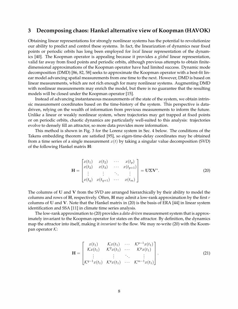
This method is shown in Fig. 3 for the Lorenz system in Sec. 4 below. The conditions of theTakens embedding theorem are satisfied [95], so eigen-time-delay coordinates may be obtainedfrom a time series of a single measurement x(t) by taking a singular value decomposition (SVD)of the following Hankel matrix H:

H =

x(t1) x(t2) · · · x(tp)x(t2) x(t3) · · · x(tp+1)

......

. . ....

x(tq) x(tq+1) · · · x(tm)

= UΣV∗. (20)

The columns of U and V from the SVD are arranged hierarchically by their ability to model thecolumns and rows of H, respectively. Often, H may admit a low-rank approximation by the first rcolumns of U and V. Note that the Hankel matrix in (20) is the basis of ERA [44] in linear systemidentification and SSA [11] in climate time series analysis.

The low-rank approximation to (20) provides a data-driven measurement system that is approx-imately invariant to the Koopman operator for states on the attractor. By definition, the dynamicsmap the attractor into itself, making it invariant to the flow. We may re-write (20) with the Koom-pan operator K:

H =

x(t1) Kx(t1) · · · Kp−1x(t1)Kx(t1) K2x(t1) · · · Kpx(t1)

......

. . ....

Kq−1x(t1) Kqx(t1) · · · Km−1x(t1)

. (21)

8

The columns of (20), and thus (21), are well-approximated by the first r columns of U, so theseeigen time series provide a Koopman-invariant measurement system. The first r columns of Vprovide a time series of the magnitude of each of the columns of UΣ in the data. By plotting thefirst three columns of V, we obtain an embedded attractor for the Lorenz system, shown in Fig. 3.The rank r can be obtained by the optimal hard threshold of Gavish and Donoho [36] or by otherattractor dimension arguments [1].

The connection between eigen-time-delay coordinates from (20) and the Koopman operatormotivates a linear regression model on the variables in V. Even with an approximately Koopman-invariant measurement system, there remain challenges to identifying a linear model for a chaoticsystem. A linear model, however detailed, cannot capture multiple fixed points or the unpre-dictable behavior characteristic of chaos with a positive Lyapunov exponent [15]. Instead of con-structing a closed linear model for the first r variables in V, we build a linear model on the firstr − 1 variables and impose the last variable, vr, as a forcing term.

d

dtv(t) = Av(t) + Bvr(t), (22)

where v =[v1 v2 · · · vr−1

]T is a vector of the first r − 1 eigen-time-delay coordinates. In allof the examples below, the linear model on the first r − 1 terms is accurate, while no linear modelrepresents vr. Instead, vr is an input forcing to the linear dynamics in (22), which approximate thenonlinear dynamics in (1). The statistics of vr(t) are non-Gaussian, as seen in the lower-right panelin Fig. 3. The long tails correspond to rare-event forcing that drives lobe switching in the Lorenzsystem; this is related to rare-event forcing distributions observed and modeled by others [66, 83,67].

The forced linear system in (22) was discovered after applying the sparse identification of non-linear dynamics (SINDy) [13] algorithm to delay coordinates of the Lorenz system. Even whenallowing for the possibility of nonlinear dynamics for v, the most parsimonious model was linearwith a dominant off-diagonal structure in the A matrix (shown in Fig. ??). This strongly sug-gests a connection with the Koopman operator, motivating the present work. The last term vr isnot accurately represented by either linear or polynomial nonlinear models [13]. We refer to theframework presented here as the Hankel alternative view of Koopman (HAVOK) analysis.

The HAVOK analysis will be explored in detail below on the Lorenz system in Sec. 4 and on awide range of numerical, experimental, and historical data models in Sec. 5. In nearly all of theseexamples, the forcing is generally small except for intermittent punctate events that correspondto transient attractor switching (for example, lobe switching in the Lorenz system) or burstingphenomena (in the case of Measles outbreaks). When the forcing signal is small, the dynamics arewell-described by the Koopman linear system on the data-driven delay coordinates. When theforcing is large, the system is driven by an essential nonlinearity, which typically corresponds toan intermittent switching or bursting event. The regions of small and large forcing correspondto large coherent regions of phase space that may be analyzed further through machine learningtechniques.

9

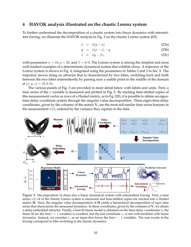
4 HAVOK analysis illustrated on the chaotic Lorenz system

To further understand the decomposition of a chaotic system into linear dynamics with intermit-tent forcing, we illustrate the HAVOK analysis in Fig. 3 on the chaotic Lorenz system [63]:

x = σ(y − x) (23a)y = x(ρ− z)− y (23b)z = xy − βz, (23c)

with parameters σ = 10, ρ = 28, and β = 8/3. The Lorenz system is among the simplest and mostwell-studied examples of a deterministic dynamical system that exhibits chaos. A trajectory of theLorenz system is shown in Fig. 4, integrated using the parameters in Tables 2 and 3 in Sec. 5. Thetrajectory moves along an attractor that is characterized by two lobes, switching back and forthbetween the two lobes intermittently by passing near a saddle point in the middle of the domainat (x, y, z) = (0, 0, 0).

The various panels of Fig. 3 are provided in more detail below with labels and units. First, atime series of the x variable is measured and plotted in Fig. 5. By stacking time-shifted copies ofthis measurement vector as rows of a Hankel matrix, as in Eq. (20), it is possible to obtain an eigen-time-delay coordinate system through the singular value decomposition. These eigen-time-delaycoordinates, given by the columns of the matrix V, are the most self-similar time series features inthe measurement x(t), ordered by the variance they capture in the data.

Decomposing Chaos into Linear Dynamics plus Stochastic Forcing

Steven L. Brunton1⇤, Bingni W. Brunton2, Joshua L. Proctor3, J. Nathan Kutz4

1 Department of Mechanical Engineering, University of Washington, Seattle, WA 98195, United States2 Department of Biology, University of Washington, Seattle, WA 98195, United States

3Institute for Disease Modeling, Bellevue, WA 98004, United States4 Department of Applied Mathematics, University of Washington, Seattle, WA 98195, United States

Abstract

Keywords– Dynamical systems, Chaos, Nonlinear dynamics, Koopman operator, Takens embedding, Timedelay coordinates, Stochastic forcing.

1 Introduction

• Chaos is important: Dynamics [10], Lorenz [14]

• Takens embedding is profound and important [23]

• Connection to Koopman analysis [12]

• Connection to identifying dynamics and DMD [4, 13]

• Koopman invariant subspace [?]

• Time series classics: review [1], book [25]

• ERA [11], SSA [3], NLSA [9]

H =

26664

x(t1) x(t2) x(t3) · · · x(tp)x(t2) x(t3) x(t4) · · · x(tp+1)

......

.... . .

...x(tq) x(tq+1) x(tq+2) · · · x(tm)

37775 (1)

• Dynamics discovery [19]

• Sugihara and time series [21, 26]... old with measles data [22]

• Donoho hard threshold [8]

• Predicting chaotic time series [7]

• Equations from data series [6]

• Extracting dynamics from chaotic data [17]

• Chaos from random[24]

⇤ Corresponding author. Tel.: +1 (609)-921-6415.E-mail address: sbrunton@uw.edu (S.L. Brunton).

1

Delay Embedding

⇥ ⇥

figures/fig_01.pdf

ut = uux + uxxx

• Chaos is important: Dynamics [10], Lorenz [14]

• Takens embedding is profound and important [23]

• Connection to Koopman analysis [12]

• Connection to identifying dynamics and DMD [4, 13]

• Koopman invariant subspace [?]

• Time series classics: review [1], book [25]

• ERA [11], SSA [3], NLSA [9]

H =

26664

x(t1) x(t2) x(t3) · · · x(tr)x(t2) x(t3) x(t4) · · · x(tr+1)

......

.... . .

...x(ts) x(ts+1) x(ts+2) · · · x(tm)

37775 (1)

• Dynamics discovery [19]

• Sugihara and time series [21, 26]... old with measles data [22]

• Donoho hard threshold [8]

• Predicting chaotic time series [7]

• Equations from data series [6]

• Extracting dynamics from chaotic data [17]

2

U ⌃ VT

2666664

v1

v2

v3

...vr

3777775

2666664

v1

v2

v3

...vr

3777775

2666664

v1

v2

v3

...vr

3777775

x

Measure x

Delay Coordinates

Singular Value Decomposition

Intermittent Forcing

Intermittent Switching

Linear Dynamics

2666664

v1

v2

v3

...vr

3777775

d

dt

2666664

v1

v2

v3

...vr

3777775

=

Bad Fit

A B

Regression Model

Gaussianvr

Predicted Attractor

vr

v1

Figure 3: Decomposition of chaos into a linear dynamical system with intermittent forcing. First, a timeseries x(t) of of the chaotic Lorenz system is measured and time-shifted copies are stacked into a Hankelmatrix H. Next, the singular value decomposition of H yields a hierarchical decomposition of eigen timeseries that characterize the measured dynamics. In these coordinates, given by the columns of V, we obtaina delay-embedded attractor. Finally, a best-fit linear model is obtained on the time-delay coordinates v; thelinear fit for the first r − 1 variables is excellent, but the last coordinate vr is not well-modeled with lineardynamics. Instead, we consider vr as an input that forces the first r − 1 variables. The rare events in theforcing correspond to lobe switching in the chaotic dynamics.

10

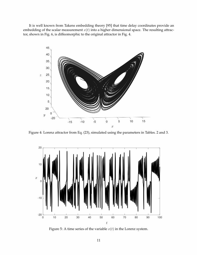
It is well known from Takens embedding theory [95] that time delay coordinates provide anembedding of the scalar measurement x(t) into a higher dimensional space. The resulting attrac-tor, shown in Fig. 6, is diffeomorphic to the original attractor in Fig. 4.

x

y

z

Figure 4: Lorenz attractor from Eq. (23), simulated using the parameters in Tables. 2 and 3.

0 10 20 30 40 50 60 70 80 90 100

-20

-10

0

10

20

t

x

Figure 5: A time series of the variable x(t) in the Lorenz system.

11

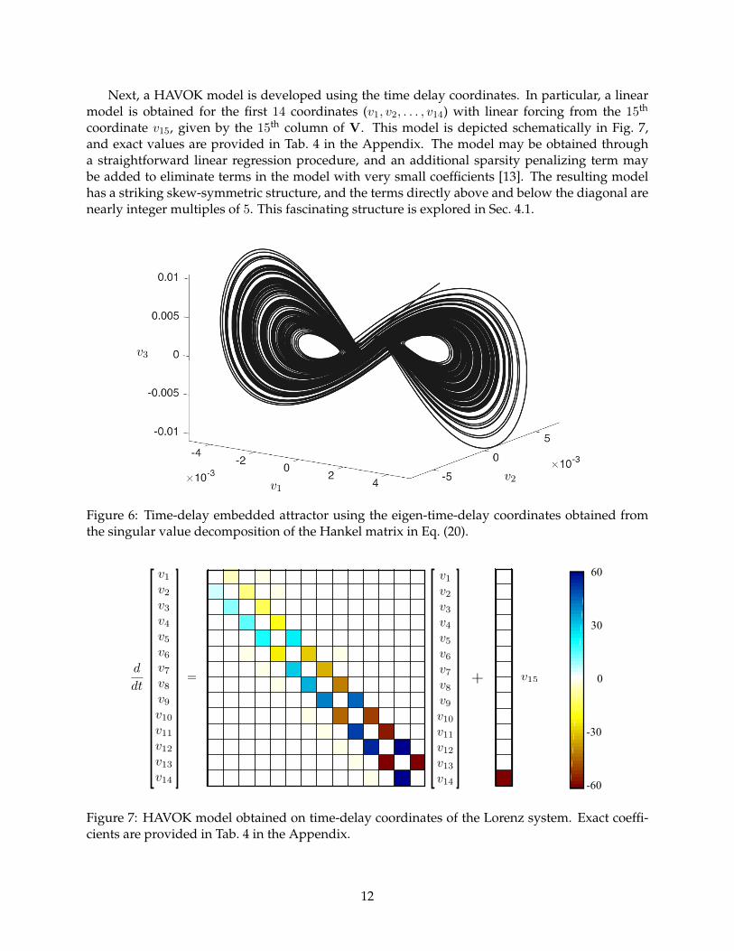
Next, a HAVOK model is developed using the time delay coordinates. In particular, a linearmodel is obtained for the first 14 coordinates (v1, v2, . . . , v14) with linear forcing from the 15th

coordinate v15, given by the 15th column of V. This model is depicted schematically in Fig. 7,and exact values are provided in Tab. 4 in the Appendix. The model may be obtained througha straightforward linear regression procedure, and an additional sparsity penalizing term maybe added to eliminate terms in the model with very small coefficients [13]. The resulting modelhas a striking skew-symmetric structure, and the terms directly above and below the diagonal arenearly integer multiples of 5. This fascinating structure is explored in Sec. 4.1.

v1v2

v3

Figure 6: Time-delay embedded attractor using the eigen-time-delay coordinates obtained fromthe singular value decomposition of the Hankel matrix in Eq. (20).

Convolve with U

2666664

v1

v2

v3

...vr

3777775

Obtain V

0 5 10 15

2

4

6

8

10

12

14

-60

-30

0

30

60

-5 0 5 10

2

4

6

8

10

12

14

d

dt

266666666666666666666664

v1

v2

v3

v4

v5

v6

v7

v8

v9

v10

v11

v12

v13

v14

377777777777777777777775

=

266666666666666666666664

v1

v2

v3

v4

v5

v6

v7

v8

v9

v10

v11

v12

v13

v14

377777777777777777777775

v15+

0 5 10 15

2

4

6

8

10

12

14

-60

-30

0

30

6060

-60

-30

30

0

[

sliding window

d

dt

266666666666666666666664

v1

v2

v3

v4

v5

v6

v7

v8

v9

v10

v11

v12

v13

v14

377777777777777777777775

=d

dt

266666666666666666666664

v1

v2

v3

v4

v5

v6

v7

v8

v9

v10

v11

v12

v13

v14

377777777777777777777775

=

Figure 7: HAVOK model obtained on time-delay coordinates of the Lorenz system. Exact coeffi-cients are provided in Tab. 4 in the Appendix.

12

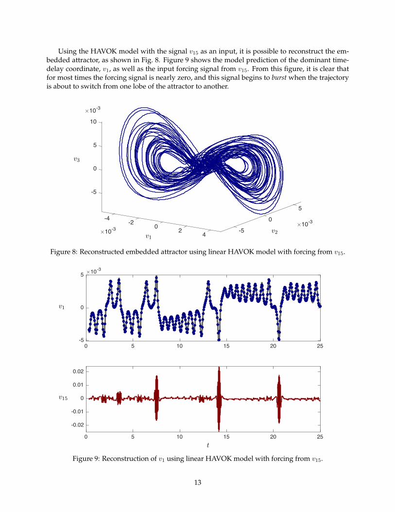
Using the HAVOK model with the signal v15 as an input, it is possible to reconstruct the em-bedded attractor, as shown in Fig. 8. Figure 9 shows the model prediction of the dominant time-delay coordinate, v1, as well as the input forcing signal from v15. From this figure, it is clear thatfor most times the forcing signal is nearly zero, and this signal begins to burst when the trajectoryis about to switch from one lobe of the attractor to another.

5

-5

-4 0×10-3

0

×10-3

-2

5

×10-30

10

2 -54v1v2

v3

Figure 8: Reconstructed embedded attractor using linear HAVOK model with forcing from v15.

0 5 10 15 20 25-5

0

5 ×10-3

0 5 10 15 20 25

-0.02

-0.01

0

0.01

0.02

t

v15

v1

Figure 9: Reconstruction of v1 using linear HAVOK model with forcing from v15.

13

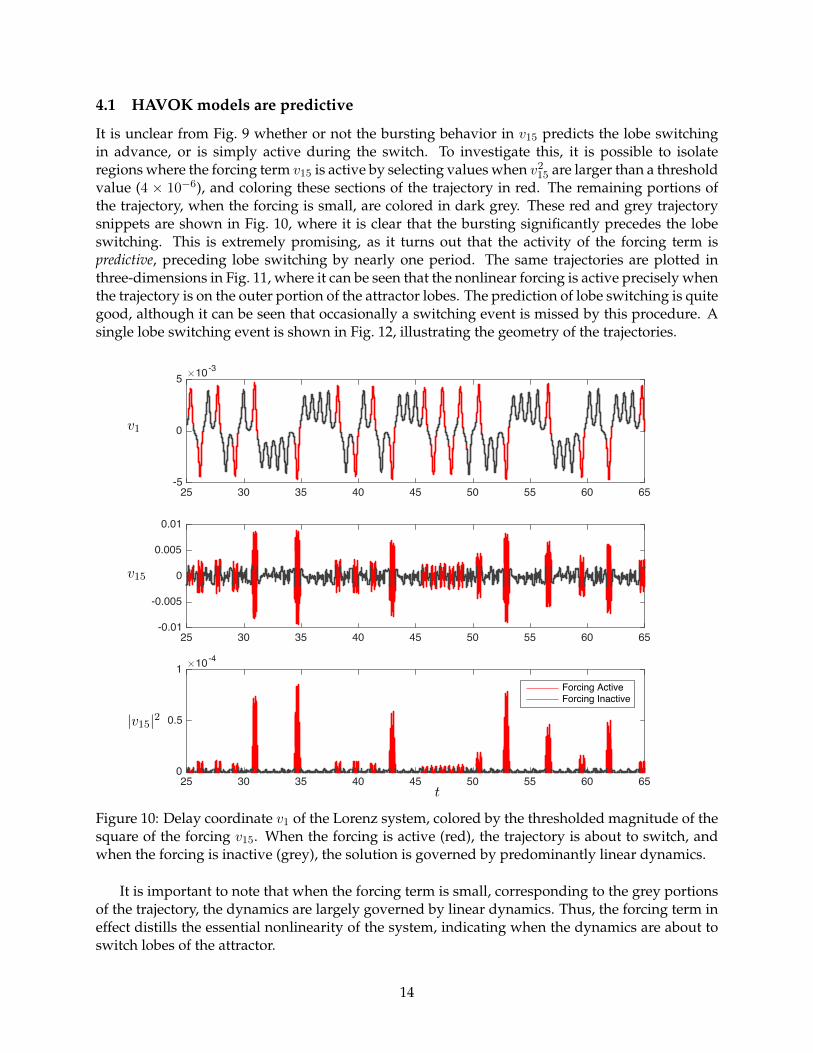
4.1 HAVOK models are predictive

It is unclear from Fig. 9 whether or not the bursting behavior in v15 predicts the lobe switchingin advance, or is simply active during the switch. To investigate this, it is possible to isolateregions where the forcing term v15 is active by selecting values when v2

15 are larger than a thresholdvalue (4 × 10−6), and coloring these sections of the trajectory in red. The remaining portions ofthe trajectory, when the forcing is small, are colored in dark grey. These red and grey trajectorysnippets are shown in Fig. 10, where it is clear that the bursting significantly precedes the lobeswitching. This is extremely promising, as it turns out that the activity of the forcing term ispredictive, preceding lobe switching by nearly one period. The same trajectories are plotted inthree-dimensions in Fig. 11, where it can be seen that the nonlinear forcing is active precisely whenthe trajectory is on the outer portion of the attractor lobes. The prediction of lobe switching is quitegood, although it can be seen that occasionally a switching event is missed by this procedure. Asingle lobe switching event is shown in Fig. 12, illustrating the geometry of the trajectories.

25 30 35 40 45 50 55 60 65-5

0

5 ×10-3

25 30 35 40 45 50 55 60 65-0.01

-0.005

0

0.005

0.01

25 30 35 40 45 50 55 60 650

0.5

1 ×10-4

Forcing ActiveForcing Inactive

t

|v15|2

v15

v1

Figure 10: Delay coordinate v1 of the Lorenz system, colored by the thresholded magnitude of thesquare of the forcing v15. When the forcing is active (red), the trajectory is about to switch, andwhen the forcing is inactive (grey), the solution is governed by predominantly linear dynamics.

It is important to note that when the forcing term is small, corresponding to the grey portionsof the trajectory, the dynamics are largely governed by linear dynamics. Thus, the forcing term ineffect distills the essential nonlinearity of the system, indicating when the dynamics are about toswitch lobes of the attractor.

14

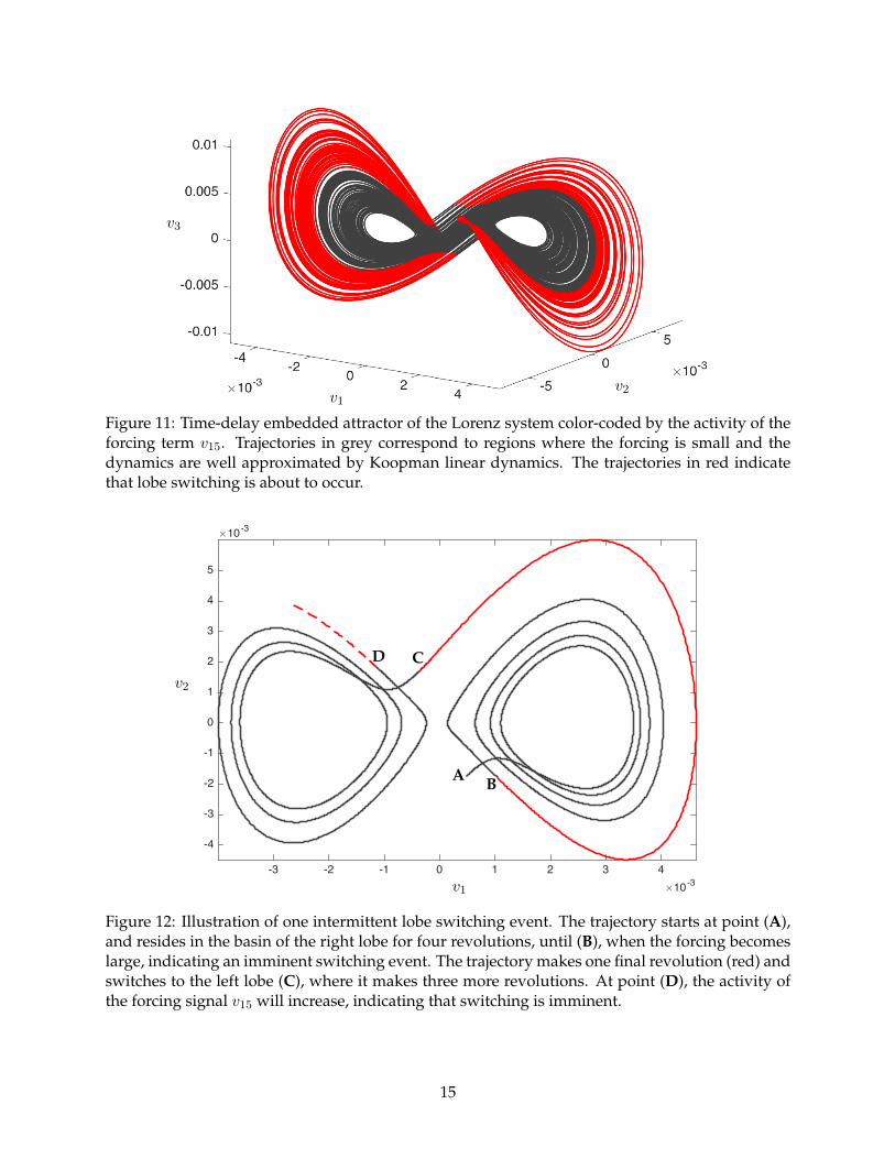
v1v2

v3

Figure 11: Time-delay embedded attractor of the Lorenz system color-coded by the activity of theforcing term v15. Trajectories in grey correspond to regions where the forcing is small and thedynamics are well approximated by Koopman linear dynamics. The trajectories in red indicatethat lobe switching is about to occur.

-3 -2 -1 0 1 2 3 4×10-3

-4

-3

-2

-1

0

1

2

3

4

5

×10-3

v1

v2

A B

CD

Figure 12: Illustration of one intermittent lobe switching event. The trajectory starts at point (A),and resides in the basin of the right lobe for four revolutions, until (B), when the forcing becomeslarge, indicating an imminent switching event. The trajectory makes one final revolution (red) andswitches to the left lobe (C), where it makes three more revolutions. At point (D), the activity ofthe forcing signal v15 will increase, indicating that switching is imminent.

15

0 10 20 30 40 50 60 70 80 90 100

-0.3

-0.2

-0.1

0

0.1

0.2

0.3

r=1

r=2

r=3

r=4

r=5

...

r=15

t

ur

Figure 13: Modes ur (columns of the matrix U), indicating the short-time history that must beconvolved with x(t) to obtain vr.

-0.025 -0.02 -0.015 -0.01 -0.005 0 0.005 0.01 0.015 0.02 0.02510

-4

10-3

10-2

10-1

100

Normal DistributionLorenz Forcing

v15

p

Figure 14: Probability density function of the forcing term in v15 (red), plotted against the proba-bility density function of an appropriately scaled normal distribution (black dash).

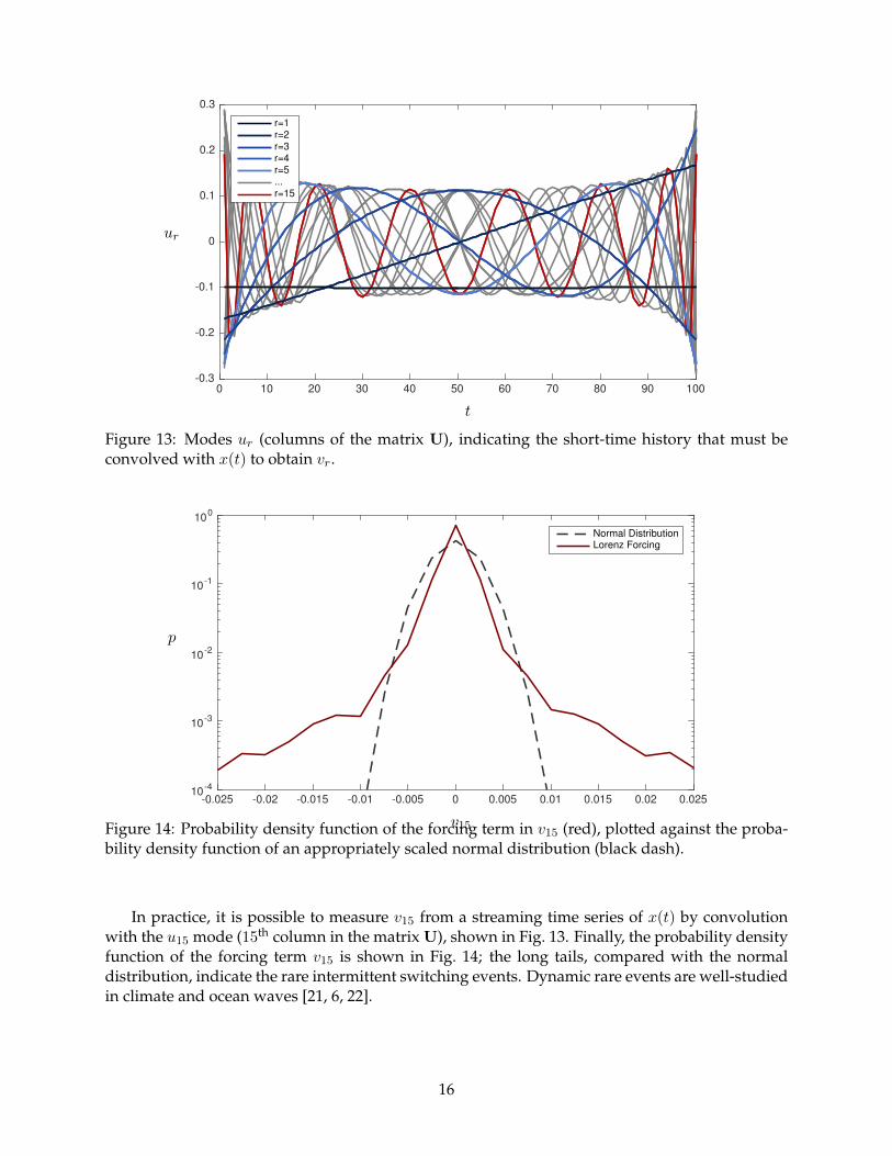
In practice, it is possible to measure v15 from a streaming time series of x(t) by convolutionwith the u15 mode (15th column in the matrix U), shown in Fig. 13. Finally, the probability densityfunction of the forcing term v15 is shown in Fig. 14; the long tails, compared with the normaldistribution, indicate the rare intermittent switching events. Dynamic rare events are well-studiedin climate and ocean waves [21, 6, 22].

16

4.2 HAVOK models generalize beyond training data

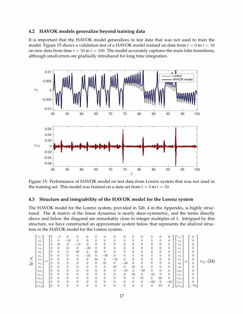
It is important that the HAVOK model generalizes to test data that was not used to train themodel. Figure 15 shows a validation test of a HAVOK model trained on data from t = 0 to t = 50on new data from time t = 50 to t = 100. The model accurately captures the main lobe transitions,although small errors are gradually introduced for long time integration.

50 55 60 65 70 75 80 85 90 95 100-0.01

-0.005

0

0.005

0.01LorenzHAVOK model

50 55 60 65 70 75 80 85 90 95 100

-0.06-0.04-0.02

00.020.040.06

t

v15

v1

Figure 15: Performance of HAVOK model on test data from Lorenz system that was not used inthe training set. This model was trained on a data set from t = 0 to t = 50.

4.3 Structure and integrability of the HAVOK model for the Lorenz system

The HAVOK model for the Lorenz system, provided in Tab. 4 in the Appendix, is highly struc-tured. The A matrix of the linear dynamics is nearly skew-symmetric, and the terms directlyabove and below the diagonal are remarkably close to integer multiples of 5. Intrigued by thisstructure, we have constructed an approximate system below that represents the idealized struc-ture in the HAVOK model for the Lorenz system:

d

dt

v1v2v3v4v5v6v7v8v9v10v11v12v13v14

=

0 −5 0 0 0 0 0 0 0 0 0 0 0 05 0 −10 0 0 0 0 0 0 0 0 0 0 00 10 0 −15 0 0 0 0 0 0 0 0 0 00 0 15 0 −20 0 0 0 0 0 0 0 0 00 0 0 20 0 25 0 0 0 0 0 0 0 00 0 0 0 −25 0 −30 0 0 0 0 0 0 00 0 0 0 0 30 0 −35 0 0 0 0 0 00 0 0 0 0 0 35 0 −40 0 0 0 0 00 0 0 0 0 0 0 40 0 45 0 0 0 00 0 0 0 0 0 0 0 −45 0 −50 0 0 00 0 0 0 0 0 0 0 0 50 0 −55 0 00 0 0 0 0 0 0 0 0 0 55 0 60 00 0 0 0 0 0 0 0 0 0 0 −60 0 −650 0 0 0 0 0 0 0 0 0 0 0 65 0

v1v2v3v4v5v6v7v8v9v10v11v12v13v14

+

0000000000000−70

v15. (24)

17

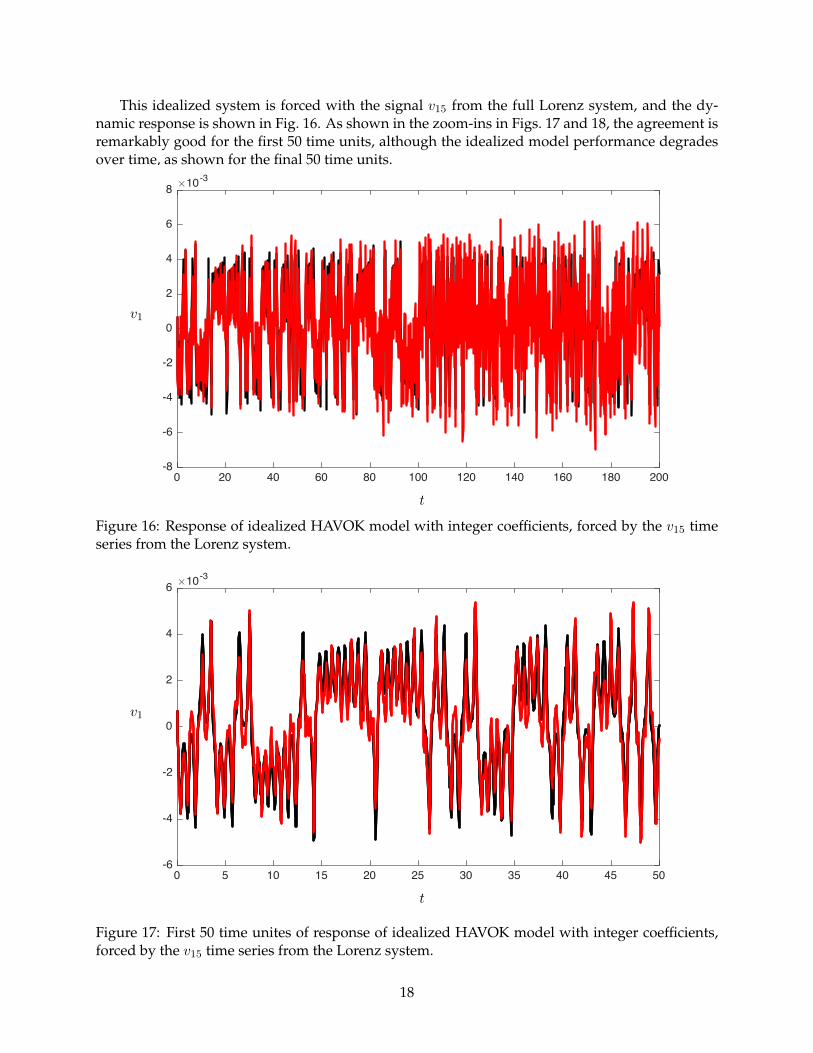
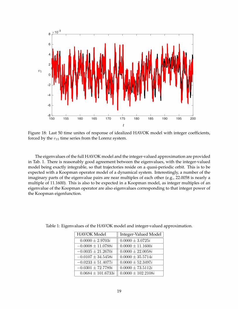
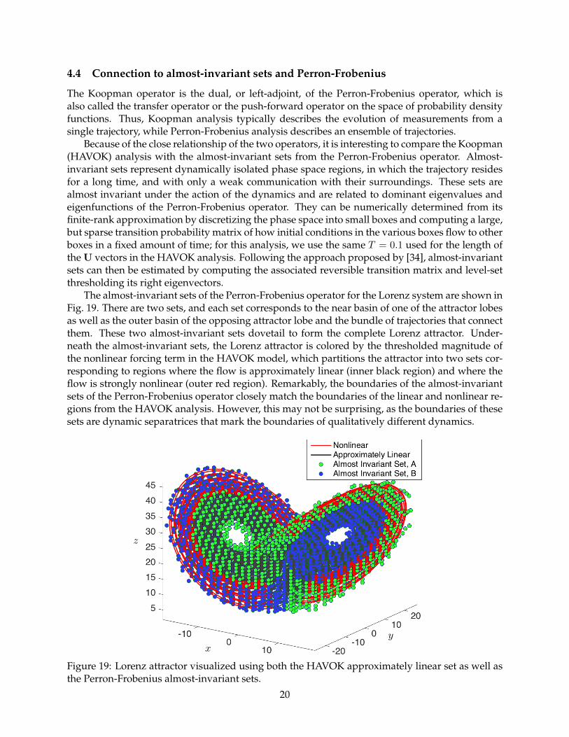
This idealized system is forced with the signal v15 from the full Lorenz system, and the dy-namic response is shown in Fig. 16. As shown in the zoom-ins in Figs. 17 and 18, the agreement isremarkably good for the first 50 time units, although the idealized model performance degradesover time, as shown for the final 50 time units.

0 20 40 60 80 100 120 140 160 180 200-8

-6

-4

-2

0

2

4

6

8 ×10-3

t

v1

Figure 16: Response of idealized HAVOK model with integer coefficients, forced by the v15 timeseries from the Lorenz system.

0 5 10 15 20 25 30 35 40 45 50-6

-4

-2

0

2

4

6 ×10-3

t

v1

Figure 17: First 50 time unites of response of idealized HAVOK model with integer coefficients,forced by the v15 time series from the Lorenz system.

18

150 155 160 165 170 175 180 185 190 195 200-8

-6

-4

-2

0

2

4

6

8 ×10-3

t

v1

Figure 18: Last 50 time unites of response of idealized HAVOK model with integer coefficients,forced by the v15 time series from the Lorenz system.

The eigenvalues of the full HAVOK model and the integer-valued approximation are providedin Tab. 1. There is reasonably good agreement between the eigenvalues, with the integer-valuedmodel being exactly integrable, so that trajectories reside on a quasi-periodic orbit. This is to beexpected with a Koopman operator model of a dynamical system. Interestingly, a number of theimaginary parts of the eigenvalue pairs are near multiples of each other (e.g., 22.0058 is nearly amultiple of 11.1600). This is also to be expected in a Koopman model, as integer multiples of aneigenvalue of the Koopman operator are also eigenvalues corresponding to that integer power ofthe Koopman eigenfunction.

Table 1: Eigenvalues of the HAVOK model and integer-valued approximation.

HAVOK Model Integer-Valued Model0.0000± 2.9703i 0.0000± 3.0725i

−0.0008± 11.0788i 0.0000± 11.1600i

−0.0035± 21.2670i 0.0000± 22.0058i

−0.0107± 34.5458i 0.0000± 35.5714i

−0.0233± 51.4077i 0.0000± 52.3497i

−0.0301± 72.7789i 0.0000± 73.5112i

0.0684± 101.6733i 0.0000± 102.2108i

19

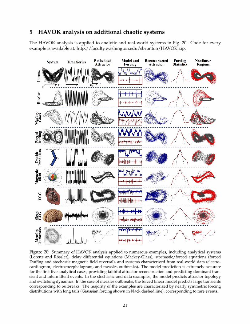
4.4 Connection to almost-invariant sets and Perron-Frobenius

The Koopman operator is the dual, or left-adjoint, of the Perron-Frobenius operator, which isalso called the transfer operator or the push-forward operator on the space of probability densityfunctions. Thus, Koopman analysis typically describes the evolution of measurements from asingle trajectory, while Perron-Frobenius analysis describes an ensemble of trajectories.

Because of the close relationship of the two operators, it is interesting to compare the Koopman(HAVOK) analysis with the almost-invariant sets from the Perron-Frobenius operator. Almost-invariant sets represent dynamically isolated phase space regions, in which the trajectory residesfor a long time, and with only a weak communication with their surroundings. These sets arealmost invariant under the action of the dynamics and are related to dominant eigenvalues andeigenfunctions of the Perron-Frobenius operator. They can be numerically determined from itsfinite-rank approximation by discretizing the phase space into small boxes and computing a large,but sparse transition probability matrix of how initial conditions in the various boxes flow to otherboxes in a fixed amount of time; for this analysis, we use the same T = 0.1 used for the length ofthe U vectors in the HAVOK analysis. Following the approach proposed by [34], almost-invariantsets can then be estimated by computing the associated reversible transition matrix and level-setthresholding its right eigenvectors.

The almost-invariant sets of the Perron-Frobenius operator for the Lorenz system are shown inFig. 19. There are two sets, and each set corresponds to the near basin of one of the attractor lobesas well as the outer basin of the opposing attractor lobe and the bundle of trajectories that connectthem. These two almost-invariant sets dovetail to form the complete Lorenz attractor. Under-neath the almost-invariant sets, the Lorenz attractor is colored by the thresholded magnitude ofthe nonlinear forcing term in the HAVOK model, which partitions the attractor into two sets cor-responding to regions where the flow is approximately linear (inner black region) and where theflow is strongly nonlinear (outer red region). Remarkably, the boundaries of the almost-invariantsets of the Perron-Frobenius operator closely match the boundaries of the linear and nonlinear re-gions from the HAVOK analysis. However, this may not be surprising, as the boundaries of thesesets are dynamic separatrices that mark the boundaries of qualitatively different dynamics.

y

x

z

Figure 19: Lorenz attractor visualized using both the HAVOK approximately linear set as well asthe Perron-Frobenius almost-invariant sets.

20

5 HAVOK analysis on additional chaotic systems

The HAVOK analysis is applied to analytic and real-world systems in Fig. 20. Code for everyexample is available at: http://faculty.washington.edu/sbrunton/HAVOK.zip.

Figure 20: Summary of HAVOK analysis applied to numerous examples, including analytical systems(Lorenz and Rossler), delay differential equations (Mackey-Glass), stochastic/forced equations (forcedDuffing and stochastic magnetic field reversal), and systems characterized from real-world data (electro-cardiogram, electroencephalogram, and measles outbreaks). The model prediction is extremely accuratefor the first five analytical cases, providing faithful attractor reconstruction and predicting dominant tran-sient and intermittent events. In the stochastic and data examples, the model predicts attractor topologyand switching dynamics. In the case of measles outbreaks, the forced linear model predicts large transientscorresponding to outbreaks. The majority of the examples are characterized by nearly symmetric forcingdistributions with long tails (Gaussian forcing shown in black dashed line), corresponding to rare events.

21

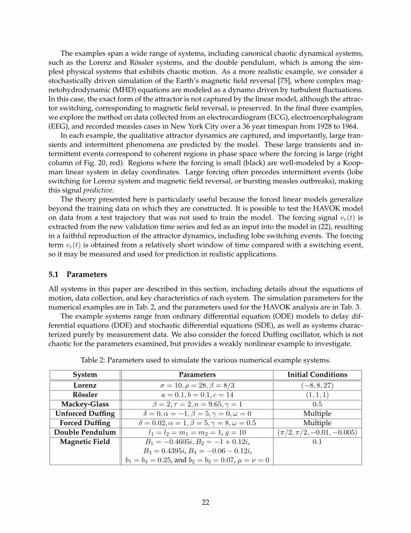
The examples span a wide range of systems, including canonical chaotic dynamical systems,such as the Lorenz and Rossler systems, and the double pendulum, which is among the sim-plest physical systems that exhibits chaotic motion. As a more realistic example, we consider astochastically driven simulation of the Earth’s magnetic field reversal [75], where complex mag-netohydrodynamic (MHD) equations are modeled as a dynamo driven by turbulent fluctuations.In this case, the exact form of the attractor is not captured by the linear model, although the attrac-tor switching, corresponding to magnetic field reversal, is preserved. In the final three examples,we explore the method on data collected from an electrocardiogram (ECG), electroencephalogram(EEG), and recorded measles cases in New York City over a 36 year timespan from 1928 to 1964.

In each example, the qualitative attractor dynamics are captured, and importantly, large tran-sients and intermittent phenomena are predicted by the model. These large transients and in-termittent events correspond to coherent regions in phase space where the forcing is large (rightcolumn of Fig. 20, red). Regions where the forcing is small (black) are well-modeled by a Koop-man linear system in delay coordinates. Large forcing often precedes intermittent events (lobeswitching for Lorenz system and magnetic field reversal, or bursting measles outbreaks), makingthis signal predictive.

The theory presented here is particularly useful because the forced linear models generalizebeyond the training data on which they are constructed. It is possible to test the HAVOK modelon data from a test trajectory that was not used to train the model. The forcing signal vr(t) isextracted from the new validation time series and fed as an input into the model in (22), resultingin a faithful reproduction of the attractor dynamics, including lobe switching events. The forcingterm vr(t) is obtained from a relatively short window of time compared with a switching event,so it may be measured and used for prediction in realistic applications.

5.1 Parameters

All systems in this paper are described in this section, including details about the equations ofmotion, data collection, and key characteristics of each system. The simulation parameters for thenumerical examples are in Tab. 2, and the parameters used for the HAVOK analysis are in Tab. 3.

The example systems range from ordinary differential equation (ODE) models to delay dif-ferential equations (DDE) and stochastic differential equations (SDE), as well as systems charac-terized purely by measurement data. We also consider the forced Duffing oscillator, which is notchaotic for the parameters examined, but provides a weakly nonlinear example to investigate.

Table 2: Parameters used to simulate the various numerical example systems.

System Parameters Initial ConditionsLorenz σ = 10, ρ = 28, β = 8/3 (−8, 8, 27)

Rossler a = 0.1, b = 0.1, c = 14 (1, 1, 1)

Mackey-Glass β = 2, τ = 2, n = 9.65, γ = 1 0.5

Unforced Duffing δ = 0, α = −1, β = 5, γ = 0, ω = 0 MultipleForced Duffing δ = 0.02, α = 1, β = 5, γ = 8, ω = 0.5 Multiple

Double Pendulum l1 = l2 = m1 = m2 = 1, g = 10 (π/2, π/2,−0.01,−0.005)

Magnetic Field B1 = −0.4605i, B2 = −1 + 0.12i, 0.1B3 = 0.4395i, B4 = −0.06− 0.12i,

b1 = b4 = 0.25, and b2 = b3 = 0.07, µ = ν = 0

22

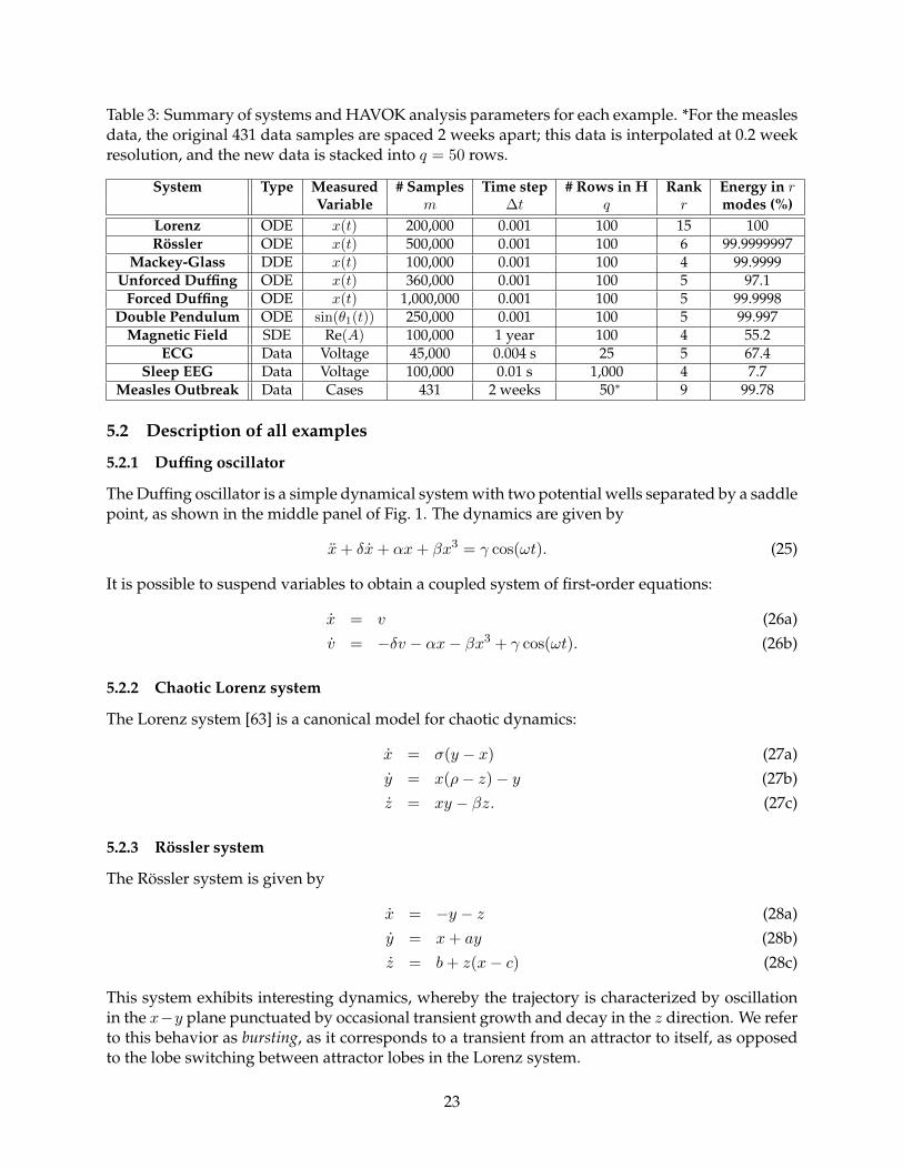
Table 3: Summary of systems and HAVOK analysis parameters for each example. *For the measlesdata, the original 431 data samples are spaced 2 weeks apart; this data is interpolated at 0.2 weekresolution, and the new data is stacked into q = 50 rows.

System Type Measured # Samples Time step # Rows in H Rank Energy in rVariable m ∆t q r modes (%)

Lorenz ODE x(t) 200,000 0.001 100 15 100Rossler ODE x(t) 500,000 0.001 100 6 99.9999997

Mackey-Glass DDE x(t) 100,000 0.001 100 4 99.9999Unforced Duffing ODE x(t) 360,000 0.001 100 5 97.1

Forced Duffing ODE x(t) 1,000,000 0.001 100 5 99.9998Double Pendulum ODE sin(θ1(t)) 250,000 0.001 100 5 99.997

Magnetic Field SDE Re(A) 100,000 1 year 100 4 55.2ECG Data Voltage 45,000 0.004 s 25 5 67.4

Sleep EEG Data Voltage 100,000 0.01 s 1,000 4 7.7Measles Outbreak Data Cases 431 2 weeks 50∗ 9 99.78

5.2 Description of all examples

5.2.1 Duffing oscillator

The Duffing oscillator is a simple dynamical system with two potential wells separated by a saddlepoint, as shown in the middle panel of Fig. 1. The dynamics are given by

x+ δx+ αx+ βx3 = γ cos(ωt). (25)

It is possible to suspend variables to obtain a coupled system of first-order equations:

x = v (26a)v = −δv − αx− βx3 + γ cos(ωt). (26b)

5.2.2 Chaotic Lorenz system

The Lorenz system [63] is a canonical model for chaotic dynamics:

x = σ(y − x) (27a)y = x(ρ− z)− y (27b)z = xy − βz. (27c)

5.2.3 Rossler system

The Rossler system is given by

x = −y − z (28a)y = x+ ay (28b)z = b+ z(x− c) (28c)

This system exhibits interesting dynamics, whereby the trajectory is characterized by oscillationin the x−y plane punctuated by occasional transient growth and decay in the z direction. We referto this behavior as bursting, as it corresponds to a transient from an attractor to itself, as opposedto the lobe switching between attractor lobes in the Lorenz system.

23

5.2.4 Mackey-Glass delay differential equation

The Mackey-Glass equation is a canonical example of a delay differential equation, given by

x(t) = βx(t− τ)

1 + x(t− τ)n− γx(t), (29)

with β = 2, τ = 2, n = 9.65, and γ = 1. The current time dynamics depend on the state x(t− τ) ata previous time τ in the past.

5.2.5 Double pendulum

The double pendulum is among the simplest physical systems that exhibits chaos. The numericalsimulation of the double pendulum is sensitive, and we implement a variational integrator basedon the Euler-Lagrange equations

d

dt

∂L

∂q− ∂L

∂q= 0 (30)

where the Lagrangian L = T − V is the kinetic (T ) minus potential (V ) energy. For the doublependulum, q =

[θ1 θ2

]T , and the Lagrangian becomes:

L = T − V =1

2(m1 +m2)l1θ

21 +

1

2m2l

22θ

22 +m2l1l2θ1θ2 cos(θ1 − θ2)

− (m1 +m2)l1g(1− cos(θ1))−m2l2g (1− cos(θ2)) .

We integrate the equations of motion with a variational integrator derived using a trapezoidalapproximation to the action integral:

δ

∫ b

aL(q, q, t)dt = 0.

Because the mean of θ1 drifts after a revolution, we use x(t) = cos(2θ1(t)) as a measurement.

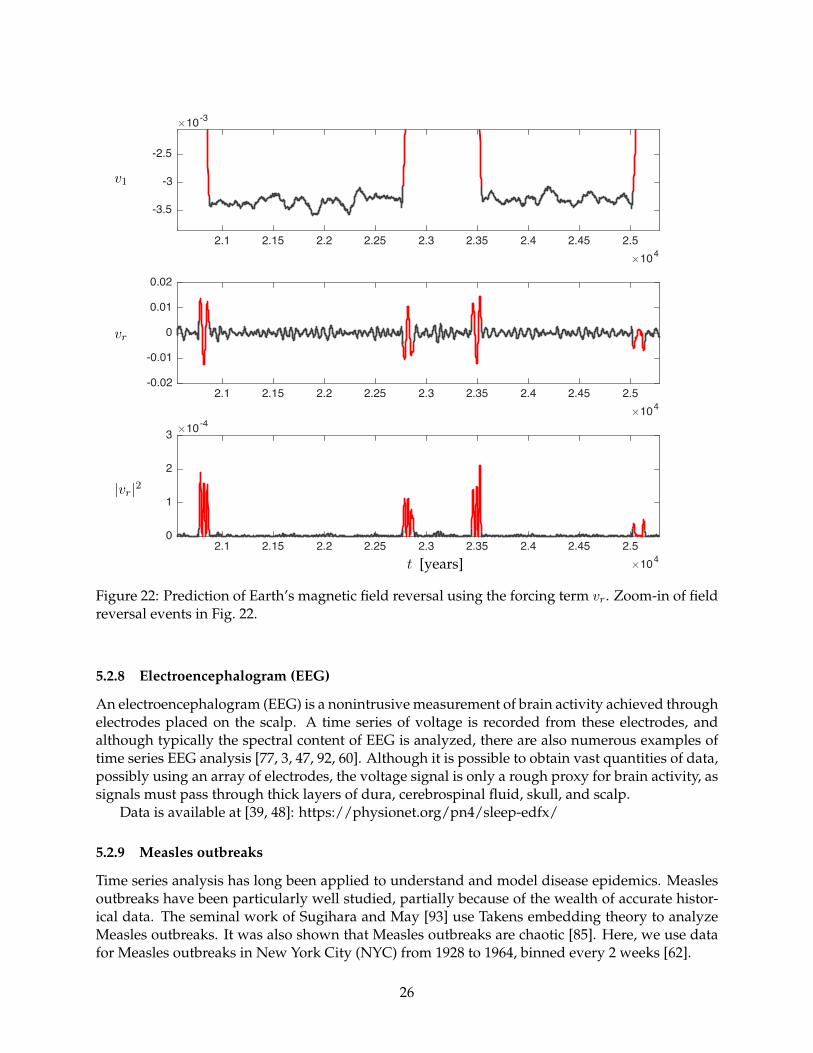
5.2.6 Earth’s magnetic field reversal

The Earth’s magnetic field is known to reverse over geological time scales [23, 41]. Understandingand predicting these rare events is an important challenge in modern geophysics. It is possible tomodel the underlying dynamics that give rise to magnetic field switching by considering the tur-bulent magnetohydrodynamics inside the Earth. A simplified model [73, 75, 74] may be obtainedby modeling the turbulent fluctuations as stochastic forcing on a dynamo.

This is modeled by the following differential equation in terms of the magnetic field A:

d

dtA = µA+ νA+B1A

3 +B2A2A+B3AA

2 +B4A3 + f (31)

where A is the complex conjugate of A and the stochastic forcing f is given by

f = (b1ξ1 + ib3ξ3) Re(A) + (b2ξ2 + ib4ξ4) Im(A).

The variables ξ are Gaussian random variables with a standard deviation of 5. The other parame-ters are given by µ = 1, ν = 0, B1 = −0.4605i, B2 = −1 + 0.12i, B3 = 0.4395i, B4 = −0.06− 0.12i,b1 = b4 = 0.25, and b2 = b3 = 0.07.

24

1 1.2 1.4 1.6 1.8 2 2.2 2.4 2.6×104

-4

-2

0

2

4 ×10-3

1 1.2 1.4 1.6 1.8 2 2.2 2.4 2.6×104

-0.02

-0.01

0

0.01

0.02

1 1.2 1.4 1.6 1.8 2 2.2 2.4 2.6×104

0

1

2

3 ×10-4

Forcing ActiveForcing Inactive

t [years]

|vr|2

vr

v1

Figure 21: Prediction of Earth’s magnetic field reversal using the forcing term vr.

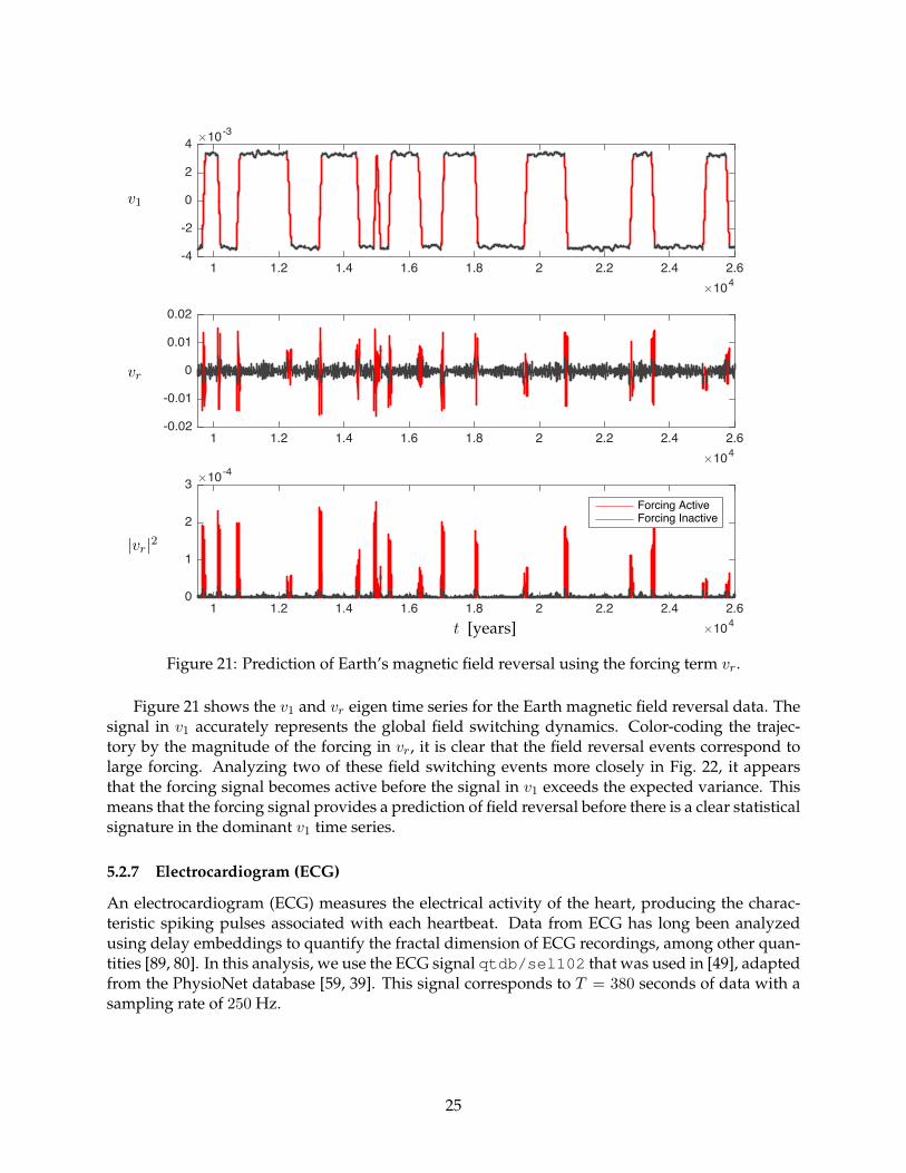
Figure 21 shows the v1 and vr eigen time series for the Earth magnetic field reversal data. Thesignal in v1 accurately represents the global field switching dynamics. Color-coding the trajec-tory by the magnitude of the forcing in vr, it is clear that the field reversal events correspond tolarge forcing. Analyzing two of these field switching events more closely in Fig. 22, it appearsthat the forcing signal becomes active before the signal in v1 exceeds the expected variance. Thismeans that the forcing signal provides a prediction of field reversal before there is a clear statisticalsignature in the dominant v1 time series.

5.2.7 Electrocardiogram (ECG)

An electrocardiogram (ECG) measures the electrical activity of the heart, producing the charac-teristic spiking pulses associated with each heartbeat. Data from ECG has long been analyzedusing delay embeddings to quantify the fractal dimension of ECG recordings, among other quan-tities [89, 80]. In this analysis, we use the ECG signal qtdb/sel102 that was used in [49], adaptedfrom the PhysioNet database [59, 39]. This signal corresponds to T = 380 seconds of data with asampling rate of 250 Hz.

25

2.1 2.15 2.2 2.25 2.3 2.35 2.4 2.45 2.5×104

-3.5

-3

-2.5

×10-3

2.1 2.15 2.2 2.25 2.3 2.35 2.4 2.45 2.5×104

-0.02

-0.01

0

0.01

0.02

2.1 2.15 2.2 2.25 2.3 2.35 2.4 2.45 2.5×104

0

1

2

3 ×10-4

t [years]

|vr|2

vr

v1

Figure 22: Prediction of Earth’s magnetic field reversal using the forcing term vr. Zoom-in of fieldreversal events in Fig. 22.

5.2.8 Electroencephalogram (EEG)

An electroencephalogram (EEG) is a nonintrusive measurement of brain activity achieved throughelectrodes placed on the scalp. A time series of voltage is recorded from these electrodes, andalthough typically the spectral content of EEG is analyzed, there are also numerous examples oftime series EEG analysis [77, 3, 47, 92, 60]. Although it is possible to obtain vast quantities of data,possibly using an array of electrodes, the voltage signal is only a rough proxy for brain activity, assignals must pass through thick layers of dura, cerebrospinal fluid, skull, and scalp.

Data is available at [39, 48]: https://physionet.org/pn4/sleep-edfx/

5.2.9 Measles outbreaks

Time series analysis has long been applied to understand and model disease epidemics. Measlesoutbreaks have been particularly well studied, partially because of the wealth of accurate histor-ical data. The seminal work of Sugihara and May [93] use Takens embedding theory to analyzeMeasles outbreaks. It was also shown that Measles outbreaks are chaotic [85]. Here, we use datafor Measles outbreaks in New York City (NYC) from 1928 to 1964, binned every 2 weeks [62].

26

Figure 23 shows the v1 and vr eigen time series for the Measles outbreaks data. The v1 signalprovides a signature for the severity of the outbreak, with larger negative values correspondingto more cases of Measles. The forcing signal accurately captures many of the outbreaks, mostnotably the largest outbreak after 1940. This outbreak was preceded by two small dips in v1,which may have resulted in false positives using other prediction methods. However, the forcingsignal becomes large directly preceding the outbreak.

1930 1940 1950 1960-0.1

-0.05

0

1930 1940 1950 1960-0.2

-0.1

0

0.1

0.2

1930 1940 1950 19600

0.005

0.01

0.015

0.02Forcing ActiveForcing Inactive

t

|vr|2

vr

v1

Figure 23: Prediction of Measles outbreaks using the forcing term vr.

6 Discussion

In summary, we have presented a data-driven procedure, the HAVOK analysis, to identify anintermittently forced linear system representation of chaos. This procedure is based on machinelearning regressions, Takens’ embedding, and Koopman operator theory. The activity of the forc-ing signal in these models predicts intermittent transient events, such as lobe switching and burst-ing, and partitions phase space into coherent linear and nonlinear regions. More generally, thesearch for intrinsic or natural measurement coordinates is of central importance in finding sim-ple representations of complex systems, and this will only become increasingly important withgrowing data. Simple, linear representations of complex systems is a long sought goal, providingthe hope for a general theory of nonlinear estimation, prediction, and control. This analysis willhopefully motivate novel strategies to measure, understand, and control [90] chaotic systems in avariety of scientific and engineering applications.

27

References

[1] H. D. I. Abarbanel, R. Brown, J. J. Sidorowich, and L. S. Tsimring. The analysis of observedchaotic data in physical systems. Reviews of Modern Physics, 65(4):1331, 1993.

[2] R. Abraham, J. E. Marsden, and T. Ratiu. Manifolds, Tensor Analysis, and Applications, vol-ume 75 of Applied Mathematical Sciences. Springer-Verlag, 1988.

[3] R. Acharya, O. Faust, N. Kannathal, T. Chua, and S. Laxminarayan. Non-linear analysis ofEEG signals at various sleep stages. Computer methods and programs in biomedicine, 80(1):37–45, 2005.

[4] D. Aeyels. Generic observability of differentiable systems. SIAM Journal on Control andOptimization, 19(5):595–603, 1981.

[5] L. A. Aguirre and C. Letellier. Observability of multivariate differential embeddings. Journalof Physics A: Mathematical and General, 38(28):6311, 2005.

[6] H. Babaee and T. P. Sapsis. A minimization principle for the description of modes associatedwith finite-time instabilities. Proc. R. Soc. A, 472(2186), 2016.

[7] S. Bagheri. Koopman-mode decomposition of the cylinder wake. Journal of Fluid Mechanics,726:596–623, 2013.

[8] Z. Bai, T. Wimalajeewa, Z. Berger, G. Wang, M. Glauser, and P. K. Varshney. Low-dimensional approach for reconstruction of airfoil data via compressive sensing. AIAAJournal, pages 1–14, 2014.

[9] O. N. Bjørnstad and B. T. Grenfell. Noisy clockwork: time series analysis of populationfluctuations in animals. Science, 293(5530):638–643, 2001.

[10] J. Bongard and H. Lipson. Automated reverse engineering of nonlinear dynamical systems.Proceedings of the National Academy of Sciences, 104(24):9943–9948, 2007.

[11] D. S. Broomhead and R. Jones. Time-series analysis. Proc. Roy. Soc. A, 423(1864):103–121,1989.

[12] S. L. Brunton and B. R. Noack. Closed-loop turbulence control: Progress and challenges.Applied Mechanics Reviews, 67:050801–1–050801–48, 2015.

[13] S. L. Brunton, J. L. Proctor, and J. N. Kutz. Discovering governing equations from data bysparse identification of nonlinear dynamical systems. PNAS, 113(15):3932–3937, 2016.

[14] S. L. Brunton, J. H. Tu, I. Bright, and J. N. Kutz. Compressive sensing and low-rank librariesfor classification of bifurcation regimes in nonlinear dynamical systems. SIAM Journal onApplied Dynamical Systems, 13(4):1716–1732, 2014.

[15] S. L. Brunton, B. W. Brunton, J. L. Proctor, and J.N. Kutz. Koopman observable subspacesand finite linear representations of nonlinear dynamical systems for control. PLoS ONE,11(2):e0150171, 2016.

[16] M. Budisic and I. Mezic. An approximate parametrization of the ergodic partition usingtime averaged observables. 48th IEEE Conf. on Decision and Control, pages 3162–3168, 2009.

28

[17] M. Budisic and I. Mezic. Geometry of the ergodic quotient reveals coherent structures inflows. Physica D, 241(15):1255–1269, 2012.

[18] M. Budisic, R. Mohr, and I. Mezic. Applied Koopmanism a). Chaos: An InterdisciplinaryJournal of Nonlinear Science, 22(4):047510, 2012.

[19] K. K. Chen, J. H. Tu, and C. W. Rowley. Variants of dynamic mode decomposition: Boundarycondition, Koopman, and Fourier analyses. Journal of Nonlinear Science, 22(6):887–915, 2012.

[20] A. J. Chorin and J. E. Marsden. A mathematical introduction to fluid mechanics, volume 3.Springer, 1990.

[21] W. Cousins and T. P. Sapsis. Quantification and prediction of extreme events in a one-dimensional nonlinear dispersive wave model. Physica D, 280:48–58, 2014.

[22] W. Cousins and T. P. Sapsis. Reduced-order precursors of rare events in unidirectional non-linear water waves. Journal of Fluid Mechanics, 790:368–388, 2016.

[23] A. Cox, R. R. Doell, and G. B. Dalrymple. Reversals of the Earth’s magnetic field. Science,144(3626):1537–1543, 1964.

[24] J. P. Crutchfield. Between order and chaos. Nature Physics, 8(1):17–24, 2012.

[25] J. P. Crutchfield and B. S. McNamara. Equations of motion from a data series. ComplexSystems, 1:417–452, 1987.

[26] M. Dellnitz, G. Froyland, and O. Junge. The algorithms behind GAIO—set oriented nu-merical methods for dynamical systems. In Ergodic theory, analysis, and efficient simulation ofdynamical systems, pages 145–174. Springer, 2001.

[27] M. Dellnitz and O. Junge. Set oriented numerical methods for dynamical systems. Handbookof dynamical systems, 2:221–264, 2002.

[28] M. Dellnitz, O. Junge, W. S. Koon, F. Lekien, M. W. Lo, J. E. Marsden, K. Padberg, R. Preis,S. D. Ross, and B. Thiere. Transport in dynamical astronomy and multibody problems.International Journal of Bifurcation and Chaos, 15:699–727, 2005.

[29] G. E. Dullerud and F. Paganini. A course in robust control theory: A convex approach. Texts inApplied Mathematics. Springer, Berlin, Heidelberg, 2000.

[30] J. D. Farmer and J. J. Sidorowich. Predicting chaotic time series. Physical Review Letters,59(8):845, 1987.

[31] G. Froyland, G. A. Gottwald, and A. Hammerlindl. A computational method to extractmacroscopic variables and their dynamics in multiscale systems. SIAM Journal on AppliedDynamical Systems, 13(4):1816–1846, 2014.

[32] G. Froyland and K. Padberg. Almost-invariant sets and invariant manifolds – connectingprobabilistic and geometric descriptions of coherent structures in flows. Physica D, 238:1507–1523, 2009.

[33] G. Froyland, N. Santitissadeekorn, and A. Monahan. Transport in time-dependent dynami-cal systems: Finite-time coherent sets. Chaos, 20(4):043116–1–043116–16, 2010.

29

[34] Gary Froyland. Statistically optimal almost-invariant sets. Physica D, 200(3):205–219, 2005.

[35] P. Gaspard, G. Nicolis, and A. Provata. Spectral signature of the pitchfork bifurcation: Liou-ville equation approach. Physical Review E, 51(1):74–94, 1995.

[36] M. Gavish and D. L. Donoho. The optimal hard threshold for singular values is 4/√

3. IEEETransactions on Information Theory, 60(8):5040–5053, 2014.

[37] D. Giannakis. Data-driven spectral decomposition and forecasting of ergodic dynamicalsystems. arXiv preprint arXiv:1507.02338, 2015.

[38] D. Giannakis and A. J. Majda. Nonlinear Laplacian spectral analysis for time series withintermittency and low-frequency variability. PNAS, 109(7):2222–2227, 2012.

[39] A. L Goldberger, L. A. N. Amaral, L. Glass, J. M. Hausdorff, P.-Ch. Ivanov, R. G. Mark, J. E.Mietus, G. B. Moody, C.-K. Peng, and H. E. Stanley. Physiobank, physiotoolkit, and phys-ionet components of a new research resource for complex physiologic signals. Circulation,101(23):e215–e220, 2000.

[40] J. Guckenheimer and P. Holmes. Nonlinear oscillations, dynamical systems, and bifurcations ofvector fields, volume 42 of Applied Mathematical Sciences. Springer, 1983.

[41] Y. Guyodo and J.-P. Valet. Global changes in intensity of the Earth’s magnetic field duringthe past 800 kyr. Nature, 399(6733):249–252, 1999.

[42] R. Hermann and A. J. Krener. Nonlinear controllability and observability. IEEE Transactionson automatic control, 22(5):728–740, 1977.

[43] B. L. Ho and R. E. Kalman. Effective construction of linear state-variable models from in-put/output data. In Proc. 3rd AAC, pages 449–459, 1965.

[44] J. N. Juang and R. S. Pappa. An eigensystem realization algorithm for modal parameteridentification and model reduction. J. of Guidance, Control, and Dynamics, 8(5):620–627, 1985.

[45] E. Kaiser, B. R. Noack, L. Cordier, A. Spohn, M. Segond, M. Abel, G. Daviller, J. Osth, S. Kra-jnovic, and R. K. Niven. Cluster-based reduced-order modelling of a mixing layer. J. FluidMech., 754:365–414, 2014.

[46] R. E. Kalman. A new approach to linear filtering and prediction problems. Journal of FluidsEngineering, 82(1):35–45, 1960.

[47] N. Kannathal, M. L. Choo, U. R. Acharya, and P. K. Sadasivan. Entropies for detection ofepilepsy in EEG. Computer methods and programs in biomedicine, 80(3):187–194, 2005.

[48] Bob Kemp, Aeilko H Zwinderman, Bert Tuk, Hilbert AC Kamphuisen, and Josefien JLOberye. Analysis of a sleep-dependent neuronal feedback loop: the slow-wave microconti-nuity of the eeg. IEEE Transactions on Biomedical Engineering, 47(9):1185–1194, 2000.

[49] E. Keogh, J. Lin, and A. Fu. HOT SAX: Efficiently finding the most unusual time seriessubsequence. In Fifth IEEE International Conference on Data Mining, 2005.

[50] I. G. Kevrekidis, C. W. Gear, J. M. Hyman, P. G. Kevrekidis, O. Runborg, and C. Theodor-opoulos. Equation-free, coarse-grained multiscale computation: Enabling microscopic sim-ulators to perform system-level analysis. Communications in Mathematical Science, 1(4):715–762, 2003.

30

[51] A.N. Kolmogorov. Dissipation of energy in locally isotropic turbulence. Dokl. Akad. NaukSSSR, 32:16–18, 1941. (translated and reprinted 1991 in Proceedings of the Royal Society A434, 15–17).

[52] A.N. Kolmogorov. The local structure of turbulence in incompressible viscous fluid for verylarge Reynolds number. Dokl. Akad. Nauk SSSR, 30:9–13, 1941. (translated and reprinted1991 in Proceedings of the Royal Society A 434, 9–13).

[53] A.N. Kolmogorov. On degeneration (decay) of isotropic turbulence. Dokl. Akad. Nauk SSSR,31:538–540, 1941.

[54] W. S. Koon, M. W. Lo, J. E. Marsden, and S. D. Ross. Heteroclinic connections betweenperiodic orbits and resonance transitions in celestial mechanics. Chaos: An InterdisciplinaryJournal of Nonlinear Science, 10(2):427–469, 2000.

[55] B. O. Koopman. Hamiltonian systems and transformation in Hilbert space. PNAS, 17(5):315–318, 1931.

[56] B. O. Koopman and J.-v. Neumann. Dynamical systems of continuous spectra. Proceedingsof the National Academy of Sciences of the United States of America, 18(3):255, 1932.

[57] J. R. Koza, F. H. Bennett III, and O. Stiffelman. Genetic programming as a Darwinian inven-tion machine. In Genetic Programming, pages 93–108. Springer, 1999.

[58] J. N. Kutz, S. L. Brunton, B. W. Brunton, and J. L. Proctor. Dynamic Mode Decomposition:Data-Driven Modeling of Complex Systems. SIAM, 2016.

[59] P. Laguna, R. G. Mark, A. Goldberg, and G. B. Moody. A database for evaluation of al-gorithms for measurement of qt and other waveform intervals in the ecg. In Computers inCardiology 1997, pages 673–676. IEEE, 1997.

[60] Claudia Lainscsek, Manuel E Hernandez, Howard Poizner, and Terrence J Sejnowski. Delaydifferential analysis of electroencephalographic data. Neural computation, 2015.

[61] Y. Lan and I. Mezic. Linearization in the large of nonlinear systems and Koopman operatorspectrum. Physica D, 242(1):42–53, 2013.

[62] W. P. London and J. A. Yorke. Recurrent outbreaks of measles, chickenpox and mumps i.seasonal variation in contact rates. American journal of epidemiology, 98(6):453–468, 1973.

[63] E. N. Lorenz. Deterministic nonperiodic flow. Journal of Atmospheric Sciences, 20(2):130–141,1963.

[64] A. Mackey, H. Schaeffer, and S. Osher. On the compressive spectral method. MultiscaleModeling & Simulation, 12(4):1800–1827, 2014.

[65] A. J. Majda and J. Harlim. Information flow between subspaces of complex dynamical sys-tems. PNAS, 104(23):9558–9563, 2007.

[66] A. J. Majda and J. Harlim. Physics constrained nonlinear regression models for time series.Nonlinearity, 26(1):201, 2012.

[67] A. J. Majda and Y. Lee. Conceptual dynamical models for turbulence. PNAS, 111(18):6548–6553, 2014.

31

[68] J. E. Marsden and M. McCracken. The Hopf bifurcation and its applications, volume 19.Springer-Verlag, 1976.

[69] J. E. Marsden and T. S. Ratiu. Introduction to mechanics and symmetry. Springer-Verlag, 2ndedition, 1999.

[70] I. Mezic. Spectral properties of dynamical systems, model reduction and decompositions.Nonlinear Dynamics, 41(1-3):309–325, 2005.

[71] I. Mezic. Analysis of fluid flows via spectral properties of the Koopman operator. AnnualReview of Fluid Mechanics, 45:357–378, 2013.

[72] V. Ozolins, R. Lai, R. Caflisch, and S. Osher. Compressed modes for variational problemsin mathematics and physics. Proceedings of the National Academy of Sciences, 110(46):18368–18373, 2013.

[73] F. Petrelis and S. Fauve. Chaotic dynamics of the magnetic field generated by dynamo actionin a turbulent flow. Journal of Physics: Condensed Matter, 20(49):494203, 2008.

[74] F. Petrelis and S. Fauve. Mechanisms for magnetic field reversals. Philosophical Transactions ofthe Royal Society of London A: Mathematical, Physical and Engineering Sciences, 368(1916):1595–1605, 2010.

[75] F. Petrelis, S. Fauve, E. Dormy, and J.-P. Valet. Simple mechanism for reversals of Earth’smagnetic field. Physical Review Letters, 102(14):144503, 2009.

[76] H. Poincare. Sur le probleme des trois corps et les equations de la dynamique. Acta Mathe-matica, 13(1):A3–A270, 1890.

[77] W. S. Pritchard and D. W. Duke. Measuring chaos in the brain: a tutorial review of nonlineardynamical EEG analysis. International Journal of Neuroscience, 67(1-4):31–80, 1992.

[78] J. L. Proctor, S. L. Brunton, B. W. Brunton, and J. N. Kutz. Exploiting sparsity and equation-free architectures in complex systems (invited review). The European Physical Journal SpecialTopics, 223(13):2665–2684, 2014.

[79] J. L. Proctor, S. L. Brunton, and J. N. Kutz. Dynamic mode decomposition with control.SIAM Journal on Applied Dynamical Systems, 15(1):142–161, 2016.

[80] M. Richter and T. Schreiber. Phase space embedding of electrocardiograms. Physical ReviewE, 58(5):6392, 1998.

[81] G. Rowlands and J. C. Sprott. Extraction of dynamical equations from chaotic data. PhysicaD, 58(1-4):251–259, 1992.

[82] C. W. Rowley, I. Mezic, S. Bagheri, P. Schlatter, and D.S. Henningson. Spectral analysis ofnonlinear flows. Journal of Fluid Mechanics, 645:115–127, 2009.

[83] T. P. Sapsis and A. J. Majda. Statistically accurate low-order models for uncertainty quantifi-cation in turbulent dynamical systems. PNAS, 110(34):13705–13710, 2013.

[84] H. Schaeffer, R. Caflisch, C. D. Hauck, and S. Osher. Sparse dynamics for partial differentialequations. Proceedings of the National Academy of Sciences USA, 110(17):6634–6639, 2013.

32

[85] W. M. Schaffer and M. Kot. Do strange attractors govern ecological systems? BioScience,35(6):342–350, 1985.

[86] P. J. Schmid. Dynamic mode decomposition of numerical and experimental data. Journal ofFluid Mechanics, 656:5–28, August 2010.

[87] P. J. Schmid and J. Sesterhenn. Dynamic mode decomposition of numerical and experimen-tal data. In 61st Annual Meeting of the APS Division of Fluid Dynamics. American PhysicalSociety, November 2008.

[88] M. Schmidt and H. Lipson. Distilling free-form natural laws from experimental data. Science,324(5923):81–85, 2009.

[89] T. Schreiber and D. T. Kaplan. Nonlinear noise reduction for electrocardiograms. Chaos: AnInterdisciplinary Journal of Nonlinear Science, 6(1):87–92, 1996.

[90] T. Shinbrot, C. Grebogi, E. Ott, and J. A. Yorke. Using small perturbations to control chaos.Nature, 363(6428):411–417, 1993.

[91] S. Skogestad and I. Postlethwaite. Multivariable feedback control: analysis and design. JohnWiley & Sons, Inc., Hoboken, New Jersey, 2 edition, 2005.

[92] C. J. Stam. Nonlinear dynamical analysis of EEG and MEG: review of an emerging field.Clinical Neurophysiology, 116(10):2266–2301, 2005.

[93] G. Sugihara and R. M. May. Nonlinear forecasting as a way of distinguishing chaos frommeasurement error in time series. Nature, 344(6268):734–741, 1990.

[94] G. Sugihara, R. M. May, H. Ye, C.-H. Hsieh, E. Deyle, M. Fogarty, and S. Munch. Detectingcausality in complex ecosystems. Science, 338(6106):496–500, 2012.

[95] F. Takens. Detecting strange attractors in turbulence. Lecture Notes in Mathematics, 898:366–381, 1981.

[96] R. Tibshirani. Regression shrinkage and selection via the lasso. J. of the Royal StatisticalSociety B, pages 267–288, 1996.

[97] A. A. Tsonis and J. B. Elsner. Nonlinear prediction as a way of distinguishing chaos fromrandom fractal sequences. Nature, 1992.

[98] J. H. Tu, C. W. Rowley, D. M. Luchtenburg, S. L. Brunton, and J. N. Kutz. On dynamic modedecomposition: theory and applications. J. of Computational Dynamics, 1(2):391–421, 2014.

[99] W. X. Wang, R. Yang, Y. C. Lai, V. Kovanis, and C. Grebogi. Predicting catastrophes innonlinear dynamical systems by compressive sensing. PRL, 106:154101, 2011.

[100] G. Welch and G. Bishop. An introduction to the Kalman filter, 1995.

[101] M. O. Williams, I. G. Kevrekidis, and C. W. Rowley. A data-driven approximation of theKoopman operator: extending dynamic mode decomposition. J. Nonlin. Science, 2015.

[102] H. Ye, R. J. Beamish, S. M. Glaser, S. C. H. Grant, C.-H. Hsieh, L. J. Richards, J. T. Schnute,and G. Sugihara. Equation-free mechanistic ecosystem forecasting using empirical dynamicmodeling. PNAS, 112(13):E1569–E1576, 2015.

33

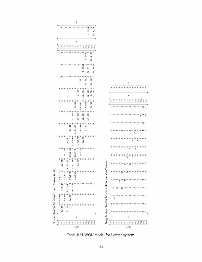
0 -

5.09

84

0

-0.1

175

0

0

0

0

0

0

0

0

0

0

5.10

56

0 -

9.93

91

0

-0.

1875

0

0

0

0

0

0

0

0

0

0

9.90

68

0 -

13.5

674

0

0.

2450

0

0

0

0

0

0

0

0

0.10

28

0 1

3.50

45

0

-18.

9515

0

0

.333

7

0

0

0

0

0

0

0

0

0.13

97

0

18.8

743

0

23.

2686

0

0.41

05

0

0

0

0

0

0

0

0 -

0.18

95

0

-23.

1969

0

-28

.999

6

0

-0.5

105

0

0

0

0

0

0

0

0

-0.2

984

0

28.

9711

0 -3

3.57

79

0

0.5

945

0

0

0

0

0

0

0

0

-0.

3999

0

33

.575

9

0 -

39.4

090

0

0.

7005

0

0

0

0

0

0

0

0

0.

5710

0 3

9.41

66

0

44.0

851

0

0

.787

5

0

0

0

0

0

0

0

0

-0

.626

1

0 -

44.0

173

0

-50.

0746

0

0.89

81

0

0

0

0

0

0

0

0 -

0.71

73

0

49.9

095

0

-54

.652

9

0

0.9

830

0

0

0

0

0

0

0

0

-0.6

723

0

54.

3722

0 6

0.83

19

0

0

0

0

0

0

0

0

0

0

-0.7

197

0.

2934

-60

.528

7

0 -

65.1

484

0

0

0

0

0

0

0

0

0

0

-0.

7977

0 6

4.94

82

0

2 6 6 6 6 6 6 6 6 6 6 6 6 6 6 6 6 6 6 6 6 6 6 4

0 5 10 15 20 25 30 35 40 45 50 55 60 65

3 7 7 7 7 7 7 7 7 7 7 7 7 7 7 7 7 7 7 7 7 7 7 5

2 6 6 6 6 6 6 6 6 6 6 6 6 6 6 6 6 6 6 6 6 6 6 4

0 5 10 15 20 25 30 35 40 45 50 55 60 65

3 7 7 7 7 7 7 7 7 7 7 7 7 7 7 7 7 7 7 7 7 7 7 5

0

0

0

0

0

0

0

0

0

0

0

1.

0964

0

-71.

5168

2 6 6 6 6 6 6 6 6 6 6 6 6 6 6 6 6 6 6 6 6 6 6 4

0 5 10 15 20 25 30 35 40 45 50 55 60 65

3 7 7 7 7 7 7 7 7 7 7 7 7 7 7 7 7 7 7 7 7 7 7 5

2 6 6 6 6 6 6 6 6 6 6 6 6 6 6 6 6 6 6 6 6 6 6 4

0 5 10 15 20 25 30 35 40 45 50 55 60 65

3 7 7 7 7 7 7 7 7 7 7 7 7 7 7 7 7 7 7 7 7 7 7 5

d dt

2 6 6 6 6 6 6 6 6 6 6 6 6 6 6 6 6 6 6 6 6 6 6 4

v 1 v 2 v 3 v 4 v 5 v 6 v 7 v 8 v 9 v 10

v 11

v 12

v 13

v 14

3 7 7 7 7 7 7 7 7 7 7 7 7 7 7 7 7 7 7 7 7 7 7 5

v 15

=

2 6 6 6 6 6 6 6 6 6 6 6 6 6 6 6 6 6 6 6 6 6 6 4

v 1 v 2 v 3 v 4 v 5 v 6 v 7 v 8 v 9 v 10

v 11

v 12

v 13

v 14

3 7 7 7 7 7 7 7 7 7 7 7 7 7 7 7 7 7 7 7 7 7 7 5

+

0

-5

0

0

0

0

0

0

0

0

0

0

0

0

5

0

-

10

0

0

0

0

0

0

0

0

0

0

0

0

10

0

-15

0

0

0

0

0

0

0

0

0

0

0

0

15

0

-

20

0

0

0

0

0

0

0

0

0

0

0

0

20

0

25

0

0

0

0

0

0

0

0

0

0

0

0

-

25

0

-

30

0

0

0

0

0

0

0

0

0

0

0

0

30

0

-35

0

0

0

0

0

0

0

0

0

0

0

0

35

0

-

40

0

0

0

0

0

0

0

0

0

0

0

0

40

0

45

0

0

0

0

0

0

0

0

0

0

0

0

-

45

0

-

50

0

0

0

0

0

0

0

0

0

0

0

0

50

0

-55

0

0

0

0

0

0

0

0

0

0

0

0

55

0

60

0

0

0

0

0

0

0

0

0

0

0

0

-60

0

-65

0

0

0

0

0

0

0

0

0

0

0

0

65

0

2 6 6 6 6 6 6 6 6 6 6 6 6 6 6 6 6 6 6 6 6 6 6 4

0 5 10 15 20 25 30 35 40 45 50 55 60 65

3 7 7 7 7 7 7 7 7 7 7 7 7 7 7 7 7 7 7 7 7 7 7 5

2 6 6 6 6 6 6 6 6 6 6 6 6 6 6 6 6 6 6 6 6 6 6 4

0 5 10 15 20 25 30 35 40 45 50 55 60 65

3 7 7 7 7 7 7 7 7 7 7 7 7 7 7 7 7 7 7 7 7 7 7 5

0

0

0

0

0

0

0

0

0

0

0

0

0

-70

2 6 6 6 6 6 6 6 6 6 6 6 6 6 6 6 6 6 6 6 6 6 6 4

0 5 10 15 20 25 30 35 40 45 50 55 60 65

3 7 7 7 7 7 7 7 7 7 7 7 7 7 7 7 7 7 7 7 7 7 7 5

2 6 6 6 6 6 6 6 6 6 6 6 6 6 6 6 6 6 6 6 6 6 6 4

0 5 10 15 20 25 30 35 40 45 50 55 60 65

3 7 7 7 7 7 7 7 7 7 7 7 7 7 7 7 7 7 7 7 7 7 7 5

2 6 6 6 6 6 6 6 6 6 6 6 6 6 6 6 6 6 6 6 6 6 6 4

v 1 v 2 v 3 v 4 v 5 v 6 v 7 v 8 v 9 v 10

v 11

v 12

v 13

v 14

3 7 7 7 7 7 7 7 7 7 7 7 7 7 7 7 7 7 7 7 7 7 7 5

d dt

2 6 6 6 6 6 6 6 6 6 6 6 6 6 6 6 6 6 6 6 6 6 6 4

v 1 v 2 v 3 v 4 v 5 v 6 v 7 v 8 v 9 v 10

v 11

v 12

v 13

v 14

3 7 7 7 7 7 7 7 7 7 7 7 7 7 7 7 7 7 7 7 7 7 7 5

=+

v 15

Spar

se H

AVO

K M

odel

of L

oren

z Sy

stem

(r=1

4)

Nei

ghbo

ring

HAV

OK

Mod

el w

ith In

tege

r Coe

ffici

ents

Table 4: HAVOK model for Lorenz system.

34