Embed Size (px)
Citation preview

CHAOS 2020
Proceedings
13th Chaotic Modeling and Simulation
International Conference
Editor
Christos H. Skiadas
9-12 June, 2020

ii
Imprint
Proceedings of the 13th Chaotic Modeling and Simulation
International Conference (9-12 June, 2020)
Published by: ISAST: International Society for the Advancement of
Science and Technology.
Editor: Christos H Skiadas
© Copyright 2020 by ISAST: International Society for the Advancement of
Science and Technology.
All rights reserved. No part of this publication may be reproduced, stored,
retrieved or transmitted, in any form or by any means, without the written
permission of the publisher, nor be otherwise circulated in any form of binding
or cover.

iii
Preface 13th Chaotic Modeling and Simulation
International Conference
9 – 12 June 2020
It is our pleasure to welcome the guests, participants and contributors to
the 13th International Conference (CHAOS2020) on Chaotic Modeling,
Simulation and Applications. We support the study of nonlinear systems
and dynamics in an interdisciplinary research field and very interesting
applications will be presented. We intend to provide a widely selected
forum to exchange ideas, methods, and techniques in the field of
Nonlinear Dynamics, Chaos, Fractals and their applications in General
Science and in Engineering Sciences.
The principal aim of CHAOS2020 International Conference is to expand
the development of the theories of the applied nonlinear field, the
methods and the empirical data and computer techniques, and the best
theoretical achievements of chaotic theory as well.
Chaotic Modeling and Simulation Conferences continue to grow
considerably from year to year thus making a well established platform
to present and disseminate new scientific findings and interesting
applications.
We thank all the contributors to the success of this conference and
especially the authors of this Proceedings Volume. Special thanks to the
Plenary, Keynote and Invited Presentations, the Scientific Committee,
the ISAST Committee, Yiannis Dimotikalis and Aris Meletiou and the
web supporting team, the Conference Secretary Eleni Molfesi and all the
members of the Secretariat.
November 2020
Christos H. Skiadas,
Conference Chair

iv

v
Honorary Committee and Scientific Advisors
Florentino Borondo Rodríguez Universidad Autónoma de Madrid,
Instituto de Ciencias Matemáticas, ICMAT (CSIC-UAM-UCM-UCIII)
Leon O. Chua EECS Department, University of California, Berkeley, USA
Honorary Editor of the International Journal of Bifurcation and Chaos
Giovanni Gallavotti Universita di Roma 1, "La Sapienza", Italy and Rutgers University, USA
Gennady A. Leonov (1947-2018) Dean of Mathematics and Mechanics Faculty, Saint-Petersburg State University,
Russia, Member (corresponding) of Russian Academy of Science
Gheorghe Mateescu Department of Chemistry, Case Western Reserve University, Cleveland, OH,
USA
Yves Pomeau Department of Mathematics, University of Arizona, Tucson, USA
David Ruelle Academie des Sciences de Paris, Honorary Professor at the Institut des Hautes
Etudes Scientifiques of Bures-sur-Yvette, France
Ferdinand Verhulst Institute of Mathematics, Utrecht, The Netherlands
International Scientific Committee
C. H. Skiadas (ManLab, Technical University of Crete, Chania, Greece), Co-Chair
H. Adeli (The Ohio State University, USA)
J.-O. Aidanpaa (Division of Solid Mechanics, Lulea University of Technology, Sweden)
N. Akhmediev (Australian National University, Australia)
M. Amabili (McGill University, Montreal, Canada)
J. Awrejcewicz (Technical University of Lodz, Poland)
E. Babatsouli (University of Crete, Rethymnon, Greece)
J. M. Balthazar (UNESP-Rio Claro, State University of Sao Paulo, Brasil)
S. Bishop (University College London, UK)
T. Bountis (Department of Mathematics, Nazarbayev University, Astana, Kazakhstan)
Y. S. Boutalis (Democritus University of Thrace, Greece)
C. Chandre (Centre de Physique Theorique, Marseille, France)
M. Christodoulou (Technical University of Crete, Chania, Crete, Greece)
P. Commendatore (Universita di Napoli 'Federico II', Italy)
D. Dhar (Tata Institute of Fundamental Research, India)
J. Dimotikalis (Technological Educational Institute, Crete, Greece)
B. Epureanu (University of Michigan, Ann Arbor, MI, USA)
G. Fagiolo (Sant'Anna School of Advanced Studies, Pisa, Italy)
M. I. Gomes (Lisbon University and CEAUL, Lisboa, Portugal)
V. Grigoras (University of Iasi, Romania)

vi
A. S. Hacinliyan (Yeditepe University, Istanbul, Turkey)
K. Hagan, (University of Limerick, Ireland)
L. Hong (Xi'an Jiaotong University, Xi'an, Shaanxi, China)
G. Hunt (Centre for Nonlinear Mechanics, University of Bath, Bath, UK)
T. Kapitaniak (Technical University of Lodz, Lodz, Poland)
G. P. Kapoor (Indian Institute of Technology Kanpur, Kanpur, India)
W. Klonowski (Nalecz Institute of Biocybernetics and Biomedical Engineering, Polish Academy of Sciences, Warsaw, Poland)
A. Kolesnikov (Southern Federal University Russia)
I. Kourakis (Khalifa University of Science and Technology, Abu Dhabi, UAE)
J. Kretz (University of Music and Performing Arts, Vienna, Austria)
V. Krysko (Dept. of Math. and Modeling, Saratov State Technical University, Russia)
I. Kusbeyzi Aybar (Yeditepe University, Istanbul, Turkey)
W. Li (Northwestern Polytechnical University, China)
B. L. Lan (School of Engineering, Monash University, Selangor, Malaysia)
V J Law (University College Dublin, Dublin, Ireland)
I. Lubashevsky (The University of Aizu, Japan)
V. Lucarini (University of Hamburg, Germany)
J. A. T. Machado (ISEP-Institute of Engineering of Porto, Porto, Portugal)
W. M. Macek (Cardinal Stefan Wyszynski University, Warsaw, Poland)
P. Mahanti (University of New Brunswick, Saint John, Canada)
G. M. Mahmoud (Assiut University, Assiut, Egypt)
R. Manca (“Sapienza” University of Rome, Italy)
P. Manneville (Laboratoire d'Hydrodynamique, Ecole Polytechnique, France)
A. S. Mikhailov (Fritz Haber Institute of Max Planck Society, Berlin, Germany)
E. R. Miranda (University of Plymouth, UK)
M. S. M. Noorani (University Kebangsaan, Malaysia)
G. V. Orman (Transilvania University of Brasov, Romania)
O. Ozgur Aybar (Dept of Math., Piri Reis University, Tuzla, Istanbul, Turkey)
S. Panchev (Bulgarian Academy of Sciences, Bulgaria)
G. P. Pavlos (Democritus University of Thrace, Greece)
G. Pedrizzetti (University of Trieste, Trieste, Italy)
F. Pellicano (Universita di Modena e Reggio Emilia, Italy)
D. Pestana (Lisbon University and CEAUL, Lisboa, Portugal)
S. V. Prants (Pacific Oceanological Institute of RAS, Vladivostok, Russia)
A.G. Ramm (Kansas State University, Kansas, USA)
G. Rega (University of Rome "La Sapienza", Italy)
H. Skiadas (Hanover College, Hanover, USA)
V. Snasel (VSB-Technical University of Ostrava, Czech)
D. Sotiropoulos (Technical University of Crete, Chania, Crete, Greece)
B. Spagnolo (University of Palermo, Italy)
P. D. Spanos (Rice University, Houston, TX, USA)
J. C. Sprott (University of Wisconsin, Madison, WI, USA)
S. Thurner (Medical University of Vienna, Austria)
D. Trigiante (Universita di Firenze, Firenze, Italy)
G. Unal (Yeditepe University, Istanbul, Turkey)
A. Valyaev (Nuclear Safety Institute of RAS, Russia)
A. Vakakis (University of Illinois at Urbana-Champaign, Illinois, USA)
J. P. van der Weele (University of Patras, Greece)
M. Wiercigroch (University of Aberdeen, Aberdeen, Scotland, UK)
M. V. Zakrzhevsky (Institute of Mechanics, Riga Technical University, Latvia)
J. Zhang (School of Energy and Power Engineering, Xi’an Jiaotong University, Xi'an, Shaanxi Province, P. R. of China)

vii
Plenary – Keynote – Invited Speakers
Nail Akhmediev Department of Theoretical Physics, Australian National University
Recent advances in rogue wave theory
Elena Babatsouli Communicative Disorders Department, University of Louisiana at Lafayette,
USA
Order in disordered speech data
Mark Edelman Department of Physics, Stern College at Yeshiva University, New York, NY,
USA
Courant Institute of Mathematical Sciences, New York University, New York,
NY, USA
Department of Mathematics, BCC, CUNY, 2155 University Avenue, Bronx,
New York, USA
Evolution of Systems with Power-Law Memory: Do We Have to Die?
Jean-Marc GINOUX Laboratoire d'Informatique et des Systèmes, LIS. Université de Toulon, France
Archives Henri Poincaré, UMR CNRS 7117
Albert Einstein and the doubling of the deflection of light
Nikolay V . Kuznetsov Department of Applied Cybernetics, Saint-Petersburg State University,
Institute for Problems in Mechanical Engineering of the Russian Academy of
Sciences
Theory of hidden oscillations (with a tribute to Gennady A. Leonov)
Wieslaw M. Macek Faculty of Mathematics and Natural Sciences
Cardinal Stefan Wyszynski University, Warsaw, Poland and
Space Research Centre, Polish Academy of Sciences, Warsaw, Poland
Reconnection and Turbulence in Space Plasmas on Kinetic Scale
Riccardo Meucci Istituto Nazionale di Ottica – CNR, Largo E. Fermi 6, 50125 Firenze, Italy
Recent Advances in Controlling Chaos

viii
Leszek Sirko Institute of Physics, Polish Academy of Sciences, Warsaw, Poland
What can we learn from the spectra of quantum graphs and microwave
networks?
Banlue Srisuchinwong Sirindhorn International Institute of Technology, Thammasat University,
Thailand
A Simplest 1-BJT-Based Chaotic Hyperjerk Circuit: Its Minimized Damping
for Maximized Attractor Dimension, and Hidden Attractors
Ferdinand Verhulst Institute of Mathematics, University of Utrecht, Utrecht, The Netherlands
Variations on the Fermi-Pasta-Ulam chain, a survey

ix
Contents
Preface iii
Committees, Honorary Committee and Scientific Advisors v
Plenary – Keynote – Invited Speakers vii
Abstracts, CHAOS2019 1

x

_________________
13th CHAOS Conference Proceedings, 9 - 12 June 2020, Florence, Italy
© 2020 ISAST
Higgs boson and Higgs field in fractal models of the
Universe: active femtoobjects, new Hubble constants,
solar wind, heliopause
Valeriy S. Abramov
Donetsk Institute for Physics and Engineering named after A.A. Galkin, Ukraine (E-mail: [email protected]) Abstract. Theoretically the relationship between the main parameters of active
femtoobjects and the Higgs boson in fractal models of the Universe was investigated. To describe the structure of the solar wind, heliopause, new Hubble constants are proposed.
Estimates of the main parameters are conformed with the experimental data obtained by
the Planck space observatory (based on Fermi-LAT and Cerenkov telescopes), UTR-2
and URAN-2 radio telescopes, Parker Solar Probe, Voyager 2 and Voyager 1. Within the framework of the anisotropic model, a description of the main characteristics of the
model femtoobject and its relationships with the parameters of the Higgs boson and the
Higgs field was performed. To take into account the stochastic behavior of the
parameters of a model femtoobject (an active object with dimensions of the order of the classical electron radius), random variables are introduced. Using the example of a
hydrogen atom, we estimated the radius of a proton, its mean square deviation, and
compared it with an experiment. Estimates of the anomalous contributions to the
magnetic moments of leptons based on the lepton quantum number are obtained. Keywords: model femtoobject, Higgs boson and Higgs field, fractal models of the
Universe, Hubble constants, structure of the solar wind, heliopause, hydrogen atom,
proton and electron radii, magnetic moments of leptons.
1 Introduction
To describe fractal cosmological objects (using binary black holes and neutron
stars as an example), the model was proposed in [1, 2] that takes into account
the relation between the parameters of the Higgs boson and relict photons,
gravitons. Within the framework of this model, the possibility of radiation of
gravitational waves from such cosmological objects in the superradiation regime
is shown [2]. Higgs field accounting made it possible to propose an anisotropic
model of fractal cosmology, within the framework of which it is possible to
describe the effect of accelerated expansion of the Universe [3]. In this case, a
transition to the description of atomic defects, active nanoobjects, and neutrinos
is possible [4, 5]. Active objects in fractal quantum systems have their own
characteristic features of behavior [6 - 8]. In this case, superradiative states of
active objects may appear [7]. When describing various physical fields
(gravitational, electromagnetic, neutrino, deformation, stress) in fractal quantum
systems, it is necessary to take into account the ordering effect of the
1

corresponding operators [8]. Coherent laser spectroscopy methods and the
modern development of nanotechnology make it possible to study active
femtoobjects (protons, neutrons, atomic and muon hydrogens, leptons) in fractal
quantum systems. Estimates of the characteristic sizes for the proton radius and
Rydberg constant in atomic and muon hydrogens were obtained in [9–11]. Note
that active femtoobjects such as leptons have anomalies in magnetic properties
[12 - 14]. For neutrinos, the effect of oscillations (mutual transformations of the
electron, muon neutrino and τ-neutrino into each other) is observed [13].
The relationships between the Higgs boson parameters and active nanoelements
in fractal systems were studied in [15–17]. Features of the behavior of coupled
states of a vortex–antivortex pair were considered in [16]. In [17], the
description of the relations of the Higgs boson parameters with cosmological
objects in the Universe was proposed. For the accelerated expansion of the
Universe, within the framework of this model [17], the relationships of the
Hubble constant (old value) with the parameters of the Higgs boson and relict
radiation were obtained. The experimental data on the attenuation of gamma
rays against an intergalactic background, obtained by the Planck space
observatory (based on Fermi-LAT and Cerenkov telescopes), made it possible to
determine new values of the Hubble constant and the density of matter in the
Universe [18]. The authors explain these new values by the interaction of γ rays
with relic photons. In this case, it becomes necessary to agreement the old and
new values of the Hubble constants both within the framework of our model and
with the cosmological model ɅCDM (plane cosmology). On the other hand,
experimental data on the compound, structure, and behavior of the solar wind
(flows of various particles) near the Sun [19 – 24], Earth [25] and in interstellar
space (near the heliopause) [26 – 30] should also be associated with new values
of the Hubble constant, the expansion rate, and the density of matter in the
Universe.
The aim of this work is to describe the main characteristics of active
femtoobjects, the solar wind, heliopause and their relationships with the
parameters of the Higgs boson and the Higgs field in fractal models of the
Universe.
2 Description of model femtoobject
The compound of the solar wind may include active nanoobjects [4 - 7] and
femtoobjects. Based on the results of [1, 2, 4 - 7], we introduce the main parameters
2 p , 0A , pr of a model femtoobject
2 0 / 1 / ( )p F pn N N ; 0 0 0/A A e Hn E E ; 2 / ( )p e Fr r z n , (1)
which are related with the known parameters of quantum electrodynamics
2 20/( )e er e m c ; 0 0c e e ; 0 0e e ;
20 0/c e ;
2 20 /e e eE m c e r ;
20 / /p e e p pr m r m e E ;
2 20 0/p p pE m c e r ; /2B ee m ; /2N pe m . (2)
2

Here er and 0 pr , em and pm , eE and pE are classical radii, rest masses, rest
energies for electron and proton, respectively; 0c is limited speed of light in
vacuum; is Planck's constant; e is electron charge; 0 is fine structure constant;
0e is renormalized electron charge; B is Bohr magneton; N is nuclear
magneton. Next we will use the numerical values 0.51099907МeVeE ,
/ 1836.152701p em m , 938.2723226МeVpE , 2.81794092fmer ,
0 1.534698568аmpr . Note that in this work, model femtoobjects are active
objects with sizes of the order of the classical electron radius er . Model attoobjects
with sizes of the order of the classical proton radius 0 pr describe the internal
structure of nucleons (the presence of a core and scalar, vector clouds [12]). In
fractal quantum systems (such as atomic and muon hydrogen), model attoobjects
can lead to a change in the main parameters (1), anomalies in magnetic properties
(2) and stochastic behavior [8] of model femtoobjects and leptons. In our model, the
main parameters of the model femtoobject are related to the resting energy of the
Higgs boson 0HE , the main parameter 0An for black holes [1, 2], the number of
quanta Fn , Fn of the fermionic field ( 1F Fn n ) from the anisotropic model
(taking into account the presence of the Higgs field) [3], and the cosmological
redshift z [1, 2], the effective susceptibility 0 in the absence of the Higgs field
[4–7] and the effective number N in the Dicke superradiation model [2]. The
numerical values of these parameters are: 0 125.03238GeVHE ,
0 58.04663887An , 0.945780069Fn , 0.054219931Fn , 7.18418108z ,
0 0.257104198 , 17.0073101N . Using formulas (1), we find the numerical
values of the main parameters of the model femtoobject 2 4.741876161p ,
60 237.232775 10A
, 0.829458098fmpr and 17.21819709pN .
To take into account the stochastic behavior of the parameters of the model
femtoobject, we introduce a random variable ˆrp with two possible values 1p ,
2 p and their corresponding probabilities 1pP , 2 pP , and expected value
ˆ( ) 1rpM . Based on the parameters 2 p , 0A from (1) we find the probabilities
1pP , 2 pP , possible value 1p , variance ˆ( )rpD , standard deviation ˆ( )rp
1 2 2 0/ ( )p p p AP ; 2 0 2 0/ ( )p A p AP ; 1 2 1p pP P ;
1 2 2 1(1 )/p p p pP P ; 2
2 1 1 2ˆ( ) ( )rp p p p pD P P ;
1/2ˆ ˆ( ) ( )rp rpD . (3)
The values of these parameters from (3) are equal: 1 0.999949973pP ,
62 50.02710pP , 1 0.999812796p ,
6ˆ( ) 700.49510rpD , ˆ( ) 0.026466865rp .
3
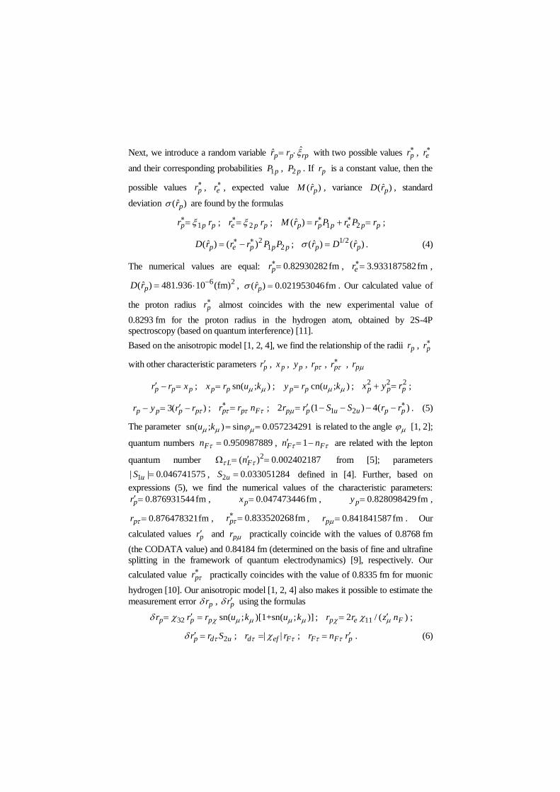
Next, we introduce a random variable ˆˆp p rpr r with two possible values pr , er
and their corresponding probabilities 1pP , 2 pP . If pr is a constant value, then the
possible values pr , er
, expected value ˆ( )pM r , variance ˆ( )pD r , standard
deviation ˆ( )pr are found by the formulas
1p p pr r ; 2e p pr r ; 1 2ˆ( )p p p e p pM r r P r P r ;
21 2ˆ( ) ( )p e p p pD r r r P P ;
1/2ˆ ˆ( ) ( )p pr D r . (4)
The numerical values are equal: 0.82930282fmpr , 3.933187582fmer
,
6 2ˆ( ) 481.936 10 (fm)pD r , ˆ( ) 0.021953046fmpr . Our calculated value of
the proton radius pr almost coincides with the new experimental value of
0.8293 fm for the proton radius in the hydrogen atom, obtained by 2S-4P
spectroscopy (based on quantum interference) [11].
Based on the anisotropic model [1, 2, 4], we find the relationship of the radii pr , pr
with other characteristic parameters pr , px , py , pr , pr , pr
p p pr r x ; sn( ; )p px r u k ; cn( ; )p py r u k ; 2 2 2p p px y r ;
3( )p p p pr y r r ; p p Fr r n ; 1 22 (1 ) 4( )p p u u p pr r S S r r
. (5)
The parameter sn( ; ) sin 0.057234291u k is related to the angle [1, 2];
quantum numbers 0.950987889Fn , 1F Fn n are related with the lepton
quantum number 2( ) 0.002402187L Fn from [5]; parameters
1| | 0.046741575uS , 2 0.033051284uS defined in [4]. Further, based on
expressions (5), we find the numerical values of the characteristic parameters:
0.876931544fmpr , 0.047473446fmpx , 0.828098429fmpy ,
0.876478321fmpr , 0.833520268fmpr , 0.841841587fmpr . Our
calculated values pr and pr practically coincide with the values of 0.8768 fm
(the CODATA value) and 0.84184 fm (determined on the basis of fine and ultrafine
splitting in the framework of quantum electrodynamics) [9], respectively. Our
calculated value pr
practically coincides with the value of 0.8335 fm for muonic
hydrogen [10]. Our anisotropic model [1, 2, 4] also makes it possible to estimate the
measurement error pr , pr using the formulas
32 sn( ; )[1+sn( ; )]p p pr r r u k u k ; 112 / ( )p e Fr r z n ;
2p d ur r S ; | |d ef Fr r ; F F pr n r . (6)
4

Taking into account 11χ 0.181800122 ,
32χ 0.010405201 , | | 0.250425279ef
from [1, 2] and expressions (6) we find estimates of measurement errors
0.009124649fmpr , 0.006902512fmpr , which do not disagree the
experimental estimates of 0.0091 fm from [11], 0.0069 fm from [9], respectively. In
this case, the calculated value of the radius 0.208842481fmdr in our model is
near the mean square radius of the electric charge distribution in the core of nucleons
equal to 0.21 fm [12]. The radius 0.833951278fmFr is related with the
characteristic radii Fr , Lr and the value 0.97597813L by the expressions
F F pr n r ; 2 2 2( ) ( ) ( )F L pr r r ;
2 2( )L L pr r ; 1 (1 )L L F Fn n . (7)
The values of these radii are equal: 0.042980266fmFr , 0.866334751fmLr .
Anomalies in the magnetic moments of leptons can be determined by the influence
of CMB radiation. In this case, relict radiation can lead to effects of renormalization
of the initial parameters: fine structure constant 0 , electron charge e , limiting
speed of photon propagation in vacuum 0c ; rest masses em , m , m and
magnetons B , / 2e m , / 2e m for electron, muon, -lepton,
respectively. The magnetic moments of leptons ˆe , ˆ , ˆ for an
electron, muon, -lepton, respectively, are determined by the expressions
ˆ2 (2 )e e B ; ˆ2 (2 ) ; ˆ2 (2 ) . (8)
Anomalous contributions to magnetic moments and renormalization effects are
described by parameters e , , for electron, muon, -lepton,
respectively, based on the lepton number L
e L HL ; 0/HL HL HE E ; 3HL H eE n E ; 17.21088699N ; (9)
L NL ; 0/NL NL HE E ; NL eE N E ; 0( ) FN N n ; (10)
0.5( )L HL GL ; 0/GL GL HE E ; GL G eE n E . (11)
Additional contributions HL , NL , GL are determined based on the energies
HLE , NLE , GLE and the resting energy of the Higgs boson 0HE . From (9) - (11)
it follows that these additional energies are determined by the numbers of quanta
3Hn , N , Gn and the rest energy of the electron eE . Wherein
3 3 0/ (1 )H Hn n ; 2 2 2
0 01 1 ( ) 1 ( ) χF pn N N ; (12)
3 3 2 3 00.5H H h H An Q n Q n ; 0 ( 1) /A Q gn z z n n ; 2Q Gn n . (13)
Here 8gn , 6Qn , ˆ ˆ 3G G Gn c c and ˆ ˆ 2G G Gn c c
can be
5

interpreted as the numbers of quanta of the gluon, quark, excited, and ground states
of the gravitational fields, respectively; neutrino density 0ν 0.002939801 [4].
Based on (13) we find 3 20.33926863Hn . Further, taking into account (12), (10),
we obtain 3 20.27965049Hn , 0.052340473Fn . Based on equations (9) - (11)
we find the energies 10.36288254 MeVHLE , 8.794747246 MeVNLE ,
1.53299721MeVGLE ; additional contributions 682.88159067 10HL
,
670.33975716 10NL ,
612.26080164 10GL . The found parameters
6/ 2 1159.652705 10e ,
6/ 2 1165.92362110 ,
6/ 2 1177.307902 10
coincide with the data [14] for anomalies of the magnetic moments of leptons.
3 New Hubble Constants
The parameters of active nanoobjects and femtoobjects are related with
cosmological parameters. To describe accelerated expansion of the Universe in
model I [17] and the anisotropic model [1, 2, 4], the Hubble constants 01H , 02H ,
0H , characteristic distances 01L , 02L , 0L , speeds 01 , 02 , 0 were introduced
01 0 01 01 0/ /H c L L ; 02 0 02 02 0/ /H c L L ; 0 0 0/H L . (14)
The values 0 1MpcL , -1 1
01 73.2 km s МpcH , 01 4.0954948GpcL
(distance to supernova type 1a), -1
01 73.2 km s and 02 4.2574359GpcL
(event horizon), -1 1
02 70.415674 km s МpcH , -1
02 70.415674 km s were
obtained on the basis of the analysis of supernova type 1a [3] and measurements by
Cepheids, respectively. The Hubble constant -1 1
0 67.83540245km s МpcH ,
velocity -1
0 67.83540245km s were introduced in [1, 2, 4] to describe the
radiation of gravitational waves, relict photons from binary black holes, neutron
stars based on the expression
0 01/ tH ; 0 01| |tH HQ S ; 0 01 02 01 02 02 01/ / H /HQ H L L . (15)
Here are 0 1.039541282HQ , 01| | 0.039541282S . New experimental data on
the attenuation of γ-rays against an intergalactic background [18] make it
possible to introduce a new Hubble constant 0H, velocity 0
, and matter
density m based on expressions
0 0 0/H L ; 0 01 / tH ; 012tH tH S ; 012 01 02| |S S S . (16)
Here is 02 0.03409S . The numerical values of -1 1
0 67.49443576kms МpcH ,
-10 67.49443576km s , 1( ) / 2 0.141145722m F cn (the parameter
1 0.228071512c is related to the gap in the energy spectrum of relict
6

photons) are close to the experimental data from [18]. From [16] it follows the
connection of parameters 01H , 01 for the accelerated expansion of the
Universe with new parameters 0H, 0
. Our parameters 0H , 0 and new
parameters 0H, 0
are close to the main parameters 0H , 0 of the model
ɅCDM (plane cosmology). In our model 0H , 0 are defined by expressions
0 0 0/H L ; 0 01/ tH ; 0 0 0/tH tH g A An n . (17)
Values -1 1
0 67.30995226km s МpcH , -1
0 67.30995226km s are close to
the parameters of the planar cosmology model.
4 Solar wind and heliopause
The Sun is the source of solar wind (flows of photons and various particles) [19].
Photons achieve the Earth after 8 min, and high-energy particles arrive with a delay
of 100 min [20]. To estimate the characteristic distances and times, we use
0 0 0/ES ES H ES H ESL L Q c t t ; 2 2 2 2
0 0 01 01 02(1 | |) /H Hn Q S , (18)
where 2 2
0 0 0/H Hc n . Taking into account the numerical values of the distance
from the Earth to the Sun 81au 1.495995288 10 kmESL , the limiting speed of
light in a vacuum 5 -1
0 2.99792458 10 kmsc , we find estimates of the refractive
index of the medium 0 1.080646077Hn , the speed of photon propagation in the
medium 5 -1
0 2.883891801 10 kmsH , the distance 0.961962759auESL , and
the times of arrival of photons to the Earth from the Sun in vacuum
480.0293392sESt and in the medium 499.0103147sESt .
To estimate the delay time 0mt of particles, arriving on the Earth from the Sun, we
use the expressions
0 0 02 lnm mt N ; 0 0 0/ n ; 1
0 0
; 2
0 01.5 | |Hn ;
0 0 0ln 2 lnmN n N ; 2 0 10.5H c FQ N n ; 0 0 0/H AN . (19)
Expressions (19) were obtained in the framework of the Dicke theory of
superradiance and describe the main parameters 0 , 0mt of the superradiance
pulse in a medium from a state with the number of particles 0mN .
Based on the numerical values 5
0 3.557716045 10AN , 0 50.182731HzH ,
20| | 0.181800122H , 2 1/ 3HQ , 0.049012111Fn we find estimates of the
frequency 0 141.0532217μHz , relaxation time 0 118.1587096 min ,
fractal parameter 0 1.681800122n , coherent spontaneous relaxation time
0 70.25728449 min , effective numbers of active particles 0 2.331250869N
7
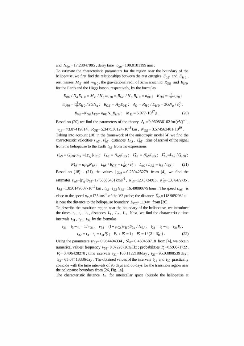
and 0 17.23047995mN , delay time 0 100.0101199 minmt .
To estimate the characteristic parameters for the region near the boundary of the
heliopause, we first find the relationships between the rest energies 0EE and 0HE ,
rest masses EM and 0Hm , the gravitational radii of Schwarzschild GER and 0HR
for the Earth and the Higgs boson, respectively, by the formulas
0 0 0 0 0/ / /E a H E a H GE a H EE N E M N m R N R n ; 2
0 0 0H HE c m ;
20 0 0 / 2H H am c R GN ; 0GE G ER A E ;
40 0 0/ 2 /G H H aA R E GN c ;
0 0GE GE ES E a HR N L n N R ; 275.977 10 gEM . (20)
Based on (20) we find the parameters of the theory 10.960836162fm(eV)GA ,
0 73.87419814En , 185.347530124 10 kmGER ,
103.574563481 10GEN .
Taking into account (18) in the framework of the anisotropic model [4] we find the
characteristic velocities hS , hS , distances hSL , hSL , time of arrival of the signal
from the heliopause to the Earth hSt from the expressions
0 01| |hS H hS efQ ; hS hS ESL N L ; hS hS ESL N L ; 0/hS hS HL L Q ;
0hS H hSN n N ; 2 2
0/ /hS GE hSL R c ; / /hS ES hS ESL L t t . (21)
Based on (18) - (21), the values | | 0.250425279ef from [4], we find the
estimates -1
02| | 17.63386481kmshS ef , 123.6734916hSN , 133.6472735hSN ,
101.850149607 10 kmhSL , 16.49080679 hourhS ES hSt t N . The speed hS is
close to the speed -1
V2 17.5kms of the V2 probe; the distance 118.9692932auhSL
is near the distance to the heliopause boundary V2 119auL from [26].
To describe the transition region near the boundary of the heliopause, we introduce
the times 1t , 2t , 3t , distances 1L , 2L , 3L . Next, we find the characteristic time
intervals 31t , 21t , 32t by the formulas
31 3 1 311/t t t ; 31 02 0 2 0(1 ) /H u AS N ; 21 2 1 31t t t t P ;
32 3 2 31t t t t P ; 1P P ; 031/ (2 )P S . (22)
Using the parameters 02 0.984494334 , 03 0.460458718S from [4], we obtain
numerical values: frequency 31 0.072287263μHz ; probabilities 0.593571722P ,
0.406428278P ; time intervals 31 160.1122188dayt , 21 95.03808539dayt ,
32 65.07413336dayt . The obtained values of the intervals 21t and 32t practically
coincide with the time intervals of 95 days and 65 days for the transition region near
the heliopause boundary from [26, Fig. 1a].
The characteristic distance 3L for interstellar space (outside the heliopause at
8

3 2L L ) is determined from the expressions
3 3L ESL N L ; 3 2(1 )L hL u hSN S N . (23)
Using the parameters 0.000118617hL from [4, 5], hSN from (21), we find the
value 3 119.5712542LN and the estimate of the distance 3 119.5712542auL .
To estimate the distance 1L (inside the heliosphere for 1 2L L ), we use the
characteristic distances eL , L , L for e , , -leptons, respectively,
determined by the expressions
e e ESL N L ; e e hSN n N ; 1(2 ) (1 )e e un S ;
ESL N L ; hSN n N ; 1(2 ) (1 )un S ;
ESL N L ; hSN n N ; 1(2 ) (1 )un S . (24)
Using the parameters e , , from (9) - (11), based on (24) we find the
estimates of distances 118.1796344aueL , 118.1811855auL ,
118.1840014auL . For search of the characteristic distance 2L (as the
heliopause boundary), we consider a random variable 2L with two possible values
3L from (23), 1 eL L from (24) and their corresponding probabilities 01P ,
01P . For expected value 2ˆ( )M L , variance 2
ˆ( )D L , deviation 2ˆ( )L , we have
2 01 3 01 2ˆ( ) eM L P L P L L ;
22 3 01 01
ˆ( ) ( )eD L L L P P ; 1/2
2 2ˆ ˆ( ) ( )L D L ;
01 01 1P P ; 01 01 03 01/ (1 )P S ; 01 1.015268884 . (25)
The numerical values of the distance 2 119.0005661auL and space intervals
32 3 2 0.57068813auL L L , 21 2 0.8209317aueL L L practically coincide
with the characteristic values of 119 au, 0.57 au, 0.82 au, respectively, from [26,
Fig. 1a]. Based on (22), (25), we find the average values of the velocities 21
(inside the heliosphere), 32 (outside the heliopause), the jump in velocities 21
(at the heliopause) and the ratio of velocities 32 21/
21 21 21 31 01 31/ /L t L P t P ; 32 32 32 31 01 31/ /L t L P t P ; 31 3 1L L L ;
21 32 21 ; 32 21 01 01 0 01 0/ / /H HE . (26)
The numerical values are equal: -1
21 14.95635805kms , -1
32 15.18472495kms ,
-121 228.366896ms . We note, that the probabilities 01P and P are coupled
through a conditional probability P , and the ratio of the velocities and the jump in
velocities allow us to introduce probabilities P , P using expressions of the type
9
01P P P ; 03 03 01 01(2 ) / (1 ) 1/ (1 )P S S n ; 1P P ;
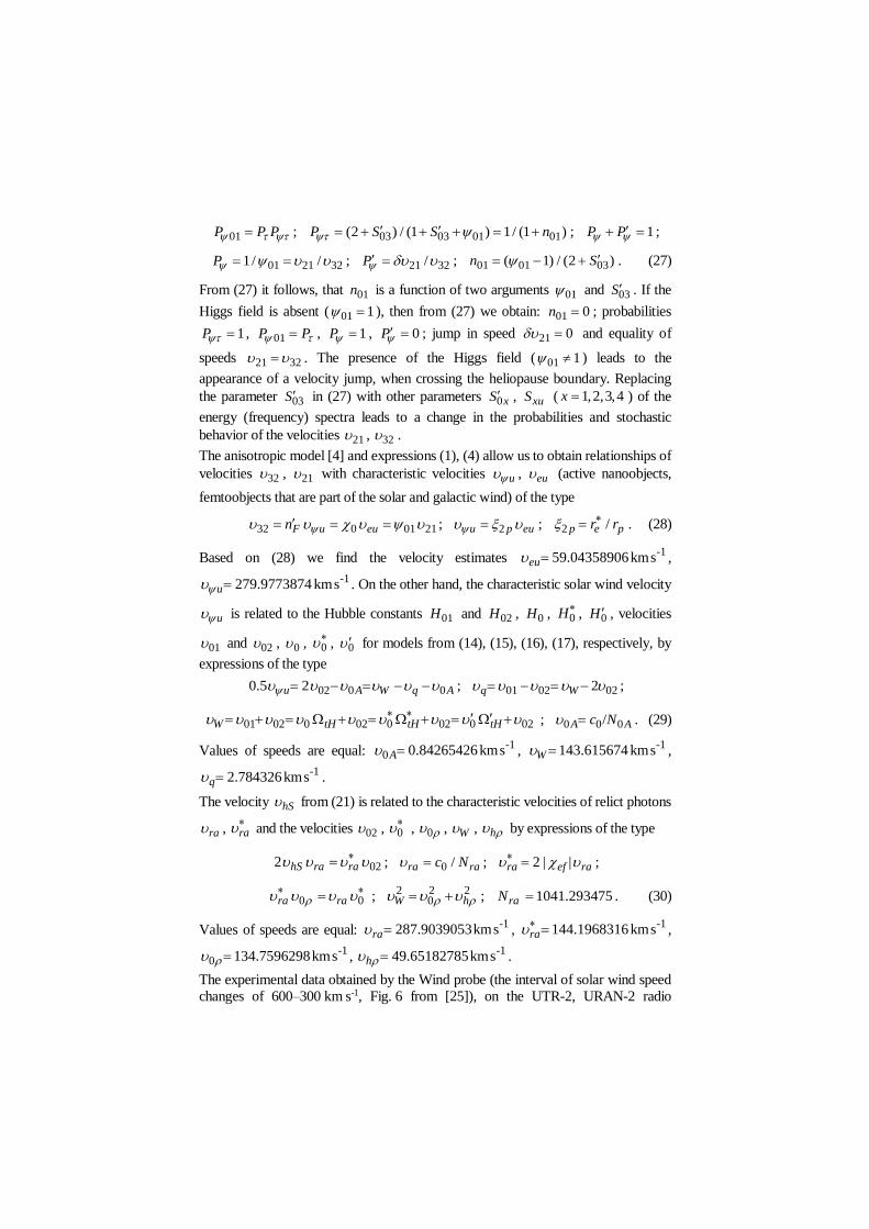
01 21 321/ /P ; 21 32/P ; 01 01 03( 1) / (2 )n S . (27)
From (27) it follows, that 01n is a function of two arguments 01 and 03S . If the
Higgs field is absent ( 01 1 ), then from (27) we obtain: 01 0n ; probabilities
1P , 01P P , 1P , 0P ; jump in speed 21 0 and equality of
speeds 21 32 . The presence of the Higgs field ( 01 1 ) leads to the
appearance of a velocity jump, when crossing the heliopause boundary. Replacing
the parameter 03S in (27) with other parameters 0xS , xuS ( 1,2,3,4x ) of the
energy (frequency) spectra leads to a change in the probabilities and stochastic
behavior of the velocities 21 , 32 .
The anisotropic model [4] and expressions (1), (4) allow us to obtain relationships of
velocities 32 , 21 with characteristic velocities u , eu (active nanoobjects,
femtoobjects that are part of the solar and galactic wind) of the type
32 0 01 21F u eun ; 2u p eu ; 2 /p e pr r . (28)
Based on (28) we find the velocity estimates -159.04358906kmseu ,
-1279.9773874 kmsu . On the other hand, the characteristic solar wind velocity
u is related to the Hubble constants 01H and 02H , 0H , 0H, 0H , velocities
01 and 02 , 0 , 0
, 0 for models from (14), (15), (16), (17), respectively, by
expressions of the type
02 0 00.5 2u A W q A ; 01 02 022q W ;
01 02 0 02 0 02 0 02W tH tH tH ; 0 0 0/A Ac N . (29)
Values of speeds are equal: -1
0 0.84265426kmsA , -1143.615674 kmsW ,
-12.784326kmsq .
The velocity hS from (21) is related to the characteristic velocities of relict photons
ra , ra and the velocities 02 , 0
, 0 , W , h by expressions of the type
022 hS ra ra ; 0 /ra rac N ; 2 | |ra ef ra ;
0 0ra ra ; 2 2 2
0W h ; 1041.293475raN . (30)
Values of speeds are equal: -1287.9039053kmsra ,
-1144.1968316kmsra ,
-10 134.7596298kms ,
-149.65182785kmsh .
The experimental data obtained by the Wind probe (the interval of solar wind speed
changes of 600–300 km s-1, Fig. 6 from [25]), on the UTR-2, URAN-2 radio
10

telescopes (Fig. 5 from [25]) showed, that the solar wind in orbit and beyond the
Earth’s orbit consists of a set of particle flows with different velocities and densities.
The structure of these flows depends on time and solar activity [19, 20]. An analysis
[25] of intermode (intramode) interactions of particles of different flows was
performed by the interplanetary scintillation method based on the behavior of space
and time correlation functions for radiation intensity. The velocities 02 , u
and ra are close to the characteristic velocities of 270, 280 and 290 km s-1 of
separate solar wind modes from [25]. The detailed analysis of the multimode
structure of the solar wind in our model is possible based on spectra of type
2ux u xuS and 2rax ra xuS . From (30) it follows that the velocities 0
and h can be interpreted as both the radial and transverse components of the total
velocity W . The presence of transverse components h of the solar wind near
the Sun is confirmed by experimental data collected by the Parker Solar Probe [21 -
24]. The behavior of the transverse component (Fig. 2 from [22]) is stochastic and
varies in the range from 50 to –50 km s-1. In [24], such a behavior of the slow solar
wind is associated with the presence of equatorial coronal holes in the Sun. A fast
solar wind with speeds 02 occurs near the poles of the Sun.
In our model, it is also possible to describe the multimode structure of the solar and
galactic winds at the crossing of the heliopause based on the velocities eu from
(28), W from (29), ra from (30) and the corresponding velocity spectra. The
experimental data (Fig. 4d from [27], Fig. 2 from [29]) confirm the stochastic
behavior and change in the velocity of solar wind particles when the heliopause
crosses from 150 km s-1 to 100 km s-1. The complex dynamic behavior of the
plasma components (Fig. 3, 4 from [29]) with velocities near eu , 2 eu inside the
heliosphere indicates the presence of a boundary layer near the heliopause.
To estimate the characteristic energies 0A , 0AE , A , effective wavelength A ,
effective number 0nN of particles, we use expressions of the type
0 0 0 0/ /H A A G AE E E N ; 0 0 0 0/ /H A A G nE E E N ;
0 0 0/H G HG n AE E N N N ; 2
0 0 0A A A H GE E E ; /A Aa . (31)
Taking into account 5
0 3.557716045 10AN , 161.031830522 10HGN , a from [6]
we find the estimates: 0 351.4400206 keVA , 0 4.311073329eVAE ,
1.230887363keVA , 1.007114093nmA , 10
0 2.900261036 10nN .
The presence of a multimode structure of the solar and galactic wind, the Higgs field
leads to the replacement A , A by A
, A
by the formulas
A rc bb ; / 2A A Aa R ; /A A GE R A ;
0 1 2(| | )bb A u uS S ; 0 01 02 1 02 22 / ( ) /rc rc A u uE S S . (32)
11

The values are equal: 28.042404 keVbb , 0.04420725rc , 95.290347 meVrc ,
1.239677565 keVA , 0.999972933nmA
, 0.520365996МeVAE . The
energy AE (for solar wind particles inside the heliosphere) is associated with the
energy LE (for galactic wind particles behind the heliopause)
0( )A L g G LE n E ; 0 0 11.5G A c FN n ;
2 2 20 4rc A rcE E ;
2 2 20( ) 4rc A rcE E . (33)
The numerical values are equal: 6
0 4.99501253 10G , 213.0772532МeVLE ,
4.306858745eVrcE , 4.315283797eVrcE . The energy estimates bb , LE
obtained in our model are consistent with the energies of 28 keV, 213 MeV from
[26], and the energy AE is consistent with the energy of 0.5 MeV from [28].
The magnetic characteristics of solar and galactic wind particles have features of the
behavior at the intersection of the heliopause: a jump in the magnetic field from 0.42
to 0.68 nT is observed (Fig. 1a from [27]); components of the magnetic field can
have different signs (Fig. 3 from [27]); the presence of a magnetic barrier (Fig. 4a
from [27]); a change in the direction of the magnetic field components (Fig. 6b, c
from [27]). In our model, to estimate the components of magnetic fields y xB ,
y xB
we use frequency spectra of the type
0/ 2 2y x n y x y xB S ; / 2 2y x n y x y uxB S ; 0,1,2y ;
0 /y y raN ; 2 1 2 1 012/ (1.5 )zgB B n S ; 00 0H ; 02 02 0H . (34)
Here we use the well-known nuclear gyromagnetic ratio / 2 0.6535МHz/kOn
for the deuteron (2H) [12], 0.114317037zgn [4]. Based on (34) we find estimates:
frequencies 2 1 4.4353480mHz ; jump of magnetic fields from 2 1 0.4190147 nTB
to 2 1 0.6787067 nTB at the intersection of heliopause. The numerical values of
the fields deviations of the type 0 1 0 2 0.0804015nTB B B ,
0 1 0 2 0.2019195nTB B B and the sum of the deviations
0.282321nTB B are characteristic of the stochastic behavior of the
magnetic field on time inside the heliosphere (consistent with data Fig. 6 from [27]).
Conclusions
In fractal quantum systems the model femtoobjects, as active objects with sizes
of the order of the classical electron radius, are considered. The main parameters
of the model femtoobject, which are coupled with the known parameters from
quantum electrodynamics and the Higgs boson, are introduced. To take into
12

account the stochastic behavior of the parameters, random variables with two
possible values and the corresponding probabilities are introduced. It was
shown, that the obtained estimates of the proton radius, measurement errors
using the example of the hydrogen atom, and estimates of the anomalies in the
magnetic moments of leptons are consistent with the experimental data.
The parameters of active nanoobjects and femtoobjects are coupled with
cosmological parameters, with new values of the Hubble constants. These active
objects can determine the compound, structure and behavior of the solar wind
(flows of various particles) near the Sun, Earth and in interstellar space (near the
heliopause). The relationships of such active objects with the parameters of the
Higgs boson and the Higgs field are determined. Estimates of the main
parameters are conformed with the experimental data, obtained by the Planck
space observatory (based on Fermi-LAT and Cerenkov telescopes), UTR-2 and
URAN-2 radio telescopes, Parker Solar Probe, Voyager 2 and Voyager 1.
The results can be used to find a solution to the problem associated with the Covid-
2019 virus (based on active femtoobjects and nanoobjects), in cosmic medicine.
References
1. V.S. Abramov. Gravitational Waves, Relic Photons and Higgs Boson in a Fractal
Models of the Universe / C.H. Skiadas and I. Lubashevsky (eds.), 11th Chaotic Modeling and Simulation International Conference, Springer Proceedings in
Complexity. Springer Nature Switzerland AG 2019. P. 1-14.
2. V.S. Abramov. Superradiance of Gravitational Waves and Relic Photons from Binary
Black Holes and Neutron Stars. Bulletin of the Russian Academy of Sciences: Physics, 83, 3, 364-369, 2019.
3. A.G. Riess, A.V. Filippenko, P. Challis et al. Observational Evidence from
Supernovae for an Accelerating Universe and a Cosmological Constant. Astronomical
Journal, 116, 3, 1009-1038, 1998. 4. V.S. Abramov. Active Nanoobjects, Neutrinos and Higgs Fields in Anisotropic
Models of Fractal Cosmology. Bulletin of the Russian Academy of Sciences: Physics,
83, 12, 1516-1520, 2019.
5. V.S. Abramov. Supernonradiative states, neutrino and Higgs Boson in fractal quantum systems. Bulletin of the Russian Academy of Sciences: Physics, 84, 3, 284-288, 2020.
6. V.S. Abramov. Active Nanoobjects, Neutrino and Higgs Boson in a Fractal Models of
the Universe / C.H. Skiadas and Y. Dimotikalis (eds.), 12th Chaotic Modeling and
Simulation International Conference, Springer Proceedings in Complexity. Springer Nature Switzerland AG 2020. P. 1-14.
7. V. Abramov. Super-nonradiative states in fractal quantum systems // XIII International
Workshop on Quantum Optics (IWQO-2019). EPJ Web of Conferences, 220, 2 p.,
2019. 8. O.P. Abramova, A.V. Abramov. Effect of Ordering of Displacement Fields Operators
of Separate Quantum Dots, Elliptical Cylinders on the Deformation Field of Coupled
Fractal Structures. / C.H. Skiadas and I. Lubashevsky (eds.), 11th Chaotic Modeling and Simulation International Conference, Springer Proceedings in Complexity.
Springer Nature Switzerland AG 2019. P. 15-27,
9. R. Pohl, A. Antognini, F. Nez et al. The size of the proton. Nature, 466, 213-217,
2010. 10.A. Beyer, L. Maisenbacher, A. Matveev et al. The Rydberg constant and proton size
13

from atomic hydrogen. Science, 358, 79-85, 2017. 11. N. Kolachevsky. 2S–4P spectroscopy in hydrogen atom: the new value for the
Rydberg constant and the proton charge radius. IWQO – 2019: Collection of abstracts.
Vladimir, September 9 - 14, 2019. Moscow, Trovant, 2019. P. 32. 12. S.V. Vonsovsky. Magnetism of microparticles. Moscow, Nauka, 1973.
13. N. Agafonova, A. Alexandrov, A. Anokhina et al. Final results of the OPERA
experiment on ντ appearance in the CNGS neutrino beam. Phys. Rev. Lett. 120,
211801, 1-7, 2018. 14. R.M. Barnett, C.D. Carone, D.E. Groom et al. Review of Particle Physics. Phys. Rev.
D54, 1, 1-22, 1996.
15. V.S. Abramov. The Higgs Boson in Fractal Quantum Systems with Active
Nanoelements. Bulletin of the Russian Academy of Sciences: Physics, 80, 7,859-865, 2016.
16. V.S. Abramov. Pairs of Vortex-Antivortex and Higgs Boson in a Fractal Quantum
System. CMSIM Journal, 1, 69-83, 2017.
17. V.S. Abramov. Cosmological Parameters and Higgs Boson in a Fractal Quantum System. CMSIM Journal, 4, 441-455, 2017.
18. A. Domínguez, R. Wojtak, J. Finke et al. A New Measurement of the Hubble
Constant and Matter Content of the Universe Using Extragalactic Background Light γ-
Ray Attenuation. The Astrophysical Journal. 885, 2, 137, 2019. 19. N. Schukina. The Sun is the source of life and the cause of catastrophes. Part I. A star
named the Sun. Universe, Space, Time, 8 (145), 4-11, 2016.
20. N. Schukina. The Sun is the source of life and the cause of catastrophes. Part II. Light
giving life. Universe, Space, Time, 9 (146), 16-23, 2016. 21. D.J. McComas, E.R. Christian, C.M.S. Cohen et al. Probing the energetic particle
environment near the Sun, Nature, 576, 223-227, 2019.
22. J.C. Kasper, S.D. Bale, J.W. Belcher et al. Alfvénic velocity spikes and rotational
flows in the near-Sun solar wind. Nature, 576, 228-231, 2019. 23. R.A. Howard, A. Vourlidas, V. Bothmer et al. Near-Sun observations of an F-corona
decrease and K-corona fine structure, Nature, 576, 232-236, 2019.
24. S.D. Bale, S.T. Badman, J.W. Bonnell et al. Highly structured slow solar wind
emerging from an equatorial coronal hole. Nature, 576, 237-242, 2019. 25. N.N. Kalinichenko, M.R. Olyak, A.A. Konovalenko et al. Large-scale structure of
solar wind beyond Earth’s orbit reconstructed by using data of two-site interplanetary
scintillation observations at decameter radiowaves. Kinematics and Physics of Celestial
Bodies, 35, 1(205), 27-41, 2019. 26. S.M. Krimigis, R.B. Decker, E.C. Roelof et al. Energetic charged particle
measurements from Voyager 2 at the heliopause and beyond. Nature Astronomy, 3,
997-1006, 2019.
27. L.F. Burlaga, N.F. Ness, D.E. Berdichevsky et al. Magnetic field and particle measurements made by Voyager 2 at and near the heliopause. Nature Astronomy, 3,
1007-1012, 2019.
28. E.C. Stone, A.C. Cummings, B.C. Heikkila et al. Cosmic ray measurements from
Voyager 2 as it crossed into interstellar space. Nature Astronomy, 3, 1013-1018, 2019. 29. J.D. Richardson, J.W. Belcher, P. Garcia-Galindo et al. Voyager 2 plasma
observations of the heliopause and interstellar medium. Nature Astronomy, 3, 1019-
1023, 2019.
30. D.A. Gurnett, W.S. Kurth. Plasma densities near and beyond the heliopause from the Voyager 1 and 2 plasma wave instruments. Nature Astronomy, 3, 1024-1028, 2019.
14

_________________
13th CHAOS Conference Proceedings, 9 - 12 June 2020, Florence, Italy
© 2020 ISAST
Qubits and fractal structures with elements
of the cylindrical type
Olga P. Abramova, Andrii V. Abramov
Donetsk National University, Donetsk, Ukraine E-mail: [email protected]
Abstract: By the method of numerical simulation, the behavior of the deformation field of both separated and related model fractal structures of a cylindrical type was
investigated. It is shown, that for the considered structures, the behavior of the
deformation field essentially depends on the choice of stochastic processes (realized
during iterations) and on the states of the qubit in the perpendicular plane to the axis of the cylinder. It is shown that the structure of the complex deformation field for a circular
(elliptical) cylinder essentially depends on the initial basic, superposition states of the
qubit. Due to the presence of various qubit states for coupled (using the example of
circular and elliptic cylinders) fractal structures, the appearance of random matrices during iterations is characteristic. There is a need to use commutators and anti-
commutators, products of separate deformation field operators. At this, the structure of
the complex deformation field has own characteristic features of behavior.
Keywords: fractal structure, qubits, random matrices, complex deformation field, ordering of operators, quantum chaos.
1 Introduction
Earlier in [1–3], to describe the total deformation field of coupled fractal
structures in an iterative process, the sum of the displacement field operators of
separate fractal structures was used. The deformation field of the coupled
structure essentially depends on the sequence of separate operators of
displacement fields in the iterative process. On the examples of quantum dots
[4], elliptic [1, 2] and circular [3, 5] cylinders the influence of the ordering of
separate operators of displacement fields on the total deformation field of the
coupled structure was shown. The presence of variable semiaxes and variable
moduli leads to stochastic behavior of the complex deformation field of such
structures. Based on pairs of same fractal structures with opposite orientations
of the deformation fields, complex zero operators were introduced [3. 5]. It is
shown that changes in the order of the sequence of separate operators in the zero
operator for a coupled structure leads to the appearance of a nonzero complex
deformation field. At the same time, noise tracks appear on the background of
stochastic peaks. The noise track is a stochastic ring, the inside region of which
is regular region.
For describe quantum chaos random matrices are used [6]. Elements of random
matrices can be formed as a result of an iterative process. In this case, the need
arises for the use of commutators and anti-commutators, products of separate
15

operators, qubit states [7, 8] of the deformation field. Quantum computers [9 -
12] encode information in qubits. The physical systems that realise qubits can
be any objects having two quantum states. Different nanostructures and
metamaterials [13] can be chosen as active objects. These active objects can be
in superposition qubit states and exhibit stochastic properties, quantum
entanglement.
The aim of this work is to describe the deformation fields of fractal coupled
structures consisting of two separate structures (circular and elliptical cylinders)
with different qubit states. In this case, the deformation fields of coupled
structures are considered as the sum and product (scalar and matrix) of the
deformation fields of separate structures.
2 Description of the deformation field of separate fractal
structures in various qubit states
We consider a model fractal structure (circular or elliptical cylinder), located in
a bulk discrete lattice 1 2 3N N N , whose nodes are given by integers , ,n m j .
By analogy with [1 – 3, 5] nonlinear equations for the dimensionless
displacement function u of the lattice node are
2 20(1 2sn ( , ))u uu k u u k ; (1)
2 (1 ) /uk Q ; 2 1/2 (1 )u uk k ; 0 1 2 3p p p n p m p j ; (2)
2 2 2 2 2 21 0 2 0 3 0( ) / ( ) / ( ) /c c cQ p b n n n b m m m b j j j . (3)
Here 0u is the constant (critical) displacement; a is the fractal dimension of the
deformation field u along the axis Oz ( [0,1]a Î ); variable modules uk , uk are
functions of indices n , m , j nodes of the bulk discrete lattice. The choice of the
positive sign of the module uk is associated with the choice of the second
branch of the displacement function u [14]. Function Q determines the form of the
fractal structure, the type of attractors and take into account the interaction of the nodes of
both in the main plane of the discrete rectangular lattice 1 2N N´ as well as
interplane interactions. The parameters 1b , 2b , 3b , 0n , cn , 0m , cm , 0j , cj
characterize different fractal structures. The choice of function p depends on
the choice of parameters ip , 0,3i . In this paper, we are limited to
consideration of qubit states with 1 0p , 2 0p , 3 0p and shift 0 0p .
The iterative procedure on index n for equations (1) - (3) simulates stochastic
processes on a rectangular discrete lattice with dimensions 1 2N N .
By numerical modelling, it was assumed that 1 240N , 2 240N , 0.5 ,
0 29.537u , 0 1.0423p , 1 2 1b b , 0 121.1471n , 0 120.3267m ,
16
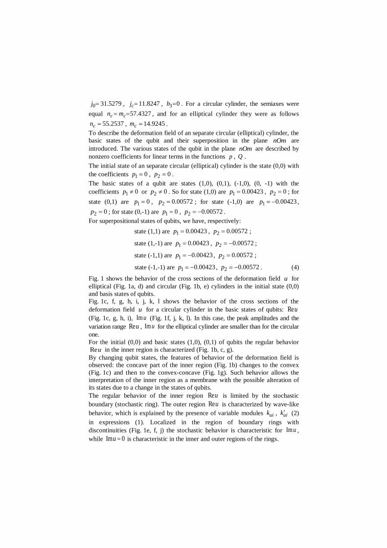
0 31.5279j , 11.8247cj , 3 0b . For a circular cylinder, the semiaxes were
equal 57.4327c cn m , and for an elliptical cylinder they were as follows
55.2537cn , 14.9245cm .
To describe the deformation field of an separate circular (elliptical) cylinder, the
basic states of the qubit and their superposition in the plane nOm are
introduced. The various states of the qubit in the plane nOm are described by
nonzero coefficients for linear terms in the functions p , Q .
The initial state of an separate circular (elliptical) cylinder is the state (0,0) with
the coefficients 1 0p , 2 0p .
The basic states of a qubit are states (1,0), (0,1), (-1,0), (0, -1) with the
coefficients 1 0p or 2 0p . So for state (1,0) are 1 0.00423p , 2 0p ; for
state (0,1) are 1 0p , 2 0.00572p ; for state (-1,0) are 1 0.00423p ,
2 0p ; for state (0,-1) are 1 0p , 2 0.00572p .
For superpositional states of qubits, we have, respectively:
state (1,1) are 1 0.00423p , 2 0.00572p ;
state (1,-1) are 1 0.00423p , 2 0.00572p ;
state (-1,1) are 1 0.00423p , 2 0.00572p ;
state (-1,-1) are 1 0.00423p , 2 0.00572p . (4)
Fig. 1 shows the behavior of the cross sections of the deformation field u for
elliptical (Fig. 1a, d) and circular (Fig. 1b, e) cylinders in the initial state (0,0)
and basis states of qubits.
Fig. 1c, f, g, h, i, j, k, l shows the behavior of the cross sections of the
deformation field u for a circular cylinder in the basic states of qubits: Reu
(Fig. 1c, g, h, i), Im u (Fig. 1f, j, k, l). In this case, the peak amplitudes and the
variation range Reu , Im u for the elliptical cylinder are smaller than for the circular
one.
For the initial (0,0) and basic states (1,0), (0,1) of qubits the regular behavior
Reu in the inner region is characterized (Fig. 1b, c, g).
By changing qubit states, the features of behavior of the deformation field is
observed: the concave part of the inner region (Fig. 1b) changes to the convex
(Fig. 1c) and then to the convex-concave (Fig. 1g). Such behavior allows the
interpretation of the inner region as a membrane with the possible alteration of
its states due to a change in the states of qubits.
The regular behavior of the inner region Reu is limited by the stochastic
boundary (stochastic ring). The outer region Reu is characterized by wave-like
behavior, which is explained by the presence of variable modules uik , uik (2)
in expressions (1). Localized in the region of boundary rings with
discontinuities (Fig. 1e, f, j) the stochastic behavior is characteristic for Im u ,
while Im 0u is characteristic in the inner and outer regions of the rings.
17

a) state (0,0) b) state (0,0) c) state (1,0)
d) state (0,0) e) state (0,0) f) state (1,0)
g) state (0,1) h) state (-1,0) i) state (0,-1)
j) state (0,1) k) state (-1,0) l) state (0,-1)
Fig. 1. The behavior of the cross sections u (top view) depending on the states of
qubits of separate structures: Re [ 1;1]u - (a, b, c, g h, i); Im [ 1;1]u - (d, e, f, j, k,
l). The initial states of qubits (0,0) for elliptical (a, d) and circular (b, e) cylinders.
The basic states of qubits for a circular cylinder (c, f, g - l).
For the other basic states (-1.0), (0, -1) of qubits characteristic stochastic
behavior Reu in the inner region and wave-like behavior in the outer region
(Fig. 1h, i), that indicates a significant alteration of the structures.
For these states Im u has a stochastic structure, localized in the inner region of
the cylinder (Fig. 1k, l), and outside the region Im 0u . The imaginary part
18

Imu indicates the presence of an effective damping. By changing these basis
states, the character of damping changes.
a) state (1,1) b) Re [ 1;1]u c) Im [ 1;1]u
d) state (-1,-1) e) Re [ 1;1]u f) 9 9Im [ 10 ;10 ]u
Fig. 2. Superpositional states of qubits of a separate structure (circular cylinder).
Behavior Reu (a, d) and cross sections (top view) (b, c, e, f)
in the states: (1,1) - (a, b, c); (-1, -1) - (d, e, f).
The presence of superpositional states of qubits in separate structures leads to a
change in the behavior of the complex deformation field. As an example, Fig. 2
shows the behavior Reu (Fig. 2a, d) and cross sections (Fig. 2b, c, e, f) of an
separate structure (circular cylinder) in superposition states of qubits (1,1) and
(-1, -1). The characteristic features of the behavior of the deformation field for
state (1.1) (Fig. 2b, c) are close to state (0,0) (Fig. 1b, e). The characteristic
features the cross sections behavior of deformation field for the state (-1, -1)
(Fig. 2e, f) are close to the states (-1,0) (Fig. 1h, k), (0, -1) (Fig. 1i, l).
However, the behavior Reu for the superposition state (-1, -1) (Fig. 2d) differs
significantly from the characteristic behavior Reu of all other superposition
states of qubits (1,1) (Fig. 2a), (1, -1), (-1,1). Instead of a structure such as a
circular stochastic dislocation (Fig. 2a), a structure like a stochastic funnel
(Fig. 2d) arises. In this case, the amplitudes Reu and Im u for the state (-1, -1)
are significantly smaller than the amplitudes for other states of qubits.
3 Fractal coupled structures with initial states of qubits of
separate structures
Consider the model fractal coupled structures (I,II), (II,I), consisting of two
19

separate structures (I) and (II) with the same initial qubit states (0,0). By
analogy with (1) – (3) nonlinear equations for the dimensionless complex
displacement function u of the lattice node are
2
1Ri
i
u u
; 2 2
0(1 2sn ( , ))Ri i ui i uiu R k u u k ; (5)
2 (1 ) /ui i ik Q ; 2 1/2
(1 )ui uik k ; 0 1 2 3i i i i ip p p n p m p j ; (6)
2 2 2 2 2 21 0 2 0 3 0( ) / ( ) / ( ) /i i i i ci i i ci i i ciQ p b n n n b m m m b j j j . (7)
Here, all parameters have the same meaning as for expressions (1) – (3).
Parameters iR ( =1,2i ) determine the orientation of the deformation fields of
separate structures in a coupled system. For separate structures (I) and (II), the
deformation fields 1Ru u and 2Ru u correspond to the matrices 1RM and
2RM , whose elements are found independently from each other by the iteration
method. In this case, the iterative procedure on index n for equations (5) - (7)
simulates two independent stochastic processes on a rectangular discrete lattice
with dimensions 1 2N N . Earlier in [5], ordered operators of displacement
fields of a coupled structure were introduced as the sum of the operators of
separate structures. Here, for the sum of the matrices 1RM , 2RM the relation is
fulfilled
1 2 2 1R R R R M M M M . (8)
The deformation fields for the coupled structures (I,II), (II,I) correspond to the
ordered operators
(I,II) 1 2R Ru u u u , (II,I) 2 1R Ru u u u (9)
and matrices (I,II)M , (II,I)M , whose elements are found by the iteration
method. The iterative procedure on index n for equations (5) – (7) simulates
two other independent stochastic processes for matrices (I,II)M , (II,I)M . In this
case, the relations are fulfilled
(I,II) 1 2 2 1 (II,I)R R R R M M M M M M ; (I,II) (II,I) 0 M M . (10)
To describe the deviation of the deformation field of the coupled structures (I,II)
and (II,I), we introduce the ordered operator
1 2 2 2 1 1( ( )) ( ( ))R R R Ru u f u u f u , (11)
which corresponds to the matrix M . An iterative procedure on index n
simulate stochastic process for a matrix M , which does not coincide with
stochastic processes for matrices (I,II)M , (II,I)M , 1RM , 2RM . In this case
20
(I,II) (II,I) M M M ; 0 M . (12)
From (12) follows, that stochastic processes for matrices (I,II)M , (II,I)M
become dependent. If in (11) assume 2 2 2( )R Rf u u , 1 1 1( )R Rf u u , then
(I,II) (II,I)M M , what confirms the independence conditions for stochastic
processes (10). Attractors of the deformation field of the coupled fractal
structure are located on the surface, the core of which is determined from the
condition
1 2 0Q Q . (13)
By numerical modeling, it was assumed, that: 0.5i , 0 29.537iu ,
0 1.0423ip , 1 2 1i ib b , 0 121.1471in , 0 120.3267im , 1 1 57.4327c cn m ,
0 31.5279ij , 11.8247cij , 1 2 3 0i i ip p p , 3 0ib . In this case, in fractal
coupled structures (I,II) and (II,I), the structure (I) is a circular cylinder and the
structure (II) is an elliptical cylinder with variable semi-axes 2 2,c cn m . The
variable semiaxes were chosen so that the cross-sectional area of the ellipse
2 2c cS n m did not change and was equal to the cross-sectional area of the
circular cylinder 824.6316S from [2, 3]. For an elliptical cylinder (II), the
semiaxes 2 2,c cn m were defined as follows:
variant 1 are 2 43.0746cn , 2 19.1443cm (the elliptical cylinder is inside the
circular cylinder);
variant 2 are 2 55.2537cn , 2 14.9245cm (the elliptical cylinder approaches
to the circular cylinder along the axis On );
variant 3 are 2 119.9327cn , 2 6.8758cm (the elliptical cylinder extends
beyond the boundaries of the circular cylinder along the axis On ).
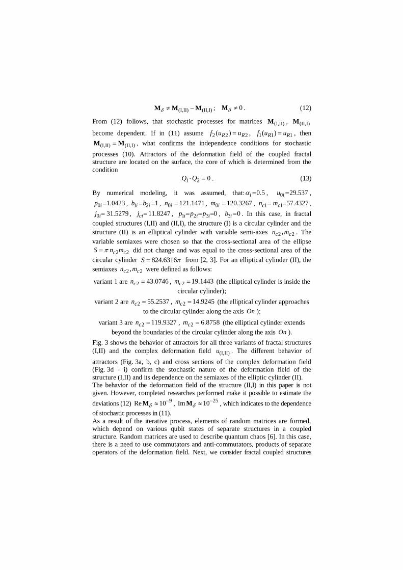
Fig. 3 shows the behavior of attractors for all three variants of fractal structures
(I,II) and the complex deformation field (I,II)u . The different behavior of
attractors (Fig. 3a, b, c) and cross sections of the complex deformation field
(Fig. 3d - i) confirm the stochastic nature of the deformation field of the
structure (I,II) and its dependence on the semiaxes of the elliptic cylinder (II).
The behavior of the deformation field of the structure (II,I) in this paper is not
given. However, completed researches performed make it possible to estimate the
deviations (12) 9Re 10
M , 25Im 10
M , which indicates to the dependence
of stochastic processes in (11).
As a result of the iterative process, elements of random matrices are formed,
which depend on various qubit states of separate structures in a coupled
structure. Random matrices are used to describe quantum chaos [6]. In this case,
there is a need to use commutators and anti-commutators, products of separate
operators of the deformation field. Next, we consider fractal coupled structures
21

(III) and (IV), the deformation fields of which 3u and 4u are described by the
product of the deformation fields of separate structures (I) and (II) with the same
initial qubit states (0,0). The deformation fields of structures (III) and (IV)
correspond to the matrices 3 1 2R R M M M and 4 2 1R R M M M . Here, the dot
symbol describes the operation of ordinary matrix multiplication. Fig. 4 shows the
behavior of the complex deformation field for structures (III) and (IV). In this case,
structure (II) parameters were chosen corresponding to variant 2. The attractors of
structures (III) and (IV) coincide with the attractor from Fig. 3b. Cross sections
(Fig. 4b, e), projections onto the plane nOu (Fig. 4a, d) confirm the stochastic and
fractal behavior of the deformation field of structure (III), which differs significantly
from the behavior of the deformation field of structure (IV) (Fig. 4c, f). This
confirms the non-commutativity the operation of ordinary matrix multiplication
3 4 1 2 2 1 0R R R R M M M M M M .
a) variant 1 b) variant 2 c) variant 3
d) variant 1 e) variant 2 f) variant 3
g) variant 1 h) variant 2 i) variant 3
Fig. 3. The behavior of attractors (a, b, c) and the deformation field u of coupled
structure (I,II): (d, e, f) – (I,II)Re [ 1;1]u , (g, h, i) – (I,II)Im [ 1;1]u cross
sections (top view).
22

a) b) Re [ 1;1]u c) Re [ 1;1]u
d) e) Im [ 1;1]u f) Im [ 1;1]u
Fig. 4. Deformation fields of structures (III), (IV): 3u u (a, d) – projections
onto the plane nOu , (b, e) – cross sections (top view);
4u u (c, f) – cross sections (top view).
Changing the operation of ordinary matrix multiplication on the scalar
multiplication of complex deformation fields leads to the replacement of the
coupled structures (III) and (IV) on structures (V) and (VI). In this case, the
iterative procedure on index n simulates the coupled (dependent) stochastic
processes of the initial independent stochastic processes for separate structures
(I) and (II) with the same initial qubit states (0,0).
The deformation fields of structures (V) and (VI) are described by the functions
5 1 5 2( )R Ru u f u and 6 2 6 1( )R Ru u f u , to which the matrices 5M and 6M
correspond. If by modeling we use independent iterative processes for structures
(I) and (II), then
5 2 2( )R Rf u u ; 6 1 1( )R Rf u u ; 5 1 2 2 1 6R R R Ru u u u u u ; 5 6M M . (14)
Matrix equality confirms the independence of iterative processes.
Fig. 5 shows the behavior of the complex deformation field for structures (V) and
(VI). In this case, structure (II) parameters were chosen corresponding to variant 2.
The attractors of structures (V) and (VI) coincide with the attractor from Fig. 3b.
Cross sections (Fig. 5b, e), projections onto the plane nOu (Fig. 5a, d) confirm
another (compared to Fig. 4) stochastic and fractal deformation field behavior of the
structure (V), which also differs significantly from the deformation field behavior of
the structure ( VI) (Fig. 5c, f). This is due to the dependence of the stochastic
processes ( 5 6M M ).
23

a) b) Re [ 1;1]u c)
d) e) Im [ 1;1]u f)
Fig. 5. Deformation fields of structures (V), (VI): 5u u (a, d) – projections
onto the plane nOu , (b, e) – cross sections (top view);
6u u (c, f) – projections onto the plane nOu .
4 Fractal coupled structures with various superpositional
qubits states of separate structures
Next, we consider the superpositional qubits states of fractal coupled structures (V)
and (VI). The deformation fields of these structures are described by functions
5 1 5 2( )R Ru u f u and 6 2 6 1( )R Ru u f u with the corresponding matrices 5M and
6M , where the scalar multiplication of complex deformation fields of separate
structures (I), (II) is realized. In this case, the iterative procedure on index n
simulates coupled (dependent) stochastic processes for the initial independent
stochastic processes for structures (I) and (II), the deformation fields of which
are described by the functions 1Ru u and 2Ru u . As an example, Fig. 6
shows the behavior of the complex deformation field for structure (V). In this case,
the separate structure (I) is a circular cylinder with parameters as for Fig. 1, and the
parameters of a separate structure (II) (elliptical cylinder) correspond to variant 2
(the elliptical cylinder approaches the circular cylinder along the axis On ). In the
coupled structure (V), the separate structures (I), (II) have the same
superposition qubit states (1,1) (Fig. 6a, b, d, e) and (-1, -1) (Fig. 6c, f). The
behavior of the deformation field of the coupled structure (V) with the same
initial qubit states (0,0) is given on Fig. 5a, b, d, e. The presence of same
superpositional qubit states (1,1) of separate structures in a coupled system
24

(Fig. 6a, b, d, e) leads to a change in the complex deformation field compared to
Fig. 5a, b, d, e: the decrease amplitudes of peaks, the shift of peaks (Fig. 6a, b),
the change of structure (Fig. 6d, e) are observed. An original feature of the
deformation field behavior of the coupled structure (V) with the same
superpositional states (-1, -1) of separate structures is the absence of the
imaginary part of the displacement function in all region ( 5Im 0u ), that
indicates the absence of effective attenuation. This makes it possible to interpret
the coupled structure (V) with the same superpositional states (-1, -1) of the
separate structures (I), (II) as a memory cell. For 5Reu the presence of a
broadened stochastic peak up is characteristic (Fig. 6c). In this case the cross-
sectional structure (Fig. 6f) for state (-1, -1) differs from the cross-sectional
structure (Fig. 6d) for state (1,1).
a) 3Re 10u b) 3Im 10u c) Reu
d) Re [ 1;1]u e) Im [ 1;1]u f) Re [ 1;1]u
Fig. 6. The behavior of the displacement u of the fractal coupled structure (V):
separate structures (I) and (II) have the same superposition qubit states: (1,1) -
(a, b, d, e); (-1, -1) - (c, f).
By changing the superposition qubit states of separate structures (I), (II), one
can change and control the behavior of the complex deformation field of the
coupled structure (V). As an example, Fig. 7 shows the behavior of cross
sections 5Reu of the fractal coupled structure (V), when changing
superposition qubit states of separate structures (I), (II). If structure (I) is in state
(1,1), and the qubit states of structure (II) change (Fig. 7a, b, c), then the
complex deformation field of structure (V) changes significantly compared to
Fig. 6d, e: for sections 5Reu , the effect of mixing of separate trajectories in the
25

inner region, a change in behavior 5Im u are observed. If structure (I) is in the
state (-1, -1), and the qubit states of structure (II) change (Fig. 7d, e, f), then the
complex deformation field of structure (V) in comparison with Fig. 6c, f (where
5Im 0u ) arises. In this case, an alteration of the structure of the inner region
with the formation of stochastic boundary rings, the effect of mixing of
individual trajectories for the cross sections Reu are observed. Using
additional (external or internal) action the transitions of separate structures from
one qubit state to another can be realized.
a) (I):(1,1), (II):(-1,1) b) (I):(1,1), (II):(-1,-1) c) (I):(1,1), (II):(1,-1)
d) (I):(-1,-1), (II):(-1,1) e) (I):(-1,-1), (II):(1,1) f) (I):(-1,-1), (II):(1,-1)
Fig. 7. The behavior of the cross sections Re [ 1;1]u (top view) for fractal
coupled structure (V). Separate structures (I) and (II) have different
superpositional states of qubits.
Similarly, the behavior of the deformation field of the coupled structure (VI),
depending on the qubit states of separete structures (II), (I) was studied. In the
general case, the deformation field of the coupled structure (VI) is complex. In this
case, the conditions
6 5 2 6 1 1 5 2( ) ( ) 0R R R Ru u u f u u f u , 6 5 0 M M , (15)
are satisfied, that is connected with the dependence of this stochastic processes. This
indicates, that the displacement field operators of the separate structures (II), (I) and
(I), (II) do not commute in the coupled structures (VI) and (V). As for structure (V),
a feature of the deformation field behavior of the coupled structure (VI) with the
same superposition states (-1, -1) of separate structures is the absence of
effective attenuation in all region ( 6Im 0u ). For 6Reu the presence of the
26

broadened stochastic peak with a structure close to the peak 5Reu (Fig. 6c) is
also characteristic, but 6 5Re Re 0u u .
Conclusions
By the numerical modelling method the behavior of the deformation field of the
coupled fractal structures (circular and elliptical cylinders) in various (initial,
basic, superpositional) qubit states was investigated. It is shown, that when the
qubit states change, features of the behavior of the complex deformation field of
a separate structure are observed. The regular behavior of the inner region Reu
is limited by the stochastic boundary (stochastic ring), wherein the concave part
of the inner region changes to convex and then to convex-concave. The wave-
like behavior for outer region Reu is characteristic. Such behavior allows the
interpretation of the inner region as a membrane with the possible alteration of
its states due to the change of qubit states. The stochastic behavior for Im u ,
localized in the region of boundary rings with discontinuities is characteristic,
wherein in the inner and outer regions of the rings Im 0u .
For fractal coupled structures with initial states of qubits of separate structures,
the behavior of attractors and the complex deformation field is considered. It is
shown, that the behavior of the deformation field essentially depends on the
choice of stochastic processes realized during iterations. As examples, the
features of the behavior of the deformation fields resulting from the sum, scalar
and matrix products of independent and dependent stochastic processes are
investigated.
Fractal coupled structures with various superpositional states of qubits of
separate structures are considered. It is shown, that the presence of same
superpositional qubit states of separate structures in the coupled system leads to
the change in the complex deformation field: there is the decrease in peak
amplitudes, peak displacement, and the change in structure. The original feature
of the behavior of the deformation field of the coupled structure with the same
superpositional states (-1, -1) of separate structures is the absence of effective
attenuation ( Im 0u ), which allows one to interpret the such structure as the
memory cell.
By changing the superpositional qubit states of separate structures, one can
change and control the behavior of the complex deformation field of the coupled
structure. In this case, for the cross sections Reu , the alteration of the inner
region structure with the formation of stochastic boundary rings, the effect of
mixing of separate trajectories is observed. Using additional (external or
internal) action transitions of separate structures from one qubit state to another
can be realized.
In the general case, the operators of the displacement field of coupled structures
depend on the qubit states of separate structures and do not commute.
The results can be used to describe neural networks with variable parameters, in
medicine when modeling blood vessels, for quantum information processing.
27

References
1. O.P. Abramova. Ordering of the Displacement Field Operators of Separate Quantum Dots, Elliptical Cylinders In Coupled Fractal Structures. Bull. of Donetsk National
Univer., A, 1, 3-14, 2018.
2. O.P. Abramova, A.V. Abramov. Effect of Ordering of Displacement Fields Operators
of Separate Quantum Dots, Elliptical Cylinders on the Deformation Field of Coupled Fractal Structures / C.H. Skiadas and I. Lubashevsky (eds.), 11th Chaotic Modeling
and Simulation International Conference, Springer Proceedings in Complexity.
Springer Nature Switzerland AG 2019. P. 15-26. 3. O.P. Abramova. Complex Zero Operators in Coupled Fractal Structure with Elements
of Cylindrical Type. Bull. of Donetsk National Univer., A, 1, 25-35, 2019.
4. V.S. Abramov. Quantum Dots in a Fractal Multilayer System. Bulletin of the Russian
Academy of Sciences. Physics, 81, 5, 625-632, 2017. 5. O.P. Abramova, A.V. Abramov. Coupled Fractal Structures with Elements of
Cylindrical Type / C.H. Skiadas and Y. Dimotikalis (eds.), 12th Chaotic Modeling
and Simulation International Conference, Springer Proceedings in Complexity.
Springer Nature Switzerland AG 2020. P. 15-26. 6. H.-J. Stöckmann. Quantum Chaos. An Introduction. Philipps-Universität Marburg,
Germany, 2007. 7. A.N. Omelyanchuk, E.V. Ilyichev, S.N. Shevchenko. Quantum Coherent Phenomena
in Josephson Qubits. Kiev, Naukova Dumka, 2013.
8. M.N. Fedorov, I.A. Volkov, Yu.M. Mikhailova. Coutrites and Kukwarts in
Spontaneous Parametric Scattering of Light, Correlation and Entanglement of States. JETP, 142, 1(7), 20-43, 2012.
9. M. Nielsen and I. Chuang. Quantum Computation and Quantum Information.
Cambridge University Press, New York, 2010.
10. D. Boumeister, A. Eckert, A. Zeilinger. Physics of Quantum Information. Springer, New York, 2001.
11. Y. Ozhigov. Quantum Computers Speed Up Classical with Probability Zero. Chaos
Solitons and Fractals, 10, 1707-1714, 1999.
12. D. Castelvecchi. Quantum Computers Ready to Leap out of the Lab. Nature, 541, 9-10, 5 January, 2017.
13. Nonlinearities in Periodic Structures and Metamaterials / ed. Y.S. Kivshar and
N.N. Rozanov, Moscow, Fizmatlit, 2014.
14. V.S. Abramov. Alteration of the Stochastic State of the Deformation Field in the Model Multilayer Nanosystem. Bull. of Donetsk National Univer., A, 2, 81-89, 2014.
28

Fractal atomicity, a fundamental concept in thedynamics of complex systems
Maricel Agop1, Alina Gavrilut2, Lucian Eva3, and Gabriel Crumpei4
1 Department of Physics, “Gheorghe Asachi” Technical University from Iasi,Romania(E-mail: [email protected])
2 Faculty of Mathematics, “Alexandru Ioan Cuza” University of Iasi, Romania(E-mail: [email protected])
3 Prof.Dr. N. Oblu Clinical Emergency Hospital Iasi, Romania (E-mail:[email protected])
4 Faculty of Psychology and Education Sciences, “Alexandru Ioan Cuza” of Iasi,Romania (E-mail: [email protected])
Abstract. Applying a fractal method of analyzing the dynamics of the structuralunits of any complex system, a mathematical concept is built, namely that of fractalatomicity. The construction of such a concept involves defining dynamic variables inthe form of fractal functions, defining scale resolutions, defining a principle of scalecovariance as a fundamental principle of motion, equations of evolution, etc. Finally,some specific mathematical properties of the fractal atom are also established.Keywords: Fractal atomicity, Complex systems dynamics, Fractal functions, Holo-graphic atom.
1 Introduction
The notion of non-atomicity for set functions plays a key role in Measure Theoryand its applications and extensions. For classical measures taking values infinite dimensional Banach spaces, it guarantees the connectedness of range.Even just replacing σ-additivity with finite additivity for measures requiressome stronger non-atomicity property for the same conclusion to hold.
Because of their multiple applications in game theory or mathematical eco-nomics, the study concerning atoms and non-atomicity for additive, respec-tively, non-additive set functions has developed. Particularly, (non)atomic(purely) measures have been studied in different forms due to their specialform and their special properties (Chitescu [8,9], Cavaliere and Ventriglia [7],Gavrilut and Agop [13], Gavrilut and Croitoru [15,17,19], Gavrilut [14,16,18],Gavrilut, Iosif and Croitoru [20], Khare and Singh [31], Li et al. [32, 33], Pap[43-45], Pap et al. [46], Rao and Rao [48], Suzuki [58], Wu and Bo [59] andmany others). Modifications of non-additive Measure Theory (Pap [44,45]) ledto Quantum Measure Theory (Gudder [22-26], Salgado [49], Sorkin [51-54],Surya and Waldlden [55]. In these papers, an extended notion of a measurehas been introduced and certain applications to interference, probability havebeen highlighted (Schweizer and Sklar [50]). In fact, Quantum Measure Theory(introduced by Sorkin [51-54]) represents a generalization of Quantum Theory,where physical predictions are computed from a matrix known as decoherence
29

functional. Quantum measures are an useful tool to describe Quantum Mechan-ics and its applications to Quantum Gravity and Cosmology (Hartle [27,28],Phillips [46]).
Despite the continuous efforts of numerous scientists, reconciling GeneralRelativity with Quantum Theory remains one of the most important openproblems in Physics. The framework of General Relativity suggests that onepromising approach to such a unification will be by means of a reformulation ofQuantum Theory in terms of histories rather than states. Following this idea,Sorkin [51-54], has proposed a history-based framework, which can accommo-date both standard Quantum Mechanics as well as physical theories beyondthe quantum formalism.
As we shall prove in this paper, in such framework, Schrodinger’s equationfrom Quantum Mechanics can be identified with a particular type of geodesic ofthe fractal space. In consequence, fundamental concepts of Quantum Mechan-ics can be extended to similar concepts, but on fractal manifolds. In this paper,we extend the concept of atoms/pseudo-atoms to the concept of fractal minimalatom/fractal pseudo-atom, respectively. We also give characterizations from amathematical viewpoint to these new concepts and we make explicit certainphysical implications. The notion of a fractal minimal atom as a particularcase of fractal atom is also discussed. In this framework, we are looking forcertain physical correspondences in the Quantum Mechanics context.
The present paper is organized as follows. After an Introductory part,Section 2 contains some results concerning the properties of different types ofatoms, introduced from the Quantum Measure Theory mathematical perspec-tive. Certain physical implications and interpretations are provided. In Section3, elements of Fractal Mechanics are provided in order to build the backgroundfor extending the notions that are specific to atomicity, to those involving frac-tal atomicity. From this perspective, new concepts as that of a fractal minimalatom is introduced and some of its properties are discussed in Section 4.
2 Types of atoms in the mathematical approach
In what follows, T denotes an abstract nonvoid set and C a ring of subsets ofT . Suppose (V,+, ·) is a real linear space, with the origin 0.
If p ∈ N∗, then by i = 1, p we usually mean i ∈ 1, 2, ..., p.Definition 2.1 (Gavrilut and Agop [13]) Let m : C → V be a set function,
with m(∅) = 0. m is said to be:
(i) finitely additive if m(n∪i=1Ei) =
n∑i=1
m(Ei), for any arbitrary pairwise
disjoint sets (Ei)i∈1,2,...,n ⊂ C, n ∈ N∗;(ii) null-additive1 if m(E ∪ F ) = m(E), for every disjoint E,F ∈ C, with
m(F ) = 0;(iii) null-additive2 if m(E ∪F ) = m(E), for every E,F ∈ C, with m(F ) =
0;(iv) null-null-additive if m(E ∪ F ) = 0, for every E,F ∈ C, with m(E) =
m(F ) = 0;(v) null-equal if m(E) = m(F ), for every E,F ∈ C, with m(E ∪ F ) = 0;
30

(vi) diffused if m(t) = 0, whenever t ∈ C.Definition 2.2 (Gavrilut et al. [20]) If V is, moreover, a Banach lattice,
a set function m : C → V , with m(∅) = 0, is said to be:
(i) null-monotone if for every E,F ∈ C, with E ⊆ F , if m(F ) = 0, thenm(E) = 0;
(ii) monotone (or, fuzzy) if m(E) ≤ m(F ), for every E,F ∈ C, with E ⊆F ;
(iii) a submeasure (in the sense of Drewnowski [11]) if m is monotone andsubadditive, i.e., m(E ∪ F ) ≤ m(E) + ν(F ), for every (disjoint) E,F ∈ C;
(iv) σ-additive (or, a (vector) measure) if m(∞∪n=1
En) = limn→∞
n∑k=1
m(Ek),
for every pairwise disjoint sets (En)n∈N∗ ⊂ C, with∞∪n=1
En ∈ C.Definition 2.3 If A is an arbitrary σ-algebra of T and if m : A → R+ is
a measure on A, with m(T ) = 1, then:
(i) The space (T,A,m) is said to be a sample space and m is said to be aprobability measure;
(ii) The elements of T are called sample points or outcomes and the ele-ments of A are called events.
In this case, for every E ∈ A,m(E) is interpreted as the probability of theevent E to occur.
Remark 2.4 (i) The notion of a null-equal-measure has the following phys-ical interpretation (Gavrilut and Agop [13]): in the situation involving destruc-tive interference, in order for two waves to produce complete destructive in-terference, thereby “cancelling out” each other, their original amplitudes musthave been equal.
(ii) If m(T ) > 0, then one can immediately generate a probability measureby means of a normalization process.
Remark 2.5 I) (i) One observes that a set function m : C → V is diffused ifthe measure of any singleton of the space is null. This means in the constructionof a physical theory, the vacuum condition of the matter should be consideredas its complement.
(ii) Shannon’s entropy is a subadditive real-valued set function [5].
(iii) If V is a Banach lattice, T = t1, t2, ..., tn, n ∈ N∗, is an arbitraryfinite metric space and m : P(T )→ V (or, more general, if T is a T1-separatedtopological space, B is the Borel σ-algebra of T generated by the lattice of allcompact subsets of T and m : B → V ) is null-additive and diffused, thenm(T ) = 0 (i.e., the space T is composed of particles which annihilate one eachother).
II) If m : C → V is null-monotone, then:
(i) m is null-additive1 if and only if it is null-additive2. In this case, mwill be simply called null-additive.
(ii) If m is null-null-additive, then it is null-equal.
Definition 2.6 (Gavrilut and Croitoru [15,17,19]) Let m : C → R+ be aset function, with m(∅) = 0.
31

(i) A set E ∈ C is said to be an atom of ν if m(E) > 0 and for everyF ∈ C, with F ⊆ E, we have m(F ) = 0 or m(E\F ) = 0 (in a certain sense,an atom can be interpreted as being a black hole);
In consequence, an atom is a measurable set which has positive “measure”and contains no set of smaller positive “measure”. In fact, the main examplesof atomsare singletons that have positive “measure”.
(ii) m is said to be non-atomic (or, atomless) if it has no atoms (i.e., forevery E ∈ C with m(E) > 0, there exists F ∈ C, F ⊆ E, such that m(F ) > 0and m(E\F ) > 0);
(iii) A set E ∈ C is called a pseudo-atom of ν if m(E) > 0 and F ∈ C,F ⊆ E implies m(F ) = 0 or m(F ) = m(E);
(iv) m is said to be non-pseudo-atomic if it has no pseudo-atoms (i.e., forevery E ∈ C with m(E) > 0, there exists F ∈ C, F ⊆ E, such that m(F ) > 0and m(E) 6= m(F ));
(v) m is said to be finitely purely atomic if there is a finite family (Ei)i∈1,2,...,n
of pairwise disjoint atoms of m so that T =n∪i=1Ei (in this case, the space T
is a finite collection of pairwise disjoint atoms).I is well-known that the Lebesgue measure on the real line has no atoms.
It is also that the entropy of a non-atomic measure must be infinite, while theentropy of an atomic measure vanishes. The following statements easily follow:
Proposition 2.7 Suppose m : C → R+ is so that m(∅) = 0.(i) If m is finitely additive, then E ∈ C is an atom of m if and only if E
is a pseudo-atom of m.(ii) Any t ⊆ T , provided t ∈ C and m(t) > 0, is an atom of m.(ii) If m is null-additive1, then every atom of m is also a pseudo-atom.
The converse is not generally valid.Example 2.8 Let T = t1, t2 be a finite abstract space composed of two
elements.(i) We consider the set function m : P(T ) → R+ defined for every E ⊂ T
by m(E) =
2, E = T1, E = t1
0, E = t2 or E = ∅..
Then T is an atom and it is not a pseudo-atom of m.
(ii) We define m : P(T )→ R+ by m(E) =
1, E 6= ∅0, E = ∅ , for every E ⊂ T.
Then m is null-additive and T = t1, t2 is a pseudo-atom of m, but it isnot an atom.
(iii) Let be T = 1, 2, ...10 and m : P(T )→ R+, m(A) = cardA, ∀A ⊆ T .Then each of the singletons i, i ∈ 1, ..., 10 is an atom.
(iv) Let T be a countable set, A = A ⊆ T ; A is finite or T \ A is finite and m : A → R+,
m(A) =
0, A is finite1, T \A is finite
,∀A ∈ A.
Then every set A ∈ A so that T \A is finite is an atom of m.
32

(v) On T = R, let be the algebra A = ∅, T and m : A → R+, m(∅) = 0,m(R) = 1. Then R is an atom and obviously it is not a singleton set.
Proposition 2.9 If m : C → R+ is null-monotone and null-additive andif E ∪ F is an atom of m, then E,F are m-compatible that is, the followingproperty holds: m(E∪F )+m(E∩F ) = m(E)+m(F ) (thus, any two componentsof an atom must be compatible).
Proof. 1. If m(E) = 0, then m(E ∩ F ) = 0 and m(E ∪ F ) = m(F ), so theconclusion follows.
2. If m(E) > 0, then by Proposition 2.7 - (i) E is an atom, too andm((E ∪ F )\E) = m(F\E) = 0. Since F = (F\E) ∪ (F ∩ E), then m(F ) =m(E ∩ F ) and since E ∪ F = E ∪ (F\E), we get m(E ∪ F ) = m(E).
In what follows, let K be the lattice of all compact subsets of a locallycompact Hausdorff space T and B be the Borel σ-algebra generated by K. Insuch framework, the following definition is consistent:
Definition 2.10 (Pap [43-45]) m : B → R+ is said to be regular if forevery E ∈ B and every ε > 0, there exist K ∈ K and an open set D ∈ B suchthat K ⊂ E ⊂ D and m(D\K) < ε.
Theorem 2.11 (Pap [43-45]) Suppose m : B → R+ is a monotone null-additive regular set function. If E ∈ B is an atom of m, there exists only onepoint e ∈ E so that m(E\e) = 0 (and so, m(E) = m(e).
Remark 2.12 The previous theorem has the following physical interpreta-tion: in an atom, the entire ”information” is concentrated in each of its points.
3 Fractal Theory of Motion
As a rule, the classical models used in the description of the dynamics of thesystems are based on the assumption, otherwise unjustified, of the differentia-bility of the variables that describe them. The success of these models mustbe understood gradually / sequentially, on “”domains” in which the differen-tiability and integrability are still valid. But the differentiable and integrablemathematical procedures “suffer” when we want to describe the dynamics ofthe systems, because only these ones “support” and “operate” with nonlinear-ities and chaoticities.
In order to describe dynamics, while still being dependent on the differ-entiable and integrable mathematical procedures, it is necessary to explicitlyintroduce the scale resolution in the expressions of the physical variables thatdescribe them and implicitly in the expressions of the fundamental equationsthat govern these dynamics. This means that any variable, used in describingthe dynamics of the systems, dependent in the classical sense, both on thespatial and time coordinates, depends, in the context mentioned above, on thescale resolution. In other words, instead of “operating” for example with a sin-gle variable described by a strictly non-differentiable mathematical function,we will “operate” only with approximations of this mathematical function ob-tained by mediating it at different scale resolutions. Consequently, any variabledesigned to describe system dynamics will “function” as the limit of a family ofmathematical functions, this being non-differentiable for a zero-scale resolutionand differentiable for a non-zero scale resolution.
33
This way of describing the dynamics of the systems, where any “explici-tation” of dynamics is done at finite scale resolution, obviously implies boththe development of a new geometrical structure and of models conforming tothese geometrical structures for which the laws of motion, invariant to spatialand temporal transformations, are ” integrated ” with scale laws invariant totransformations of scale resolution. In our opinion, such a geometric structurecan be based on the concept of fractal, and the corresponding physical model,the Multifractal Theory of Motion in the form of Scale Relativity Theory witharbitrary and constant fractal dimension [36].
Let us suppose that on a fractal space-time manifold the motions of systemstake place on fractal curves. Then:
Remark 3.1. Any fractal curve is explicitly scale resolution dependent(which will be referred as δτ). Its length tends to infinity when its proper timeinterval, ∆τ , tends to zero (an extension of the Lebesgue theorem on a fractalspace-time manifold).
Remark 3.2. In the limit ∆τ → 0, a curve in a fractal space-time man-ifold is a zig-zagged as one can imagine. Thus, it exhibits the property ofself-similarity in all its points of a fractal space-time manifold, which can betranslated into an extension property of holography (every part of a fractalspace-time manifold reflects the whole of the same space-time manifold).
Remark 3.3. The differential proper time reflection invariance of anyvariable is broken. Then every variable Q(τ) is replaced by the fractal vari-able Q(τ, dτ) explicitly dependent on the proper time resolution interval whosederivative is undefined only in the limit, ∆τ → 0. As a consequence, twoderivatives of every fractal variable as explicit functions of τ and dτ will bedefined. For example, the two derivatives of the 4-coordinate Xµ(τ,∆τ) takesthe form:
d+Xµ
dτ= lim∆τ→0+
Xµ(τ +∆τ,∆τ)−Xµ(τ,∆τ)
∆τ
d−Xµ
dτ= lim∆τ→0−
Xµ(τ,∆τ)−Xµ(τ −∆τ,∆τ)
∆τ(1)
The sign + corresponds to the forward process and the sign − to the back-wards one.
Remark 3.4. The differential of 4-coordinate dXµ(τ,∆τ) can be expressedas the sum of two differentials, one not scale dependent, d±x
µ(τ)), and otherscale dependent, d±ξ
µ(τ, dτ)), i.e.,
d±Xµ(τ,∆τ) = d±x
µ(τ) + d±ξµ(τ, dτ); (2)
Remark 3.5. d±ξµ satisfies the equation
d±ξµ(τ, dτ) = λµ±(dτ)1/f(α) (3)
where λµ± are constant coefficients whose statistical significance will be givenin what follows, f(α) is the singularity spectrum of order α, α is the singularityindex and DF is the fractal dimension of the motion curves from the fractalspace-time manifold.
34

Remark 3.6. There are many modes and thus various selection of defini-tions of fractal dimensions: fractal dimension in the Kolmogorov sense, fractaldimension in the Hausdorff-Besikovici sense etc. Selecting one of these defini-tions and operating with it in the dynamics of systems, the value of the fractaldimension must be constant and arbitrary: DF < 2 for correlative processes,DF > 2 for non-correlative processes etc. In such conjecture we can identify notonly the “areas” of the dynamics of the system that are characterized by a cer-tain fractal dimension, but also the number of “areas” whose fractal dimensionsare situated in an interval values. Moreover, through the singularity spectrumwe can identify “classes of universality” in the dynamics of the system, evenwhen strange attractors have various aspects.
Remark 3.7. The differential proper time reflection invariance is recoveredby combining the derivatives d+/dτ and d−/dτ in the fractal operator (Cressonprocedure):
d
dτ=
1
2(d+ + d−dτ
)− i
2(d+ − d−dτ
) (4)
Applying, for example, the fractal operator to the 4-coordinate Xµ yieldsthe 4-complex velocity:
V µ =dXµ
dτ=
1
2(d+X
µ + d−Xµ
dτ)− i
2(d+X
µ − d−Xµ
dτ) = V µ − iUµ (5)
with
V µ =1
2(vµ+ + vµ−), Uµ =
1
2(vµ+ − v
µ−), vµ+ =
d+xµ + d+ξ
µ
dτ, vµ− =
d−xµ + d−ξ
µ
dτ
The real part V µ is scale resolution independent, while the imaginary oneUµ is scale resolution dependent.
Remark 3.8. An infinite number of geodesics can be found relating anypair of points of a fractal space-time manifold, and this is true on all scale reso-lutions of the physical system dynamics. Then, in the fractal space-time mani-fold, all the entities of the system are substituted with the geodesics themselvesso that any external constraint can be interpreted as a selection of geodesics inthe same fractal space-time manifold.
Remark 3.9. The infinity of geodesics in the bundle, their multifractal-ity, the two values of the derivative etc., imply a generalized statistical fluid-like description (fractal fluid). Thus, one provides the multifractalisation typethrough stochastic processes. For example, we can choose the average of d±X
i
in the form< d±X
i >≡ d±xi (6)
which by (2) implies< d±ξ
i >= 0
Theorem 3.10. The transition from the dynamics of the Special Relativityto the dynamics of Multifractal Theory of Motion in the form of Scale Relativity
35

Theory on a fractal space-time manifold can be described through the scalecovariant derivative:
d
dτ= ∂τ + V µ∂µ +
1
4(dτ)(2/f(α))−1Dµνaµaν (7)
whereDµν = dµν − idµν
dµν = λµ+λν+ − λ
µ−λ
ν−, d
µν= λµ+λ
ν+ + λµ−λ
ν−
(8)
Proof. The proof of the above statements is given in [3].Remark 3.11. If the multifractality of the motion curve is achieved
through Markov type stochastic process
λµ+λν+ = λµ−λ
ν− = −ληµν (9)
where ηµν is the Minkowski metric, then the scale covariant derivative (8) takesthe form
d
dτ= ∂τ + V µ∂µ + i
λ
2(dτ)(2/DF )−1∂µaµ (10)
Remark 3.12. Applying the scale covariant operator to the complex ve-locity (5), the geodesics equation on a fractal space-time is obtained:
dV µ
dτ= ∂τ V
µ + V ν∂ν Vµ +
1
4(dτ)(2/f(α))−1Dαβ∂α∂βV
µ ≡ 0 (11)
Remark 3.13. Through separation of motions on scale resolutions (the realpart from the imaginary one) on a fractal space-time, the geodesics equationin real terms becomes:
dV µ
dτ = ∂τVµ + V ν∂νV
µ − Uν∂νUµ + 14 (dτ)(2/f(α))−1dαβ∂α∂βV
µ−− 1
4 (dτ)(2/f(α))−1dαβ∂α∂βU
µ = 0dUµ
dτ = ∂τUµ + V ν∂νU
µ + Uν∂νVµ + 1
4 (dτ)(2/f(α))−1dαβ∂α∂βUµ+
+ 14 (dτ)(2/f(α))−1d
αβ∂α∂βV
µ = 0
(12)
Theorem 3.14. Choosing the 4-complex velocity from (5) in terms of ascalar complex field Ψ,
V µ = iλ(dτ)(2/f(α))−1∂µ lnΨ (13)
the geodesics of a fractal space-time manifold in the case of multifractalisationby means of Markovian stochastic processes, for a null value of the integrationconstant takes the form of the generalized Schrodinger type equation
λ2(dτ)(4/f(α))−2∂µ∂µΨ + iλ∂τΨ = 0 (14)
Remark 3.15. For non-relativistic dynamics in 3D space on Peano typecurve, f(α) ≡ DF = 2, at Compton scale resolution, λ = ~/2m0, with ~ thePlanck reduced constant and m0 the rest mass of the particle, from (13) itresults the standard Schrodinger equation
~2
2m0∂i∂
iΨ + i~∂τΨ = 0 (15)
36

4 From the standard mathematical atom to the fractalatom by means of a physical procedure
Let T be an abstract nonvoid set, G a lattice of subsets of T and m : G → R+ anarbitrary set function with m(∅) = 0. Evidently, one can immediately generalizethe notions of a pseudo-atom / minimal atom, respectively, to this context whenG is only a lattice and not necessarily a ring.
Example 4.1. (i) It T is a nonempty metric space, then the Hausdorffdimension dimHaus : P(T )→ R (Mandelbrot [34]) is a monotone real function.Evidently, dimHaus(∅) = 0.
(ii) For every d ≥ 0, the Hausdorff measure Hd : P(T )→ R is a submeasure.Remark 4.2. (i) The union of two sets E and F having the fractal dimen-
sions DE , respectively, DF , has the fractal dimension DE∪F = maxDE , DF ;(ii) The intersection of two sets E and F having the fractal dimensions DE ,
respectively, DF has the fractal dimension DE∩F = DE + DF − d, where d isthe embedding Euclidean dimension (Iannaccone and Khokha [29]).
The following definition is then consistent:Definition 4.3. A pseudo-atom/minimal atom, respectively, E ∈ G of m
having the fractal dimension DE is said to be a fractal pseudo-atom/fractalminimal atom, respectively.
Therefore, we can give:Proposition 4.4. If E,F ∈ G are fractal pseudo-atoms of m and if m(E ∩
F ) > 0, then E ∩ F is a fractal pseudo-atom of m and m(E ∩ F ) = m(E) =m(F ).
Conclusions
The main conclusions of the present paper are the following:i) (Pseudo)-atomicity is treated from the Quantum Measure theory math-
ematical perspective and several physical applications are given;ii) Minimal atomicity in correspondence with Quantum Measure Theory is
also discussed. In such context, some physical applications are provided;iii) The concept of atomicity (and, particularly, that of minimal atomicity)
is extended in the form of fractal atomicity, respectively, fractal minimal atom-icity. Some mathematical properties of fractal minimal atomicity are given. Insuch approach, an inverse method with respect to the common developmentsconcerning the atomicity concept has been used, observing that Quantum Me-chanics identifies as a particular case of Fractal Mechanics for a given scaleresolution. Precisely, we talk about a fractality through Markov type stochas-tic processes, in which case the standard Schrodinger equation identifies withthe geodesics of a fractal space for motions of a complex system structural unitson Peano type curves at Compton scale resolution.
The concept of fractal atomicity introduces a minimal code which couldcorrespond to the DNA that is specific to each person. In this paper, we intro-duced the basis for a multivalent logic, which could open new perspectives ingenomics for instance, in the decipher of the intimate mechanisms at biostruc-tures level.
37

References
1. M. Agop, A. Gavrilut, E. Rezus, Implications of Onicescu’s informational energyin some fundamental physical models, International Journal of Modern PhysicsB, 29, 1550045 (2015) [19 pages], DOI: 10.1142/S0217979215500459.
2. M. Agop, A. Gavrilut, G. Crumpei, B. Doroftei, Informational Non-differentiableEntropy and Uncertainty. Relations in Complex Systems, Entropy, 2014, 16,6042-6058.
3. M. Agop, A. Gavrilut, G. Stefan, B. Doroftei, Implications of Non-differentiableEntropy on a Space-Time Manifold, Entropy, 2015, 17, 2184-2197.
4. M. Agop, A. Gavrilut, V.P. Paun, D. Filipeanu, F.A. Luca, C. Grecea, L.Topliceanu, Fractal Information by Means of Harmonic Mappings and SomePhysical Implications, Entropy 2016, 18, 160.
5. K.M. R. Audenaert, Subadditivity of q-entropies for q > 1, J. Math. Phys. 48(2007), 083507.
6. D. Barbilian, Die von einer Quantik induzierte Riemannsche Metrik, Comptes Ren-dus de l’Academie Roumaine des Sciences, Vol. 2, p. 198, 1937.
7. P. Cavaliere, F. Ventriglia, On nonatomicity for non-additive functions, Journal ofMathematical Analysis and Applications, Vol. 415, 1 (2014), 358-372.
8. I. Chitescu, Finitely purely atomic measures and Lp-spaces, An. Univ. BucurestiSt. Natur. 24 (1975), 23-29.
9. I. Chitescu, Finitely purely atomic measures: coincidence and rigidity properties,Rend. Circ. Mat. Palermo (2) 50 (2001), no. 3, 455-476.
10. N. Dinculeanu, Measure Theory and Real Functions (in Romanian), Didactic andPedagogical Publishing House, Bucharest, 1964.
11. L. Drewnowski, Topological rings of sets, continuous set functions, Integration, I,II, III, Bull. Acad. Polon. Sci., 20 (1972), 269-276, 277-286, 439-445.
12. H. Flanders, Differential Forms with Applications to the Physical Science, DoverPublication, New York, 1989.
13. A. Gavrilut, M. Agop, An Introduction to the Mathematical World of Atomicitythrough a Physical Approach, ArsLonga Publishing House, Iasi, 2016.
14. A. Gavrilut, Regular Set Multifunctions, Pim Publishing House, Iasi, 2012.15. A. Gavrilut, A. Croitoru, Non-atomicity for fuzzy and non-fuzzy multivalued set
functions, Fuzzy Sets and Systems, 160 (2009), 2106-2116.16. A. Gavrilut, Fuzzy Gould integrability on atoms, Iranian Journal of Fuzzy Systems,
Vol. 8, No. 3, (2011), 113-124.17. A. Gavrilut, A. Croitoru, On the Darboux Property in the Multivalued Case, An-
nals of the University of Craiova, Math. Comp. Sci. Ser., Vol. 35 (2008), 130-138.18. A. Gavrilut, Non-atomicity and the Darboux property for fuzzy and non-fuzzy
Borel/Baire multivalued set functions, Fuzzy Sets and Systems, 160 (2009), 1308-1317, Erratum in Fuzzy Sets and Systems, 161 (2010), 2612-2613.
19. A. Gavrilut, A. Croitoru, Pseudo-atoms and Darboux property for set multifunc-tions, Fuzzy Sets and Systems, Vol. 161, 22 (2010), 2897-2908.
20. A. Gavrilut, A. Iosif, A. Croitoru, The Gould integral in Banach lattices, Positiv-ity, Vol. 19, 1 (2015), 65-82.
21. A. Grigorovici, E.S. Bacaita, V.P. Paun, C. Grecea, I. Butuc, M. Agop, O. Popa,Pairs Generating as a Consequence of the Fractal Entropy: Theory and Applica-tions, Entropy 2017, 19, 128; DOI:10.3390/e19030128.
22. S. Gudder, Quantum measure theory, Mathematica Slovaca, 60 (2010), 681-700.23. S. Gudder, Quantum measure and integration theory, J. Math. Phys. 50, (2009),
123509.
38

24. S. Gudder, Quantum integrals and anhomomorphic logics, arXiv: quant-ph(0911.1572), 2009.
25. S. Gudder, Quantum measures and the coevent interpretation, Rep. Math. Phys.67 (2011), 137-156.
26. S. Gudder, Quantum measures and integrals.27. J.B. Hartle, The quantum mechanics of cosmology, 1989, Lectures at Winter
School on Quantum Cosmology and Baby Universes, Jerusalem, Israel, Dec 27,1989 - Jan 4, 1990.
28. J.B. Hartle, Spacetime quantum mechanics and the quantum mechanics of space-time, in Proceedings of the Les Houches Summer School on Gravitation andQuantizations, Les Houches, France, 6 Jul - 1 Aug 1992, eds J. Zinn-Justin, andB. Julia, North-Holland (1995), arXiv:gr-qc/9304006.
29. P.M. Iannaccone, M. Khokha, Fractal Geometry in Biological Systems: An Ana-litical Approach, 1995.
30. E.T. Jaynes, The well posed problem, Foundations of Physics, Vol. 3 (1973), 477-493.
31. M. Khare, A.K. Singh, Atoms and Dobrakov submeasures in effect algebras, FuzzySets and Systems, Vol. 159, 9 (2008), 1123-1128.
32. J. Li, R. Mesiar, E. Pap, Atoms of weakly null-additive monotone measures andintegrals, Information Sciences, 2014, 134-139.
33. J. Li, R. Mesiar, E. Pap, E.P. Klement, Convergence theorems for monotonemeasures, Fuzzy Sets and Systems, Vol. 281, 2015, 103-127.
34. B.B. Mandelbrot, The Fractal Geometry of Nature (Updated and augm. ed.),W.H. Freeman, New York, 1983.
35. N. Mazilu, M. Agop, Skyrmions. A Great Finishing Touch to Classical NewtonianPhilosophy, World Philosophy Series, Nova Science Publishers, New York, 2011.
36. I. Merches, M. Agop, Differentiability and Fractality in Dynamics of PhysicalSystems, World Scientific, 2015.
37. R. Mesiar, J. Li, Y. Ouyang, On the equality of integrals, Information Sciences,393 (2017), 82-90.
38. O.D. Michel, B.G. Thomas, Mathematical Modeling for Complex Fluids andFlows, Springer, New York, 2012.
39. M. Mihaileanu, Differential, Projective and Analytical Geometry (in Romanian),Didactic and Pedagogical Publishing House, Bucharest, 1972.
40. M. Mitchell, Complexity: A Guided Tour, Oxford University Press, Oxford, 2009.41. L. Nottale, Scale Relativity and Fractal Space-Time. A New Approach to Unifying
Relativity and Quantum Mechanics, Imperial College Press, London, 2011.42. Y. Ouyang, J. Li, R. Mesiar, Relationship between the concave integrals and the
pan-integrals on finite spaces, J. Math. Anal. Appl. 424 (2015), 975-987.43. E. Pap, The range of null-additive fuzzy and non-fuzzy measures, Fuzzy Sets and
Systems, Vol. 65, 1 (1994), 105-115.44. E. Pap, Null-additive Set Functions, Springer, Series: Mathematics and Its Ap-
plications, Vol. 337, 1995.45. E. Pap, Some Elements of the Classical Measure Theory (Chapter 2 in Handbook
of Measure Theory), 2002, 27-82.46. E. Pap, A. Gavrilut, M. Agop, Atomicity via regularity for non-additive set mul-
tifunctions, Soft Computing (Foundations), 2016, 1-6, DOI: 10.1007/s00500-015-2021-x.
47. A.C. Phillips, Introduction to Quantum Mechanics, John Wiley and Sons, NewYork, 2003.
48. K.P.S.B. Rao, M.B. Rao, Theory of charges, Academic Press, Inc., New York,1983.
39

49. R. Salgado, Some identities for the q-measure and its generalizations, ModernPhys. Lett. A 17 (2002), 711-728.
50. B. Schweizer, A. Sklar, (1983), Probabilistic Metric Spaces, Elsevier Science Pub-lishing Co., Inc. Republished in 2005 by Dover Publications, Inc., with a newpreface, errata, notes, and supplementary references.
51. R.D. Sorkin, Quantum Mechanics as Quantum Measure Theory, Mod. Phys. Lett.A9 3119-3128 (1994).
52. R. Sorkin, Quantum Dynamics without the Wave Function, J. Phys. A: Math.Theor. 40 (2007), 3207-3231.
53. R.D. Sorkin, Quantum Measure Theory and Its Interpretation, in Quantum Clas-sical Correspondence: Proceedings of the 4th Drexel Symposium on QuantumNon-integrability, pages 229-251, International Press, Cambridge Mass. 1997,D.H. Feng and B-L Hu (editors).
54. R. Sorkin, Quantum mechanics as quantum measure theory, arXiv:gr-qc/9401003.55. S. Surya, P. Waldlden, Quantum covers in q-measure theory, ArXiv: quant-ph
0809.1951 (2008).56. L. Susskind, Copenhagen vs Everett Teleportation, and ER ≡ EPR, arXiv:
1604.02589v2, 23 April, 2016.57. L. Susskind, ER ≡ EPR,GHZ, and the consistency of quantum measurements,
Fortsch. Phys. 64, 72 (2016).58. H. Suzuki, Atoms of fuzzy measures and fuzzy integrals, Fuzzy Sets and Systems
41 (1991), 329-342.59. C. Wu, S. Bo, Pseudo-atoms of fuzzy and non-fuzzy measures, Fuzzy Sets and
Systems 158 (2007), 1258-1272.
40

Statistical methods and nonlinear dynamics for
analyzing brain activity. Theoretical and
experimental aspects
Maricel Agop1, Andrei Zală2, Dan Dimitriu3, Ştefan Irimiciuc4, Alina Gavriluţ5,
Cristina Marcela Rusu6, Gabriel Crumpei7, and Lucian Eva8
1 Department of Physics, Gheorghe Asachi Technical University from Iaşi, Romania
(E-mail: [email protected]) 2 Electrical Engineering, Energetics and Applied Informatics Faculty, Gheorghe Asachi
Technical University from Iaşi, Romania
(E-mail: [email protected]) 3 Faculty of Physics, Alexandru Ioan Cuza University from Iaşi, Romania
(E-mail: [email protected]) 4 National Institute for Lasers, Plasma and Radiation, Bucharest, Romania
(E-mail: [email protected]) 5 Faculty of Mathematics, Alexandru Ioan Cuza University from Iaşi, Romania
(E-mail: [email protected]) 6 Faculty of Physics, Alexandru Ioan Cuza University from Iaşi, Romania
(E-mail: [email protected]) 7 Faculty of Psychology and Education Sciences, Alexandru Ioan Cuza from Iaşi,
Romania
(E-mail: [email protected]) 8
Prof.Dr. N. Oblu Clinical Emergency Hospital Iaşi, Romania
(E-mail: [email protected])
Abstract. In this paper, we propose statistical methods and nonlinear dynamics for
analyzing brain activity in epileptic patients, using the PhysioNet database. Thus, the
analysis by statistical methods (the time variation of the standard deviation of the component signals of the electroencephalogram, the time variation of the signal variance,
the time variation of the skewness, the time variation of the kurtosis, the construction of
the recurrence maps corresponding to both normal functioning of the brain, as well as of
the pre-crisis period, respectively of the crisis, the evolution in time of the spatial-temporal entropy, the variations of the Lyapunov coefficients, etc.) allows us to
determine not only the epilepsy time based on a specific strange attractor but also that the
entry into the epileptic seizure can be determined at least twenty minutes in advance.
Finally, utilyzing elements of nonlinear dynamics and chaos, one builds in the states space certain attractors corresponding to a wide ‘’class’’ of signals of encephalographic
type. These classes dictate the normal or the abnormal functioning (the epileptic one) of
the brain so that a possible classification of the types of epilepsy can be given.
Keywords: Brain activity, Epilepsy, Electroencephalogram, Fractal model, Signal,
Skewness, Kurtosis.
41

1 Introduction
Epilepsy is a group of long-term neurological disorders characterized by
one or more epileptic seizures. Epileptic seizures are the result of
excessive or abnormal activity of nerve cells in the cortex in the brain.
Epilepsy cannot be cured, but seizures can be controlled with medication
in about 70% of cases. In cases where seizures do not respond to
medication, surgery, neurostimulation, or dietary changes may be
considered. Normally, the electrical activity of the brain is not
synchronous. In the case of epileptic seizures, due to structural or
functional problems in the brain, a group of neurons discharges in an
abnormal, excessive and synchronized manner. Crisis prediction can
play a particularly important role and refers to the attempt to predict
epilepsy seizures based on EEG. Our work is in this direction.
The scope of the present paper is to develop a ‘’procedure’’
through which not only the prediction but also the type of epilepsy can
be established.
Although the first electroencephalograms (EEG) were recorded
143 years ago, progress in interpreting them is extremely slow. So far,
there is no classification of the structures that appear in the EEG, so that
there is a correspondence between them and the activity of the brain. The
clinical interpretation of electroencephalograms is mainly performed by
visual recognition of certain structures and by associations made by the
specialist physician (West B. J., 2013). The Fouriér analysis cannot be
applied because the signals associated with the electroencephalograms
are not stationary. The signals are extremely weak, in the domain of
microvolts, "submerged in high noise" (Layne S. Pet al., 1986). For this
reason, special attention must be paid to the quality of the electrodes
used and their positioning. Also, the identification and analysis of
artifacts should not be underestimated, as they may occur due to slight
movements of the electrodes, or contraction of the muscles below the
electrodes. The analyzed electroencephalograms were downloaded from
the PhysioNet database
(https://physionet.org/physiobank/database/chbmit/,2018), (Figure 1).
This allows all researchers to access a free collection of physiological
signals (PhysioBank), recorded from a wide range of patients, as well as
specialized software for viewing and analyzing them. It is supported by
the National Institute of General Medical Science (NIGMS) and the
National Institute of Biomedical Imaging and Bioengineering (NIBIB),
and free access is made in accordance with ODC Public Domain
Dedication and License v1.0. Existing resources are made available to
42

stimulate current research in the domain of studying complex biomedical
and physiological signals.
Fig.1 - Interface of PhysioNet database
2. Statistical and nonlinear procedures
In the present paper we analyzed an EEG recorded from an epileptic
patient aged 11 years using the statistical and nonlinear procedures
(standard deviation and variance, spatianl-temporal entropy, Lyapunov
exponents etc). The characteristics of this EEG are as follows:
- the signals were collected on 23 channels;
- the resolution of each signal was 16 bit;
- the sampling time of 4 ms;
- the duration of the signal was 60 min;
- the duration of the epileptic crisis was of 40 seconds.
Figure 2 graphically shows the signal recorded on channel FP1-
F7. It can be observed that neuronal activity does not have regular
dynamics. The brain's operating period can be divided into four areas of
interest:
- the normal activity area of the brain (range 0-1800 s), which is
characterized by a chaotic dynamic, with a relatively high signal
amplitude;
- the pre-crisis area (range 1800-3000 s), characterized by a decrease in
signal amplitude;
- the epileptic crisis zone (range 3000-3040 s), in which the amplitude of
the signal reaches its maximum value in a very short period of time,
having a more regular behavior due to the synchronization of the neurons
activity;
- the post-crisis zone (range 3040-3600 s), where the signal amplitude
decreases to a relatively small value, but increases to the value
corresponding to the area of normal neuronal activity.
43

Fig. 2- Graphical representation of the signal recorded on channel FP1-F7
In Figures 3-6 the EEG corresponding to the four areas
described above are represented. The corresponding signals were
analyzed with a series of statistical methods and nonlinear dynamics and
only those results that allowed to extract some information of interest are
described. The graphical representation of the standard deviation (Figure
7) shows that, before the pre-crisis, its value drops sharply
(approximately until second 1800) and then remains approximately
constant until near the crisis (second 3000). During the epileptic crisis,
the standard deviation presents an accentuated maximum. Since the
standard deviation is an indicator of data dispersion, the fact that it
remains at a small, approximately constant value, during the pre-crisis
period, denotes that the recorded potentials have small, relatively equal
values, so the nerve impulses at the neuron level are of small amplitude
and with a "quiet" dynamic. During the crisis the values of the potentials
deviate strongly from the average value.
The same result, but much better outlined, with smaller errors, is
obtained from the graphical representation of the variance in time
(Figure 8).
Fig. 3- Electroencephalogram corresponding to the normal functioning of the
brain
44

Fig. 4- Electroencephalogram corresponding to the pre-crisis period
Fig. 5- Electroencephalogram corresponding to the period of epileptic crisis
Fig. 6 - Electroencephalogram corresponding to the post-crisis period
Fig. 7- Variation in time of the standard deviation of the component signals of
the electroencephalogram
45

Fig. 8- The variation in time of the variance of the component signals of the
electroencephalogram
Figures 9 and 10 show the time variations of skewness and
kurtosis, parameters that indicate the deviation from a normal Gaussian
distribution. Figure 9 it can observed that skewness has an average value
close to zero, with the exception of pronounced positive maxima that
appear in the pre-crisis and crisis regions, but only on a few channels
(FP1-F7 and FP1-F3), which it is an indication that the epileptic crisis is
most likely a focal one, located in the part of the brain that is in the
immediate vicinity of the FP1 electrode.
Fig. 9- The variation in time of the skewness, calculated for the component
signals of the electroencephalogram
Regarding kurtosis, it has positive average values, but lower than
3, except for high maximum of high values on channels FP1-F7, FP1-F3
and FP2-F4, correlated with the maximum observed for skewness. The
behavior of this parameter confirms that, most likely, we are dealing
with a focal epileptic crisis. The recurrence map will give us global
information about the dynamics of the brain and, for this reason, we will
not get information about the focal or global character of the epileptic
crisis. The recurrence maps for the signal recorded on channel FP1-F7,
corresponding to the normal functioning of the brain, the pre-crisis
period and, respectively, the crisis period in Figures 11 - 13 are
represented. These were obtained with the Visual Recurrence Analysis
46

v.4.7 free application, developed by Eugene Kononov,
(http://web.archive.org/web/20070131023353/http://www.myjavaserver.
com/~nonlinear/vra/download.html, 2018).
Fig. 10 - Variation in time of kurtosis, calculated for the component signals of
the electroencephalogram
Fig. 11- The recurrence map corresponding to the normal functioning of the
brain
Fig. 12- The recurrence map corresponding to the pre-crisis period
Fig. 13- Recurrence map corresponding to the epileptic crisis
47

The lack of homogeneity of the maps indicates the existence of a
non-stationary signal, and the single points, isolated, indicate strong
fluctuations in the system. During the epileptic crisis, the regular
component of the system dynamics is much more evident, in agreement
with previous observations.
For a more detailed quantitative analysis, the variation in time of
the spatio-temporal entropy for 5 channels in Figure 14 is represented.
There is a decrease of this until the beginning of the pre-crisis period,
when it shows a rapid growth, remaining at a high value throughout the
pre-crisis and crisis period. On some channels (FP1-F7, FP1-F3 and F7-
T7) the existence of several minimums is observed, the spatial - temporal
value of entropy decreasing to values close to the regularity limit. This is
best evidenced by the evolution of the signal corresponding to channel
FP1-F7, represented in Figure 15. In this case, the decrease in the
entropy value occurs exactly during the epileptic crisis.
Fig. 14- Evolution in time of the spatial-temporal entropy for 5 component
signals of the electroencephalogram
Figure 16 shows the time variation of the largest Lyapunov
exponent, calculated for 10 channels of the electroencephalogram using
the subroutine "Largest Lyapunov exponent" from the Santis application.
It is found that the largest Lyapunov exponent is positive, with an
average value of about 0.09. This means that the brain dynamics are
chaotic. During the crisis and the pre-crisis, the largest Lyapunov
exponent shows some sharp decreases to values close to zero, i.e. to the
regularity limit.
48

Fig. 15- Spatial-temporal entropy variation for the signal corresponding to
channel FP1-F7
Fig. 16- Variation of the largest Lyapunov exponent corresponding to the 10-
channel signals of the electroencephalogram
3. Nonlinear dynamics procedures
In this section, we analyzed wide ‘’classes’’ of signals corresponding
both to the functioning of the normal brain but also to the brain affected
by epilepsy, based on the EEGs generated by the same database
PhysioNet. Then the analysis of these signals allowed us the construction
of the attractors in the states space, see Figs 17 a-n. One observes that to
each class of signals, it corresponds a specific attractor and this enables
us to conclude that to each type of epilepsy, in the states space it could
correspond a specific attractor. Moreover, one could give a classification
of the types of epilepsy based on the type of the specific attractor.
49

50

51

52

4. Conclusions
The analyzes performed on the signals corresponding to the
electroencephalogram of an epileptic patient show that some statistical
parameters, such as standard deviation or variance, as well as the spatial-
temporal entropy, can be used to predict in advance (about 20 minutes
before the electroencephalogram investigated here) the onset of the
epileptic crisis. To do this, these parameters (or at least one of them)
need to be monitored permanently, and the warning system must be
coupled to a system of automatic intervention on the patient, by drug or
electrophysiology, so that the onset of the crisis is prevented. Thus, the
basis of a functional electronic device, which can be carried and
controlled permanently by the epileptic patient, can be laid (as soon as a
sensor notices the occurrence of a dynamic behavior of a pre-crisis type,
a treatment that avoids the onset of the epileptic crisis).
In the future, statistical analysis should be extended to other
types of electroencephalograms, in which multiple epileptic crises occur
at short intervals. Also, methods for analyzing more complex signals,
specific to non-stationary signals, such as wavelet transform or Hilbert-
Huang transform, must be tried.
Concerning the analysis of nonlinear dynamics and chaos, they
showed to us that the type of the strange attractor form the states space
could allow us to distinguish between the diverse types of epilepsy. Such
result could be of very much help for the doctor in establishing the
diagnosis accurately.
References
1. Layne S. P., Mayer-Kress G., Holzfuss J., Problems associated with
dimensional analyis of electroencephalogram data, în Mayer-Kress G.
53

(Ed.), Dimensions and Entropies in Chaotic Systems, pp. 246-256,
Springer-Verlag, Berlin. (1986).
2. https://physionet.org/physiobank/database/chbmit/, accessed on
30.04.2018.
3. http://web.archive.org/web/20070131023353/http://www.myjavaserver
.com/~nonlinear/vra/download.html, accessed on 16.02.2018.
4. West B. J., Fractal Physiology and Chaos in Medicine, 2nd Edition,
World Scientific, Singapore, (2013).
54

Behaviour of Solutions of a Neuron Model
Aija Anisimova1 and Inese Bula2
1 Department of Mathematics, University of Latvia, Jelgavas 3, Riga, LV-1004,Latvia(E-mail: [email protected])
2 Department of Mathematics, University of Latvia, Jelgavas 3, Riga, LV-1004,Latvia(E-mail: [email protected])
Abstract. We consider a discrete-time network of a single neuron as the discretedynamical system
xn+1 = βxn − g(xn), n = 0, 1, ..., (1)
where β > 1 and an internal decay rate, g is a step signal function given by a piecewiseconstant function which consists of five steps in the form
g(x) =
b, x ≥ αa, α > x > 00, x = 0
−a, 0 > x > −α−b, −α ≥ x
, b > a > 0, α > 0. (2)
The considered model is quite simple as a mathematical expression, but withcomplex dynamics of its solutions. The model is highly sensitive to initial conditionsand parameters. Small differences in an initial value and parameters yield widelydiverging outcomes for the model, giving a great amount of different periodic orbits.Periodic orbits have been discussed according to the different rage of β. We can findsome values of parameters such our considered model has the chaotic behaviour.Keywords: Nonlinear difference equation, discrete dynamical system, periodic or-bits, chaotic maps.
1 Introduction and Preliminaries
We are inspired by works of May, Wu, Zhou, Huang, Zhu ([14], [20], [21], [22],[23]), where had been considered a discrete-time model of neurons with differentsignal functions. Typical signal functions are step functions, piecewise linearfunctions and sigmoid functions. Models involving a step signal function arereferred as McCulloch-Pitts models. A sigmoid function is the most commonform of a signal function. It is defined as a strictly increasing smooth boundedfunction satisfying certain concavity and asymptotic properties. Our majorquestion is: whether we are able to describe the behaviour of these simple singleneuron models with different kinds of signal functions, would it be possibleto do similar research with more complex models - describing two or moreneurons network with more complicated characteristics of function f is thefundamental motivation of the present work. We expect that our investigationin the future bring us to more general results in neuron science, perhaps giving
55

the importance of modelling more realistic neuron models describing by discretedynamical systems. In [2] we have already obtained some results about theperiodicity of a neuron model (1) with parameter 0 < β ≤ 1 and a signalfunction (2). Also in [3] we had analysed model (1) with a different step signalfunction - a step function with two thresholds. In [4], [5] is considered model(1) with periodic internal decay rate.
We conclude that the model (1) with the signal function (2) describes moregeneral situation as considered in [21] (also [6], [18], [19], [22], [23]).
For the general theory of difference equations, one can refer to the mono-graphs of Elaydi [9], Holmgren [11], Kulenovic [12], as well as Zhou [21] article,where have been mentioned basic concepts which are necessary for studies ofperiodic points, periodic orbits and their stability. Before the discussion of ourresults we give an overview of theory recalling some definitions which will beused in our research.
Consider a first-order difference equation
xn+1 = f(xn), n = 0, 1, ..., (3)
where f : R→ R is a given function. A solution of equation (1) is a sequence(xn)n∈N satisfying equation (1) for all n = 0, 1, .... If an initial conditionx0 ∈ R is given, then the orbit O(x0) of a point x0 is defined as a set of points
O(x0) = x0, x1 = f(x0), x2 = f(x1) = f2(x0), x3 = f(x2) = f3(x0), ....
Definition 1. A point xs in the domain of f is said to be a fixed point of themap f defined by (1) (or an equilibrium or a stationary state) if f(xs) = xs.
Note that for a stationary state xs the orbit consists only of the point xs.
Definition 2. A stationary state xs of (1) is stable if
∀ε > 0 ∃δ > 0 ∀x0 ∈ R ∀n ∈ N |x0 − xs| < δ ⇒ |fn(x0)− xs| < ε.
Otherwise, the stationary state xs is called unstable.
Definition 3. A stationary state xs of (1) is asymptotically stable if it is stableand attracting, i.e., it is stable and if there exists ν > 0 such that |x0−xs| < νimplies lim
n→∞fn(x0) = xs.
Definition 4. An orbit O(x0) of the initial point x0 ∈ R, is said to be even-tually stationary state to xs if
∃N ∀n ≥ N xn+1 = xn = xs.
Definition 5. An orbit O(x0), x0 ∈ R, is said to be asymptotically stationarystate to xs if lim
n→∞fn(x0) = xs.
Definition 6. An orbit O(x0) of the initial point x0 of equation (1) is said tobe periodic of period p ≥ 2 if
xp = x0 and xi 6= x0, 1 ≤ i ≤ p− 1.
56

So, we say that equation (1) has a p-periodic orbit.
Definition 7. A periodic orbit O(x0) = x0, x1, x2, ..., xp−1, ... of period pis stable if each point xi, i = 0, 1, ..., p − 1, is a stable stationary state of thedifference equation xn+1 = fp(xn). A periodic orbit of period p which is notstable is said to be unstable.
Definition 8. A point z is said to be a limit point of O(x0) if there exists asubsequence (xnk
)k=0,1,2,... of O(x0) such that limk→+∞
|xnk− z| = 0. The limit
set L(x0) of the orbit O(x0) is a set of all limit points of the orbit.
Definition 9. An orbit O(x0) is said to be asymptotically periodic if its limitset is a periodic orbit. An orbit O(x0) such that xn+p = xn for some n ≥ 1and some p ≥ 2 is said to be eventually periodic.
2 Stationary points
We consider equation(1) with β > 1. We find periodic orbits of period 2, 4 andothers and discuss equilibrium points for the model (1) with the signal function(2), which arises from iterating the function
h(x) =
βx− b, x ≥ αβx− a, α > x > 0
0, x = 0βx+ a, 0 > x > −αβx+ b, −α ≥ x
, b > a > 0, α > 0. (4)
x
hHxL
b
Β-1
-b
Β-1
a
Β-1
-a
Β-1
0
y = x
Fig. 1. Stationary states
x
hHxL
b
Β-1
-b
Β-1
0
y = x
Fig. 2. Existence of at least 3 stationarystates
To find stationary states (fixed points of function (4)) of (1) we solve theequation h(x∗) = x∗ (or graphically find intersections with y = x line). It ispossible that there are 5 or only 3 stationary states depends on parameters α,β, a, b. Zero is always a stationary point of (1). If a
β−1 < α < bβ−1 , then there
are 5 stationary states of (1): 0,± aβ−1 ,±
bβ−1 (see Fig.1), otherwise for every
difference equation (1) exists at least 3 stationary states: 0,± bβ−1 or 0,± a
β−1(see Fig.2).
57

If all points of orbit belong to external parts of the graphic of the function (4)
we can get a set bβ ,b(1+β)β2 , ..., b(1+β+β
2+...+βn)βn+1 , ..., which consists of points,
which are eventually stationary state to 0 and in this case in the previous iter-
ation we always get xn = bβ , n = 0, ..., n and inequalities b
β1+β+β2+...+βn
βn >bβ ≥ α hold. Analogy is in a situation when the points lie on the negative
external line of function (4), namely, the points that are obtained from theequation h(x) = βx + b. In such way we can obtain those points which areeventually stationary state to zero, for example, considering situations whenall points lie on internal segments and other combinations.
3 Periodic Orbits of Period 2
Let us consider equation (1) with the signal function (2). Here we find allperiodic orbits of given initial point of period 2. Depends on parameters α, βand a, b the following inequalities are satisfied. Six different cases are possible1) If a+bβ
β2−1 ≥ α and βa+bβ2−1 < α, then a+bββ2−1 ,
βa+bβ2−1 is a periodic orbit of period
2.2) If −a+bββ2−1 ≥ α and −α < b−βa
β2−1 < 0, then −a+bββ2−1 ,b−βaβ2−1 is a periodic orbit
of period 2.3) If α ≤ b
β+1 , then bβ+1 ,−
bβ+1 is a periodic orbit of period 2.
4) If aβ−1 < α, then a
β+1 ,−a
β+1 is a periodic orbit of period 2.
5) If 0 < βa−bβ2−1 < α and a−βb
β2−1 ≤ −α, then βa−bβ2−1 ,a−βbβ2−1 is a periodic orbit of
period 2.6) If −α < −βa−b
β2−1 < 0 and −a−βbβ2−1 ≤ −α, then −βa−bβ2−1 ,
−a−βbβ2−1 is a periodic
orbit of period 2.There are possible various combinations of these periodic orbits with the
same values of parameters α, β, a, b. These combinations depend on fulfilmentof following inequalities:
a+ bβ
β2 − 1>−a+ bβ
β2 − 1>
b
β + 1≥ α > a
β + 1>−b+ aβ
β2 − 1> 0 >
−b− aββ2 − 1
> −α
−βb− aβ2 − 1
<a− βbβ2 − 1
< − b
β + 1≤ −α < − a
β + 1<b− βaβ2 − 1
< 0 <b+ βa
β2 − 1.
For example, if βa > b and aβ+1 < α ≤ b
β+1 , then there exists 4 periodic or-
bits of period 2, i.e., −a+bββ2−1 ,b−βaβ2−1,
bβ+1 ,−
bβ+1,
aβ+1 ,−
aβ+1,
βa−bβ2−1 ,
a−βbβ2−1
and we have an arrangement
−a+ bβ
β2 − 1>
b
β + 1≥ α > a
β + 1>−b+ aβ
β2 − 1> 0
a− βbβ2 − 1
< − b
β + 1≤ −α < − a
β + 1<b− βaβ2 − 1
< 0.
As an example, if β = 2, a = 2, b = 3, α = 0.8, then we have 4 periodic orbitsof period 2: 43 ,−
13, 1,−1, 23 ,−
23,
13 ,−
43 (see Fig.3).
58

-4 -2 2 4
x
-4
-2
2
4
hHxL
Fig. 3. Periodic orbits of period 2
If additionally a condition β > 2bb−a is assumed it is possible to obtain six
different periodic orbits of period 2 together, e.g., choosing β = 8, a = 2, b = 3,α = 0.32, we obtain periodic orbits of period 2: 2663 ,
1963,
2263 ,−
1363,
13 ,−
13,
29 ,−29,
1363 ,−
2263, −
2663 ,−
1963.
4 Periodic Orbits of Period 4
Now we demonstrate some periodic orbits of period 4 of the difference equation(1). There are many different options of orbits which can be obtained depend-ing on parameters α, β and a, b. We consider some of them1) x0 = aβ+a
β2+1 , x1 = aβ−aβ2+1 , x2 = −aβ−a
β2+1 , x3 = −aβ+aβ2+1 is a periodic orbit of pe-
riod 4. In this case it is necessary that α > x0 > x1 > 0 > x3 > x2 > −α.For example, if we choose parameters β = 3, a = 2, b = 5, α = 1, we obtain aperiodic orbit 45 ,
25 ,−
45 ,−
25 (see Fig.4).
2) x0 = bβ−aβ2+1 , x1 = −aβ−b
β2+1 , x2 = −bβ+aβ2+1 , x3 = aβ+b
β2+1 is a periodic orbit ofperiod 4. In this case it is necessary that x0 ≥ α > x3 > 0 > x1 > −α ≥ x2.For example, if we choose parameters β = 3, a = 1, b = 8, α = 1.5, we obtaina periodic orbit 2310 ,−
1110 ,−
2310 ,−
1110 (see Fig.5)
-3 -2 -1 1 2 3
x
-3
-2
-1
1
2
3
hHxL
Fig. 4. Periodic orbits of period 4 ofcases 1), 3), 4)
-4 -2 2 4
x
-4
-2
2
4
hHxL
Fig. 5. Periodic orbits of period 4 ofcases 2)
3) x0 = bβ+aβ2+1 , x1 = aβ−b
β2+1 , x2 = −bβ−aβ2+1 , x3 = −aβ+b
β2+1 is a periodic orbit ofperiod 4. In this case is necessary that x0 ≥ α > x1 > 0 > x3 > −α ≥ x2.
59

For example, if we choose parameters β = 3, a = 2, b = 5, α = 1, we obtain aperiodic orbit 1710 ,
110 ,−
1710 ,−
110 (see Fig.4).
4) x0 = bβ+bβ2+1 , x1 = bβ−b
β2+1 , x2 = −bβ−bβ2+1 , x3 = −bβ+b
β2+1 is a periodic orbit ofperiod 4. In this case is necessary that x0 > x1 ≥ α > 0 > −α ≥ x3 > x2.For example, if we choose parameters β = 3, a = 2, b = 5, α = 1, we obtain aperiodic orbit 2, 1,−2,−1 (see Fig.4).
5) x0 = bβ3+bβ2+bβ−bβ4−1 , x1 = bβ3+bβ2−bβ+b
β4−1 , x2 = bβ3−bβ2+bβ+bβ4−1 ,
x3 = −bβ3+bβ2+bβ+bβ4−1 is a periodic orbit of period 4. In this case is necessary
that x0 > x1 > x2 ≥ α > 0 > −α ≥ x3. If we take β = 3, a = 4, b = 6 andα = 1, we get a periodic orbit 5720 ,
5120 ,
3320 ,−
2120 (see Fig.6).
6) x0 = bβ3+bβ2+bβ−aβ4−1 , x1 = bβ3+bβ2−aβ+b
β4−1 , x2 = bβ3−aβ2+bβ+bβ4−1 , x3 =
−aβ3+bβ2+bβ+bβ4−1 is a periodic orbit of period 4. In this case is necessary that
x0 > x1 > x2 ≥ α > 0 > x3 > −α. If we take β = 3, a = 4, b = 6 and α = 1,we get a periodic orbit 238 ,
218 ,
158 ,−
38 (see Fig.6).
7)x0 = −bβ3−bβ2−bβ+aβ4−1 , x1 = −bβ3−bβ2+aβ−b
β4−1 , x2 = −bβ3+aβ2−bβ−bβ4−1 , x3 =
aβ3−bβ2−bβ−bβ4−1 is a periodic orbit of period 4. In this case is necessary that
α > x3 > 0 > −α ≥ x2 > x1 > x0. If we take β = 3, a = 4, b = 6 and α = 1,we get a periodic orbit − 23
8 ,−218 ,−
158 ,
38 (see Fig.6).
8) x0 = −bβ3−bβ2−bβ+bβ4−1 , x1 = −bβ3−bβ2+bβ−b
β4−1 , x2 = −bβ3+bβ2−bβ−bβ4−1 , x3 =
bβ3−bβ2−bβ−bβ4−1 is a periodic orbit of period 4. In this case is necessary that
x3 ≥ α > 0 > −α ≥ x2 > x1 > x0. If we take β = 3, a = 4, b = 6 and α = 1,we get a periodic orbit − 57
20 ,−5120 ,−
3320 ,
2120 (see Fig.6).
9) x0 = aβ3+aβ2+aβ−aβ4−1 , x1 = aβ3+aβ2−aβ+a
β4−1 , x2 = aβ3−aβ2+aβ+aβ4−1 , x3 =
−aβ3+aβ2+aβ+aβ4−1 is a periodic orbit of period 4. In this case is necessary that
α > x0 > x1 > x2 > 0 > x3 > −α. For example, if we choose parametersβ = 3, a = 2, b = 5, α = 1, we obtain a periodic orbit 1920 ,
1720 ,
1120 ,−
720 (see
Fig.7).
-4 -2 2 4
x
-4
-2
2
4
hHxL
Fig. 6. Periodic orbits of period 4 ofcases 5), 6), 7), 8)
-3 -2 -1 1 2 3
x
-3
-2
-1
1
2
3
hHxL
Fig. 7. Periodic orbits of period 4 ofcases 9), 10), 11), 12)
10) x0 = aβ3+aβ2+aβ−bβ4−1 , x1 = aβ3+aβ2−bβ+a
β4−1 , x2 = aβ3−bβ2+aβ+aβ4−1 , x3 =
−bβ3+aβ2+aβ+aβ4−1 is a periodic orbit of period 4. In this case is necessary that
60

α > x0 > x1 > x2 > 0 > −α ≥ x3. For example, if we choose parametersβ = 3, a = 2, b = 5, α = 1, we obtain a periodic orbit 7380 ,
5980 ,
1780 ,−
10980 (see
Fig.7).
11)x0 = −aβ3−aβ2+aβ+aβ4−1 , x1 = −aβ3−aβ2+aβ−a
β4−1 , x2 = aβ3−aβ2−aβ−aβ4−1 , x3 =
aβ3−aβ2−aβ−aβ4−1 is a periodic orbit of period 4. In this case is necessary that
α > x3 > 0 > x2 > x1 > x0 > −α. For example, if we choose parametersβ = 3, a = 2, b = 5, α = 1, we obtain a periodic orbit − 19
20 ,−1720 ,−
1120 ,
720 (see
Fig.7).
12)x0 = −aβ3−aβ2−aβ+bβ4−1 , x1 = −aβ3−aβ2+bβ−a
β4−1 , x2 = −aβ3+bβ2−aβ−aβ4−1 , x3 =
bβ3−aβ2−aβ−aβ4−1 is a periodic orbit of period 4. In this case is necessary that
x3 ≥ α > 0 > x2 > x1 > x0 > −α. For example, if we choose parametersβ = 3, a = 2, b = 5, α = 1, we obtain a periodic orbit − 73
80 ,−5980 ,−
1780 ,
10980
(see Fig.7).
5 Periodic Orbits of Period 2k
In this section the sufficient conditions for existence or periodic 2k-periodicorbit are obtained. But we can construct periodic orbits of an arbitrary period.We show in the next two theorems this construction when all points of the orbitbelong to external lines of the function (4), i.e., points of the orbit are greateror equal to α or less or equal to −α.
Theorem 1. If there exists a positive integer k such that
b(β2k − 2β2k−2 + 1)
(β2k − 1)(β + 1)≥ α (5)
then the difference equation (1) has a periodic orbit of period 2k. So more eachperiodic orbit is unstable.
Proof. We construct a periodic orbit O(x0) of period 2k. Let us take
x0 > α, x1 ≥ α, x2 < −α, x3 < −α,(−1)ixi > α for i = 4, ..., 2k − 1,x2k = x0.
(6)
Then
x0 > α,x1 = βx0 − b ≥ α,x2 = β2x0 − bβ − b < −α,x3 = β3x0 − bβ2 − bβ + b < −α,x4 = β4x0 − bβ3 − bβ2 + bβ + b > α,x5 = β5x0 − bβ4 − bβ3 + bβ2 + bβ − b < −α,x6 = β6x0 − bβ5 − bβ4 + bβ3 + bβ2 − bβ + b > α,...x2k−1 = β2k−1x0 − bβ2k−2 − bβ2k−3 + bβ2k−4 + bβ2k−5 − bβ2k−6+
+bβ2k−7 − ...+ bβ − b < −α,x2k = β2kx0 − bβ2k−1 − bβ2k−2 + bβ2k−3 + bβ2k−4 − bβ2k−5+
+bβ2k−6 − bβ2k−7 + ...+ bβ2 − bβ + b = x0 > α.
61

Since x2k = x0, then
x0 =b(β2k−1 + β2k−2 − β2k−3 − β2k−4 + β2k−5 − β2k−6 + ...− β2 + β − 1)
β2k − 1,
(7)therefore
x0 =b(β2k + 2β2k−1 − 2β2k−3 − 1)
(β2k − 1)(β + 1). (8)
Then by (5) and (8)
x1 = βx0 − b = b(β2k+1+2β2k−2β2k−2−β)(β2k−1)(β+1)
− b= b(β2k+1+2β2k−2β2k−2−β−β2k+1−β2k+β+1)
(β2k−1)(β+1)= b(β2k−2β2k−2+1)
(β2k−1)(β+1)≥ α.
We show thatminx0, x1, x4, x6, ..., x2k−2 = x1 ≥ α
orα ≤ x1 < x0 and α ≤ x1 < x4 < x6 < ... < x2k−2.
At first we notice that
x1 =b(β2k − 2β2k−2 + 1)
(β2k − 1)(β + 1)<b(β2k + 2β2k−1 − 2β2k−3 − 1)
(β2k − 1)(β + 1)= x0.
It is true because for all k = 2, 3, ... and β > 1
2(β2k−1 − β2k−3 + β2k−2 − 1) > 0.
Further we show that x1 < x4. We notice that x4 = β3x1−β2b+βb+ b. Then
x1 < x4 = β3x1 − β2b+ βb+ b⇔ 0 < (β3 − 1)x1 − β2b+ βb+ b
⇔ 0 < b(β2k−2β2k−2+1)(β3−1)(β2k−1)(β+1)
− β2b+ βb+ b
⇔ 0 < β2k+3 − 2β2k+1 + β3 − β2k + 2β2k−2 − 1− β2k+3 + β2k+2 + β2k+1−−β2k+2 + β2k+1 + β2k + β3 − β2 − β + β2 − β − 1
= 2β2k−2 + 2β3 − 2β − 2 = 2β(β2k−3 − 1) + 2(β3 − 1)
because β > 1 and k ≥ 2. Finally we show that x2m−2 < x2m, 3 ≤ m < k.Indeed
x2m−2 = β2m−2x0 − bβ2m−3 − bβ2m−4 + bβ2m−5 + bβ2m−6 − bβ2m−7++bβ2m−8 − ...− bβ + b
< x2m = β2mx0 − bβ2m−1 − bβ2m−2 + bβ2m−3 + bβ2m−4 − bβ2m−5++bβ2m−6 − ...− bβ + b
⇔ 0 <(β2m−β2m−2)x0−bβ2m−1−bβ2m−2+2bβ2m−3+2bβ2m−4−2bβ2m−5
⇔ 0 < β2m−2(β2−1)b(β2k+2β2k−1−2β2k−3−1)(β2k−1)(β+1)
−−bβ2m−1 − bβ2m−2 + 2bβ2m−3 + 2bβ2m−4 − 2bβ2m−5
= 2bβ2m−5
β2k−1 (β3 − β2 − β + 1).
(9)
62

The function β3 − β2 − β + 1 is strictly increasing in the interval ]1,+∞[. Ifβ = 1, the function β3 − β2 − β + 1 is equal to 0 but if β > 1 it is greater than0. Hence we get
2bβ2m−5
β2k − 1(β3 − β2 − β + 1) > 0.
We show that
x2 < −α and maxx3, x5, x7, ..., x2k−1 = x2k−1 < −α.
Since (5) holds, then b(2β2k−2−β2k−1)(β2k−1)(β+1)
≤ −α. At first we show that x2 < −α:
x2 = β2x0 − bβ − b = β2b(β2k+2β2k−1−2β2k−3−1)(β2k−1)(β+1)
− b(β + 1)
= b(−β2k−2β2k−1+2β+1)(β2k−1)(β+1)
= b(2β2k−2−β2k−1−2β2k−2−2β2k−1+2β+2)(β2k−1)(β+1)
≤ −α− 2b(β2k−2+β2k−1−β−1)(β2k−1)(β+1)
< −α.
By the construction x2k−1 = x0−bβ , then
x2k−1 = b(β2k+2β2k−1−2β2k−3−1)(β2k−1)(β+1)β
− bβ
= b(2β2k−1−2β2k−3−β2k+1)(β2k−1)(β+1)β
= b(2β2k−2−2β2k−4−β2k)(β2k−1)(β+1)
= b(2β2k−2−β2k−1+1−2β2k−4)(β2k−1)(β+1)
≤ −α− b(2β2k−4−1)(β2k−1)(β+1)
< −α,
because β > 1 and k ≥ 2. Similar as (9) it is possible to show that x2m−3 <x2m−1 for all 3 ≤ m ≤ k.
If assumptions of Theorem 1 holds, the orbit O(x0) where x0 is defined by(8), satisfies (6). Thus equation (1) has 2k-periodic orbit O(x0).
6 Periodic Orbits of Period 2k − 1
The following theorem give the sufficient conditions for existence of an arbitraryodd periodic orbit of equation (1).
Theorem 2. If there exists a positive integer k such that
b(β2k+1 − 2β2k−1 − 1)
β2k+1 − 1≥ α, (10)
then the difference equation (1) has a periodic orbit of period 2k + 1. Thisperiodic orbits are unstable.
Proof. We will construct a periodic orbit O(x0) of period 2k + 1 such that
x0 ≥ α, x1 < −α, x2 < −α,(−1)ixi < −α for i = 3, ..., 2k,x2k+1 = x0.
(11)
63

Then
x0 ≥ α,x1 = βx0 − b < −α,x2 = β2x0 − bβ + b < −α,x3 = β3x0 − bβ2 + bβ + b > α,x4 = β4x0 − bβ3 + bβ2 + bβ − b < −α,...x2k = β2kx0 − bβ2k−1 + bβ2k−2 + bβ2k−3 − bβ2k−4 + bβ2k−5−
−bβ2k−6 + ...+ bβ − b < −α,x2k+1 = β2k+1x0 − bβ2k + bβ2k−1 + bβ2k−2 − bβ2k−3 + bβ2k−4−
−bβ2k−5 + bβ2k−6 + ...+ bβ2 − bβ + b = x0 > α.
Since x2k+1 = x0, then
x0 =b(β2k − β2k−1 − β2k−2 + β2k−3 − β2k−4 + β2k−5 − ...− β2 + β − 1)
β2k+1 − 1,
therefore
x0 =b(β2k+1 − 2β2k−1 − 1)
(β2k+1 − 1)(β + 1). (12)
Since (10) holds, then x0 ≥ α.We show that
α ≤ x0 < x2k−1 < x2k−3 < ... < x5 < x3.
At first we show that
x0 < x2k−1 = β2k−1x0−bβ2k−2+bβ2k−3+bβ2k−4−bβ2k−5+bβ2k−6−...−bβ+b.
Because (12) holds we prove that
0 <(β2k−1−1)b(β2k+1−2β2k−1 − 1)
(β2k+1 − 1)(β + 1)− bβ2k−2+bβ2k−3 + bβ2k−4− ...− bβ + b.
The right side of the last inequality by the algebraic transformations is equalto
b(2β2k−1 − 2β2k−3)
(β2k+1 − 1)(β + 1)=
2bβ2k−3(β − 1)
β2k+1 − 1,
which is greater than 0 since β > 1 and k ≥ 2.Secondly we show that x2m−1 < x2m−3, 3 ≤ m < k. Indeed
(x2m−1 = β2m−1x0 − bβ2m−2 + bβ2m−3 + bβ2m−4 − bβ2m−5 + bβ2m−6−−bβ2m−7 − ...− bβ + b
< x2m−3 = β2m−3x0 − bβ2m−4 + bβ2m−5 + bβ2m−6 − bβ2m−7 + bβ2m−8−−bβ2m−9 − ...− bβ + b)
⇔ 0 <(β2m−3−β2m−1)x0+bβ2m−2−bβ2m−3−2bβ2m−4+2bβ2m−5
⇔ 0 < β2m−3(1−β2)b(β2k+1−2β2k−1−1)(β2k+1−1)(β+1)
+
+bβ2m−2 − bβ2m−3 − 2bβ2m−4 + 2bβ2m−5
⇔ 0 < 2bβ2m−5(β−1)β2k+1−1 .
(13)
64

Since β > 1 and m ≥ 3, the last inequality holds.Now we need to show that
maxx1, x2, x4, ..., x2k < −α.
In this case it is possible to prove that x1 < x2k < x2k−2 < ... < x2 < −α.From (12) follows that
x1 = βx0 − b =bβ(β2k+1 − 2β2k−1 − 1)
(β2k+1 − 1)(β + 1)− b. (14)
By the construction
x2k =x0β− b
β=bβ(β2k+1 − 2β2k−1 − 1)
β(β2k+1 − 1)(β + 1)− b
β.
Inequality x1 < x2k is fulfilled, if the following inequalities holds
β2(β2k+1−2β2k−1−1)(β2k+1−1)(β+1)
− β < β(β2k+1−2β2k−1−1)(β2k+1−1)(β+1)
− 1
⇔ β2k+3−2β2k+1−β2−β2k+3−β2k+2+β2+β(β2k+1−1)(β+1)
< β2k+1−2β2k−1−1−β2k+2−β2k+1+β+1(β2k+1−1)(β+1)
⇔ 0 < 2β2k1 (β2−1)(β2k+1−1)(β+1)
.
The last inequality holds since β > 1 and therefore x1 < x2k.Now we show that x2 < −α. We note that from (10) follows that
b(2β2k−1 − β2k+1 + 1)
(β2k+1 − 1)(β + 1)≤ −α. (15)
Then (considering (14) and (15))
x2 = βx1 + b = bβ2(β2k+1−2β2k−1−1)(β2k+1−1)(β+1)
− bβ + b
= b(β2k+3−2β2k+1−β2−β2k+3+β2k+1+β2−1)(β2k+1−1)(β+1)
= b(−β2k+1−1)(β2k+1−1)(β+1)
= b(2β2k−1−β2k+1+1−2β2k−1−2)(β2k+1−1)(β+1)
≤ −α− 2b(β2k−1+1)(β2k+1−1)(β+1)
< −α.
Similar as (13) it is possible to show that x2m < x2m−2 for all 2 ≤ m ≤ k.If assumptions of Theorem 2 hold, the orbit O(x0) where x0 is defined by
(12), satisfies (11) and is periodic orbit of period 2k + 1 for (1).
We illustrate Theorem 1 and 2 with the following example. Let us takek = 3. If β = 2, a = 23, b = 63, α = 10 then by Theorem 1 the point x0 = 37gives a periodic orbit of period 6 37, 11,−41,−19, 25,−13 (see Fig.8) and ifβ = 2, a = 23, b = 127, α = 11 by Theorem 2 the point x0 = 21 gives aperiodic orbit of period 7 21,−85,−43, 41,−45, 37,−53 (see Fig.9). We canobserve that the values of points of these orbits are greater or equal to α orless or equal to −α, that is, the points belong to external lines of the functionh.
We remark that these theorems find just some periodic orbits but not all. Itis possible to construct periodic orbit if all points of orbit belong to internal linesof the function (4), i.e., points of orbits are in the set ]−α;α[\0. Furthermorewe remark that in the case β > 1 there exist infinitely many eventually periodicorbits.
65
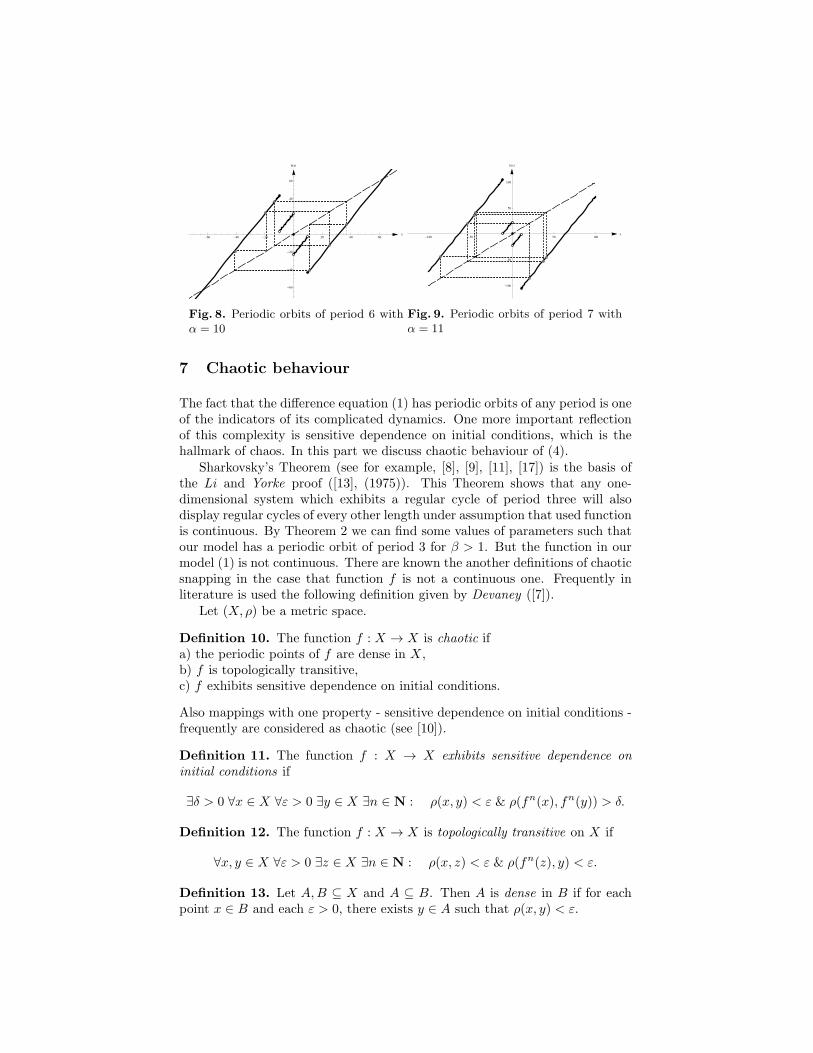
-60 -40 -20 20 40 60
x
-60
-40
-20
20
40
60
hHxL
Fig. 8. Periodic orbits of period 6 withα = 10
-100 -50 50 100
x
-100
-50
50
100
hHxL
Fig. 9. Periodic orbits of period 7 withα = 11
7 Chaotic behaviour
The fact that the difference equation (1) has periodic orbits of any period is oneof the indicators of its complicated dynamics. One more important reflectionof this complexity is sensitive dependence on initial conditions, which is thehallmark of chaos. In this part we discuss chaotic behaviour of (4).
Sharkovsky’s Theorem (see for example, [8], [9], [11], [17]) is the basis ofthe Li and Yorke proof ([13], (1975)). This Theorem shows that any one-dimensional system which exhibits a regular cycle of period three will alsodisplay regular cycles of every other length under assumption that used functionis continuous. By Theorem 2 we can find some values of parameters such thatour model has a periodic orbit of period 3 for β > 1. But the function in ourmodel (1) is not continuous. There are known the another definitions of chaoticsnapping in the case that function f is not a continuous one. Frequently inliterature is used the following definition given by Devaney ([7]).
Let (X, ρ) be a metric space.
Definition 10. The function f : X → X is chaotic ifa) the periodic points of f are dense in X,b) f is topologically transitive,c) f exhibits sensitive dependence on initial conditions.
Also mappings with one property - sensitive dependence on initial conditions -frequently are considered as chaotic (see [10]).
Definition 11. The function f : X → X exhibits sensitive dependence oninitial conditions if
∃δ > 0 ∀x ∈ X ∀ε > 0 ∃y ∈ X ∃n ∈ N : ρ(x, y) < ε & ρ(fn(x), fn(y)) > δ.
Definition 12. The function f : X → X is topologically transitive on X if
∀x, y ∈ X ∀ε > 0 ∃z ∈ X ∃n ∈ N : ρ(x, z) < ε & ρ(fn(z), y) < ε.
Definition 13. Let A,B ⊆ X and A ⊆ B. Then A is dense in B if for eachpoint x ∈ B and each ε > 0, there exists y ∈ A such that ρ(x, y) < ε.
66

In particular case if a = 0, then, for example, with parameters β = 2, b = 6,α = 3 in interval [0; 6] our function is a doubling map which is chaotic [1], [15],[16], [17]. This particular situation is shown in Fig.10 a).
In our case we use theorem from the book by Robinson [17].
Theorem 3. Assume that1) f is a function defined on a closed interval [a, b] ⊂ R with k discontinuities,2) f([a, b]) ⊂ [a, b],3) the map f is differentiable at all points x different from the discontinuitiespoints, with a derivative that satisfies |f ′(x)| > 1 at all these points, with xdifferent from the discontinuities points.Then f is a chaotic mapping.
-6 -4 -2 2 4 6
x
-6
-4
-2
2
4
6
hHxL
a)
-4 -2 2 4
x
-4
-2
2
4
hHxL
b)
Fig. 10. Chaotic functions
Therefore we can formulate a following theorem.
Theorem 4. There exists parameters β, α, b and a such that the function
h(x) =
βx− b, α ≤ x,βx− a, 0 < x < α,0, x = 0,βx+ a, −α < x < 0,βx+ b, x ≤ −α
is a chaotic mapping in some interval.
For example in case if bβ−1 = a = βα − a the interval is
[− bβ−1 ,
bβ−1
]. If
β = 3, a = 3, b = 6, α = 2 and the function h(x) is chaotic in the interval[−3, 3] (see Fig.10 b)).
References
1. K.T. Alligood and T.D. Sauer and J.A. Yorke. CHAOS. An Introduction to Dy-namical Systems. Springer-Verlag New York, Inc., 1997.
2. A. Anisimova and M. Avotina and I. Bula. Periodic Orbits of Single Neuron Modelswith Internal Decay Rate 0 < β ≤ 1. Mathematical Modelling and Analysis, 18,325–345, 2013.
67

3. A. Anisimova, M.Avotina, I.Bula. Periodic and Chaotic Orbits of a Neuron Model.Mathematical Modelling and Analysis, 20(1), 30–52 2015.
4. I.Bula, M.A.Radin. Periodic orbits of a neuron model with periodic internal decayrate. Applied Mathematics and Computation, 266, 293–303, 2015.
5. I.Bula, M. A.Radin, N.Wilkins. Neuron model with a period three internal decayrate. Electronic Journal of Qualitative Theory of Differential Equations, 46, 1–19,2017.
6. Y. Chen. All Solutions of a Class of Difference Equations are Truncated Periodic.Applied Mathematics Letters, 15, 975–979, 2002.
7. R. Devaney. An Introduction to Chaotic Dynamical Systems. Sec.ed., Addison-Wesley, 1989.
8. S.N. Elaydi. An Introduction to Difference Equations. Sec.ed., Springer-Verlag NewYork, Inc., 1999.
9. S.N. Elaydi. Discrete Chaos. With Applications in Science and Engineering. Sec.ed.,Chapman&Hall, CRC, 2008.
10. D. Gulick. Encounters with Chaos. McGraw-Hill, 1992.11. R.A. Holmgren. A First Course in Discrete Dynamical Systems, 2nd edn. Springer-
Verlag New York, 1996.12. M.R.S. Kulenovic and O. Merino. Discrete Dynamical Systems and Difference
Equations with Mathematica. Chapman&Hall, CRC, 2002.13. T.Y. Li and J.A. Yorke. Period Three Implies Chaos. The American Mathematical
Monthly, 82, 985–992, 1975.14. R.M. May. Simple mathematical models with very complicated dynamics. Nature,
261, 459–467, 1976.15. H.O. Peitgen and H.Juergen and D.Saupe. Chaos and Fractals. New Frontiers of
Science. Sec.ed., Springer-Verlag New York, Inc., 2004.16. H.O. Peitgen and H.Juergen and D.Saupe. Chaos - Bausteine der Ordnung.
Springer-Verlag Klett-Cotta, 1994.17. R.C. Robinson. An Introduction to Dynamical Systems. Continuous and Discrete.
Pearson Education, 2004.18. Z. Yuan and L. Huang and Y. Chen. Convergence and Periodicity of Solutions for
a Discrete-Time Network Model of Two Neurons. Mathematical and ComputerModelling, 45, 941–950, 2002.
19. Z. Wei and L. Huang and Y. Meng. Unboundedness and periodicity of solutions fora discrete-time network model of three neurons. Applied Mathematical Modelling,32, 1463–1474, 2008.
20. J. Wu. Introduction to Neural Dynamics and Signal Transmission Delay. DeGruyter, Berlin, 2001.
21. Z. Zhou. Periodic Orbits on Discrete Dynamical Systems. Computers and Math-ematics with Applications, 45, 1155–1161, 2003.
22. Z. Zhou and J. Wu. Stable Periodic Orbits in Nonlinear Discrete-Time Neuralnetworks with Delayed Feedback. Computers and Mathematics with Applications,45, 935–942, 2003.
23. H. Zhu and L. Huang. Dynamics of a Class of Nonlinear Discrete-Time neuralNetworks. Computers and Mathematics with Applications, 48, 85–94, 2004.
68
M-theory as a dynamical system generator
M. Axenides,1 E. Floratos,1,2 D. Katsinis,1,2 G. Linardopoulos1,2
1 Institute of Nuclear and Particle Physics, N.C.S.R. ”Demokritos”153 10, Agia Paraskevi, Greece.
2 Department of Nuclear and Particle Physics, Faculty of Physics, National andKapodistrian University of Athens. 157 84 Athens, Greece.
E-mails: [email protected], [email protected],[email protected], [email protected].
Abstract. We review our recent work on ellipsoidal M2-brane solutions in the large-N limit of the BMN matrix model. These bosonic finite-energy membranes live insideso (3) × so (6) symmetric plane-wave spacetimes and correspond to local extrema ofthe energy functional. They are static in so (3) and stationary in so (6). Chaos ap-pears at the level of radial stability analysis through the explicitly derived spectrum ofeigenvalues. The angular perturbation analysis is suggestive of the presence of weakturbulence instabilities that propagate from low to high orders in perturbation theory.
Keywords: Dynamical systems, chaos, M-theory, BMN matrix model, relativisticmembranes.
1 Introduction
M-theory By the end of the first superstring revolution (1984-1994), five seem-ingly different 10-dimensional superstring theories had emerged:
Types I, II (IIA, IIB), Heterotic (so(32), E8 × E8).
During the subsequent second superstring revolution (1994-2003), it was foundthat the 5 superstring theories are connected via a web of dualities (T-duality,S-duality, U-duality, mirror symmetry). What is more, it was realized thatthe five 10-dimensional superstring theories were just limiting cases of an 11-dimensional theory. This theory was called ”M-theory”; it is obtained in thestrong-coupling limit (gs → ∞) of IIA superstring theory. The letter ”M”stands for ”magic, mystery and matrix” according to one of its founders, E.Witten [1]. Others have associated the letter ”M” with ”membranes” [2].
Relativistic membranes The idea behind the theory of relativistic membranesis simple: replace 1-dimensional lines (strings) with 2-dimensional surfaces(membranes), much like lines/strings replace 0-dimensional points/particles inthe passage from quantum field theory to string theory. Like point particles
13thCHAOS Conference Proceedings, 9 - 12 June 2020, Florence, ItalyC. H. Skiadas (Ed)
© 2020 ISAST
69

2 Axenides et al
and strings, membranes are Poincare invariant objects that can be supersym-metrized. It has been proven that supermembranes can only be defined consis-tently in 11 spacetime dimensions. Higher-dimensional extended supersymmet-ric objects (Mp-branes) can be defined in an analogous fashion. Nonetheless,there are reasons to believe that supermembranes (or ”M2-branes”) are thefundamental objects of the 11-dimensional M-theory, just like strings are thefundamental objects of 10-dimensional string theory.
Matrix models According to the matrix theory conjecture of Banks, Fischler,Shenker and Susskind (BFSS) [3], a theory of matrix-discretized supermem-branes provides a realization of M-theory in flat spacetime. In the language ofmatrix models, membranes are fuzzy objects that are represented by N × Nmatrices. In the limit of very large matrix dimensions (N →∞), these matrixmodels are known to reduce to supermembrane theories.
In 2002, Berenstein, Maldacena and Nastase (BMN) [4] proposed a refor-mulation of the BFSS matrix model on a particular type of a background thatconsists of a weakly curved spacetime that is known as a plane-wave, supportedby a constant (4-form) field strength:
ds2 =−2dx+dx− −
µ2
9
3∑i=1
xixi +µ2
36
6∑j=1
yjyj
dx+dx+ +
3∑i=1
dxidxi+
+
6∑j=1
dyjdyj , F123+ = µ. (1)
Briefly, the BMN matrix model is a deformation of the BFSS matrix model bymass terms and a flux (aka Myers) term. In the large-N limit it is again known[5] that the BMN matrix model reduces to a theory of supermembranes in the11-dimensional plane-wave background (1). Interestingly, M(atrix) theory hasquite recently been applied to the study of chaotic phenomena that take placeon the horizons of black holes.
Black holes Black holes (BHs) are regions of spacetime where the force of grav-ity is so strong that nothing (not even light) can escape. The 2-dimensionalsurface beyond which it is (classically) impossible for matter or information toescape the gravitational pull of a BH is known as the BH’s event horizon. In1974 Stephen Hawking predicted that it is (quantum-mechanically) possible forBHs to emit thermal radiation and thus slowly evaporate. Because Hawking’sradiation is purely thermal, all the information that is stored in BHs seems toget lost.
To resolve the ensuing BH information paradox we ultimately need to un-derstand the mechanisms with which information is being stored and processedin BHs. One such mechanism is known as fast scrambling or ultra-fast thermal-ization [6]. More generally, it is widely believed that chaotic phenomena are adominant feature of BH horizons. Because it is inherently nonlocal, M(atrix)theory turns out to be a valuable tool in the study of information processingby BHs. More precisely, M(atrix) theory can be used to model the dynamicsof the microscopic degrees of freedom that are present on BH horizons [7,8].
70

M-theory as a dynamical system 3
2 General setup
Our starting point is the Hamiltonian of a bosonic relativistic membrane in the11-dimensional maximally supersymmetric plane-wave background (1). TheHamiltonian reads, in the so-called light-cone gauge x+ = τ [5]:
H =T
2
∫d2σ
[π2i +
1
2xi, xj2 +
1
2yi, yj2 + xi, yj2 +
µ2x2
9+µ2y2
36−
−µ3εijk xi, xjxk
]. (2)
From now on the indices of the coordinates xi will implicitly be taken to runfrom 1 to 3, while those of the coordinates yj will run from 1 to 6.1 In (2) Tstands for the membrane tension and
π2i ≡
3∑i=1
xixi +
6∑j=1
yj yj , x2 ≡3∑i=1
xixi, y2 ≡6∑j=1
yjyj . (3)
The definition of the Poisson bracket f, g that we will be using is
f , g ≡ εrs√w (σ)
∂rf ∂sg =1√w (σ)
(∂1f ∂2g − ∂2f ∂1g) , (4)
where d2σ =√w (σ) dσ1 dσ2 is the spatial volume element of the worldvolume
and εrs is the 2-dimensional Levi-Civita symbol. In a flat worldvolume it’sw (σ) = 1 and the usual definition of the Poisson bracket is retrieved.
The Lagrangian equations of motion for the spatial coordinates x and ycorresponding to the Hamiltonian (2) are:
xi = xi, xj , xj+ xi, yj , yj −µ2
9xi +
µ
2εijk xj , xk (5)
yi = yi, yj , yj+ yi, xj , xj −µ2
36yi. (6)
The coordinates x and y can also be shown to obey the Gauss law constraint:
3∑i=1
xi, xi+
6∑j=1
yj , yj = 0. (7)
3 The spherical ansatz
Let us make the following ansatz for the spatial coordinates x and y [9,10]:
xi ≡ x1i = x1i (τ) e1 (σ) , i = 1, . . . , q1 (8)
xq1+j ≡ x2j = x2j (τ) e2 (σ) , j = 1, . . . , q2 & q1 + q2 + q3 = 3 (9)
xq1+q2+k ≡ x3k = x3k (τ) e3 (σ) , k = 1, . . . , q3 (10)
1 Note also that there’s no distinction between upper and lower indices, so that thesewill be henceforth used interchangeably.
71

4 Axenides et al
and
yi ≡ y1i = y1i (τ) e1 (σ) , i = 1, . . . , s1 (11)
ys1+j ≡ y2j = y2j (τ) e2 (σ) , j = 1, . . . , s2 & s1 + s2 + s3 = 6 (12)
ys1+s2+k ≡ y3k = y3k (τ) e3 (σ) , k = 1, . . . , s3. (13)
The ansatz (8)–(13) splits the coordinates x and y into three groups
xai = xai (τ) ea & ybj = ybj (τ) eb, (14)
where i = 1, . . . , qa, j = 1, . . . , sb, a, b = 1, 2, 3. Going over to sphericalcoordinates, (σ1, σ2)→ (θ, φ), we define:2
(e1, e2, e3) = (cosφ sin θ, sinφ sin θ, cos θ), φ ∈ [0, 2π), θ ∈ [0, π] (16)
ei, ej = εijk ek,
∫ei ej d
2σ =4π
3δij . (17)
Note that the Gauss law constraint (7) is automatically satisfied by the ansatz(8)–(13). Now consider the following solutions:
x1 (τ) = eΩx1τ · x10, x2 (τ) = eΩx2τ · x20, x3 (τ) = eΩx3τ · x30 (18)
y1 (τ) = eΩy1τ · y10, y2 (τ) = eΩy2τ · y20, y3 (τ) = eΩy3τ · y30. (19)
As in the case of flat space (worked out in [11]) it can be shown that the radii
r2x1 ≡ x2
1 =
q1∑i=1
x10ix10i, r2x2 ≡ x2
2 =
q2∑j=1
x20j x20j , r2x3 ≡ x2
3 =
q3∑k=1
x30kx30k (20)
r2y1 ≡ y2
1 =
s1∑i=1
y10iy10i, r2y2 ≡ y2
2 =
s2∑j=1
y20j y20j , r2y3 ≡ y2
3 =
23∑k=1
y30ky30k (21)
of the ansatz (18)–(19) can be determined (for all the antisymmetric matricesΩx1, Ωx2, Ωx3, Ωy1, Ωy2, Ωy3) in terms of the conserved angular momenta
(`x1)ij ≡ ˙x1ix1j − x1i˙x1j , (`y1)ij ≡ ˙y1iy1j − y1i
˙y1j (22)
(`x2)ij ≡ ˙x2ix2j − x2i˙x2j , (`y2)ij ≡ ˙y2iy2j − y2i
˙y2j (23)
(`x3)ij ≡ ˙x3ix3j − x3i˙x3j , (`y3)ij ≡ ˙y3iy3j − y3i
˙y3j , (24)
by minimizing the corresponding effective potential of the membrane. This iscompletely equivalent to plugging the ansatz (18)–(19) into the equations ofmotion (5)–(6) and determining the relation between the radii rx1, rx2, rx3,ry1, ry2, ry3 and the components of the matrices Ωx1, Ωx2, Ωx3, Ωy1, Ωy2, Ωy3
(which in turn always combine to form the conserved angular momenta `x1,`x2, `x3, `y1, `y2, `y3).
2 We use the volume element in (θ, φ) space which implies that√w (σ) = sin θ should
be used in the definition (4) of the Poisson bracket. For alternative parametrizationssuch as
(e1, e2, e3) = (cn (φ|m) sn (θ|n) , sn (φ|m) sn (θ|n) , sn (θ|n)), (15)
where φ ∈ [0, 4K (m)) and θ ∈ [0, 2K (n)], the corresponding volume element is√w (σ) = sn (θ|n) dn (θ|n) dn (φ|m).
72

M-theory as a dynamical system 5
4 Effective potentials
The energy of the membrane (2) becomes:
E =2πT
3
[˙x21 + ˙x2
2 + ˙x23 + ˙y2
1 + ˙y22 + ˙y2
3 + x21x
22 + x2
2x23 + x2
3x21 + y2
1 y22 + y2
2 y23+
+y23 y
21 + x2
1
(y2
2 + y23
)+ x2
2
(y2
3 + y21
)+ x2
3
(y2
1 + y22
)+µ2
9x2+
+µ2
36y2 − 2µ εijk x1ix2j x3k
]. (25)
We now proceed to the following decomposition of the coordinates:
˙x21 ≡ ˙x1i
˙x1i = r2x1 +
`2x1
r2x1
, ˙y21 ≡ ˙y1j
˙y1j = r2y1 +
`2y1
r2y1
(26)
˙x22 ≡ ˙x2i
˙x2i = r2x2 +
`2x2
r2x2
, ˙y22 ≡ ˙y2j
˙y2j = r2y2 +
`2y2
r2y2
(27)
˙x23 ≡ ˙x3i
˙x3i = r2x3 +
`2x3
r2x3
, ˙y23 ≡ ˙y3j
˙y3j = r2y3 +
`2y3
r2y3
. (28)
Plugging (20)–(21) and (26)–(28) into (25), we find that the energy of themembrane becomes
E =2πT
3
[r2x1 + r2
x2 + r2x3 + r2
y1 + r2y2 + r2
y3 +`2x1
r2x1
+`2x2
r2x2
+`2x3
r2x3
+`2y1
r2y1
+`2y2
r2y2
+
+`2y3
r2y3
+ r2x1r
2x2 + r2
x2r2x3 + r2
x3r2x1 + r2
y1r2y2 + r2
y2r2y3 + r2
y3r2y1+
+r2x1
(r2y2 + r2
y3
)+ r2
x2
(r2y3 + r2
y1
)+ r2
x3
(r2y1 + r2
y2
)+µ2
9(r2x1+
+r2x2 + r2
x3) +µ2
36
(r2y1 + r2
y2 + r2y3
)− 2µ εijkx1ix2j x3k
], (29)
so that the corresponding effective potential reads
Veff =2πT
3
[`2x1
r2x1
+`2x2
r2x2
+`2x3
r2x3
+`2y1
r2y1
+`2y2
r2y2
+`2y3
r2y3
+ r2x1r
2x2 + r2
x2r2x3 + r2
x3r2x1+
+r2y1r
2y2 + r2
y2r2y3 + r2
y3r2y1 + r2
x1
(r2y2 + r2
y3
)+ r2
x2
(r2y3 + r2
y1
)+
+r2x3
(r2y1 + r2
y2
)+µ2
9
(r2x1 + r2
x2 + r2x3
)+µ2
36
(r2y1 + r2
y2 + r2y3
)−
−2µ εijkx1ix2j x3k
]. (30)
The above potential (30) contains four different kinds of terms, either re-pulsive or attractive: (1) kinetic/angular momentum terms (repulsive), (2)
73

6 Axenides et al
quartic interaction terms (attractive), (3) mass terms (attractive), and (4) acubic Myers flux term (repulsive). The last two kinds of terms (i.e. the massterms (3) and the Myers term (4)) are µ-dependent and so they drop out in theµ → 0 limit (flat space) that was studied in [11]. In both cases (either µ = 0or µ 6= 0), it is the equilibration of attractive and repulsive forces that deter-mines the extrema of the potential. The two extra repulsive/attractive termsfor µ 6= 0 (induced by the plane-wave background) increase the complexity ofthe resulting dynamical system, as it will become apparent below.
There are three ways to distribute the so (3) coordinates xi (i = 1, 2, 3) intothe three groups that are specified by the units ei in (16), so that we can gener-ally distinguish three main types of membrane configurations. The first two ofthem (labelled types I and II below) describe rotating membranes (tops) thatare point-like (collapsed) in one or two so (3) directions and have a vanishingMyers flux term. The third type (III) is probably the most interesting one asit contains all four kinds of repulsive and attractive terms that we describedabove and extends into the full geometric background of so (3)× so (6). Let usnow introduce these three types of configurations.
4.1 Type I: q1 = 3, q2 = q3 = 0
For q1 = 3, q2 = q3 = 0 we have
rx ≡ rx1, rx2 = rx3 = 0 & `x ≡ `x1, `x2 = `x3 = 0 (31)
and the flux term vanishes. The effective potential (30) of the membranebecomes:
Veff =2πT
3
[`2xr2x
+`2y1
r2y1
+`2y2
r2y2
+`2y3
r2y3
+ r2y1r
2y2 + r2
y2r2y3 + r2
y3r2y1 + r2
x
(r2y2 + r2
y3
)+µ2r2
x
9+µ2
36
(r2y1 + r2
y2 + r2y3
) ]. (32)
Apart from the completely symmetric (single-radius) configuration r = rx =ry1 = ry2 = ry3, ` = `x = `y1 = `y2 = `y3, the radii and the momenta of theeffective potential (32) may be grouped into 5 different axially symmetric (2-radii) configurations and 4 more configurations with 3 different radii. Each ofthese potentials possesses a local minimum that corresponds to a stationary topsolution with time-independent radius and nonzero total angular momentum.There are no static solutions (i.e. having constant radius and zero angularmomentum) in this case.
4.2 Type II: q1 = 2, q2 = 1, q3 = 0
For q1 = 2, q2 = 1 and q3 = 0,
rx3 = 0 & `x2 = `x3 = 0 (33)
74

M-theory as a dynamical system 7
and the flux term vanishes again. The effective potential (30) becomes:
Veff =2πT
3
[`2x1
r2x1
+`2y1
r2y1
+`2y2
r2y2
+`2y3
r2y3
+ r2x1r
2x2 + r2
y1r2y2 + r2
y2r2y3 + r2
y3r2y1+
+r2x1
(r2y2 + r2
y3
)+ r2
x2
(r2y3 + r2
y1
)+µ2
9
(r2x1 + r2
x2
)+
+µ2
36
(r2y1 + r2
y2 + r2y3
) ]. (34)
Although again this case does not lead to any static configuration (with con-stant radius and zero angular momentum), we may construct one single-radius(r = rx1 = rx2 = ry1 = ry2 = ry3, ` = `x1 = `y1 = `y2 = `y3) solution, 13axially symmetric (2-radii) tops and 21 tops with 3 different radii.
For example let us consider a type II configuration with all the so (6) vari-ables set equal to zero:
x1 = x (τ) · e1, x2 = y (τ) · e1, x3 = z (τ) · e2, yi = 0, i = 1, . . . , 6, (35)
where the time-dependent part has the form (18). In this case the effectivepotential (34) becomes:
Veff =2πT
3
[`2
x2 + y2+(x2 + y2
)z2 +
µ2
9
(x2 + y2 + z2
) ], (36)
after setting `x1 = ` for simplicity. The corresponding extremisation condition∇Veff = 0 implies
x z2 +µ2x
9− x `2
(x2 + y2)2 = y z2 +
µ2y
9− y `2
(x2 + y2)2 = z
(x2 + y2
)+µ2z
9= 0,
which is solved by
x2 + y2 =3`
µ& z = 0. (37)
Complying with (18), we can choose e.g.:
x (τ) =
√3`
µcos
µ τ
3, y (τ) =
√3`
µsin
µ τ
3, z (τ) = 0. (38)
Equivalently we could have directly plugged (35) into the equations of mo-tion (5)–(6):
x · e1 = −x z2 · e1 −µ2x
9· e1 + µ y z · e3 (39)
y · e1 = −y z2 · e1 −µ2y
9· e1 + µx z · e3 (40)
z · e2 = −z(x2 + y2
)· e2 −
µ2z
9· e2. (41)
It is easily seen that any solution of the type (18) will again satisfy (37).
75

8 Axenides et al
4.3 Type III: q1 = q2 = q3 = 1
For q1 = q2 = q3 = 1, we write:
x1 = rx1e1, x2 = rx2e2, x3 = rx3e3 & `x1 = `x2 = `x3 = 0. (42)
Note that rx1, rx2, rx3 are not radii anymore, but coordinates. The effectivepotential (30) of the membrane can be written as:
Veff =2πT
3
[`2y1
r2y1
+`2y2
r2y2
+`2y3
r2y3
+ r2x1r
2x2 + r2
x2r2x3 + r2
x3r2x1 + r2
y1r2y2 + r2
y2r2y3+
+r2y3r
2y1 + r2
x1
(r2y2 + r2
y3
)+ r2
x2
(r2y3 + r2
y1
)+ r2
x3
(r2y1 + r2
y2
)+
+µ2
9
(r2x1 + r2
x2 + r2x3
)+µ2
36
(r2y1 + r2
y2 + r2y3
)− 2µrx1rx2rx3
]. (43)
By combining the various radii (along with the corresponding angular mo-menta) into groups of one, two or three, we obtain 30 different top configu-rations, one of which corresponds to a completely symmetric top, 9 to axiallysymmetric (2-radii) tops and 10 to tops that have 3 different radii.
5 Simple type III solutions
The so (3)× so (3)× so (3) ⊂ so (3)× so (6) invariant ansatz
xi = ui (τ) ei, yj = vj (τ) ej , yj+3 = wj (τ) ej , i, j = 1, 2, 3 (44)
was studied in [12]. The ansatz (44) is obviously of the form (42) (type III)and it describes rotating and pulsating membranes of spherical topology. Thecorresponding Hamiltonian
H =2πT
3
(p2u + p2
v + p2w
)+ U, (45)
is obtained by integrating out the worldvolume coordinates θ and φ. Thepotential energy U reads
U =2πT
3
[u2
1u22 + u2
2u23 + u2
3u21 + r2
1 r22 + r2
2 r23 + r2
3 r21 + u2
1
(r22 + r2
3
)+
+u22
(r23 + r2
1
)+ u2
3
(r21 + r2
2
)+µ2
9
(u2
1 + u22 + u2
3
)+
+µ2
36
(r21 + r2
2 + r23
)− 2µu1u2u3
], r2
j ≡ v2j + w2
j , j = 1, 2, 3. (46)
The manifest so (2)×so (2)×so (2) symmetry of the Hamiltonian (45)–(46)with respect to the so (6) coordinates vi and wi implies that any solution ofthe equations of motion preserves three so (2) angular momenta `i (i = 1, 2, 3).
76

M-theory as a dynamical system 9
The kinetic terms of the Hamiltonian (45) can be expressed in terms of theconserved angular momenta `i as
p2v + p2
w =
3∑i=1
(˙r2i +
`2ir2i
), (47)
leading to the effective potential
Veff = U +2πT
3
(`21r21
+`22r22
+`23r23
). (48)
5.1 The so (3) symmetric membrane
Let us now consider the simplest possible subsystem of (44) where the so (6)variables vi and wi are set to zero [12]:
vi = wi = 0, i = 1, 2, 3. (49)
Scaling out the mass parameter µ by setting
t = µτ, ui = µui (50)
leads to the form
Veff =2πTµ4
3
[u2
1u22 + u2
2u23 + u2
1u23 +
1
9
(u2
1 + u22 + u2
3
)− 2u1u2u3
](51)
of the membrane effective potential (48) and the Hamilton equations of motion,
u1 = p1, p1 = −[u1
(u2
2 + u23
)+u1
9− u2u3
](52)
u2 = p2, p2 = −[u2
(u2
3 + u21
)+u2
9− u3u1
](53)
u3 = p3, p3 = −[u3
(u2
1 + u22
)+u3
9− u1u2
]. (54)
The effective potential (51) is a particular instance of the generalized 3-dimensionalHenon-Heiles potential that was introduced in [13],
VHH =1
2
(u2
1 + u22 + u2
3
)+K3 u1u2u3 +K0
(u2
1 + u22 + u2
3
)2+
+K4
(u4
1 + u42 + u4
3
), (55)
with K3 = −9, K0 = −K4 = 9/4. The critical points of the effective potential(51) are:
u0 = 0, u1/6 =1
6· (1, 1, 1) , u1/3 =
1
3· (1, 1, 1) . (56)
6 more critical points can be obtained by flipping the sign of exactly two ui’s.This is consistent with the manifest tetrahedral (Td) symmetry of the potential(51). The extrema u0 (point-like membrane) and u1/3 (Myers dielectric sphere)are global degenerate minima of the potential while u1/6 is a saddle point:
Veff (0) = Veff
(1
3
)= 0, Veff
(1
6
)=
2πTµ4
64. (57)
77

10 Axenides et al
Radial spectrum [12] By radially perturbing the 9 critical points u0i in (56) as
ui = u0i + δui (t) , δui (t) =
6∑k=1
ckeiλtξik, (58)
we may confirm the above conclusion by examining the corresponding Hessianmatrix. It turns out that u0 and u1/3 are global minima (positive-definiteHessian) and u1/6 is a saddle point (indefinite Hessian). These results aresummarized in the following table 1.
critical point eigenvalues λ2 (#) stability
u019
(3) , 136
(6) center (S)
u1/6 − 118
(1) , 518
(2) , 112
(6) saddle point
u1/319
(1) , 49
(2) , 14
(6) center (S)
Table 1. Radial spectrum of the so (3) symmetric membrane.
Angular spectrum [14] We may also perform more general (angular/multipole)perturbations of the following form:
xi (t) = x0i + δxi (t) , i = 1, 2, 3, (59)
where δxi is expanded in spherical harmonics Yjm (θ, φ) as
xi (t) = µui (t) ei, x0i ≡ µu0
i ei, δxi (t) = µ ·∞∑j=1
j∑m=−j
ηjmi (t)Yjm (θ, φ) . (60)
For the critical points u0, u1/6, u1/3 we find the eigenvalues [12]:
u0 : λ2P = λ2
± =1
9, λ2
θ =1
36(61)
u1/6 : λ2P = 0, λ2
+ =1
36(j + 1) (j + 4) , λ2
− =j (j − 3)
36,
λ2θ =
1
36
(j2 + j + 1
)(62)
u1/3 : λ2P = 0, λ2
+ =1
36(j + 1)
2, λ2− =
j2
9, λ2
θ =1
36(2j + 1)
2, (63)
with multiplicities dP = 2j + 1, d+ = 2j + 3, d− = 2j − 1 and dθ = 6 (2j + 1),respectively.
The critical point u0 (point-like membrane) is obviously stable. u1/3 hasa zero mode of degeneracy 2dP while all its other eigenvalues are stable forj = 1, 2, . . . u1/6 has one 2dP -degenerate zero mode for every j and a 10-folddegenerate zero mode for j = 3. It is unstable for j = 1 (2-fold degenerate) andj = 2 (6-fold degenerate). The above results were first obtained by [5] from thematrix model. In the flat-space limit (µ→ 0), we recover the results of [15,16].
78

M-theory as a dynamical system 11
5.2 The so (3) × so (3) × so (3) symmetric membrane
Similar perturbative analyses can be carried out in the so (3)× so (6) sector. Asolution of the corresponding equations of motion is given by
u0i = u0, v0
j (t) = v0 cos (ωt+ ϕj) , w0j (t) ≡ v0
j+3 (t) = v0 sin (ωt+ ϕk) , (64)
where (u0, v0) are the critical points of the axially symmetric potential
V ≡ Veff
2πTµ4= u4+2u2v2 + v4 +
u2
9+v2
36− 2u3
3+`2
v2(65)
and `µ3 ≡ `1 = `2 = `3. It can be proven that the critical points (u0, v0) alwayslie within the interval:
1
6≤ u0 ≤
1
3& 0 ≤ v0 ≤
1
12. (66)
Radial spectrum [12] To obtain the radial spectrum we set
ui = u0i + δui (t) , vi = v0
i (t) + δv′i (t) , wi = w0i (t) + δw′i (t) , (67)
finding six zero eigenvalues and four nonzero ones (quadruply and doubly de-generate):
λ21± =
5u0
2− 1
9±√
1
92− u0
9− 5u2
0
12+ 4u3
0 (68)
λ22± =
5u0
2− 5
18±√
52
182− 35u0
18+
163u20
12− 20u3
0. (69)
The plots of these eigenvalues can be found in the following figure 1.
u0 =1
6u0 =
1
3ucrit
0.10 0.15 0.20 0.25 0.30 0.35u0
-0.2
0.2
0.4
0.6
0.8
1.0
1.2
λ2(u0)
Fig. 1. Radial spectrum of the so (3)× so (6) symmetric membrane.
Angular spectrum [14] Going further, we again set out to perform angular/multipoleperturbations of the form:
xi = x0i + δxi, i = 1, 2, 3 & yk = y0
k + δyk, k = 1, . . . , 6, (70)
79

12 Axenides et al
where the δxi, δyk are expanded around the classical solution,
x0i = µu0ei, i = 1, 2, 3, y0
i = µv0i (t) e1, i = 1, 2 (71)
y0k = µv0
k (t) e2, k = 3, 4 (72)
y0l = µv0
l (t) e3, l = 5, 6, (73)
in spherical harmonics Yjm (θ, φ):
δxi = µ ·∑j,m
ηjmi (τ)Yjm (θ, φ) , δyk = µ ·∑j,m
εjmk (τ)Yjm (θ, φ) (74)
δyl = µ ·∑j,m
ζjml (τ)Yjm (θ, φ) , (75)
for i = 1, 2, 3, k = 1, 3, 5, l = 2, 4, 6. We find that one of the eigenvalues alwaysvanishes, two others are given by the following analytic expression
λ2P =
1
2
(j2 + j + 2
)u0−
1
18
(1 + j (j + 1)±
±3√
144 (j2 + j − 2)u30 − 12 (j2 + j − 14)u2
0 − 24u0 + 1
), (76)
while 6 more eigenvalues λ± are also known in closed forms but are too compli-cated to be included here. The corresponding multiplicities of the eigenvaluesare dP = 2j + 1, d+ = 2j + 3, d− = 2j − 1. For j = 1 four eigenvalues vanish,while two others coincide with the eigenvalues (68)–(69) that were found fromradial perturbations:
λ2P = 4u0 +
1
3, λ2
+ =5u0
2− 1
9±√
1
92− u0
9− 5u2
0
12+ 4u3
0 (77)
λ2− =
5u0
2− 5
18±√
52
182− 35u0
18+
163u20
12− 20u3
0. (78)
For j = 2 there’s one zero eigenvalue while λP > 0. We can also plot the j = 2eigenvalues of λ± (figure 2):
0.10 0.15 0.20 0.25 0.30 0.35u0
0.5
1.0
1.5
2.0
λ2(u0)
0.10 0.15 0.20 0.25 0.30 0.35u0
-0.5
0.5
1.0
1.5
2.0
λ2(u0)
Fig. 2. λ2± for j = 2 as a function of u0.
• The squared nonzero j = 1 eigenvalues are all positive/stable in the interval(66), except λ2
−(−) which is positive/stable only for ucrit < u0 < 1/3, where
ucrit ≡ 160
(11 +
√21).
80

M-theory as a dynamical system 13
• For j = 2, the λP , λ+ and one of the λ− squared eigenvalues are pos-itive/stable in the interval (66). The remaining λ2
− eigenvalue is nega-tive/unstable in the interval 1
6 ≤ u0 ≤ 0.207245 < ucrit.
• For j ≥ 3 all the squared eigenvalues are non-negative inside the interval(66) and so the system is stable .
Here’s a summary of the angular/multipole spectrum (table 2):
eigenvalues j = 1 j = 2 j ≥ 3 degeneracy
λ2P 0, 0,+ 0,+,+ 0,+,+ dP = 2j + 1
λ2+ 0,+,+ +,+,+ +,+,+ d+ = 2j + 3
λ2− 0,+, 0,± +,+, 0,± +,+,+ d− = 2j − 1(positive for
u0 > ucrit
) ( positive foru0 > 0.207245
)Table 2. Angular spectrum of the so (3)× so (6) symmetric membrane.
Higher-order perturbations [17] Beyond linearized perturbation theory (alwaysinside the interval (66)), we anticipate a cascade of instabilities that originatesfrom the j = 1, 2 multipoles and propagates towards all higher modes (j =3, 4, . . .). The perturbative expansion becomes
xi =
∞∑n=0
εnδxni = x0i +
∞∑n=1
εnδxni , i = 1, 2, 3 (79)
yi =
∞∑n=0
εnδyni = y0i +
∞∑n=1
εnδyni , i = 1, . . . , 6. (80)
It follows that any given mode j at any given order n in perturbation theorycouples to all the modes of the previous orders 1, . . . , n−1 through an effectiveforcing term that emerges in the corresponding system of fluctuation equations.The perturbations are expanded in spherical harmonics as
δxni = µ ·∑j,m
ηnjmi (τ)Yjm (θ, φ) , ηnjmi (0) = 0, i = 1, 2, 3 (81)
δyni = µ ·∑j,m
θnjmi (τ)Yjm (θ, φ) , θnjmi (0) = 0, i = 1, . . . , 6. (82)
For example it can be shown that the (n = 1, j = 1, 2) instabilities we foundabove couple to every mode (j = 1, 2, . . .) of the second order (n = 2) inperturbation theory.
81

14 Axenides et al
6 Acknowledgements
The authors would like to thank Christos Skiadas for the invitation to partic-ipate to the 13th CHAOS conference. This research is funded in the contextof the project ”Chaotic dynamics and black holes in BMN theory” E-12386(MIS 5047794) under the call for proposals ”Supporting researchers with anemphasis on young researchers—Cycle B” (EDULLL 103). The project is co-financed by Greece and the European Union (European Social Fund—ESF) bythe Operational Programme Human Resources Development, Education andLifelong Learning 2014-2020.
References
1. E. Witten, Magic, mystery, and matrix, Not. Amer. Math. Soc. 45 (1998) 1124.2. M. J. Duff, Benchmarks on the brane, hep-th/0407175.3. T. Banks, W. Fischler, S. H. Shenker, and L. Susskind, M-theory as a matrix
model: A conjecture, Phys. Rev. D55 (1997) 5112, [hep-th/9610043].4. D. Berenstein, J. Maldacena, and H. Nastase, Strings in flat space and pp waves
from N = 4 super Yang-Mills, JHEP 04 (2002) 013, [hep-th/0202021].5. K. Dasgupta, M. M. Sheikh-Jabbari, and M. Van Raamsdonk, Matrix perturbation
theory for M-theory on a pp-wave, JHEP 05 (2002) 56, [hep-th/0205185].6. Y. Sekino and L. Susskind, Fast scramblers, JHEP 10 (2008) 065,
[arXiv:0808.2096].7. G. Gur-Ari, M. Hanada, and S. H. Shenker, Chaos in classical D0-brane
mechanics, JHEP 02 (2016) 091, [arXiv:1512.00019].8. Y. Asano, D. Kawai, and K. Yoshida, Chaos in the BMN matrix model, JHEP 06
(2015) 191, [arXiv:1503.04594].9. P. A. Collins and R. W. Tucker, Classical and quantum mechanics of free
relativistic membranes, Nucl. Phys. B112 (1976) 150.10. T. Harmark and K. G. Savvidy, Ramond-Ramond field radiation from rotating
ellipsoidal membranes, Nucl. Phys. B585 (2000) 567, [hep-th/0002157].11. M. Axenides and E. Floratos, Euler top dynamics of Nambu-Goto p-branes,
JHEP 03 (2007) 093, [hep-th/0608017].12. M. Axenides, E. Floratos, and G. Linardopoulos, M2-brane dynamics in the
classical limit of the BMN matrix model, Phys. Lett. B773 (2017) 265,[arXiv:1707.02878].
13. K. Efstathiou and D. Sadovskiı, Perturbations of the 1:1:1 Resonance withtetrahedral symmetry: a three degree of freedom analogue of the two degree offreedom Henon–Heiles Hamiltonian, Nonlinearity 17 (2004) 415.
14. M. Axenides, E. Floratos, and G. Linardopoulos, Multipole stability of spinningM2 branes in the classical limit of the BMN matrix model, Phys. Rev. D97(2018) 126019, [arXiv:1712.06544].
15. M. Axenides, E. G. Floratos, and L. Perivolaropoulos, Metastability of sphericalmembranes in supermembrane and matrix theory, JHEP 11 (2000) 020,[hep-th/0007198].
16. M. Axenides, E. G. Floratos, and L. Perivolaropoulos, Quadrupole instabilitiesof relativistic rotating membranes, Phys. Rev. D64 (2001) 107901,[hep-th/0105292].
17. M. Axenides, E. Floratos, D. Katsinis, and G. Linardopoulos to appear.
82
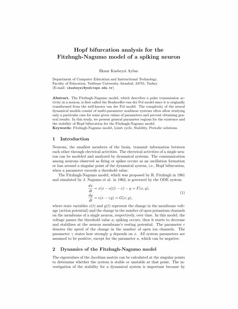
Hopf bifurcation analysis for theFitzhugh-Nagumo model of a spiking neuron
Ilknur Kusbeyzi Aybar
Department of Computer Education and Instructional Technology,Faculty of Education, Yeditepe University, Istanbul, 34755, Turkey(E-mail: [email protected])
Abstract. The Fitzhugh-Nagumo model, which describes a pulse transmission ac-tivity in a neuron, is first called the Bonhoeffer-van der Pol model since it is originallytransformed from the well-known van der Pol model. The complexity of the neuraldynamical models consist of multi-parameter nonlinear systems often allow studyingonly a particular case for some given values of parameters and prevent obtaining gen-eral results. In this study, we present general parameter regions for the existence andthe stability of Hopf bifurcation for the Fitzhugh-Nagumo model.Keywords: Fitzhugh-Nagumo model, Limit cycle, Stability, Periodic solutions.
1 Introduction
Neurons, the smallest members of the brain, transmit information betweeneach other through electrical activities. The electrical activities of a single neu-ron can be modeled and analyzed by dynamical systems. The communicationamong neurons observed as firing or spikes occurs as an oscillation formationor loss around a singular point of the dynamical system, i.e., Hopf bifurcation,when a parameter exceeds a threshold value.
The Fitzhugh-Nagumo model, which was proposed by R. Fitzhugh in 1961and simulated by J. Nagumo et al. in 1962, is governed by the ODE system
dx
dt= x(x− a)(1− x)− y = F (x, y),
dy
dt= ε(x− γy) = G(x, y),
(1)
where state variables x(t) and y(t) represent the change in the membrane volt-age (action potential) and the change in the number of open potassium channelson the membrane of a single neuron, respectively, over time. In this model, thevoltage passes the threshold value a; spiking occurs, then it starts to decreaseand stabilizes at the neuron membrane’s resting potential. The parameter εdenotes the speed of the change in the number of open ion channels. Theparameter γ states how strongly y depends on x. All system parameters areassumed to be positive, except for the parameter a, which can be negative.
2 Dynamics of the Fitzhugh-Nagumo model
The eigenvalues of the Jacobian matrix can be calculated at the singular pointsto determine whether the system is stable or unstable at that point. The in-vestigation of the stability for a dynamical system is important because by
83

this analysis it is then possible to know if all nearby trajectories approach thatpoint of singularity. If the real parts of the eigenvalues of the system’s Jaco-bian matrix are all negative at that point, the system is stable at this point ofsingularity; otherwise, it is unstable at that point[8]. If the real parts of theeigenvalues of the Jacobian matrix are a pair of pure imaginary values, thenthe phenomenon called Hopf bifurcation occurs at that point, which impliesthat at that point, the system is oscillating, that is, this singularity point isan oscillatory solution of the system. The limit cycle can be either stable orunstable, depending on the behaviour of the system. If all nearby trajectoriesapproach the limit cycle inward and outward, it is a stable limit cycle. In orderto determine the parameter regions for the existence of a stable limit cycle, wecalculate the first Lyapunov coefficient[4]. This study contributes to the com-prehension of the electrical activities of neurons by using the dynamical analysismethods since the spikes in the communication of neurons are mathematicallystable oscillatory solutions.
Proposition 1. System (1) has three singular points E0 = (0, 0),
E− = (1
2(1 + a−
√(a− 1)2 − 4
γ),
1
2γ(1 + a−
√(a− 1)2 − 4
γ)),
and
E+ = (1
2(1 + a+
√(a− 1)2 − 4
γ),
1
2γ(1 + a+
√(a− 1)2 − 4
γ)).
2.1 System dynamics at E0
At E0, the membrane voltage is zero, and the ion channels are all closed. Theeigenvalues of the Jacobian matrix at E0, which is at the resting potential, are
λ1,2 =1
2(−a− εγ ±
√(a− εγ)2 − 4ε). (2)
Proposition 2. The singular point E0 is a stable singular point when the sys-tem parameters a, ε, and γ are all positive or
−γε < a ≤ 0.
Theorem 1. According to the eigenvalues given in (2), system (1) exhibitsHopf bifurcation when
a < 0, ε > a2, a = −εγ. (3)
Proof. To investigate Hopf bifurcation at E0, we accept conditions (3) andcalculate the first Lyapunov coefficient at this point. We look for a Lyapunovfunction of the form
h(x, y) = αx2 + βxy + σy2 + h.o.t.
that satisfies
∂h
∂xF (x, y) +
∂h
∂yG(x, y) = g1(x2 + y2)2 + .... (4)
84

By solving (4) together with (1), we obtain
α =βε
2a
and
σ = − β
2εγ.
The quadratic form
4ασ − β2 = −4 +4
εγ2
is positive-definite when we choose β = 2 because of condition (3) which reducesto
ε > 0, 0 < γ <
√1
ε
in this case. We calculate the first Lyapunov coefficient as
g1 =6 + 2γ(εγ(1− 2εγ)− 2)
γ(3 + ε(2 + ε(3 + 4γ2))). (5)
Stable oscillations are indicated by a negative first Lyapunov coefficient. There-fore, we study the case g1 < 0 together with the conditions given in (3) and weconclude in the following Theorem.
Theorem 2. System (1) exhibits supercritical Hopf bifurcation when one ofthe following cases are satisfied:
(i)0 < γ < 1,1
4γ+
1
4
√−3(
(5γ − 8)
γ3) < ε <
1
γ2,
(ii)1 < γ ≤ 3
2,
1
4γ+
1
4
√−3(
5γ − 8
γ3) < ε <
1
γ2,
(iii)3
2< γ ≤ 8
5, 0 < ε <
1
4γ− 1
4
√−3(
5γ − 8
γ3),
(iv)3
2< γ ≤ 8
5,
1
4γ+
1
4
√−3(
5γ − 8
γ3) < ε <
1
γ2,
(v)γ >8
5, 0 < ε <
1
γ2.
(6)
Example 1. To demonstrate supercritical Hopf bifurcation at the origin wechoose the parameter set (a, ε, γ) = (−1.75, 0.5, 3.5). The eigenvalues of theJacobian matrix are λ1,2 = ±0.661438i. In Fig. 1, we illustrate that system(1) exhibits stable oscillatory regime, i.e. limit cycle. The trajectories outsideand inside approach to the limit cycle. In Fig. 1. (a) we have two initial points,one at the outside, and one at the inside of the limit cycle. This is clearly ob-vious since the first Lyapunov coefficient at this point is g1 = −0.0127119, aswe obtain by (5). In Fig. 1. (b), we choose ten different initial points.
85

-0.5 0 0.5
x
-1.5
-1
-0.5
0
0.5
1
y
(a)
-1 -0.5 0 0.5 1
x
-2
-1.5
-1
-0.5
0
0.5
1
1.5
y
(b)
Fig. 1. (a) The supercritical Hopf bifurcation of system (1) when (a, ε, γ) =(−1.75, 0.5, 3.5) around the origin. (b) The trajectories moving towards the limitcycle from ten different initial points outside.
2.2 System dynamics at E− and E+
In this section, we investigate the local dynamics of system (1) at the singu-lar point E−. However, same results are obtained for the singular point E+.First, we make assumption that the state variables and parameter values tobe real numbers to represent realistic values, which means that the expressionsin the root must be nonnegative. For this reason, we assume the square rootterms in the singular points are positive or at least zero. Hence, we begin ourinvestigation for Hopf bifurcation at E± by accepting the condition
∆ = (a− 1)2γ − 4 ≥ 0. (7)
The eigenvalues of the Jacobian matrix at E− are
λ1,2 =1
4γ(2−∆− 2εγ2 + (1 + a)
√γ∆
± 1
2
√−32εγ2(∆− (1 + a)
√γ∆) + 4(2−∆− 2εγ2 + (1 + a)
√γ∆)2).
(8)
86

Proposition 3. E− is a stable singular point under one of the following cases:
i.a < 1, ∆ = 0, ε >2−∆2γ2
,
ii.a < 1, ∆ > 0, ε >2−∆+
√γ∆(1 + a)
2γ2,
iii.a > 1, ∆ = 0, ε >2−∆2γ2
,
iv.a > 1, ∆ > 0, ε >2−∆+
√γ∆(1 + a)
2γ2.
(9)
Example 2. As an example of Proposition (3), we consider the parameters(a, ε, γ) = (−1, 0.32, 1.31). For this parameter set, system (1) is rewrittenas
dx
dt= x− x3 − y,
dy
dt= 0.32x− 0.4192y.
(10)
The singular points of system (10) are E− = (−0.486458,−0.371342), E0 =(0, 0), and E+ = (0.486458, 0.371342). The eigenvalues of the Jacobian matrixat E− and E+ are λ1,2 = −0.0645618 ± 0.440717i. Since the real parts of theeigenvalues are negative, E− and E+ are stable singular points. The origin is asaddle point with a positive, λ1 = 0.718807, and a negative, λ2 = −0.138007,real eigenvalue. The phase portrait for this parameter set is given in Fig. 2.The solid lines indicate the voltage, x(t), and the dashed lines indicate thenumber of open channels, y(t). We observe that the state variables end up atE− and E+, after little fluctuations.
Hopf bifurcation indicates the birth or death of a periodic solution at asingular point under a small perturbation of a parameter. Hopf bifurcationoccurs when a complex conjugate pair of eigenvalues of the Jacobian matrix ata singular point becomes pure imaginary. In this case, a limit cycle, which isa stable (unstable) isolated periodic orbit, exists, and the bifurcation is calledsupercritical (subcritical) Hopf bifurcation.
Considering assumption (7), we find the conditions for the real part of (8)to be zero and the the expression inside the root to be negative so that theeigenvalues (8) are pure imaginary.
Theorem 3. System (1) undergoes Hopf bifurcation at E− when a = −1 if
1 < γ <3
2, ε =
3− 2γ
γ2. (11)
Moreover, the Hopf bifurcation at E− is always supercritical (i.e. there existsa stable limit cycle.).
Proof. To investigate the existence and the stability of Hopf bifurcation, weapply a change of variables to move E− to the origin by the linear transforma-
87

-1 -0.5 0 0.5 1
x
-0.5
0
0.5
y
(a)
0 100 200 300
t
-1
-0.5
0
0.5
1
x, y
(b)
-1 -0.5 0 0.5 1
x
-0.5
0
0.5
y
(c)
0 100 200 300
t
-1
-0.5
0
0.5
1
x, y
(d)
Fig. 2. (a) Stable spiral foci at E− = (−0.486458,−0.371342), and E+ =(0.486458, 0.371342) for system (10). (b) Time series plots for the case given in(a). (c) The case given in (a) for different initial points. (d) Time series plots of (c).
tion
x = u+1
2(1 + a−
√∆
γ),
y = v +1
2γ(1 + a−
√∆
γ),
and obtain the following system:
dx
dt=
1
2γ((2−∆+ (1 + a)
√γ∆)x+ (−(1 + a)γ + 3
√γ∆)x2 − 2γx3 − 2γy),
dy
dt= ε(x− γy).
(12)System (12) has Hopf bifurcation at the origin when a = −1. The eigenval-
ues of the Jacobian matrix at the singular point at the origin are
λ1,2 =1
2γ(3− γ(2 + εγ) +
√9 + γ(−12 + γ(4 + ε(2 + γ(−4 + εγ)))). (13)
The eigenvalues given in (13) are pure imaginary if
1 < γ <3
2, ε =
3− 2γ
γ2. (14)
88

Hence, system (12) exhibits Hopf bifurcation. Under these conditions, we havepositive definite quadratic form.
We observe that when ∆ = 0, there is no Hopf bifurcation at the system.Hence, we consider ∆ > 0. We also consider a 6= 1 for the system to be defined.
Calculating the first Lyapunov coefficient at this point we have
α =βεγ
−2−∆− (1 + a)√γ∆
ε =2−∆+ (1 + a)
√γ∆
2γ2
σ = − be
2εγ
We assume the coefficient as β = 2. Then, we obtain
g1 = − 24(−1 + γ)γ3
27 + γ(−36 + γ(54 + γ(−52 + 19γ)))(15)
for the first Lyapunov coefficient of system (1) at E−. When g1 given in (15)is negative, then there exists a supercritical Hopf bifurcation for system (1).When we solve
g1 < 0
and
1 < γ <3
2, ε =
3− 2γ
γ2
together, we obtain again condition (14). Therefore, if there is Hopf bifurcationat E− and E+, it is a supercritical Hopf bifurcation. Hence, there exists a stablelimit cycle.
We explain Theorem (3) with the following numerical example.
Example 3. As an example for Hopf bifurcation, we choose parameter values(a, ε, γ) = (−1, 0.32, 1.25), satisfying (3). In this case, system (1) can be writtenas
dx
dt= x− x3 − y,
dy
dt= 0.32x− 0.4y.
(16)
System (16) has the singular points E− = (−0.447214,−0.357771), E0 =(0, 0), and E+ = (0.447214, 0.357771). System (16) possesses Hopf bifurcationat the singular points E− and E+, which are located symmetrically on thetrajectory plot. This result is due to the eigenvalues of the Jacobian matrix,which are λ1,2 = ±0.4i. The stability of Hopf bifurcation is determined bythe first Lyapunov coefficient is g1 = −1.04639 as calculated from (15). Atthe origin, E0 is a saddle point represented by a positive (λ1 = 0.712311) anda negative (λ2 = −0.112311) real eigenvalues. The stable limit cycle for thisexample is illustrated in Fig. 3. In Fig. 3. (a), the blue star is at (−0.9, 0.19)
89

and the red star is at (0.5,−0.2). The trajectories initiating from the blue andthe red star approach towards the limit cycle. In Fig. 3. (b), the voltage, x(t),is represented by a solid line, and the number of open ion channels, y(t) isrepresented by a dashed line. For the two initial points, the blue and the redstar, we see the oscillations in x(t) and y(t) for the phase portrait given in Fig.3. (a). In Fig. 3. (c), two points move along the limit cycle. In Fig. 3. (d),we observe the oscillations of the state variables for the phase portrait given inFig. 3. (c).
-1 -0.5 0 0.5 1
x
-0.5
0
0.5
y
(a)
0 100 200 300
t
-1
-0.5
0
0.5
1
x, y
(b)
-1 -0.5 0 0.5 1
x
-0.5
0
0.5
y
(c)
0 100 200 300
t
-1
-0.5
0
0.5
1
x, y
(d)
Fig. 3. (a) The stable limit cycle for Example 3 when (a, ε, γ) = (−1, 0.32, 1.25)around E+ = (0.447214, 0.357771) and E− = (−0.447214,−0.357771). (b) The oscil-lations in the state variables, i.e. the voltage and the number of open channels givenin (a). (c) The trajectories moving towards the limit cycle. (d) The oscillations inthe state variables, i.e. the voltage and the number of open channels given in (c).
References
1. I. Kusbeyzi Aybar, O.O. Aybar, B. Fercec, V.G. Romanovski, S. Swarup Samaland A. Weber. Investigation of invariants of a chemical reaction system withalgorithms of computer algebra. MATCH Commun. Math. Comput. Chem., 74,465–480, 2015.
2. L.N.M. Duysens and J. Amesz. Fluorescence spectrophotometry of reduced phos-phopyridine nucleotide in intact cells in the near-ultraviolet and visible region.Biochimica et Biophysica Acta., 24, 1, 19–26, 1957.
90

3. B. Fercec. Integrability and local bifurcations in polynomial systems of ordinarydifferential equations, Ph.D. Thesis, 2013.
4. Y.A. Kuznetsov. Elements of Applied Bifurcation Theory, New York: Springer,1995.
5. A.M. Liapunov. Stability of Motion, with a contribution by V. Pliss. Translated byF. Abramovici and M. Shimshoni, New York, Academic Press, 1996.
6. Mathematica 9.0 Wolfram Research, Inc. https://www.wolfram.com.7. MATLAB 9.7 MathWorks 2019b https://www.mathworks.com.8. L. Perko. Differential Equations and Dynamical Systems, Texts in Appliesd Math-
ematics 7, New York: Springer-Verlag, 2001.9. V.G. Romanovski and D.S. Shafer. The Center and Cyclicity Problems, A Com-
putational Algebra Approach, Boston-Basel-Berlin: Birkhauser, 2009.10. R. Fitzhugh. Impulses and physiological states in theoretical models of nerve
membrane. Biophysical J., 1, 445–466, 1961.11. J. Nagumo, S. Arimoto and S. Yoshizawa. An active pulse transmission line sim-
ulating nerve axon. Proc. IRE., 50, 2061–2070, 1962.12. Y. Xia, M. Grasic, W. Huang and V.G. Romanovski. Limit cycles in a model of
olfactory sensory neurons. Int. J. Bifurcat. Chaos, 29, 3, 1950038, 2019.13. L. Zhang and J. Yu. Invariant algebraic surfaces of the FitzHugh-Nagumo system.
J. Math. Anal. Appl., 483(2), 123097, 2020.14. A.G. Korotkov, A.O. Kazakov and T.A. Levanova. Effects of memristor-based
coupling in the ensemble of FitzHugh-Nagumo elements. Eur. Phys. J. SpecialTopics, 228, 2325–2337, 2019.
91

92

Limit cycles of the Schnakenberg chemicalreaction model
I. Kusbeyzi Aybar1, B. Fercec2,3, O. O. Aybar4, M. Dukaric3,5
1Department of Computer Education and Instructional Technology, Faculty ofEducation, Yeditepe University, Istanbul, 34755, Turkey2Faculty of Energy Technology, University of Maribor, Hocevarjev trg 1, 8270Krsko, Slovenia3Center for Applied Mathematics and Theoretical Physics, University of Maribor,Mladinska 3, 2000 Maribor, Slovenia4Piri Reis University, 34940, Tuzla, Istanbul, Turkey5SSI Schaefer, , 2000 Maribor, Slovenia(E-mail: [email protected])
Abstract. Dynamical systems contribute to the mathematical modeling of chemicalreactions of biological or ecological phenomena producing limit cycle oscillations.In this study, we present a computational approach to examine the bifurcations oflimit cycles of the two-dimensional simple chemical reaction model known as theSchnakenberg model. With our approach, we obtain conditions on parameters ofthe system of the chemical reaction model which gives Hopf bifurcation. Using theLyapunov function we show the stability of Hopf bifurcation. We illustrate the resultswith a numerical example.Keywords: Schnakenberg, Limit cycle, Chemical reaction, Lyapunov function.
1 Introduction
During biochemical reactions, which are the transformations of molecules toother molecules inside the cell, enzymes play roles of biological catalysts andchange concentration rates[10]. Biochemical reactions enable cell functions suchas digestion and respiration to reproduction and contribute to maintaining thelife processes of living organisms. The biochemical reaction, named glycolysis,which is the destruction of glucose to enzymatic acid with enzymes to generateenergy, happens in all living organisms. Moreover, in all living organisms, thesame enzymes act in this reaction. The fluctuations in the concentrations of thesubstances lead to glycolytic oscillations, which depend on the concentrationrates. The glycolytic oscillations were first observed experimentally by Duysensand Amesz[2]. This phenomenon is known as a fascinating biochemical reac-tion represented mathematically by a generalized version of the Schnakenbergmodel[13].
2 The Schnakenberg model
In 1978, J. Schnakenberg introduced the simple chemical reaction system witha limit cycle behaviour, the so called Schnakenberg model, an autocatalytic
93

chemical reaction model with oscillatory behaviour. This model is characterizedby the following three chemical reactions that involve two chemical componentsand two chemical resources:
A X,B → Y, 2X + Y → 3X.
The dynamical system for this chemical reaction is obtained by considering thestate variables x and y as the concentrations at a given time of the chemicalsubstances X and Y which leads to the following system of ordinary differentialequations:
dx
dt= x2y − x+ b,
dy
dt= −x2y + a.
(1)
Here, the parameters a > 0 and b > 0 denote the concentration rates of thechemical resources A and B, respectively.
To demonstrate the oscillations in this model, Hwang et al. [4] showed thatthe dimensionless system of the Schnakenberg model possesses at most onelimit cycle in R2
+. The nonexistence and existence of a positive non-constantsteady-state solution to the Schnakenberg system are studied by Li, in 2011[6]. In this paper, we investigate Hopf bifurcation for the Schnakenberg modelby computing the Lyapunov function[12].
System (1) has one unique singular point at E = (a + b, a(a+b)2 ), with the
eigenvalues of Jacobian matrix given as
λ1,2 =−1
2(1 + (a+ b)2 ±
√k(a, b)), (2)
wherek(a, b) = (−a+ b+ (a+ b)3)2 − 4(a+ b)4. (3)
It is obvious that these eigenvalues are pure imaginary if
1 + (a+ b)2 = 0, k(a, b) < 0, a, b > 0,
which simplifies to the condition 0 < a < 1 and (a + b)3 = a − b. In this casethe singularity at E can either be a center (all trajectories are closed), or afocus (all trajectories are spirals)[11]. When the condition
(a+ b)(1 + (a+ b)2) 6= 0
is satisfied, the singular point at E is a focus, if (a + b)(1 + (a + b)2) < 0all trajectories in a neighborhood of E are moving towards the singularity E(stable focus) and if (a+ b)(1 + (a+ b)2) > 0 all trajectories in a neighborhoodof E are moving away the singularity at E. For instance, Figure 1(a) showsstable limit cycle of the system (1) with a = 0.6 and b = 0.17037459017229974and eigenvalues are λ1,2 = −0.0178966 ± 0.77016668i and Figure 1(b) showsstable limit cycle of the system (1) with a = 0.6 and b = 0.15037459017229974and eigenvalues are λ1,2 = 0.01806962± 0.75015699i.[9].
94

Fig. 1. (a) Stable and (b) Unstable foci of system (1).
3 The existence of Hopf bifurcation
To study Hopf bifurcation for system (1), we first move the singular point Eto origin by the linear transformation
x→ X + (a+ b) and y → Y +a
(a+ b)2, (4)
and obtain
x =1
a+ b((a+ b)x2y + ax2 + +2(a+ b)2xy + (a− b)x+ (a+ b)3y) = F (x, y)
y =−1
a+ b((a+ b)x2y + ax2 + +2(a+ b)2xy + 2ax+ (a+ b)3y) = G(x, y),
(5)where X is rewritten as x, and Y as y. The necessary condition for the existenceof Hopf bifurcation at the origin for system (5) is when the trace of the linear
95

approximation of system (5)
a− ba+ b
− (a+ b)2,
is zero. This condition also satisfies that the real part of the eigenvalues is zero.The second necessary condition is for k(a, b) given in (3) to be negative. Thesetwo conditions, with additional two on parameters a and b for the chemicalsystem, a, b > 0, form the following system of semi-algebraic equations:
(a > 0) ∧ (b > 0) ∧ ((a+ b)3 − a+ b = 0) ∧(((a+ b)3 − a+ b)2 − 4(a+ b)4 < 0).
(6)
System (16) can be solved using Mathematica routine Reduce [8] and we obtain
0 < a < 1 and (a+ b)3 = a− b. (7)
A commonly used approach for the determination of Hopf bifurcation is thecomputation of normal forms. However, in this work, we adopt an approachemploying the Lyapunov function which we describe now. For a system
x = −y + P (x, y) = P1(x, y),
y = x+Q(x, y) = Q1(x, y),(8)
we can always find a function of the form
Ψ(x, y) = x2 + y2 +∑j+k=3
ψjkxjyk,
such that
∂Ψ
∂xP1(x, y) +
∂Ψ
∂yQ1(x, y) = g1(x2 + y2)2 + g2(x2 + y2)3 + . . . . (9)
Based on the Lyapunov Theorem of asymptotic stability [7], we determinethe type of the focus stability by using the first nonzero coefficient gi of theextension of
∂Ψ
∂xP1(x, y) +
∂Ψ
∂yQ1(x, y).
Then, a focus is stable if gi is negative, and unstable if gi is positive[1].If the system is of the form
x = a1x+ b1y + P (x, y) = P1(x, y),
y = c1x− a1y +Q(x, y) = Q1(x, y),(10)
for which the trace of the linear approximation matrix is zero, the resultingexpressions involve radicals. To avoid this, we search for a positive-definiteLyapunov function of the form
Ψ(x, y) = αx2 + βxy + γy2 +∑j+k=3
ψjkxjyk
96

which satisfies (9). This is the case if the conditions
α = −c1β2a1
, γ =b1β
2a1(11)
hold, and it is known that the quadratic form
αx2 + βxy + γy2 (12)
is positive-definite if α > 0 and 4αγ−β2 > 0. Inserting (11) into the expression
4αγ − β2, (13)
we obtain 4αγ − β2 =−β2(a21+b1c1)
a21, and when the origin is a center or a focus
for system (10), the quadratic form (12) is positive-definite [14].
Theorem 1. The singular point at the origin (or at E) of system (5) (or (1))satisfying conditions (7) is a stable focus.
Proof. When (16) are satisfied, the eigenvalues of the linear approximationmatrix of system (1) are
λ1,2 = ±√−4(a+ b)4 + (−a+ b+ (a+ b)3)2
2(a+ b).
We look for a Lyapunov function up to degree 8,
Ψ8(x, y) =
8∑k+s=2
ψksxkys (14)
satisfying the equation
∂Φ8
∂xF (x, y) +
∂Φ8
∂yG(x, y) = g1(x2 + y2)2 + g2(x2 + y2)3 + g3(x2 + y2)4. (15)
One can see that
α =aβ
a− band γ =
β
2.
This condition can be determined by equating the coefficients of the samemonomials on both sides of equation (15).
Let β = 2, then α = 2aa−b , γ = 1, and 4αγ−β2 = 4(a+b)
a−b > 0. For a > b, thequadratic form (12) of (14) is positive-definite.
97

The first nonzero coefficient gi is
g1 = 4a(a+ b)2(12a14 + 168a13b+ b6(1 + b2)(2b2 − 5)(1 + 2b2)(1 + 3b2)+
+ 2a12(546b2 − 1) + 6a11b(728b2 − 5) + 7a9b(5− 110b2 + 3432b4)+
+ 2a10(1− 99b2 + 6006b4) + a7(−57b+ 300b3 − 3564b5 + 41184b7)+
+ a5b(−3 + 167b2 − 966b4 − 4356b6 + 24024b8) + ab3(3 + 5b2 − 123b4−+ 325b6 − 90b8 + 168b10) + a3b(9− 2b2 + 13b4 − 1860b6 − 1430b8 + 4368b10)+
+ a8(−17 + 33b2(5− 60b2 + 1092b4)) + a6(6 + b2(−13 + 924b4(−5 + 39b2)))+
+ a4(−3 + b2(−25 + 3b2(75− 630b2 − 990b4 + 4004b6)))+
+ a2b2(−9 + b2(24 + b2(−167 + 42b2(−25− 11b2 + 26b4)))))/
((a− b)(2a6 + 12a5b+ b2(2 + b2)(1 + 2b2) + a4(30b2 − 3) + a3(−4b+ 40b3)+
+ a2(2 + 6b2 + 30b4) + 4ab(−1 + 3(b2 + b4)))(3a12 + 36a11b+ b6(1 + b2)(3 + b2)
(1 + 3b2) + 10a9b(13 + 66b2) + a10(13 + 198b2) + 12a7b(9 + 130b2 + 198b4)+
+ a8(17 + 585b2 + 1485b4) + 2ab5(3 + 42b2 + 65b4 + 18b6)+
+ 4a3b3(5 + 113b2 + 390b4 + 165b6) + a2b4(5 + 248b2 + 585b4 + 198b6)+
+ a6(11 + 304b2 + 2730b4 + 2772b6) + a5(38b+ 508b3 + 3276b5 + 2376b7)+
+ 3a4(16 + 5b2(3 + 38b2 + 182b4 + 99b6)))).
The semi-algebraic system
(g1 ≥ 0) ∧ (a > 0) ∧ (b > 0) ∧ ((a+ b)3 − a+ b = 0) ∧(((a+ b)3 − a+ b)2 − 4(a+ b)4 < 0).
(16)
is an unsolvable system (checked with Reduce of Mathematica). Since g1 < 0,the derivative with respect to a vector field is negative-definite. Hence the focusis stable[5].
Next theorem summarizes the conditions for the existence of Hopf bifurca-tion in system (1).
Theorem 2. For the parameters, a and b, that satisfy the conditions givenin (7), Hopf bifurcation can occur at the singular point E = (a + b, a
(a+b)2 ) of
system (1). The bifurcation is always supercritical, i.e., a stable limit cycle isborn from E.
Proof. As demonstrated in the proof of the Theorem 1, the singular point thatsatisfies conditions (7) is a stable focus. By slightly varying the parameter b,we slightly perturb the system (1), changing the real parts of the eigenvalues(2) to positive. Hence, point E becomes an unstable focus, and the results is astable limit cycle[3].
3.1 Numerical example
To show the existence of stable limit cycles, we choose parameters a and b asa = 0.6 and b = 0.16037459017229974. The corresponding system (1) has sin-gular point at E = (0.760375, 1.03776), the eigenvalues given in (2) are λ1,2 =
98

±0.760375i and the coefficient g1 of (15) is negative, g1 = −0.17187 < 0. As wecan see in Fig. 2. (a), the trajectories move towards the singular point E, i.e. Eis stable focus. Now, we perturb b slightly as b = 0.16037459017229974− 1
100 =0.150375. Then, eigenvalues become λ1,2 = 0.0180689±0.750157i with positivereal parts. When we choose initial point (0.7, 1.05), we see that the trajectorymoves away from singular point E, on the other hand, the second trajectoryplotted from another initial point (0.6, 0.6) moves towards the singular pointE. Both trajectories approach to the limit cycle as seen in Fig. 2. (b).
Note that if the eigenvalues are pure imaginary, the local phase portraitin the neighbourhood of the singularity can not be a center, since g1 6= 0 forpositive values of a and b for system (1).
Fig. 2. (a) Stable focus for parameter values a = 0.6 and b = 0.16037459017229974.(b) A supercritical Hopf bifurcation appearing for system (1) with a = 0.6 and b =0.150375.
4 Acknowledgement
This work is supported by the Slovenian Research Agency (research core no.”P1-0306” and the project no. ”BI-TR/19-22-003”) and the Scientific andTechnological Research Council of Turkey (TUBITAK) under project no. 119F017.
99

References
1. I. Kusbeyzi Aybar, O.O. Aybar, B. Fercec, V.G. Romanovski, S. Swarup Samaland A. Weber. Investigation of invariants of a chemical reaction system withalgorithms of computer algebra. MATCH Commun. Math. Comput. Chem., 74,465–480, 2015.
2. L.N.M. Duysens and J. Amesz. Fluorescence spectrophotometry of reduced phos-phopyridine nucleotide in intact cells in the near-ultraviolet and visible region.Biochimica et Biophysica Acta., 24, 1, 19–26, 1957.
3. B. Fercec. Integrability and local bifurcations in polynomial systems of ordinarydifferential equations, Ph.D. Thesis, 2013.
4. T.-W. Hwang and H.-J. Tsai. Uniqueness of limit cycles in theoretical models ofcertain oscillating chemical reactions. J. Phys. A, 38, 38, 8211–8223, 2005.
5. Y.A. Kuznetsov. Elements of Applied Bifurcation Theory, New York: Springer,1995.
6. Yan Li. Steady-state solution for a general Schnakenberg model Nonlinear Anal.Real World Appl., 12, 1985–1990, 2011.
7. A.M. Liapunov. Stability of Motion, with a contribution by V. Pliss. Translated byF. Abramovici and M. Shimshoni, New York, Academic Press, 1996.
8. Mathematica 9.0 Wolfram Research, Inc. https://www.wolfram.com.9. MATLAB 9.7 MathWorks 2019b https://www.mathworks.com.10. J.D. Murray. Mathematical Biology: I. An Introduction, 3rd edn. Springer, New
York, 2002.11. L. Perko. Differential Equations and Dynamical Systems, Texts in Appliesd Math-
ematics 7, New York: Springer-Verlag, 2001.12. V.G. Romanovski and D.S. Shafer. The Center and Cyclicity Problems, A Com-
putational Algebra Approach, Boston-Basel-Berlin: Birkhauser, 2009.13. J. Schnakenberg. Simple chemical reaction systems with limit cycle behaviour. J.
theor. Biol., 81, 3, 389–400, 1979.14. Y. Xia, M. Grasic, W. Huang and V.G. Romanovski. Limit cycles in a model of
olfactory sensory neurons. Int. J. Bifurcat. Chaos, 29, 3, 1950038, 2019.
100

Fractality and the internal Dirichlet problem
Nilufar A. Azamova.
Mailing address: 100174, Uzbekistan, Tashkent, Vuzgorodok, Universi-
tetskaya str., 4.
E-mail: [email protected]
Elena S. Alekseeva.
Mailing address: 100174, Uzbekistan, Tashkent, Vuzgorodok, Universi-
tetskaya str., 4.
E-mail: [email protected].
Alexander A. Potapov.
V. A. Kotelnikov Institute of Radio Engineering and Electronics,
Russian Academy of Sciences, Moscow, Russia
JNU-IRЕE RAS Joint Lab. of Information Technology and Fractal Pro-
cessing of Signals, JiNan University, Guangzhou, 510632, China
Mailing address: 125009, Russia, Moscow, Mokhovaya str., 11-7.
E-mail: [email protected]
Alexander A. Rassadin.
Mailing address: 603950, Russia, Nizhnij Novgorod, Gagarin ave., 23.
E-mail: [email protected]
Headings content
Abstract
2.1 The internal Dirichlet problem and fractality of boundary condition
2.2 The internal Dirichlet problem on the nearly circular domain bounded
by fractal curve
References
Abstract
In this chapter influence of fractality on solution of the two-dimensional in-
ternal Dirichlet problem is analyzed. Two different situations are considered
namely the first of them deals with fractal boundary condition on the unit disk. In
this case exact solution of the Laplace equation proves to obey to some analog of
the de Rham functional equation. Also norm and the Dirichlet integral for this so-
lution has been estimated. In the second situation boundary condition is supposed
to be regular but boundary of the domain is fractally perturbed. For clarification
of this case both approximate conformal mapping technique and the Potapov con-
cept of physical fractals has been applied.
Abbreviations
IDP – the internal Dirichlet problem.
WF – the Weierstrass function.
TWF – the truncated Weierstrass function.
101

2.1 The internal Dirichlet problem and fractality
of boundary condition
In this section we discuss the internal Dirichlet problem (IDP) on the unit
disk 0 .
First of all let us consider the two-dimensional Laplace equation:
,011
2
2
22
2
u
rr
u
rr
u ,1r (2.1)
where r and are polar coordinates on this disk;
),( ru is unknown function.
Further equation (2.1) ought to be provided by boundary condition:
).(),1( Wu (2.2)
A peculiarity of our point of view on IDP (2.1)-(2.2) is in consideration of
fractality of its boundary condition.
As a model of fractal boundary condition we take the well-known Weier-
strass function (WF):
,)cos()(1
n
nn baW (2.3)
where a and b are its parameters.
To provide 2π-periodicity of this function over polar angle one is
obliged to choose function parameter ,4,3,2b .
If these parameters obey to inequalities 10 a and 1ba then WF
(2.3) is a continuous but nowhere differentiable function (see [1] and references
there in). Moreover in this case WF possesses by the following fractal dimension:
.ln
ln2
b
aDF (2.4)
Formula (2.4) demonstrates that one can vary fractal dimension of WF un-
der fixed b continuously from 1FD to 2FD by means of changing of its pa-
rameter a from ba /1
to 1a . That is why we choose WF as the model of
fractal boundary condition for IDP (2.1)-(2.2).
General solution of the Laplace equation (2.1) without singulatity in the
center of the unit disk is equal to [2]:
)).sin()cos((),(0
mBmArru mm
m
m (2.5)
Substituting 1r into series (2.5) and comparing the result with WF (2.3)
it is easy to find that exact solution of IDP (2.1)-(2.3) is equal to:
.)cos(),(1
n
nbn brarun
(2.6)
In particular in the center of the disk 0),0( u .
102

Moreover one can check that function (2.6) obeys to the next functional
equation:
),,()cos(),( bruabraru bb (2.7)
expressing its self-similarity.
Substituting 1r into functional equation (2.7) and using formula (2.2)
one can easily obtain the de Rham functional equation for WF [1]:
).()cos()( bWabaW (2.8)
Further let us calculate on the solution (2.6) the well-known Dirichlet inte-
gral:
,)(][
0
2
rdrduuI (2.9)
where is the operator of two-dimensional gradient.
It is easy to see from functional series (2.6) that vector ),1( u consists
from nowhere differentiable functions therefore it is convenient to calculate func-
tional (2.9) as the following limit:
2
001
.),(),(lim][ drrr
uruuI
r (2.10)
Under ,4,3,2b
functions
1)cos( n
nb are orthogonal on the
interval ]2,0[ :
,)cos()cos(
2
0
nm
mn dbb
(2.11)
hence using this relation one can obtain from (2.10) that the Dirichlet integral is
equal to:
.)(][1
2
n
nbauI (2.12)
It is obvious that numerical series (2.12) converges if 12 ba and diverges
otherwise. We underline that under growing value of parameter b length of seg-
ment of convergence for a : )1,1( bba tends to zero. One can rewrite condi-
tion of convergence for sum (2.12) via fractal dimension (2.4) of WF:
.
22
3,
2
31,
1][2
2
F
F
D
Dba
ba
uI
(2.13)
Formula (2.13) means that if boundary condition (2.2) of IDP in some
sense is “weakly” nondifferentiable then series (2.12) is convergent and if WF
(2.3) is “strongly” nondifferentiable then series (2.12) is divergent.
Let us now consider norm of function (2.6) in Hilbert space )( 0
2 L :
.),(||||
0
2
rdrdruu (2.14)
103

Using formula (2.11) it is not difficult to find that value (2.14) is equal to:
.12
||||1
2
nn
n
b
au
(2.15)
Under 2b numerical series contained in the right-hand side of the for-
mula (2.15) can be majorized by sum
1
12 )(n
nba of convergent geometrical pro-
gression. Thus norm (2.14) can be estimated as follows:
.2
||||2
2
ab
au
(2.16)
Upper bound (2.16) is valid under all admissible values of parameter a .
FRACTALS
A Infinite Number
оf Scales and Self -
Similarity (Scaling)
The Hausdorf
Fractal Dimension
D > D0
The Number of
Iteration
n →∞
Mathematical Physical
The Hausdorf
Fractal Dimension
D ≥ D0
Finite Number of
Iteration
n
Fractional
Derivates
and Integrals
A Finite Number of
Scales and Self -
Similarity (Scaling)
A Piecewise
Differentiable
Function
Fig. 2.1. The Potapov scheme of division of fractals on mathematical and phys-
ical
In practice to deal with solution (2.6) of IDP (2.1)-(2.2) with boundary
condition (2.3) possessing by fractal dimension (2.4) it is convenient to transfer
from mathematical fractals to physical ones [1]. The procedure of this transfer is
presented on Fig. 2.1. Of course this approach destroys relations (2.7) and (2.8)
104

but it brings new advantages namely let one take only a limited number N of
terms of the series (2.3) then the resulting function:
N
n
nn
N baW1
)cos()( (2.17)
will be differentiable as many times as required.
Using inequality 1|cos| which is valid for all real it is not difficult to
establish that for any fixed 0 inequality
|)()(| NWW (2.18)
is true under
.1ln
)1(ln
a
aN
(2.19)
Fig. 2.2. Graph of the boundary condition
In this case we shall call function (2.17) as the truncated Weierstrass func-
tion (TWF). In other words if one takes number N for TWF obeying to condition
(2.19) then such TWF approximates WF in accordance with inequality (2.18).
Graph of the TWF under 75.0a and 2b with 01.0 is presented
on Fig. 2.2. In this case 58.1FD and 21N .
105

At last let us apply procedure of truncation for series (2.6) with the same
number of terms N as in condition (2.19):
.)cos(),(1
N
n
nbn
N brarun
(2.20)
Because of 1r
it is easy to estimate that:
.1
|),(),(|1
1
NbN
N ra
aruru (2.21)
Fig. 2.3. Graph of exact solution
Inequality (2.21) means that in this case function (2.20) approximates func-
tion (2.6) even better then TWF approximates WF. From this inequality one can
see that in fact fractality of exact solution (2.6) really exists only in narrow ring in
the vicinity of the unit circle 1||:0 z which is the boundary of the domain
0 . Moreover it is clear that under 1r it is enough only the first term of the
series (2.6) to describe behaviour of exact solution of IDP under consideration
quite precisely.
Graph of function (2.20) with parameters corresponding to the TWF pre-
sented on Fig. 2.2 is shown on Fig. 2.3.
106

2.2 The internal Dirichlet problem on the nearly
circular domain bounded by fractal curve
In this section we consider IDP on the nearly circular domain:
,02
2
2
2
y
u
x
u , iyxz ),(0 zuu
z
(2.22)
where is star-shaped domain on complex plane С containing the origin of
coordinates;
is boundary of domain ;
is a small parameter ( 10 ) characterizing proximity of domain to the
unit disk 0 ;
),( zu is unknown function;
)(0 zu is boundary condition.
Let one choose polar equation of in the next form:
),(1)( r ],2,0[ (2.23)
where )( is 2π-periodic function over polar angle and let one suppose that
])2,0([2 С hence closed curve (2.23) differs slightly from the unit circle 0
both its location and its curvature.
Further the Riemann theorem [3] claims that in this case there is a holo-
morphic function ),( zfw realizing conformal mapping of domain on the
unit disk 0 .
Moreover exact solution of IDP (2.22) can be written via this function
),( zf as follows [4]:
.),(
),(
),(),(
),(),()(
2
1Re),( 0
d
f
f
zff
zffu
izu (2.24)
Generally speaking one may derive this mapping ),( zf explicitly in the
framework of formalism of the harmonic moments of exterior domain \C [5]
but this way is too hard. On the other hand due to representation (2.23) of we
can restrict ourselves by construction of approximate conformal mapping of the
nearly circular domain on unit disk.
In this case for function ),( zfw realizing conformal mapping of do-
main on the unit disk 0 and obeying to conditions 0),0( f and
0),0( zf the following asymptotic formula is known to be valid [3, 6]:
),()(),( 2
1 Ozfzzfw (2.25)
where
107

2
0
1 .2)exp(
)exp()()(
d
zi
zizzf (2.26)
A feature of our approach is taking into account a fractality of domain’s
boundary . On the other hand in accordance with methods developed in [3, 6]
for derivation of the desired mapping the boundary must be quite smooth. In
order to overcome this obstacle we apply concept of physical fractals (see Fig.
2.1) namely we use as function )(
TWF (2.17). Of course this TWF must
contain enough terms in correspondence with inequality (2.19) to approximate the
input WF with fixed accuracy (2.18). Graph of typical shape of such boundary is
shown on Fig. 2.4, dotted line corresponding to the unit circle 0 .
Fig. 2.4. Graph of the domain with fractal boundary
Calculating integral (2.26) with function )(NW
we obtain the next
lacunary polynomial of complex variable z :
.)(1
1
1
N
n
bn n
zazf (2.27)
Substituting expression (2.25) with function (2.27) into formula (2.24) and
expanding its integrand on one can find approximate solution of IDP (2.22)-
(2.23) in the following form:
108

),()()(),( 2)1()0( Ozuzuzu .z (2.28)
In formula (2.28)
d
z
zu
izu )(
2
1Re)( 0
)0( (2.29)
and
),()()()( )1(
3
)1(
2
)1(
1
)1( zuzuzuzu (2.30)
where
,)(
)()(2
1Re)( 1
10
)1(
1
d
z
zffu
izu (2.31)
2
10)1(
2)(
)()(
2
12Re)(
z
dfu
izzu (2.32)
and
.)(
)(
2
1)(2Re)(
2
01
)1(
3
z
du
izfzu (2.33)
Zero-order term in asymptotic expansion (2.28) looks like the well-known
Poisson integral for the unit disk 0 [3, 4], but we stress that integration in ex-
pression (2.29) is performed along the curve with polar equation (2.23) hence
to calculate integral in formula (2.29) one ought to substitute into this formula
)exp())(1()( i .
Integrals (2.31), (2.32) and (2.33) representing contribution of boundary
roughness into the first order term (2.30) in asymptotic expansion (2.28) must be
estimated in the same manner.
This calculation seems to be very awkward but in practice contour integrals
in formulae (2.31), (2.32) and (2.33) can be found as sums over residues of its in-
tegrands in domain .
To demonstrate this technique let us derive the influence of fractal
roughness of boundary of round cylindrical hole in conductor on distribution in it
of electrostatic potential and electric field strength. And let us remind that
approximate conformal mapping (2.25) of domain with fractal boundary is
determined by function (2.27) corresponding to TWF (2.17).
According to general principles of electrostatics let us set:
,1)(0 zu .z (2.34)
It is easy to check that in this case calculation in correspondence with for-
mula (2.29) gives us that:
,1)()0( zu .z (2.35)
Further let one consider the following function:
109

N
n
bn n
zbaz
zfzf
1
11 .)(
)()( (2.36)
Lacunary polynomial (2.36) is a holomorphic function of complex variable
z on therefore the result of application of the theory of residues to integral in
expression (2.31) is equal to:
.)(
)(Re2)( 11
)1(
1
z
zfzfzu (2.37)
Function zzf )(1 also has no singularities in domain hence using the
Cauchy formula for derivative one can obtain from formula (2.32) that:
.)(
Re2)( 1)1(
2
z
zf
dz
dzzu (2.38)
At last in accordance with the Cauchy theorem after homotopy of curve
into the unit circle 0 in integral (2.33) it is not difficult to see that
.0)()1(
3 zu (2.39)
Thus combining formulae (2.37), (2.38) and (2.39) in correspondence with
expression (2.30) we obtain the following unexpected result:
,0)()1( zu .z (2.40)
Formula (2.40) means that electrostatic potential of this domain varies only
in the second order on :
),(1),( 2 Ozu .z (2.41)
It is immediately succeed from expression (2.41) that in any point z
electric field strength is equal to:
).(),(),( 2 OzuzE
(2.42)
Formula (2.42) gives us useful consequence for technique of electric
measurements namely under electrostatic screening using round cylindrical hole in
conductor one may not take care about precision of boundary processing.
After some generalization on three spatial dimensions the ideology of
calculations developed in this section may be useful for description of electrically
charged fractal core-shell nanoparticles and elastic tensions around such structures
[7].
Acknowledgments
AAP and AER are grateful to the Russian Foundation for Basic Research grant
No. 18-08-01356-a. AAP is grateful to the China grant "Leading Talent Program
in Guangdong Province" (No. 00201502, 2016-2020) JiNan University (China,
Guangzhou).
110

References
1. Potapov A.A., Gulyaev Yu.V., Nikitov S.A., Pakhomov A.A. and Ger-
man V.A. The Modern Methods of Image Processing / ed A.A.Potapov –
FIZMATLIT, 2008 [in Russian].
2. Morse P.M., Feshbach H. Methods of theoretical physics. Part II. –
McGraw-Hill, 1953.
3. Lavrentyev M.A., Shabat B.V. Methods of the Theory of Functions of a
Complex Variable – Nauka, 1973 [in Russian].
4. Vladimirov V.S. Equations of Mathematical Physics – Marcel Dekker
Inc., 1971.
5. Natanson S. Towards an effectivisation of the Riemann theorem // Ann.
Global Anal. Geom. 2005. Vol. 28, no. 3, pp. 233-255.
6. Siryk G.V. On a conformal mapping of near domains // Uspekhi Matem.
Nauk. 1956. Vol. 9, no. 5, pp. 57–60 [in Russian].
7. Shishulin A.V., Potapov A.A., Fedoseev V.B. Phase Equilibria in Fractal
Core-Shell Nanoparticles of Pb5(VO4)3Cl - Pb5(PO4)3Cl System: The Influence
of Size and Shape // In: Advances in Artificial Systems for Medicine and Educa-
tion II / Ed: Z. Hu, S. Petoukhov, M. He (Part of the Advances in Intelligent Sys-
tems and Computing book series – AISC, v. 902). – Cham, Switzerland: Springer
Int. Publ., 2019. – P. 405–413.
111

112

A New Substitution Box Structure Based on Nose–
Hoover Chaotic System
Yaşar Selim Bahçeci1, Fatih Özkaynak2
1 Department of Software Engineering Fırat University, 23119, Elazig, Turkey
(E-mail: [email protected]) 2 Department of Software Engineering Fırat University, 23119, Elazig, Turkey
(E-mail: [email protected])
Abstract. A cryptographic protocol should provide two basic requirements for secure
communication. These requirements are known as diffusion and confusion. Substitution
box structures are needed in order to provide the confusion requirement in block encryption algorithms. These cryptographic blocks must have a nonlinear structure to
meet the confusion requirement. Various designs based on chaotic systems have been
proposed to ensure the nonlinearity requirement. In this study, a new substitution box
structure based on Nose–Hoover Chaotic System is proposed. Successful analysis results showed that the proposed new chaos based substitution box structure could be an
alternative to the other three degree chaos based substitution box structures.
Keywords: chaos, cryptography, substitution box, image encryption.
1 Introduction
Our security requirements have changed as everything in our world has
changed. The concept of knowledge has become increasingly important in this
change [1]. As the concept of knowledge gained importance, the security
problem of this information emerged. Researchers have developed many
different encryption algorithms to solve this problem. These encryption
algorithms must meet various requirements. These requirements are known as
diffusion and confusion. Substitution box structures are needed in order to
provide the confusion requirement in block encryption algorithms [2]. These
cryptographic blocks must have a nonlinear structure to meet the confusion
requirement.
Many encryption algorithms use substitution box structures to provide
the confusion requirement [3-15]. Although there are many methods for
substitution box structures, a design approach that has attracted attention in
recent years has been the design approach using chaotic systems. In this study, a
substitution box structures approach based on chaotic systems is proposed. The
application of this proposed cryptographic structure is shown on an image
encryption algorithm.
The rest of the study is organized as follows. In the Section 2, a brief
literature summary about chaos based s-box design is given. In the Section 3,
the Nose-Hoover chaotic system is introduced. In the Section 4, the proposed
new s-box structure is explained and analysis results are given The last section
summarizes the study.
113

2 Related Works
Chaos-based s-box studies have been a remarkable research topic in the last two
decades. One of the most important reasons behind this increase in interest in
research topic is the developments in cryptanalysis studies. In particular,
application attacks allow the attacker to make various inferences about
cryptographic protocols using a variety of side channel information. Although
designs based on mathematical transformation do not contain weaknesses in
terms of performance criteria, their well-defined features allow this side channel
information to be easily obtained. Therefore, new searches for alternative s-box
structures based on mathematical transformation have accelerated. An important
design technique in this aim is chaos based s-box designs.
Chaos based s-box design was first encountered in 2001 [16]. In this
study, a s-box design has been realized by using discrete time logistic map and
this structure has been used in a block encryption algorithm architecture.
Between 2001 and 2010 [17, 18], it has been aimed to improve the performance
of s-box structures by using different chaotic maps. However, the performance
characteristics of the AES s-box structure could not be approached in these
studies. Therefore, performance parameters have been improved with various
optimization algorithms [19]. However, the additional transaction costs in these
studies have emerged as another problem to be solved .
In 2010, the idea of using continuous time chaotic systems in the
design process as an alternative to discrete time chaotic systems has been
proposed [20]. The aim of these design studies is to increase the complexity of
the chaotic system and improve the nonlinearity properties of s-box designs.
Following these studies, several studies aimed at improving performance by
using more complex chaotic systems have been proposed. Among these studies,
design studies based on hyper chaotic systems [21], time delayed chaotic
systems [22] and fractional order chaotic systems [23] draw attention.In chaos
based s-box designs, the effect of using only different chaotic systems on
performance has not been investigated. In addition to selecting chaotic systems
as an entropy source, it is aimed to increase the quality of the entropy source by
using various additional procedures [23-30].
In this study, an algorithm based on continuous time chaotic systems
has been proposed. The most important aspect of the study is that the system
selected as chaotic system does not need any control parameters. This feature of
the selected system will have several advantages in the design process of the
cryptographic protocol, especially in the process of sharing the secret key of the
algorithm (key distribution).
3 Nose–Hoover Chaotic System
Chaos theory is an exciting science. Because it points out that the randomness
behind the events have actually mathematical equations. Chaotic behavior first
emerged by showing that reason of randomness in weather forecasts modeled by
114

various differential equations is the internal structure of the system. In the
literature, the simplest differential equation models in which chaotic behavior is
observed are known as systems like Lorenz, Chua, Chen. The common features
of these systems are expressed in third order differential equations.
Nose–Hoover system [31] is a third-order system like the systems
mentioned above. The definition using ordinary differential equations is given in
Eq. (1). The system in which Eq. (1) is expressed has three initial conditions.
dx/dt = y
dy/dt = y * z – x (1)
dz/dt = 1 – y*y
The phase space graphs showing the variation of the state variables of the Nose
– Hoover system are shown in Figure 1.
Fig. 1. Phase-space analysis of Nose–Hoover system
4 Proposed S-Box Design Algorithm
The innovative aspect of the study is the chosen chaotic system class. This is the
first study in the literature using Nose–Hoover chaotic system in substitution
box design. For substitution box design, the recommended method in Ref. [14]
is used. The details of the used method can be examined in detail. A program
can be produced different substitution box design by running the program
repeatedly at different times. The program has a user-friendly design. There is
115

also an introductory video on how to use the program. There is also an interface
for the performance tests of the substitution box structures produced in the
program. There are five widely accepted criterion in the literature. These tests
are:
Bijective criterion,
Nonlinearity criterion,
Bit independence criterion (BIC),
Strict avalanche criterion
Input/output XOR distribution criteria
A sample substitution box structure and performance criteria produced using the
proposed chaotic system are given in Table 1. Since the method used for
substitution box design automatically provides bijective, this criterion is not
included in Table 1.
Table 1. Proposed substitution box structure s-box
0 1 2 3 4 5 6 7 8 9 A B C D E F
0 19 100 82 169 62 29 131 137 16 49 240 105 155 43 152 73
1 36 171 57 18 237 81 247 136 98 9 195 97 228 17 235 165
2 224 218 193 232 177 229 147 227 35 71 46 54 216 58 238 53
3 23 175 139 75 151 33 129 163 252 248 96 61 225 254 68 40
4 21 250 176 78 253 4 200 183 162 66 145 188 243 28 166 64
5 255 22 133 161 39 55 197 191 143 173 104 63 206 83 233 50
6 220 106 154 205 146 181 24 67 25 90 48 111 239 77 101 226
7 74 164 102 204 44 14 87 217 236 91 168 158 120 65 122 119
8 142 10 76 244 189 37 222 207 56 246 174 84 214 60 230 42
9 79 182 221 126 1 2 198 38 245 180 251 116 88 89 134 5
A 231 112 190 69 201 0 72 215 31 167 234 113 209 199 109 186
B 196 95 178 86 52 20 132 128 41 7 13 156 202 3 123 212
C 12 213 160 223 51 93 70 203 242 110 15 125 118 30 80 184
D 187 47 115 208 45 121 210 6 194 108 144 117 138 85 211 148
E 141 192 107 103 124 172 11 241 219 130 159 185 26 170 149 27
F 127 34 99 153 135 140 179 114 59 157 94 92 8 249 32 150
The cryptographic features of the proposed substitution-box structure are given
in Table 2.
116

Table 2. Cryptographic properties of proposed substitution box structure
s-box structure
Nonlinearity
Average
Strict
Avalanche
Criterion
Average
Bit Independence Creation
Input / Output
XOR
Distribution
BIC-SAC BIC-
Nonlinearity Max
104.25 0.5044 0.502 103.93 10
5 Conclusions
In this study, a substitution box design has been performed which could be an
alternative to chaos based substitution box structures in the literature. The
innovative aspect of the proposed method is the chaotic system used in the
design process. The most important feature that distinguishes this Nose–Hoover
system from others is that it does not need any control parameters. The results of
the analysis showed that a successful substitution box structure can be obtained.
Acknowledgments
This study is supported by the Firat University Scientific Research Project
(TEKF.19.18).
References
1. C. Wu and D. Feng, Boolean Functions and Their Applications in Cryptography. Berlin, Germany: Springer, 2016.
2. M. S. Açikkapi, F. Ozkaynak, and A. B. Ozer, “Side-channel analysis of chaos-
based substitution box structures”, IEEE Access, vol. 7, pp. 79030–79043,
2019. doi: 10.1109/ACCESS.2019.2921708. 3. D. Lambi¢, ‘‘S-box design method based on improved one-dimensional
discrete chaotic map,’’ J. Inf. Telecommun., vol. 2, no. 2, pp. 181–191, 2018.
4. H. A. Ahmed, M. F. Zolkipli, M. Ahmad, “A novel efficient substitution-box
design based on firefly algorithm and discrete chaotic map”, Neural Computing and Applications, vol. xx, no. x, pp. xx-yy, May 2018.
5. K. M. Ali and M. Khan, “Application based construction and optimization of
substitution boxes over 2D mixed chaotic maps”, Int. J. Theor. Phys., pp. 1–27,
2019. doi: 10.1007/s10773-019-04188-3. 6. A. H. Zahid and M. J. Arshad, “An innovative design of substitution-boxes
using cubic polynomial mapping”, Symmetry, vol. 11, no. 3, p. 437, 2019. doi:
10.3390/sym11030437.
7. M. F. Khan, A. Ahmed, K. Saleem, and T. Shah, “A novel design of cryptographic SP-network based on gold sequences and chaotic logistic tent
system”, IEEE Access, vol. 7, pp. 84980–84991, 2019. doi:
10.1109/ACCESS.2019.2925081..
117

8. F. Ozkaynak, ‘‘From biometric data to cryptographic primitives: A new method for generation of substitution boxes,’’ in Proc. ACM Int. Conf.
Biomed. Eng. Bioinformat., Bangkok, Thailand, Sep. 2017, pp. 27–33. doi:
10.1145/3143344.3143355. 9. L. Liu, Y. Zhang, and X. Wang, “A novel method for constructing the S- box
based on spatiotemporal chaotic dynamics”, Appl. Sci., vol. 8, no. 12, p. 2650,
2018. doi: 10.3390/app8122650.
10. F. Ozkaynak, “An analysis and generation toolbox for chaotic substitu- tion boxes: A case study based on chaotic labyrinth rene thomas system”, Iranian J.
Sci. Technol.-Trans. Elect. Eng., pp. 1–10, 2019. doi: 10.1007/s40998-019-
00230-6.
11. M. F. Khan, A. Ahmed, and K. Saleem, “A novel cryptographic substitution box design using Gaussian distribution”, IEEE Access, vol. 7, pp. 15999–
16007, 2019. doi: 10.1109/ACCESS.2019.2893176.
12. T. Ye and L. Zhimao, “Chaotic S-box: Six-dimensional fractional Lorenz–
Duffing chaotic system and O-shaped path scrambling”, Nonlinear Dyn. vol. 94, no. 3, pp. 2115–2126, 2018. doi: 10.1007/s11071-018- 4478-5.
13. A. H. Zahid, M. J. Arshad, M. Ahmad, (2019). “A Novel Construction of
Efficient Substitution-Boxes Using Cubic Fractional Transformation”. Entropy,
21(3), 245. 14. F. Ozkaynak, “Construction of robust substitution boxes based on chaotic
systems”, Neural Comput. Appl., pp. 1–10, 2017. doi: 10.1007/s00521- 017-
3287-y.
15. E. Tanyildizi, F. Özkaynak, A New Chaotic S-Box Generation Method Using Parameter Optimization of One Dimensional Chaotic Maps, IEEE Access,
Volume 7, Page(s): 117829 - 117838, DOI: 10.1109/ACCESS.2019.2936447
16. G. Jakimoski, L. Kocarev, ‘‘Chaos and cryptography: Block encryption ciphers
based on chaotic maps,’’ IEEE Trans. Circuits Syst. I. Fundam. Theory Appl., vol. 48, no. 2, pp. 163–169, Feb. 2001.
17. F. Özkaynak,, (2020) On the Effect of Chaotic System in Performance
Characteristics of Chaos Based S-box Designs, Physica A: Statistical
Mechanics and its Applications, Volume 550, 124072, https://doi.org/10.1016/j.physa.2019.124072.
18. G. Tang and X. Liao, ‘‘A method for designing dynamical S-boxes based on
discretized chaotic map,’’ Chaos Solitons Fractals, vol. 23, no. 5, pp. 1901–
1909, 2005. 19. Z. M. Z. Muhammad, F. Özkaynak, (2020) A Cryptographic Confusion
Primitive Based on Lotka–Volterra Chaotic System and Its Practical
Applications in Image Encryption, IEEE 15th International Conference on
Advanced Trends in Radioelectronics, Telecommunications and Computer Engineering (TCSET), 25-29 February 2020, Slavske, Ukraine.
20. F. Ozkaynak and A. B. Ozer, “A method for designing strong S-boxes based on
chaotic Lorenz system”, Phys. Lett. A, vol. 374, no. 36, pp. 3733–3738, 2010.
21. E. A. Solami, M. Ahmad, C. Volos, M. N. Doja, and M. M. S. Beg, ‘”Anew hyperchaotic system-based design for efficient bijective substitution- boxes”,
Entropy, vol. 20, no. 7, p. 525, 2018. doi: 10.3390/e20070525.
22. F. Artuğer, F. Ozkaynak, (2020) A Novel Method for Performance
Improvement of Chaos-Based Substitution Boxes, Symmetry 2020, 12, 571, doi:10.3390/sym12040571.
118

23. A. Belazi, A. A. A. El-Latif, A.-V.Diaconu, R. Rhouma, and S. Belghith, “Chaos-based partial image encryption scheme based on linear fractional and
lifting wavelet transforms”, Opt. Lasers Eng., vol. 88, pp. 37–50, Jan. 2017.
24. Ahmad, M. [2018] “Random search based efficient chaotic substitution box design for image encryption,” Int. J. Rough Sets Data Anal. 5(2), 131–147, doi:
10.4018/IJRSDA.2018040107.
25. Ahmed, H.A., Zolkipli, M. F., Ahmad, M. [2018] “A novel efficient
substitution-box design based on firefly algorithm and discrete chaotic map”, Neural Comput. Appl. 3, 1-10.
26. Alzaidi, A.A., Ahmad, M., Doja, M.N., Solami, E.A., Beg, M.M.S.[2018] “A
New 1D Chaotic Map and beta-Hill Climbing for Generating Substitution-
Boxes”, IEEE Access 6, 55405-55418. 27. Alzaidi, A.A., Ahmad, M., Ahmed, H.S., AlSolami, E. [2018] “Sine-Cosine
Optimization Based Bijective Substitution-boxes Construction Using Enhanced
Dynamics of Chaotic Map”, Complexity, 2018.
28. Farah, M.A.B., Guesmi, R., Kachouri, A. et al. A new design of cryptosystem based on S-box and chaotic permutation. Multimed Tools Appl (2020).
https://doi.org/10.1007/s11042-020-08718-8
29. S. S. Jamal, A. Anees, M. Ahmad, M. F. Khan and I. Hussain, "Construction of
Cryptographic S-Boxes Based on Mobius Transformation and Chaotic Tent-Sine System," in IEEE Access, vol. 7, pp. 173273-173285, 2019.
30. M. A. Yousaf, H. Alolaiyan, M. Ahmad, M. Dilbar and A. Razaq,
"Comparison of Pre and Post-Action of a Finite Abelian Group Over Certain
Nonlinear Schemes," in IEEE Access, vol. 8, pp. 39781-39792, 2020. 31. R. Hao, X. Ma (2019) Dynamical Analysis of Nose-Hoover Continuous
Chaotic System Based on Gingerbreadman Discrete Chaotic Sequence. In: Jin
J., Li P., Fan L. (eds) Green Energy and Networking. GreeNets 2019. Lecture
Notes of the Institute for Computer Sciences, Social Informatics and Telecommunications Engineering, vol 282. Springer, Cham
119

120

Investigation the spin transport of a DNA chain on
the effect of temperature gradient: a multifractal
Sohrab Behnia
1, Fatemeh Nemati
2, and Samira Fathizadeh
3
1 Department of Physics, Faculty of Science, Urmia University of Technology,
Urmia, Iran
(E-mail: [email protected]) 2
Department of Physics, Faculty of Science, Urmia University of Technology,
Urmia, Iran
(E-mail: [email protected]) 3
Department of Physics, Faculty of Science, Urmia University of Technology,
Urmia, Iran
(E-mail: [email protected])
Abstract. Creating the spin current due to temperature gradient has attended so attention.
Researchers are interested in spintronic field since data can be processed and transferred
safely. Spin-caloritronic phenomena as, an emerging field, combine the electron’s spin
and heat in materials.There are severe restrictions through using inorganic materials such
as high cost and the lack of materials. Because of those limitations, we choose biological
material (especially DNA) with super features such as flexibility, low cost, and
adjustable conductance to investigate the spin transfer in an appropriate temperature
gradient. The extended PBH model, with spin degree of freedom is chosen for this study.
The Nose-Hoover thermostat is used for applying the temperature gradient. We used
chaos approach to analyze the system. At first, with simultaneously varying of the biased
voltage and magnetic field, we found at E=0.6(mv) and B=0.05, 0.25, 0.4(T), there are
maximum spin current. Secondly, we have simultaneously varied the biased voltage and
magnetic field and we found the maximum spin current at E=0.6(mv) and T=305, 310,
335 (K). We studied the system using multi-fractal analysis, and Re′nyi dimension. So
off and on states were rcognized. This gives a helpful device to recognize the reactions of
organic polymer to external factors acting on the system.
Keywords: Spin Switch, Chaos, DNA, Temperature Gradient
1 Introduction
Among the technologies involved in heat transfer, thermoelectric transformation
technology (Tes) is an applied technology, that has several advantages,
including small size, high reliability, long life [1]. On the other hand,
thermoelectric devices can directly convert thermal energy into electrical
energy. Semi-conductors, ceramics, and polymers are the most utilized materials
in the manufacturing of Tes [2]. Therefore, the transport characteristics of
molecular systems can be investigated with thermoelectric devices [3]. The
combination of spintronics and thermoelectricity is known as spin-caloritronic
phenomena [4, 5]. This phenomenon is utilized to investigate the cooperation of
charge, spin, and heat transport. In addition, the use of DNA spin polarization to
121

transmit information is one of the most interesting issues in information
theory[6].
Inorganic materials are widely used in the manufacture of spintronics devices.
There are serious restrictions through using inorganic materials such as high
cost and the lack of materials. Because of those limitations, we choose
biological material (especially DNA) with super features such as flexibility, low
cost, and adjustable conductance to investigate the spin transfer in an
appearance temperature gradient. The spin polarization property of materials is
one of the most important factors in choosing a material in spintronic
phenomena. In this regard, a DNA molecule is used as biological material to
investigate the DNA nano-switches. By regulating the gate voltage, switching
the spin current between on and off states is possible. Spin switch effect was
investigated on many inorganic materials such as graphene/MoS2 [6], MnSi [7]
and so on. DNA is a chemical chain consisting of 4 organic bases, and it is
stored in the cells of a wide variety of organisms.
DNA is a long polymer consist of nucleotides, and any nucleotide is combined
of three basic organic (cytosine, guanine, adenine, thymine), sugar, and
phosphate groups [9]. Several theoretical models have illustrated the nonlinear
dynamics of DNA, such as Peyrard-Bishop (PB), Peyrard-Bishop-Dauxois
(PBD), and PBH (Peyrard-Bishop-Holstein) models [10]. We choose the
generalized PBH model with spin degree of freedom because of their
advantages such as spin and charge transfer capability. There are several ways
to study the effects of the environment on the system, such as the Langevin
thermostat, Nos′e-Hoover thermostat, etc. So to investigate the effect of heat on
spin transfer, the Nos′e-Hoover thermostat was used as the heat source, Fig.1.
Our purpose is creating a spin switch in the DNA chain. In order to find the
conditions in which the system acts as a switch, we consider the multi-fractal
spectrum. So we studied the Re′nyi dimension and analogous specific heat.
122

Fig.1. A schematic illustration of the model used to investigate the temperature driven
spin transport.
2 Model and Method
We have chosen the N=40 base pairs DNA system (Table1). The Hamiltonian is
written as follows [8]:
fieldSocarDNASYS HHHHH int (1)
Where,
1
2 ,2
1 nnn
n
DNA yyWyVym (2)
HDNA is the DNA lattice Hamiltonian, where m is the mass of base pair,
by using a semi-classical approach, 2)1()( nn ya
nn eDyV and
21111
2),(
nn
yy
nn yyek
yyW nn are Morse potential and
stacking interaction of neighboring base pairs in the chain, respectively. Dn and an are depth and the width of the Morse potential. As well as, k
is the coupling constant, ρ is the stiffness parameter, and α is the
damping coefficient. Also,
,
11, )(n
nnnnnnnncar ccccVcc (3)
,
int
n
nnn ccy (4)
Here, cnϭ+
, and cnϭ create or destroy an excitation at the tight-binding site n with
ϭ=↑↓ and χ is the electron−lattice coupling constant.
123

Table 1. The DNA sequences [8]
Name Number of base
pairs
sequences
HC1 40 TAAATAAATAAATAAATAAAT
AAAATAAATAAAAGCCTTT
CH22 60 AGGGCATCGCTAACGAGGTC
GCCGTCCACAGCATCGCTAT
CGAGGACACCACACCGTCCA
1,11
*
1,1
*
1,11,
1111 )])(cos(2[
nnnnnnnnnnnnnnnn
n
nnnnnnnnSOSO
ccDccDccDccD
ccccccccitH
(5)
Where, 1coscos1sinsinsin1, nininnitD sonn, tso
is spin-orbit interaction constant and θ is the helix angle and φ =nΔφ is the
cylindrical coordinate with ϕ the twist angle. The preservation of time reversal
symmetry leads to
nnnn DD ,11,. The formulation of Nos′e-Hoover thermostat is
as follows [8]. The parameters that are used in the PBH model are shown in
Table 2.
0
21
TNymM n
(6)
Here, ξ is the thermodynamics friction coefficient which interacts with the
particles. T is the temperature preserved by heat source and M=1000 is the
constant of Nos′e –Hoover. In the current study, we investigate the effect of
external electrical and magnetic fields on spin transfer in DNA. So,
EBfield HHH [8]:
(7)
n
nnnnBB ccccBH )(
nn
n
E ccndeH 1cos,
Due to the non-linear equations of the system, the chaos approach can be used to
analyze the system. To obtain this approach, the evolution equation of
Hamiltonian is extracted and it is necessary to convert the second-order
differential equations to first-order equations, and then to extract the
corresponding spin-up electric currents to study the information transfer by the
spin current. In this regard, tools such as Reni dimension, etc. are used to
analyze the behavior of the spin current of the system. So the Heisenberg
approach is used to obtain the currents.
124

Table 2.PBH parameters[8]
Value Unit Symbol
300 amu m
0.04 2AeV
k
0.5 ρ
0.35 A-1
b
[0.1-0.6] AeV
χ
an[1-1.7] A-1
n
n n
t
nnnn
t
nnn
n
t
nnnn
t
nnn
ccDccD
ccWccWietI
11,11,
11,11,
(8)
nn
t
nnnn
t
nnn
n
t
nnnn
t
nnn
ccDccD
ccWccWietI
11,11,
11,11,
(9)
Here, I↑
and I↓ are spin-up and spin-down currents, respectively. Now, the net
spin (Is) and net charge (Ic) currents are introduced as following:
IIIS
IIIC
(10)
3 Result and Discussion
We have tried to obtain the different electrical responses of the system. Several
strategies have been offered to describe strange attractors from a sincerely
geometrical point of view. Based on concepts developed in the theory of fractal
sets, we have simultaneously varied the biased voltage and magnetic field and
studied the response of the system. Various islands have emerged that represent
on and off states that are examined and confirmed by multifactorial analysis.
The result gives a helpful tool to recognizing the reactions of organic polymer to
external factors acting on the system. We have considered the Re′nyi dimension
(Dq) [10] to analyze the system:
l
p
qD
lM
i
q
i
lq
ln
ln
lim1
1
)(
0
(11)
125

Where Pi is the probability that the trajectory on the strange attractor visits box
i, and M(l) is the number of nonempty boxes. The multi-fractal analysis of spin
current time series can show the multi-fractal behavior. To achieve a
thermodynamic understanding of multi-fractality. We considered
Dqq q 1 wherein τ is analogous free energy. So, Cq is defined as
follows:
1212
2
qqqCT
C
(12)
As shown in Fig.2, there are some islands at parameters surface with some
different currents. The maximum spin current can be seen at E=0.6 (mV) and
B=0.05, 0.25, 0.4 (T). In this way, on and off states are determined.
E(mV)
B(T
)
0 0.1 0.2 0.3 0.4 0.5 0.6 0.7 0.8 0.9 10
0.05
0.1
0.15
0.2
0.25
0.3
0.35
0.4
0.45
0.5
-0.3
-0.2
-0.1
0
0.1
0.2
0.3
Fig.2. Alteration of spin current due to the concurrent effects of the magnetic field and
bias voltage.
Secondly, by simultaneously varying the electrical field and temperature
gradient, different behavior of spin current is shown. At E=0.5 (mV), T=305,
310, 335 (K) maximum spin currents are shown, so we can say that on and off
states are determined.
126

T(K)
E(m
V)
300 305 310 315 320 325 330 335 340 345 3500
0.1
0.2
0.3
0.4
0.5
0.6
0.7
0.8
0.9
1
-0.01
-0.005
0
0.005
0.01
Fig.3. Alteration of spin current due to the concurrent effects of temperature and bias
voltage. The multi-fractal analysis of spin current time series at different magnetic fields
shows the multi-fractal behavior. As shown in Fig.4, there is maximum and
minimum spin current for B=0.25, 0.05, 0.4 (T) and B=0.15, 0.45 (T),
respectively. It means that the region with maximum spin current (ON state) is
distinguished from the zero spin current regions (OFF state). Similarly, we
studied the Re′nyi dimension spectrum of system for which, temperature
gradient is varied. As shown in Fig.5, there is maximum and minimum spin
current at T=310, 305, 320 (K) and T=325, 330 (K), respectively. It is clear that
the region with the maximum spin current represents the on state, and the region
with the minimum spin current represents the off state. So, the spin switch can
be designed.
-40 -30 -20 -10 0 10 20 30 400.7
0.8
0.9
1
1.1
1.2
1.3
1.4
1.5
1.6
q
D(q
)
B=0.15
B=0.45
B=0.05
B=0.4
B=0.25
Fig.4. The Re′nyi dimension spectrum at different quantities of the magnetic
field at E=0.6 (mV) and T=335(K)
127

-40 -30 -20 -10 0 10 20 30 40
0.7
0.8
0.9
1
1.1
1.2
1.3
1.4
1.5
1.6
q
D(q
)
T=305
T=320
T=325
T=330
T=310
Fig.5. The Re′nyi dimension spectrum at different quantities of the temperature
gradient at E=0.5 (mV) and B=0.05(T)
Furthermore, the analogous specific heat Cq is investigated. In this paper, we
studied Cq of the magnetic field and temperature. As shown in Figs 6 and 7,
there is one single peak for B=0.25 (T) and T=310 (K) wherein, the maximum
spin current is observed. The obtained results indicate that higher dimension
spectra are relative to the maximum positive currents. This prepares a beneficial
gadget to identify the notable responses of the biological polymer.
-40 -30 -20 -10 0 10 20 30 40-0.04
-0.02
0
0.02
0.04
0.06
0.08
0.1
0.12
q
C(q
)
B=0.25
B=0.15
B=0.45
Fig.6. Analogous of specific heat for various values of the magnetic field at
E=0.6 (mV) and T=335(K)
128

-40 -30 -20 -10 0 10 20 30 40-0.02
0
0.02
0.04
0.06
0.08
0.1
0.12
q
C(q
)
T=310
T=320
T=325
Fig.7. Analogous of specific heat for various values of the temperature gradient at
E=0.5 (mV) and B=0.05(T)
Conclusions
We have theoretically studied the various factors to design a spin switch based
on the HC1 sequence. Then, we have changed the magnetic field bias voltage
and also the temperature and bias voltage at the same time. The on/off behaviors
have been shown. We have used the multifractal analysis to understand the
switch behavior better. Besides, the on/off behavior of the system can be
distinguished via the Re′nyi dimension spectrum. Moreover, The analogous of
specific heat can endorsement the results.
References
1. Z. Miao, X. Meng, S. Zhou and M. Zhu. Thermo-mechanical analysis on
thermoelectric legs arrangement of thermoelectric modules. Renewable
Energy, 147, 2272-2278, 2020.
2. S. M. Pourkiaei, M. H. Ahmadi, M. Sadeghzadeh, S. Moosavi, F. Pourfayaz, L.
Chen and R. Kumar. Thermoelectric cooler and thermoelectric generator
devices: A review of present and potential applications, modeling and
materials. Energy, 2019.
3. S. R. Boona, R. C. Myers, and J. P. Heremans. Spin caloritronics. Energy
Environ. Sci. 7, 885–910 2014.
4. R. Korol, M. Kilgour and D. Segal. Thermopower of molecular junctions:
Tunneling to hopping crossover in DNA. The Journal of chemical physics,
145(22), 224702, 2016.
5. J. Wang,Y. K. Takahashi and K. I. Uchida. Magneto-optical painting of heat
current. Nature Communications, 11(1), 1-7, 2020.
6. Yan, W., Txoperena, O., Llopis, R., Dery, H., Hueso, L. E., & Casanova, F.
(2016). A two-dimensional spin field-effect switch. Nature communications, 7,
13372.
7. Neubauer A, Pfleiderer C, Binz B, Rosch A, Ritz R, Niklowitz PG, Bo¨ni P.
Topological Hall effect in the a phase of MnSi. Phys Rev Lett.
2009;102(18):186602.
129

8. S. Behnia, F. Nemati, and S. Fathizadeh. Modulation of spin transport in DNA-
based nanodevices by temperature gradient: A spin caloritronics
approach. Chaos, Solitons & Fractals, 116, 8-13, 2018.
9. J. B. Okaly, A. Mvogo, R. L. Woulaché AND T. C. Kofané. Nonlinear
dynamics of damped DNA systems with long-range interactions.
Communications in Nonlinear Science and Numerical Simulation, 55, 183-193,
2018.
10. K. Pawelzik, H. G. Schuster. Erratum: Generalized dimensions and entropies
from a measured time series. Physical Review A, 35(1)481, 1987.
11. E. Canessa. Multifractality in time series, Journal of Physics A: Mathematical
and Genera, 33.(19), 3637, 2000.
130

Selective transport of suspendingmicro-particles in an oscillating fluid through
micro-channels.
Philippe Beltrame1
UMR1114 EMMAH INRAE - Avignon Universite, Avignon, France(E-mail: [email protected])
Abstract. This paper analyzes the possibility to obtain selective transport of mi-croparticles depending their size. The particles are suspended in a fluid confined inmodulated channels and a periodic pumping moves back and forth the fluid withoutnet displacement. Using numerical simulation and bifurcation analysis tools, we showthe existence of particle drift under the Stokes assumption of the fluid flow. For spe-cific parameter ranges, the particle transport can be selective. The transport solutionand the selectivity are related to (de)synchornization transitions in forced non-linearoscillators. We reveal that chaotic transitions are a key factor to drop from a boundeddynamics to a net transport. This transport phenomenon can be relevant for heavyparticles in suspended in the air in microgravity environnement.Keywords: Particle transport, synchronization, Chaotic dynamics, bifurcation anal-ysis, microfluidic.
1 Introduction
Sorting suspended particles in a fluid is an issue in many domains such asthe food industry, medical analyses or wastewater treatment. Many processesare based on the microfiltration using a membrane. However, at high per-meation rates, this method suffers from the accumulation of non-permeatingparticles above the membrane surface, thereby blocking the pores [1]. In re-cent decades, alternative techniques using flow in a periodic and asymmetricstructure of micro-channels have been developed. In these systems, the parti-cles are driven mainly by the viscous force. Micro-particles may drift from thestreamline mainly due to the lift force. In a confined geometry, the lift effectis strongly dependent on the particle size and induces a selective trajectory.Based on this principle, passive micro-fluidic devices to sort the particles havebeen developed such as branching channels, pinched flow fractionation, spiralchannels or media with a periodic pattern of micro-posts [2–6]. The particlesorting is done using a continuous flow.Such a method does not apply to the removal of specific particles from a basin.Particle selection using an oscillating flow, i.e. without net displacement ofthe fluid, is possible as shown in [7]. The particle transport occurs througha periodic structure of triangular columns. For a range of particle sizes, thelift force acts asymmetrically during the back and forth cycle of the fluid flow.This results in a drift that is orthogonal to the oscillating flow for a parameterrange. Therefore in all systems the lift force is the key phenomenon of particle
131

drift and sorting.
In contrast, the present paper focuses on longitudinal transport, i.e. thedrift takes place along the axis of fluid oscillations. Indeed few studies aredevoted to the onset of transport and to the kind of transition. These questionsare useful for the design optimization of these devices.We consider a micro-device similar to [8] where two basins are connected viamodulated channels filled with a liquid. A periodic pumping confers a backand forth fluid motion dragging the particles in suspension. For oscillatingStokes flow, the 1D transport of particles is usually explained by the Stokesdrift [9]. The particle follows the flow drift due to the traveling wave. In ourcontext, the fluid is, however, driven by a standing wave which does not leadto fluid drift. The flow therefore needs to be ratchet like. In the early 2000s,the transport of overdamped particles in ratchets in many fields in physics wasinterpreted as a Brownian motor in which transport results from the action ofnoise in an asymmetric potential [10,11]. Such a drift ratchet phenomenon mayoccur in the microfluidic context considered here [12] and the experiment in [8]corroborated this theory. Nevertheless, further experiments revealed that thethermal fluctuations are negligible and the experiment in [8] does not evidencetransport due to a Brownian ratchet.Recently, we highlighted different 1D transport mechanisms in a Stokes flow,called ratchet flow, for a simple model of inertial particle [15]. We showed thatthe spatial variations of the fluid flow induce a ’ratchet effect’. For instance,for moderate damping chaotic dynamics are a key component of the transport.However, the parameter domains of the transport require that the particleradius is not negligible compared to the channel radius [13]. Therefore, thedrag coefficient depends on the channel walls and hence on the particle position.Such a variation may induce a friction ratchet [14,10].
The goal of this paper was to determine whether such 1D transport mech-anisms as in [15] exist for a particle radius comparable to the channel radius,and then to determine a possible dependence of the transport direction on theparticle size. To answer these questions, we computed the friction for the 3Daxisymmetric problem and we used bifurcation analysis tools and continuationof periodic orbit to provide a comprehensive overview of the dynamics in thephase space.
Fig. 1. Sketch of the problem: the particle translates along the x-axis of a periodicmodulated channel. It is dragged by the periodic motion of a viscous fluid.
132

0 0.2 0.4 0.6 0.8 12
4
6
8
10
12
14
16x 10
−3
x
ueq(x
)(a)
0 0.2 0.4 0.6 0.8 10
10
20
30
40
50
60
x
γ(x
)
(b)
Fig. 2. Profile of (left panel) ueq(x) and (right panel) γ(x) functions for two particleradii: (black line) rp = 0.05 and (red dashed line) rp = 0.1.
fig:profiles
2 Modeling
Let us consider a L-periodically modulated channel infinitely extended alongthe line (Ox) through which a Newtonian fluid with the viscosity µ is T -periodically pumped. We call ’cell’ the channel portion of length L (Fig. 1).The cell is axisymmetric and its radius r(x) varies sinusoidally:
R(x) = Rm (1 + cr cos (2πx)) (1)
where Rm is the mean radius and cr is the channel camber. In this study, we fixthe channel geometry such as Rm = 0.14 ·L and cr = 0.56 which corresponds tothe shape shown in Fig. 1. We assume that the flow is a quasi-static Stokes flow.Then, a periodic pumping implies a periodic fluid velocity field in space andtime. Moreover, the time dependence of the velocity field is governed by theperiodic pumping v0(r, t) = u0(r)A(t), where A(t) is the pumping amplitudeand u0(r) is L-periodic. We note [p] the amplitude of the pressure differencebetween the cell inlet and outlet. Pressure, length and time are scaled by[p], L and T respectively. We consider spherical particle of mass m with theadimensional radius rp. If, in addition, we assume that the particle moves onlyalong the axis and the particle does not rotate then the particle position x(t)is governed by the dimensionless ODE:
x+ Pγ γ(x)x = PγPvγ(x)ueq(x)A(t). eq : ode (2)
In the latter equation, we have introduced two bifurcation dimensionless pa-rameters:
Pv =[p]T
µ(3a)
Pγ =LTµ
m. (3b)
The field γ(x) > 0 is the normalized drag coefficient of the particle. It dependson the channel boundary and on the particle size [17,13]. The field ueq(x) is
133

related to the flow field velocity without particle and also to the particle radiusrp. Fig. 2 displays the fields ueq(x) and γ(x) for a sinusoidal cell profile such ascr = 0.56 rmin = 0.14. The computation of these coefficients is detailed in [16].The particle size does not notably affect the veolcity field ueq (Fig. 2a) whereasthe friction is very sensitive to the particle radius (Fig. 2b). The friction ismaximal in the narrow region of the cell and minimal in the larger region.For rm = 0.1, the ratio between the maximum and minimum value is large incontrast to rm = 0.05, for which γ(x) is almost constant. In the latter case,Eq. 2 is similar to the ratchet flow model studied in [15,23,24] and we expectsimilar transport dynamics. If rp = 0.1, the large friction contrast may induce,in addition, a friction ratchet [10].
Note that the functions ueq(x) and γ(x) are 1-periodic and have the parity-symmetry like the geometry of the problem. If, in addition, the pumpingA(t) varies sinusoidally, then the problem is invariant by the parity symmetryx→ −x. More precisely, if x(t) is a trajectory given by Eq. 2 then −x(t+ 1/2)is also the solution for a symmetric initial condition. In order to break of theparity-symmetry, the back and forth phases of the pumping should be different,i.e. this means that A(t + 1/2) 6= −A(t). Let us introduce the parameter αsuch as 0 ≤ α < 1 and define the function A(t):
A(t) =
∣∣∣∣∣ 1− α , if 0 ≤ (t modulo 1) < α
cos(
2π t−α1−α
)− α , if α ≤ (t modulo 1) < 1
(4)
If α = 0 is zero, A(t) = cos(2πt) and the problem is symmetric. Otherwise, thepressure difference is constant during the first step in the interval [t0, t0 + α[followed by a sinusoidal pumping in the interval [t0 + α, t0 + 1[. In this caseA(t + 1/2) 6= −A(t). Note that the mean value of the pumping is still zero ifα 6= 0.
In this paper, we consider two particle sizes: rp = 0.05 or rp = 0.1. Thetransport dynamics are explored in the parameter space using the time integra-tion and the path-following method of the periodic solutions. The bifurcationparameters are Pγ ,Pv and α. Branches of T -periodic solution on bifurcation
diagrams are represented by the norm ||.|| such as: ||s|| = [ 1T∫ T0
(x(t))2dt]1/2.
3 Drift at large drag Pγ
In this section we analyze the transport solutions when the drag Pγ is large.According to [15], if Pv 1 we can prove that there are two periodic solutionsof the particle motion which are centered at the extrema of the velocity fieldueq noted s0 for the maximum and sm for the minimum. In the symmetriccase (α = 0), by increasing Pv, we find out a third solution noted sa bifurcatedfrom either s0 or sm via a spontenaeous symmetry breaking. Fig. 3 shows thetime evolution of the three solutions s0, sm and sa. As in [15], one of the threesolutions are stable and attracts all of the dynamics if α = 0. Therefore, thetransport solutions can occur only if α 6= 0.
134

0 0.2 0.4 0.6 0.8 1
-1.5
-1
-0.5
0
0.5
1
s0
sa
sm
Fig. 3. Time evolution of the periodic solutions s0, sm and sa for rp = 0.05, α =0,Pγ = 79 and Pv = 676.
fig:s3xt
0 0.2 0.4 0.6 0.8 10
1
2
3
4
5
6
7
α
||s||
Fig. 4. Continuation of 1-periodic solutions for rp = 0.05, Pv = 1350,Pγ = 79 byvarying α. Plain [dashed] line indicates stable [unstable] orbit. Black dots indicatepitchfork bifurcations.
3.1 Transitions to transport solutions
We follow the periodic branches of solutions s0 and sm by varying α and wefix Pv = 1350 (fig. 4). The branches s0 and sm annihilate in a saddle-nodebifurcation for α ' 0.2807. A similar scenario arises starting from α = 1for which the pumping is zero: a pair of saddle orbits annihilate in a saddle-node for α ' 0.8143. In the large range [0.3; 0.8], no solution is found. Thesaddle-node bifurcations correspond to the intermittent bifurcation type-I [19]as explained in [15]. The stroboscopic time evolution of the particle position atevery period (fig. 5) displays a regular descending staircase for different valuesof α. The plateaux correspond to oscillations close to the threshold. Theplateaux become longer when α approaches the onset of bifurcations. Such adynamics is similar to the phase slip of a desynchronisation transition [15]. Awell-known consequence is that the drift velocity vanishes as the square root
135

Fig. 5. Discrete particle positions xn = x(n), n ∈ N near the onset. Different valuesof α = 0.283; 0.285; 0.3; 0.4; 0.5, other parameters as in fig. 4.
fig:drift
of the threshold distance: c ∝√α− αc,where αc is the threshold value [22].
According to the time integration, the drift velocity increases with α till α ' 0.5and remains almost constant till 0.6. By further increasing α the velocitydecreases to zero when α approaches the critical value of the second saddlenode. Consequently, the optimal transport is about α = 0.5. In the nextsection, we fix α at 0.5 and we seek the parameter domains of particle transport.Note that according to the discussion in [15], the particle drift phenomenon ispart of a class of dissipative rocking ratchets for which the transport directionis determined by the asymmetry [20,21]. In the current problem, it means thatthe direction of transport depends only on the sign of the α parameter, i.e. thekind of pumping. The particle drifts to negative values of x if α > 0, otherwisethe particle drifts to positive values.
3.2 Domain of intermittent drift
We explore the transport domain by varying the parameters Pv and Pγ . Wetrace the saddle-node loci of the periodic solutions, in the (Pγ ,Pv) plane (Fig. 6)which represents the possible onset of transport. By varying Pγ the two saddle-nodes form a vertical band which ends at a minimal value of Pγ except if Pv isabout 1000 (see Fig. 6). The transport arises in the region outside these bandsand when the bands do not overlap (gray region in Fig. 6). Therefore, thetransport domain is roughly a sector in the (Pv,Pγ) plane. Then, the transportoccurs if Pv is large enough, in other words, if the pumping amplitude is large.There is additional tapered vertical spaces for specific values of Pv for whichtransport may occur for large Pγ values. The specific Pv values are only slightlyaffected by the particle size: the tapered region occurs for Pv about 1500, 2200and 2900 regardless of rp.In general, the domains of intermittent drift are qualitatively similar by varyingrp. However, the existence domain differs quantitatively, which allows to find
136

Fig. 6. Saddle-node loci of 1-periodic solutions in the (Pγ ,Pv) plane for rp = 0.1.The gray region displays the domain of intermittent drift.
fig:domain
specific parameters for which the drift arises while for the other particle sizethe dynamics is still periodic and so bounded. Therefore, the transport onlyoccurs for specific particle sizes.
0 10 20 30 40 50−50
−45
−40
−35
−30
−25
−20
−15
−10
−5
0
time t
x(t)
0 50 100 1500
1
2
3
4
5
6
7
time t
x(t)
Fig. 7. [left] Discrete particle trajectory xn near the onset of the synchronized trans-port c = −1. [right] The same discrete particle trajectory represented in the comovingframe xn + n. Parameters are: rp = 0.1, α = 0.5,Pγ = 24.2,Pv = 2250.
fig:intertosynchro
4 Transport for moderate Pγ
In this section, we consider smaller values of Pγ . Thus, the particle damping issmaller implying a larger desynchronization between fluid movement and the
137

particle trajectory. This leads to more complex dynamics especially chaoticdynamics.
4.1 Synchronized transport
sec:sync
1400 1600 1800 2000 2200 2400 26009
10
11
12
13
14
15
16
17
Pv
||s||
Fig. 8. Continuation of synchronized transport c = −1 with Pγ = 7.46 and rp = 0.1.Plain [dashed] lines indicate stable [unstable] solutions. Black dots indicate period-doubling bifurcations.
fig:csync
We study the behavior of the intermittent drift when Pγ is decreasing. Weobserve that the drift velocity c increases and the discrete dynamics presentsshorter and shorter plateaus as in Fig. 5. According to Fig. 7, the plateausmay disappear and the transport occurs almost with a constant velocity. Therepresentation of the dynamics in the co-moving frame (c = −1) points out anintermittent and a regular behavior. Indeed, the dynamics in the co-movingframe is due to the phase slip at a synchronization transition for weakly non-linear oscillator. It is a similar scenario as described in Section 3 but in theco-moving frame. The threshold is a saddle-node from which a pair of periodicsolutions emerge. In the laboratory frame: these periodic solutions correspondto a synchronized transport solution: after a entire number n of time periodsthe particle moves by an entire number of spatial periods m, then the velocityis a rational c = m/n. This result is typical of phase locking (here is the c ve-locity) of a forced non-linear oscillator [22]. In the example of Fig. 7, we havec = −1, but we found also other velocities for other parameters: c = −1/2 andc = −2.Another difference with the intermittent drift is that the synchronized trans-port can be not an attractor especially if Pγ is not large. For instance, forPγ = 7.46, we plotted the bifurcation diagram of the synchronized transportby varying the Pv parameter (Fig. 8). The transport emerges via a saddle-node bifurcation related to a synchronization phenomenon at about Pv = 1628.
138
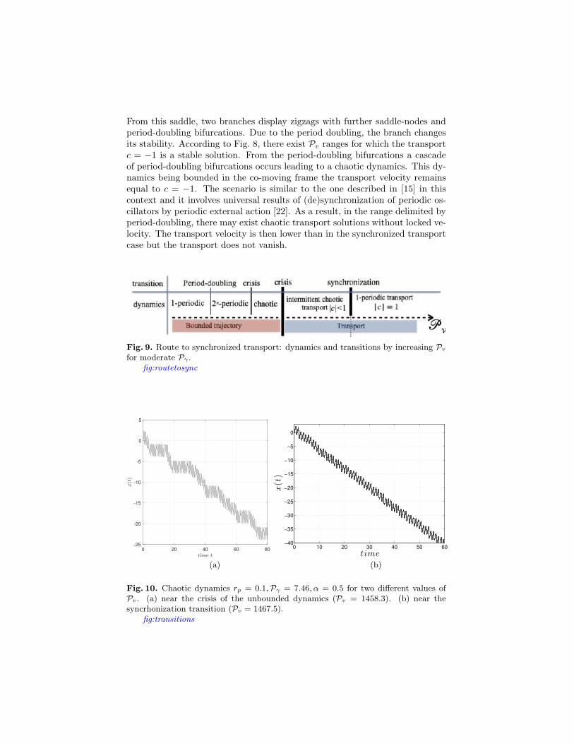
From this saddle, two branches display zigzags with further saddle-nodes andperiod-doubling bifurcations. Due to the period doubling, the branch changesits stability. According to Fig. 8, there exist Pv ranges for which the transportc = −1 is a stable solution. From the period-doubling bifurcations a cascadeof period-doubling bifurcations occurs leading to a chaotic dynamics. This dy-namics being bounded in the co-moving frame the transport velocity remainsequal to c = −1. The scenario is similar to the one described in [15] in thiscontext and it involves universal results of (de)synchronization of periodic os-cillators by periodic external action [22]. As a result, in the range delimited byperiod-doubling, there may exist chaotic transport solutions without locked ve-locity. The transport velocity is then lower than in the synchronized transportcase but the transport does not vanish.
Fig. 9. Route to synchronized transport: dynamics and transitions by increasing Pvfor moderate Pγ .
fig:routetosync
0 20 40 60 80
-25
-20
-15
-10
-5
0
5
0 10 20 30 40 50 60−40
−35
−30
−25
−20
−15
−10
−5
0
time
x(t)
(a) (b)
Fig. 10. Chaotic dynamics rp = 0.1,Pγ = 7.46, α = 0.5 for two different values ofPv. (a) near the crisis of the unbounded dynamics (Pv = 1458.3). (b) near thesyncrhonization transition (Pv = 1467.5).
fig:transitions
139

4.2 chaotic transitions
The synchronization transition at the saddle-node of Fig. 8 (Pv = 1628,Pγ =7.46) differs from the synchronization at Pγ = 24.1. The dynamics is no longerquasi-periodic but chaotic. In [15], we found intermittency occuring at chaotictime intervals: this behavior is typical of large forcing of an oscillator [22].However, the particle dynamics displayed in Fig. 10b does not corroborate theexistence of intermittency. We guess that the coexistence of attractors hidesthe intermittency.Now, we detail the transitions from the periodic solutions to the synchronizedtransport by increasing Pv when Pγ = 7.46. Indeed, we retrieve all the bifurca-tions scenario explained in detail in [15]. The route to synchronized transportis sketched in Fig. 9. The periodic solutions s0 or sm (Fig. 2), by increasing Pv,involve a period-doubling cascade leading to a chaotic unbounded dynamics. Amerging crisis may appears and because of the spatial periodicity the strangeattractor is no longer bounded. If the problem does not have the parity sym-metry (α 6= 0), we expect a preferential direction. In Fig. 10a, the dynamics ofthe particle near the onset displays a drift to negative values in a intermittentmanner. However, the intermittency is not quasi-periodic but chaotic. By in-creasing further Pv, the drift velocity increases and the dynamics is still chaotic(Fig. 10b).
4.3 Chaotic drift
0 200 400 600 800 1000−500
−400
−300
−200
−100
0
100
time t
xn
Fig. 11. Stroboscopic particles positions xn at entire times for radii rp = 0.05 (blacklines) and rp = 0.1 (red lines) for eleven initial conditions (x0, v0) = (0, i/10) withi = 0, 1, . . . , 10. Other parameters are α = 0.1,Pγ = 6.7,Pv = 2000.
fig:tchaos
140

The previous transport solutions are obtained for α = 0.5 and we find onlytransport to negative direction. A non-zero value of α is required for the ex-istence of intermittent and quasi-periodic drift. However, if Pγ is not large,unbounded dynamics and also synchronized transport may exist for α = 0.The scenario from periodic solution to the unbounded dynamics in Fig. 9 in-volves, this time, spontaneous symmetry breaking. The chaotic dynamics hasdiffusion like behavior: no prefential direction is observed. When there is asynchronized transport then the synchronized transport solution in the oppo-site direction exists too. To have an effective transport, we need to slightlybreaks the parity symmetry. As explained in [23], the transport solutions stillexist but for slightly different parameter ranges when α is small. Therefore, weexpect there is parameter domains for which the transport direction dependson the particle size.We found for α = 0.1,Pγ = 6.7 and Pv = 2000 different drift directions de-pending on the particle size: a net drift appears for rp = 0.1 and while, forrp = 0.05, a slight drift to positive direction occurs (Fig. 11). The dynamicsis chaotic and notably it depends on the initial conditions. For rp = 0.05, themean value over the initial conditions of the velocity transport is slightly posi-tive (c ' 0.04). In addition, there is a diffusive-like behavior too: the trajectorydeviation increases with the time. Indeed, the chaotic dynamics results fromthe competition between opposite transport solutions c = ±1 which are unsta-ble. For rp = 0.1 the diffuse behavior is weak and the mean velocity remainsclose to c = −2/5. A possible explanation is that we are in the vicinity of theonset of the synchronized transport c = −2/5. The multiplicity of solutionsmakes it difficult to find this synchronized transport.
5 Concluding remarks
We have shown using time-integration and bifurcation analysis that a selectivetransport of micro-particles is possible depending on the particle size.For large drag Pγ , the possible slow drift is quasi-periodic and determined bythe pumping asymmetry, i.e. the parameter α. Then, the drift requires a nonzero value of α typically a value about 0.5. By decreasing the drag Pγ wefound out synchronized transport solutions. The velocity is then locked to arational value. If α is about 0.5, the transport velocity is negative. Therefore,for α about 0.5, we found either bounded periodic solutions or transport inthe negative direction. However, if the selectivity is possible, we do not find achange of transport direction depending on the particle size.Such a property was found for moderate value of Pγ < 10 and α about 0.1.Indeed, for this parameters values, the asymmetry of the problem is no longerrequired. We retrieved the scenarios of the ratchet problem of a point-likeparticle. In particular, the dynamics can be chaotic. We found parameterssuch as the direction of the parameter drift depends on the particle size.This theoretical study may have application of heavy particles in the air inmicro-gravity environment. Indeed, the small value of Pγ requires a low densityfluid and the gravity could break the phenomena transport. Because of the
141

chaotic dynamics could be strongly influenced by the noise [24], a further workwould be to study the influence of noise on the transport selectivity.
References
1. Kulrattanarak T., van der Sman R., Schroenn C. and Boom R. Advances in Colloidand Interface Science142200853 .
2. Pamme N. Lab Chip2007716441659.
3. Huang R., Barber T. A., Schmidt M. A., Tompkinsand R. G., Toner M., BianchiandD. W., Kapur R. and Flejter W. L. PRENATAL DIAGNOSIS282008892.
4. Hasni A. E., Gobbels K., Thiebes A., Braunig P., Mokwa W. and SchnakenbergU. Procedia Engineering2520111197 eurosensorsXXV.
5. Autebert J., Coudert B., Bidard F.-C., Pierga J.-Y., Descroix S., Malaquin L.and Viovy J.-L. Methods572012297 flow Cytometry and Cell Sorting: the NextGeneration.
6. Lee G.-H., Kim S.-H., Ahn K., Lee S.-H. and Park J. Y. Journal of Micromechanicsand Microengineering262016013003.
7. Loutherback K., Puchalla J., Austin R. H. and Sturm J. C. Phys. Rev.Lett.1022009045301.
8. Matthias S. and Muller F. Nature424200353.
9. Santamaria F., Boffetta G., Afonso M. M., Mazzino A., Onorato M. and PuglieseD. EPL (Europhysics Letters)102201314003.
10. Reimann P. Physics Reports361200257.
11. Hanggi P. and Marchesoni F. Rev. Mod. Phys.812009387.
12. Kettner C., Reimann P., Hanggi P. and Muller F. Phys. Rev. E612000312.
13. Makhoul M., Beltrame P. and Joelson M. International Journal of Mechan-ics92015260.
14. Luchsinger R. H. Phys. Rev. E622000272.
15. Beltrame P., Makhoul M. and Joelson M. Phys. Rev. E932016012208.
16. Makhoul M., Beltrame P. and Joelson M. Particle drag force in a periodic channel:wall effects in proc. of Topical Problems of Fluid Mechanics : Proceedings, Prague2015 pp. 141–148.
17. Brenner H. Journal of Fluid Mechanics181964pp 144.
18. Makhoul M. Modelisation du transport de particule dans un ecoulement de stokesa effet cliquet Ph.D. thesis Universite d’Avignon (juillet 2016).
19. Pomeau Y. and Manneville P. Commun. Math. Phys.741980189.
20. Wickenbrock A., Cubero D., Wahab N. A. A., Phoonthong P. and Renzoni F.Phys. Rev. E842011021127.
21. Cuesta J. A., Quintero N. R. and Alvarez-Nodarse R. Phys. Rev. X32013041014.
22. Pikovsky A., Rosenblum M. and Kurths J. International Journal of Bifurcationand Chaos1020002291.
23. Beltrame P. The Foundations of Chaos Revisited: From Poincare to Recent Ad-vancements Understanding Complex Systems (Springer) 2016 Ch. Absolute Neg-ative Mobility in a Ratchet Flow pp. 249–261.
24. Beltrame P. Journal of Chaotic Modeling and Simulation12018101.
25. Bhagat A. S., Kuntaegowdanahalli S. S. and Papautsky I. Microfluidics andNanofluidics72009217.
26. Dijkshoorn J., Schutyser M., Wagterveld R., Schron C. and Boom R. Separationand Purification Technology173201786 .
142

27. G. D’Amico, J. Janssen and R. Manca. Homogeneous semi-Markov reliabilitymodels for credit risk management. Decisions in Economics and Finance, 28, 2,79–93, 2005.
28. J. Janssen and R. Manca. Semi-Markov risk models for finance, insurance andreliability, Springer, New York, 2007.
29. J. Janssen and C.H. Skiadas. Dynamic modelling of Life-Table data, AppliedStochastic Models and Data Analysis, 11, 1, 35–49, 1995.
30. G. Saporta. Probabilites, Analyse des Donnees et Statistique, Editions Technip,Paris, 1990.
31. C. H. Skiadas and C. Skiadas. Chaotic Modeling and Simulation: Analysis ofChaotic Models, Attractors and Forms, Taylor and Francis/CRC, London, 2009.
143

144

Chaotic Modeling and Simulation (CMSIM) : –, 2020
Application of New 4-D Chaotic Map forSecure IP-Communications
Belqassim Bouteghrine1, Camel Tanougast2, and Said Sadoudi3
1 LCOMS, Universite de Lorraine, 57070 Metz, France(E-mail: [email protected])
2 LCOMS, Universite de Lorraine, 57070 Metz, France(E-mail: [email protected])
3 Ecole Militaire Polytechnique, 16000 Algiers, Algeria(E-mail: [email protected])
Abstract. Chaos systems have been studied for decades due to their applications inseveral domains such as: economy, communications, cryptography. . . etc. In recentyears, designing and proposing new and higher dimensional chaotic systems becomean increased tendency in particular for chaotic systems applied in network securitydomain.In this paper, we propose a new 4-dimension chaotic map with four (04) control pa-rameters and five (05) non-linear terms. Then, we investigate the chaotic behaviorsof the proposed system by considering the bifurcation and the Lyapunov exponents(LE) theories. The proposed map is applied for generating cipher keys to performdata encryption and secure an Internet Protocol (IP) communication.Keywords: Chaotic, Dimension, Bifurcation, Lyapunov exponents, Network secu-rity, Encryption, IP-communication.
1 Introduction
Chaos systems have been studied for decades due to their applications in severaldomains such as: electronic circuits [1],[2], network security [3],[4], encryptiondomain [5],[6] and in power control [7]. In one hand, chaotic systems’ proper-ties have been studied and investigated using the bifurcation and the Lyapunovexponents theories [8],[9]. In the other hand, among the existing chaotic sys-tems, researchers have investigated for new and more complex systems. Bycombining two coexisting attractors, in [10] the evolution of a new 4-dimensionchaotic system is presented and analyzed by using bifurcation diagrams andLyapunov exponents’ spectrum. In [11] authors proved that using only sineor cosine functions and modifying two (02) variables in the function, n-scrollattractors can be generated. Moreover looking for higher dimension, a new 4-Dhyperchaotic continuous time system is introduced in [15] and its main spec-ifications are analyzed by means of equilibrium points, stabilities and power
Received: / Accepted:© 2012 CMSIM ISSN 2241-0503
145

2 B. Bouteghrine et al.
spectrum. In [16] authors showed that, using 4-D Lorenz system for secureTCP communicationonl, consume a huge amount of ressources and computa-tions.Consequently, we present through this paper an optimized new 4-dimensionaldiscrete time system for encryption purpose. Then, the chaotic behavior ofthe proposed map is investegated based on the bifurcation and Lyapunov ex-ponent theories. The rest of this paper is structured as follows. The 4-D mapis introduced and the chaotic behavior is investigated in section II. In SectionIII, software implementation of secure communication is illustrated using theproposed map. Finally, a conclusion is given in section IV.
2 The Proposed 4-D Map
2.1 System Description
The proposed 4-D map with (04) bifurcation parameters and (05) non-linearterms is given as follows:
X(n + 1) = 1− a ∗X(n)2 + (Y (n) ∗ Z(n) ∗ P (n))
Y (n + 1) = 1− b ∗ Y (n)2 + (X(n) ∗ Z(n) ∗ P (n))
Z(n + 1) = c ∗ (X(n) ∗ Y (n) ∗ P (n))
P (n + 1) = d ∗X(n)
(1)
Where X, Y , Z and P are the state variables and a, b, c, d are the controlparameters or the bifurcation parameters.
2.2 Chaos Behavior Investigation
Following the lines given in [12] and [13], the chaotic behavior of the proposedsystem (1) is investigated by considering mainly the bifurcation and the Lya-punov exponents (LE) theories.
Bifurcation processBifurcation theory is concerned with changes in the solutions’ behavior of the
proposed system (1) as the parameters a, b,c and d are varying.Figure 1 shows that chaotic behavior appears in several intervals of the param-eters a ∈[0.22, 1.00], b ∈[0.90, 2.00], c ∈[-0.95, 0.95] and for the values of theparameter d ∈[-1.05, 2.5].
146

Chaotic Modeling and Simulation (CMSIM) : –, 2012 3
Fig. 1. The bifurcation graphs of the proposed 4-D map.
LE processComputing the LE values gives a possibility not only to detect all resonances
in the response function, but also to detect the presence of chaos [14]. To searchfor strange attractors or for chaos in the proposed model (1), we proceed asfollows:First, we select the values of the parameters a, b,c and d calculated in the pre-vious step (bifurcation process). Then we iterate equations (1) repeatedly untilthe Lyapunov exponent becomes small or negative, in which case the solutionis probably a fixed point or limit cycle. In either event, we choose a differentcombination of a, b,c, d and start over the process.If, after a few thousand iterations, the solution is bounded (not enormous)and the Lyapunov exponent is positive, then it is likely that you have found astrange attractor that corresponds to the chosen values of a, b,c and d.
As a final result, the chaotic behavior is obtained and illustrated by thetrajectory graphs and the signal graphs in figures 3 and 4, respectively.
147
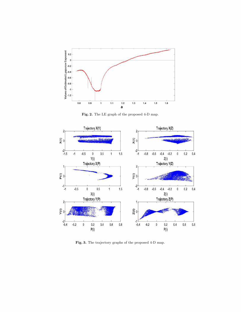
Fig. 2. The LE graph of the proposed 4-D map.
Fig. 3. The trajectory graphs of the proposed 4-D map.
148
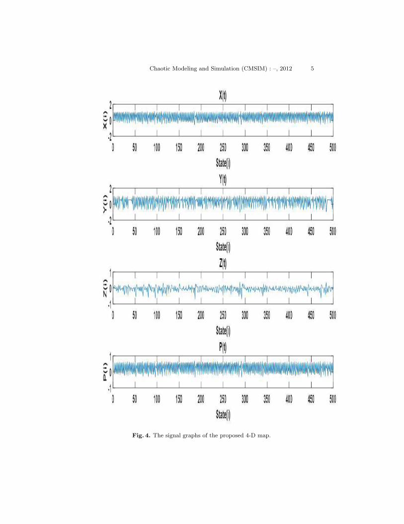
Chaotic Modeling and Simulation (CMSIM) : –, 2012 5
Fig. 4. The signal graphs of the proposed 4-D map.
149

6 B. Bouteghrine et al.
3 software implementation of secure Communication
Chaotic systems have been introduced in the network communication securitydomain since that they are characterized by their sensitivity, unpredictabilityand their widespread spectrum. Hence; we propose to introduce the 4-D chaosmap for securing Client-Server Communication. In the first order, we pre-pare the Client-Server platform composed of two (02) client stations connectedthrough an Ethernet network to one (01) server machine (Figure 5).
Fig. 5. The platform test bench.
The proposed platform works considering the following steps :- The server listens for client connections;- The client initiates the connection;- The connection is established;- The key-Generator load the first random sequence and the next sample;- The client uses the first key to encrypt and send data to the server;- The server use the same key to decrypt and send confirmation of receivingdata;Finally, the client terminates the communication by closing the channel, andthe key-Generator module saves samples for next use with the server.
In the second order, we develop a C# software application for exchang-ing securely messages between connected computers (figure 7).The developedapplication includes a chaos-based cryptosystem using the proposed 4-D mapwhich is described by the system (2); with a=1.55; b= 1.7; c= 1.6; d= 0.40.Considering that we are targeting to generate a 32-bit key using the chosenmap, then we have the key space of the cryptosystem 232∗(4+4)=2256 whichis considered very good value in for encryption since that the required value
150

Chaotic Modeling and Simulation (CMSIM) : –, 2012 7
should be more than 2100 to satisfy the encryption requirements for key space[16].
Fig. 6. The developped application’s interface.
4 Conclusion
In recent years; researching and developping new and higher dimensional chaoticsystems become a rising trend in perticular for secure communication purposes.In this paper, we propose new 4-Dimensional chaotic map in first order. Sec-ondly, the chaotic behavior of the proposed system is investigated using analgorithm based on the bifurcation and the Lyapunov exponents properties.Finally, we apply the proposed system to generate random keys in order toperform a secure IP-communication.As future work, statistical and security tests of the proposed system will beconsidered as well as the hardware implementation of the proposed scheme.
151

8 B. Bouteghrine et al.
References
1.Y. Zhou, Z. Hua, C. M. Pun and C. L. Philip Chen. Cascade Chaotic System WithApplications. IEEE Trans. Cybern., vol. 45, no 9, pp. 2001-2012, Sept. 2015.
2.G. Mykolaitis. Temperature-stable hyperchaotic oscillator.IEEE Trans. CircuitsSyst. Fundam. Theory Appl., vol. 45, no 11, pp. 1198-1200, Nov. 1998.
3.A. Chonka, J. Singh and W. Zhou. Chaos theory based detection against networkmimicking DDoS attacks.IEEE Commun. Lett., vol. 13, no 9, pp. 717-719, Sept.2009.
4.Y. Chen, X. Ma and X. Wu. CDDoS detection algorithm based on preprocessingnetwork traffic predicted method and chaos theory.IEEE Commun. Lett., vol. 17,no 5, pp. 1052-1054, May. 2013.
5.X. Zhang, L. Wang, Z. Zhou, and Y. Niu. A Chaos-Based Image Encryption Tech-nique Utilizing Hilbert Curves and H-Fractals.IEEE Access, vol. 7, pp. 74734-74746, 2019.
6.U. Cavusoglu, A. Akgul, S. Kacar, I. Pehlivan, and A. Zengin. A novel chaos-basedencryption algorithm over TCP data packet for secure communication.Secur.Commun. Netw., vol. 9, no 11, pp. 1285-1296, 2016.
7.A. Al Talabani, A. Nallanathan and H. X. Nguyen. A Novel Chaos Based CostFunction for Power Control of Cognitive Radio Networks. IEEE Commun. Lett.,vol. 19, no 4, pp. 657-660, Apr. 2015.
8.J. C.Sprott. Chaos and Time-Series Analysis. Oxford: Oxford University Press, vol.69.2003.
9.Z. Sandor, B. Erdi, A. Szell, and B. Funk. The Relative Lyapunov Indicator: AnEfficient Method of Chaos Detection.Celest. Mech. Dyn. Astron., vol. 90, no 1,pp. 127-138, Jul. 2004.
10.Q. Lai, C. Chen, X. W. Zhao, J. Kengne, and C. Volos. Constructing ChaoticSystem With Multiple Coexisting Attractors.IEEE Access, vol. 7, pp. 24051-24056, 2019.
11.W. K. S. Tang, G. Q. Zhong, G. Chen, and K. F. Man. Generation of n-scrollattractors via sine function.IEEE Trans. Circuits Syst. Fundam. Theory Appl.,vol. 48, no 11, pp. 1369-1372, Nov. 2001.
12.C. Shen, S. Yu, J. Lu, and G. Chen. A Systematic Methodology for ConstructingHyperchaotic Systems With Multiple Positive Lyapunov Exponents and CircuitImplementation.IEEE Trans. Circuits Syst. Regul. Pap., vol. 61, no 3, pp. 854-864, mar 2014.
13.C. J. Feng, X. Z. Li, and L. Y. Liu. Bifurcation and global dynamical behavior ofthe f(T) theory.Mod. Phys. Lett. A, vol. 29, no 07, pp. 1450033, Mar. 2014.
14.J. K. Hunter. Introduction to dynamical systems. U.C.Davis Mathematics MAT A,207. 2011.
15.M. A.ABABNEH. New four-dimensional chaotic attractor. Ain Shams EngineeringJournal, vol. 9, no 4, pp. 1849-1854, 2018.
16.B. Bouteghrine, M. Rabiai, C. Tanougast and S. Sadoudi. Hardware Implemen-tation of Secured Socket Communication based on Chaotic Cryptosystem. 2019International Conference on Cyber Security and Protection of Digital Services(Cyber Security), Oxford, United Kingdom, 2019, pp. 1-4, doi: 10.1109/Cyber-SecPODS.2019.8884879.
152

Liutex-based analysis of vortex in two-phase flow past2D cylinder using LBM on GPU
Pengxin Cheng1, Nan Gui1, Xingtuan Yang1, Jiyuan Tu1,2, Shengyao Jiang1, andHaijun Jia1
1 Institute of Nuclear and New Energy Technology, Collaborative Innovation Center ofAdvanced Nuclear Energy Technology, Key Laboratory of Advanced Reactor Engineeringand Safety of Ministry of Education, Tsinghua University, Beijing, 100084, People’sRepublic of China.(E-mail: [email protected])
2 School of Engineering, RMIT University, Melbourne, VIC 3083, Australia
Abstract. Two-phase flow past obstacle is widely applied in industries and engineering, wherethe interaction of different phases coupled with influence of solid is rather complex. In thiscontext, the flow characteristics and vortex field have been investigated to explore the mechanismof two-phase drag and vortex variation. The Lattice Boltzmann Method is utilized to studythe multi-component multiphase flow. The computation implemented on GPU is remarkablyaccelerated owing to the natural parallelism of LBM. The process of two-phase flow past a 2Dcylinder is thoroughly examined. The drag forces including the total force and the componentscaused by dispersed phase and continuous phase respectively, are illustrated, and themechanismsfor the variations have also been explained. Meanwhile, the vortex-identification approachesbased on the Liutex as well as traditional methods are compared. The relationship betweenthe breakup as well as coalescence process and extremums of different vortex identificationvariables is analyzed.Keywords: Two-phase flow, flow past cylinder, LBM, vortex identification, Liutex.
1 Introduction
Flow past obstacles is a ubiquitous phenomenon encountered in various industriesincluding chemical process, food processing and power engineering. For decades,numerous experimental and numerical efforts have been made focusing on drag andlift force, vortex separation, flow-induced vibration, etc. The two-phase flow pastobstacles plays a significant role in practical application, such as the packed bedreactor in petroleum chemical process and heat exchangers in power industry.
In view of the impact of bubbles on the solid, the influence of bubble movementon vortex shedding and the involvement of bubbles into the vortex, the interaction intwo-phase cross flow between three phases, namely solid, liquid and gas, is coupledand intricate. Under this circumstance, the traditional computational fluid dynamics(CFD) methods like Finite Volume Method (FVM) might encounter difficulties andfail to acquire the details of flow field from macroscopic scale.
Endowed with the advantage of flexible geometry characteristics, inherent paral-lelism and simplicity of implementation, the Lattice Boltzmann method (LBM) has
153

witnessed rapid development in the past decades, particularly in the field of multiphaseflow and flow in complex geometry. Based on the molecular kinetic theory, the LBMprovides a novel and potent approach with solid background of physics and efficientalgorithm in multi-scale analysis from the mesoscopic perspective. With the com-putation largely restricted to local nodes, the LBM is ideal for implementation withparallelized hardware such as GPU, which shows an apparent advantage over CPU inHigh Performance Computing. The implementation of LBM on GPU contributes toboosting computation speed and achieving reliable acceleration performance.
As a fundamental research target, the vortex is of vital significance for an intuitiveunderstanding of turbulence. After decades of intensive research, there are still plentyof ambiguous issues left to be solved including a widely-acknowledged definition ofvortex. The vortex identification method has evolved from the first generation intuitivevorticity-based method that fails to discriminate rotational motion from a shear layerin viscous turbulent flow, to the second generation that rely on other eigenvalue-basedparameters including∆, λ2, λci , etc., which are unfortunately dependent on case-relateduncertain threshold and unable to capture the vortical strength to some extent.
Recently Gao and Liu put forward the third generation Liutex method [1,2], whichprovides a more precise perspective of defining vortex. According to the theory,the vorticity could be decomposed into the non-rotational part, mainly shear and therotational part called Liutex, namely ®ω = ®S + ®R. The direction of Liutex vector,representing the local rotation axis, is defined via the real eigenvector of the velocitygradient tensor. Themagnitude of Liutex, used to quantify the local rotational strength,could be simply determined by a explicit formula proposed byWang [3], which followsthe idea of getting rid of the non-rotational part from the vorticity. With the aid ofLiutex, continuous research has been conducted on various applications including thehairpin vortices [4] and vortex in swirling jets [5,6].
This paper will present a comprehensive investigation on the flow and vortexfield and drag force of multiphase flow past cylinder. The variation of multiphasedrag force with the movement of fluid will be analyzed. The detailed evolutionof the primary variables during the bubble deformation will be discussed for a deepunderstanding of its relationshipwith vortex generation and development. Awide rangeof identification parameters including the Liutex will be evaluated. The relationshipbetween extremums of different vortex identification variables and bubble deformationprocess, mainly the breakup as well as coalescence, will be analyzed.
2 Models and methods
2.1 Basics of Lattice Boltzmann Method
Lattice Boltzmann Method could be derived from the Boltzmann equation based onthe kinetic molecular dynamics.
∂ f∂t+ ®ξ · ∇®x f + ®a · ∇ ®ξ f = Ω( f ), (1)
154

where f (®x, ®ξ, t) denotes the particle distribution function that represents the densityof particles with velocity ®ξ at position ®x and time t. The collision operator Ω f
characterizes microscopic interaction between molecules and could be simplified bysingle-relaxation-time approximation proposed by Bhatnagar–Gross–Krook (BGK)[7].
Ω( f ) = −f − feqτ
(2)
Through discretizing in the physical space, velocity space and time, the discreteLattice Boltzmann Equation (LBE) could be derived,
fi(®x + ®ciδt, t + δt) − fi(®x, t) = (Ω(®x, t) + Fi(®x, t))δt (3)
where ®ci represents the discrete velocity direction, and fi(®x, t) is the particle distributionfunction along the direction of ®ci . The widely adopted discretization model is usuallyexpressed as DdQm, where d and m denotes number of dimensions and velocities. For2D simulation D2Q9 is adopted.
The macroscopic parameters such as density, velocity and internal energy can becalculated statistically from moments of the discrete distribution function.
ρ =∑i
fi, ρ®u =∑i
ci fi, ρe =12
∑i
( ®ci − ®u)2 fi . (4)
By means of the multi-scale expansion techniques such as Chapman-Enskog anal-ysis, the LBGK model could recover continuity equation and Navier-Stokes equationat the macroscopic scale under the limit of small Mach number.
2.2 Multiphase Lattice Boltzmann methods
In multiphase flow simulation, the Shan-Chen model [8] incorporates a repulsiveor attractive Shan-Chen force, which does not need any explicit interface tracking.Compared with other models, the Shan-Chen model has satisfactory performance inboth efficiency and accuracy and is adopted in the multiphase LBM simulation.
For single-component multiphase flow, the interaction force density acting on fluidat ®x can be computed via integral over all possible interaction sites ®x′ .
FSC(®x) = −∫(®x′
− ®x)G(®x, ®x′
)ψ(®x)ψ(®x′
)d3 ®x′
(5)
where ψ(ρ) also called pseudo-potential denotes the effective density. G(®x, ®x′
) is aGreen function to determine the strength and range of interaction, with the simplestform concerning nearest lattice neighbors.
G(®x, ®x′
) =
wiG ®x
′
= ®x + ®ciδt
0 otherwise(6)
155
In a multiphase fluid system constituted by n components, the LBE of Shan-Chenmodel can be expressed as
f σi (®x + ®ciδt, t + δt) − f σi (®x, t) =f eq(σ)i − f σi
τσδt + (1 −
δt2τσ)Fσ
i (®x, t) (7)
where f σi , f eq(σ)i , τσ,Fσi is the distribution function, equilibriumdistribution function,
relaxation time and forcing term of the σ component.The total interaction force acting on the σ component can be computed by adding
the force imposed by all the components.
FσSC(®x) = −ψ
σ(®x)∑σ′
Gσσ′
∑i
wiψσ′
(®x + ®ciδt) ®ciδt (8)
In the present work we focus on the two-component multiphase system withoutphase change, namely n = 2 and Gσσ = 0. Gσσ
′ is set as positive for repulsiveforce between different components. The overall density, weighed average velocityand pressure of the fluid are calculated as follows.
ρ =∑σ
ρσ, ®u =∑σ(ρσ ®uσ/τσ)∑σ(ρσ/τσ)
, p = c2s (ρσ + ρσ′ ) + c2
sGρσρσ′ (9)
2.3 Momentum Exchange Algorithm of the Bounce-Back methodThe widely adopted method to implement no-slip wall boundary condition in LBMis the Bounce-Back method, with the advantage of simplicity of implementation andguaranteed mass conservation. However, the traditional Bounce-Back method in theregular lattice could only approximate arbitrary boundaries with stair-case shapes,which might introduce large errors at cells nearby boundaries. While by increasing themesh resolution the error could be reduced and the results approaches precise solution.
In the context of Bounce-Back scheme, the Momentum Exchange Algorithm(MEA) is adopted to calculate the force in this paper. The basic idea of MEA isto identify the populations across the boundary and calculate the net momentum trans-fer consisting of two parts, namely the momentum carried by the fluid to the wall f iniand the momentum transported from the wall to the fluid f out
i. The procedure includes
the following steps [9].• Identify the momentum links between solid and boundary nodes xwi .• Evaluate the incoming populations f ini and bouncing populations f out
iof each
momentum link.• Calculate the transferred momentum during the time steps and acting force on theboundary.The drag and lift forces are calculated using MEA in the following section. The
drag force FD is to quantify the resistance in the opposite direction of flow. The liftforce FL is in the orientation perpendicular to the flow direction. Thus they can beevaluated by the components of total force in X and Y direction. Since the force is cal-culated via the populations f , for the multi-component case in present paper, the forceof theσ component could be obtained based on the populations of each component f σ .
156

2.4 Parallel Implementation of LBM on GPU
For practical convenience, the main process of calculation of LBE can be decomposedinto two parts, namely collision and streaming. With the features of ‘non-linearity islocal’ in collision step and ‘non-locality is linear’ in streaming step, LBM is naturallysuitable for computation on parallel architecture including GPU. GPU is capable of ex-ecuting a multitude of threads in parallel simultaneously. which could take advantageof thousands of cores in GPU and remarkably boost the computation. The implemen-tation of LBM on GPU has aroused wide research interest and proved successful indelivering reliable performance. In this paper, the open-source software Sailfish isadopted for the simulation. The computation was implemented on NVIDIA Tesla K20GPU.
2.5 Vortex identification method and Liutex
Several well-acknowledged identification parameters are selected including the vor-ticity ω [10], Q [11], R [12], Ω [13], ΩR [14] and Liutex R [15], which are definedby:
ω = ‖ ®ω‖ = ‖∇ × ®u‖
Q =12(‖B‖2F − ‖A‖
2F )
Ω =‖B‖2F
‖A‖2F + ‖B‖2F
=b
a + b
ΩR =β2
α2 + β2 + ε
®R = R®r =(〈 ®ω, ®r〉 −
√〈 ®ω, ®r〉2 − 4λ2
ci
)®r
(10)
where A = 12 [∇®u + (∇®u)
T ], B = 12 [∇®u − (∇®u)
T ] are the symmetric and antisym-metric parts of the velocity gradient tensor, respectively. a = ‖A‖2F , b = ‖B‖2F ,
where ‖ · ‖2F represents the Frobenius norm. α = 12
√(∂V∂Y −
∂U∂X
)2+
(∂V∂X +
∂U∂Y
)2
and β = 12
(∂V∂X −
∂U∂Y
), where while U, V and W represent the velocity compo-
nents in the XYZ coordinate satisfying ∇®V = Q∇®uQT by a rotation matrix Q and[∇ ®V]1,3 = [∇ ®V]2,3 = 0. ε is a small positive parameter. λci and ®r are the imaginarypart of the complex eigenvalue and the real eigenvector of ∇®u, respectively. In thiswork, these criteria will be used for comparative analysis of vortex motion.
2.6 Validation
In this section, the LBM model is firstly validated against 2D single-phase flow past acylinder to verify the accuracy of force evaluation. Then the Laplace test is conductedto examine the multiphase model.
157

For two-dimensional case, with the characteristic length corresponding to theobstacle’s diameter, the drag and lift coefficient and the Strouhal number are calculatedas follows.
CD =FD
12ρDu2
, CL =FL
12ρDu2
, St =f Du
(11)
The comparison of simulation results with validation reference is displayed in Table1. On the whole, the simulation results show in good conformity with benchmark inSchaefer’s paper[16].
As for the multi-component Laplace test, a spherical droplet of one phase withradius R is initialized surrounded by the another liquid phase. The interface is deter-mined where the density reaches the average of the bulk densities inside and outsidethe droplet. The result of Laplace test is displayed in Fig. 1, where the relationshipbetween measured pressure difference ∆p and 1/R is linear, with coefficient of deter-mination of the fitted lines above 0.999, in desirable agreement with the Laplace Law,namely ∆p = σ/R.
Concerning the two-phase model validation, it has been completed in our earlierwork [17], by the validating the bubble departure diameter and release period. Inaddition, the GPU performance of LBM has also been tested and validated via thecavity driven flow case in another earlier work [18].
On the whole, the LBMmode, two-phase scheme, GPU performance have alreadybeen well validated.
(a) Density contour (b) Data fitting
Fig.1. The validation of Laplace test for multi-component case
3 Results and discussion
3.1 Numerical setup
Theflowdomain is discretized by 256×1024Cartesianmesh grids. The two-dimensionalcylinder obstacle with the diameter of 100 nodes is placed right in the center of channeland referred to as cylinder in the following sections. Initially a circular bubble of the
158
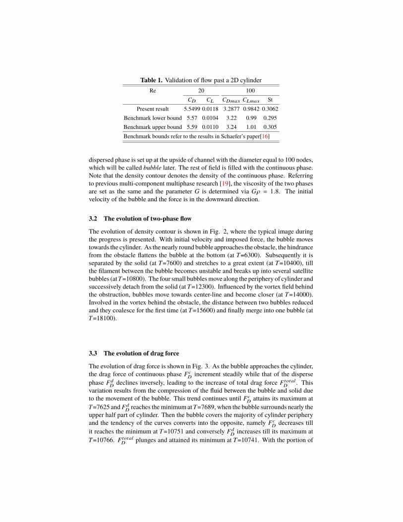
Table 1. Validation of flow past a 2D cylinderRe 20 100
CD CL CDmax CLmax StPresent result 5.5499 0.0118 3.2877 0.9842 0.3062
Benchmark lower bound 5.57 0.0104 3.22 0.99 0.295Benchmark upper bound 5.59 0.0110 3.24 1.01 0.305Benchmark bounds refer to the results in Schaefer’s paper[16]
dispersed phase is set up at the upside of channel with the diameter equal to 100 nodes,which will be called bubble later. The rest of field is filled with the continuous phase.Note that the density contour denotes the density of the continuous phase. Referringto previous multi-component multiphase research [19], the viscosity of the two phasesare set as the same and the parameter G is determined via Gρ = 1.8. The initialvelocity of the bubble and the force is in the downward direction.
3.2 The evolution of two-phase flow
The evolution of density contour is shown in Fig. 2, where the typical image duringthe progress is presented. With initial velocity and imposed force, the bubble movestowards the cylinder. As the nearly round bubble approaches the obstacle, the hindrancefrom the obstacle flattens the bubble at the bottom (at T=6300). Subsequently it isseparated by the solid (at T=7600) and stretches to a great extent (at T=10400), tillthe filament between the bubble becomes unstable and breaks up into several satellitebubbles (atT=10800). The four small bubblesmove along the periphery of cylinder andsuccessively detach from the solid (at T=12300). Influenced by the vortex field behindthe obstruction, bubbles move towards center-line and become closer (at T=14000).Involved in the vortex behind the obstacle, the distance between two bubbles reducedand they coalesce for the first time (at T=15600) and finally merge into one bubble (atT=18100).
3.3 The evolution of drag force
The evolution of drag force is shown in Fig. 3. As the bubble approaches the cylinder,the drag force of continuous phase Fc
D increment steadily while that of the dispersephase Fd
D declines inversely, leading to the increase of total drag force FtotalD . This
variation results from the compression of the fluid between the bubble and solid dueto the movement of the bubble. This trend continues until Fc
D attains its maximum atT=7625 and Fd
D reaches theminimum atT=7689, when the bubble surrounds nearly theupper half part of cylinder. Then the bubble covers the majority of cylinder peripheryand the tendency of the curves converts into the opposite, namely Fc
D decreases tillit reaches the minimum at T=10751 and conversely Fd
D increases till its maximum atT=10766. Ftotal
D plunges and attained its minimum at T=10741. With the portion of
159

(a) T=6300 (b) T=7600 (c) T=10400 (d) T=10800
(e) T=12300 (f) T=14000 (g) T=15600 (h) T=18100
Fig.2. The contour of density at different time steps
bubble coverage of cylinder periphery increasing, FdD consequently enhances and Fc
Dreduces, until the bubble is over stretched and break up into pieces. Therewith thecontinuous phase regains the contact with cylinder and Fc
D boosts, arriving at a localmaximum at T=11633. In contrast Fd
D drops towards a local minimum at T=11617.Afterwards the curves gradually flatten out.
Fig.3. The evolution of drag force
160

3.4 The evolution of R, S, ω and comparison of vortex identification methods
Based on the relation of ®R + ®S = ®ω, the evolution of R,S and vorticity ω at differenttime steps are shown in Fig. 4 and Fig. 5.
For the evolution of breakup process in Fig. 4, before bubble brings into contactwith solid, some zones with negative Liutex appear inside the bubble in the bottomand lateral at T=6300. As the deformation affects the distribution of Liutex, there existnegative zone in the center and positive zone on the sides atT=7600. AtT=10400 thereexist zones with positive Liutex between and ahead of the stretched bubbles, as wellas zones with negative Liutex laterally adjacent to them. When the break-up of bubbleoccurs at T=10800, magnitude of Liutex near the position of fracture is relatively highin positive or negative value. As the surface tension transform the bubble into a nearlyround shape at T=11600 and T=12300, zones with high magnitude of negative Liutexinside the bubbles are observed.
For the evolution of coalescence process in Fig. 5, when the small bubbles mergetogether, the distortion results in zones with high level of magnitude of Liutex bothinside and around the bubble. Taking the coalescence of two bubbles in the right as anexample, atT=15500 there appear negative Liutex zone near the line of bubble contact.At T=15600, there are positive Liutex zone inside the bubble and alternatively positiveand negative Liutex outside the bubble. At T=15700, the negative Liutex zones havedisappeared and the positive zones also shrink in area and decrease in magnitude.
On the whole, S and Ω show similarity with each other in distributions and mag-nitudes. Mainly, the bubble’s motion and shape dominate the variations of shear andvorticity, whose distributions and magnitudes are so close that the variations of Rplays merely a fairly secondary role. Because of the relatively low velocity, shear de-formation plays the dominating role on the vortex evolution characteristics. However,indicated by R, the pure rotational motion also shows clear features dominated by theformation of bubbles deformation, breakup and coalescence.
Moreover, considering the immediate moment when the bubble breaks up forexample, Fig. 6 shows the comparison of the varied vortex identification approachesdefined by Eq. (10), where R, Q, ω, S, Ω andΩR can all show the basic characteristicsof vortex structure partly yet some differences still exist.
At the moment of bubble breakup, rotational vortices are formed around the foursmall satellite bubbles near the cylinder. In the meantime, in the downside of thesquare obstacle, some small pure rotational vortices are also formed. The rotationalvortexes are formed around the locations with sufficiently large or locally maximumcurvatures of interface, such as around the ends of the stretched bubbles. The reasonlies in that the vortex can only be generated when and where the shear is too large forthe fluid to resist. Thus vortices may be generated during the bubble breakup near theregion with sufficiently large curvatures of interface.
In addition, R and Q show comparatively similar distributions in pairs, whichevaluate the vortex by absolutely rotational strength. Whereas Ω and ΩR show com-paratively similar distributions in pairs, which determine the vortex by relatively levelsof strengths of rotation to shear.
161

(a) T=6300
(b) T=7600
(c) T=10400
(d) T=10800
(e) T=11600
(f) T=12300
Fig.4. The evolution of R,S and ω at T=6300, 7600, 10400, 10800, 11600 and 12300respectively
162

(a) T=15500
(b) T=15600
(c) T=15700
Fig.5. The evolution of R,S and ω at T=15500, 15600 and 15700 respectively
Fig.6. The contour of primary variables at T=10800
163
3.5 The evolution of Rmax and Smax
The evolution of statistics of primary variables of the dispersed and continuous phaseswill be discussed in this and following sections. The local maximums and minimumsare represented by means of red and blue marks in the figures. In order to relievethe burden of computation, the data is possessed every ten time steps, resulting in theexhibited tenfold extremes.
Firstly, the maximum value of R (namely Rmax) is shown in Fig. 7. In Fig.(7a), it is noteworthy that the data of Rmax is only selected from the interior of thebubble (dispersed phase). There exist three distinct peaks at T=10830, T=15480 andT=18050. Thus both the maximum and minimum of Liutex experience extremes atT=10830. Whereas in Fig. (7b) the data of Rmax is only selected from the exteriorof the bubble (continuous phase). The remarkable peaks locate at T=10770, T=15460and T=18030.
By Fig. (7b), the suddenly sharp increase of Rmax at about T = 10770 is caused bythe very moment the bubble begins to break up into small satellite bubbles, whereas thepeak of Rmax at T = 15460 corresponds to the moment when small bubbles coalesceinto large ones for the first time. Similarly, the peak of Rmax atT = 18030 correspondsto the moment when bubbles merge into one eventually. In Fig. (7a) for the dispersedphase, the sharp peaks of Rmax correspondingly coincide with that of the continuousphase in Fig. (7b). The small differences of peak times of Rmax between Fig. (7a)and Fig. (7b) are caused by the tiny differences of rotational motion of vortices of thetwo phases.
Moreover, detailed inspection also indicates that the peaks of Rmax of the dispersedphase are later than that of the continuous phase. It may possibly be deduced that therotational vortex or the vortical motion is transferred from the exterior to the interiorof the bubble. In other words, the vortex inside the bubble is induced by the externalshear or rotational motions.
On the other hand, with regard to the evolution of the maximum of shear, Smax ,in Fig. (7c) for the dispersed phase, the three remarkable peaks locate at T=11010,T=15500 and T=18080, with the location approximate to that in Fig. (7a). In Fig. (7d)for the continuous phase, the curve manifests a distinct peak at T=11000 and a minorpeak at T=18050.
Comparing Figs. (7c) and (7d) to Figs. (7a) and (7b), it is also clear that the peaksof Rmax and Smax almost take place simultaneously. In traditional applications, thevortex is always identified by vorticity, which in current situation is mostly dominatedby shear rather than pure rotation. However, like in Fig. 7, as the maximum of realvortex indicated by Rmax can also be identified by the maximum shear Smax , usingvorticity identification methods is somewhat usable if the most accurate description ofvortex is not needed.
Nevertheless, the first peak of Rmax is closer to the moment of bubble break-upthan that of Smax . Besides there is no peak near the first coalescence of bubbles in Figs.(7d). Therefore, using R to quantify the pure rotational vortex is mostly encouraged intwo-phase flows, either for vortices in the dispersed phase or in the continuous phase.
164

(a) Rmax of dispersed phase (b) Rmax of continuous phase
(c) Smax of dispersed phase (d) Smax of continuous phase
Fig.7. The evolution of maximum of R and S
3.6 The evolution of Qmax
The evolution of Qmax is shown in Fig. 8. Respecting the maximum of Qmax , in Fig.(8a) for the dispersed phase, there exist three remarkable peaks located at T=10830and the other two at T=15480 and T=18050. Referring to previous figures, these peaksare on the location near the bubble break-up and coalescence. In Fig. (8b) for thecontinuous phase, two peaks lie at T=15550 and T=18030, while the curve reachesminimum at T=10880 and experiences drastic fluctuations.
To sum up, it is found that Qmax could also indicate the two-phase vortical motion.In other words, it is also an applicable indicator for shape deformation of bubbles androtational motion of fluids to some extent, yet not as good as Rmax .
3.7 The evolution of Ωave and ΩaveR
Finally, the evolution of Ωave and ΩaveR are shown in Fig. 9. In this section, the
averaged values of Ω and ΩR over the dispersed or continuous phases are illustrated.Concerning Ωave, Figs. (9a) and (9b) show the mean values of Ωave of the
dispersed phase and continuous phase respectively. The Ωave of dispersed phase firstclimbs to a maximum atT=6180. Subsequently it falls back yet rises again and exhibitsdrastic fluctuations afterwards. This kind of variation of Ωave of the dispersed phaseclearly indicates the variation of vortical motion inside the bubbles, which is clearlymore smoothly and varied more slowly than the variation of Ωave of the continuous
165

(a) Qmax of dispersed phase (b) Qmax of continuous phase
Fig.8. The evolution of maximum of Q
phase (Fig. (9b)). As a whole, neither Ωave of the dispersed phase nor that of thecontinuous phase indicate the instantaneous variations of the vortex motion of thetwo-phases as good as using Rmax .
Figs. (9c) and (9d) show the variations of ΩaveR of the dispersed and continuous
phases. In this condition, the variation ofΩaveR shows much clearer features thanΩave.
To say specifically, ΩaveR is always fluctuating more evidently and intermittently than
Ωave. Moreover, the peaks ofΩaveR also take place around the points of suddenly sharp
change of former vortex identification methods, e.g. Rmax or Qmax , such as the peaksat T=11050, T=15920 and T=18470.
Referring to Eq. (10), the mechanism may lie in the definition of ΩaveR . Generally
speaking, α and β are better than A and B for defining the pure rotational motion offluids. α and β are used to define R or the pure rotational vortical motion. Conversely,A and B with possible shear deformation, are not indicating the pure rotational motionfeatures. Hence, it is still very clear to evaluate even the total level or strength of therotational motion of fluids by using α and β.
4 Conclusion
In this work, we presented the characteristics of vortex and drag force of two-phaseflow past a cylinder using Liutex-based analysis through validated multiphase LBMmodel on GPU computation. The main findings can be summarized as follow:
• Regarding the evolution feature, the bubble may be deformed and stretched greatlyuntil its final breakup during the process of flow past the cylinder. After that, thesmall satellite bubbles may gradually coalesce to make larger ones successively inthe downstream.• Dominated by the bubble behavior, the drag force components caused by thedispersed bubble phase and continuous fluid phase show the opposite trend. Themechanism of variation of force components results from the specific variationsof velocity and density of the two-phases.• Influenced by the two-phase interaction behavior, the vortex identification method
R successfully describes the region of pure rotation of fluids, though itsmagnitudesare small compared to the shear of fluids.
166

(a) Ωave of dispersed phase (b) Ωave of continuous phase
(c) ΩaveR
of dispersed phase (d) ΩaveR
of continuous phase
Fig.9. The evolution of average of Ω and ΩR
• Via averaging over the respective phase fields, ΩR shows evident advantagescompared to Ω, since ΩR can not be weakened by the averaging process, whereasthe Ωave fails to show such kind of features.
Acknowledgments
The authors are grateful for the support of this research by the National Scienceand Technology Major Project (Grant No. 2011ZX06901-003), the National NaturalScience Foundations of China (Grant No. 51576211), the National High TechnologyResearch and Development Program of China (863) (2014AA052701).
167

References
1. C. Liu, Y. Gao, S. Tian, and X. Dong, “Rortex a new vortex vector definition and vorticitytensor and vector decompositions [J],” Physics of Fluids, vol. 30, no. 3, 2018.
2. Y. Gao and C. Liu, “Rortex and comparison with eigenvalue-based vortex identificationcriteria [J],” Physics of Fluids, vol. 30, no. 8, pp. 085 107–, 2018.
3. Y.-q. Wang, Y.-s. Gao, J.-m. Liu, and C. Liu, “Explicit formula for the liutex vector andphysical meaning of vorticity based on the liutex-shear decomposition [J],” Journal ofHydrodynamics, vol. 31, no. 3, pp. 464–474, 2019.
4. Y.-s. Gao, J.-m. Liu, Y.-f. Yu, and C. Liu, “A liutex based definition and identification ofvortex core center lines [J],” Journal of Hydrodynamics, vol. 31, no. 3, pp. 445–454, 2019.
5. N. Gui, H.-b. Qi, L. Ge, P.-x. Cheng, H. Wu, X.-t. Yang, J.-y. Tu, and S.-y. Jiang, “Analysisand correlation of fluid acceleration with vorticity and liutex (rortex) in swirling jets [J],”Journal of Hydrodynamics, vol. 31, no. 5, pp. 864–872, 2019.
6. N. Gui, L. Ge, P.-x. Cheng, X.-t. Yang, J.-y. Tu, and S.-y. Jiang, “Comparative assessmentand analysis of rortex vortex in swirling jets [J],” Journal of Hydrodynamics, vol. 31, no. 3,pp. 495–503, 2019.
7. P. L. Bhatnagar, E. P. Gross, and M. Krook, “A model for collision processes in gases. i. smallamplitude processes in charged and neutral one-component systems [J],” Physical Review,vol. 94, no. 3, pp. 511–525, 1954.
8. X. Shan and H. Chen, “Lattice boltzmann model for simulating flows with multiple phasesand components [J],” Physical Review E, vol. 47, no. 3, pp. 1815–1819, 1993.
9. K. Timm, H. Kusumaatmaja, A. Kuzmin, O. Shardt, G. Silva, and E. Viggen, “The latticeboltzmann method: principles and practice [M],” Berlin, Germany, Springer, 2016.
10. J.-m. Liu, Y.-q. Wang, Y.-s. Gao, and C. Liu, “Galilean invariance of omega vortex identifi-cation method [J],” Journal of Hydrodynamics, vol. 31, no. 2, pp. 249–255, 2019.
11. Y. Wang, Y. Gao, H. Xu, X. Dong, J. Liu, W. Xu, M. Chen, and C. Liu, “Liutex theoreticalsystem and six core elements of vortex identification [J],” Journal of Hydrodynamics, 2020.
12. Y. Gao, J. Liu, Y. Yu, and C. Liu, “A liutex based definition and identification of vortex corecenter lines [J],” Journal of Hydrodynamics, vol. 31, p. 445–454, 2019.
13. X. Dong, Y. Wang, X. Chen, Y. Dong, Y. Zhang, and C. Liu, “Determination of epsilon foromega vortex identification method [J],” Journal of Hydrodynamics, vol. 30, p. 541–548,2018.
14. C. Liu, Y. Gao, X. Dong, Y. Wang, J. Liu, Y. Zhang, X. Cai, and G. N, “Third generationof vortex identification methods: Omega and liutex/rortex based systems [J],” Journal ofHydrodynamics, vol. 31, p. 205–223, 2019.
15. J. Liu, Y. Gao, Y. Wang, and C. Liu, “Objective omega vortex identification method [J],”Journal of Hydrodynamics, vol. 31, p. 455–463, 2019.
16. M. Schaefer and S. Turek, “Benchmark computations of laminar flow around a cylinder[M],” vol. 48, pp. 547–566, 1996.
17. T. Sun, N. Gui, X. Yang, J. Tu, and S. Jiang, “Numerical study of patterns and influencingfactors on flow boiling in vertical tubes by thermal lbm simulation [J],” InternationalCommunications in Heat & Mass Transfer, vol. 86, p. 32–41, 2017.
18. P. Cheng, N. Gui, X. Yang, J. Tu, and S. Jiang, “Application of lattice boltzmann methods forthe multiphase fluid pipe flow on graphical processing unit [J],” Journal of ComputationalMultiphase Flows, vol. 10, no. 3, p. 109–118, 2018.
19. H. Huang, D. T. Thorne, M. G. Schaap, and M. C. Sukop, “Proposed approximation forcontact angles in shan-and-chen-typemulticomponentmultiphase lattice boltzmannmodels[J],” Physical Review E, vol. 76, no. 6, p. 066701, 2007.
168

Generalised univariable fractal interpolationfunctions
Vasileios Drakopoulosa*, DuYong Pakb, SongIl Rib
a Department of Computer Science and Biomedical Informatics, University of Thessaly, Lamia, Greece
b Department of Mathematics, University of Science, Pyongyang, D.P.R. of Korea
Abstract
We show how to construct a generalised iterated function system whose graph isthe attractor, a fractal set, of some continuous function which interpolates a givenset of data. Moreover, Rakotch contractions and vertical scaling factors as (continu-ous) ‘contraction functions’ are used in order to obtain generalised fractal interpolationfunctions with extensive practical applications, including data fitting and approxima-tion of functions. A special generalised fractal interpolation function is introducedas an explicit illustrative example to show the effectiveness of the proposed methodas compared to other existing methods. In particular, fractal interpolation functionswhich are widely presented in the literature can be obtained as particular cases of ourconstruction.
Mathematical Subject Classification: 37C45; 28A80; 37L30
Keywords: Iterated function system (IFS); Fractal interpolation function (FIF); Rakotchcontraction; function vertical scaling factors.
1 Introduction
The concept of fractal interpolation functions (FIFs) was introduced by Barnsley [1] on thebasis of the theory of iterated function systems (IFSs). Barnsley defined a fractal interpo-lation function (FIF) in 1986 and presented a construction of fractal functions by fractalinterpolation. In the developments of theory of FIFs, many researchers have generalized thenotion of FIFs in different ways. The fractal interpolation functions have been discussedin detail in the literature (see [1]-[10]). Fractal interpolation functions have become a pow-erful tool for modeling many natural objects and have wide applications in mathematics
*Corresponding author at: Department of Computer Science and Biomedical Informatics, University ofThessaly, Lamia, Greece E-mail address: [email protected] (V. Drakopoulos).
1
169

and several other areas of applied sciences. For example, the fractal interpolation functionshave been widely used in approximation theory, image compression, computer graphics andmodeling of natural functions (or surfaces) such as rocks, metals, terrains and so on. Aswe know, a fractal interpolation function is generated by an IFS that consists of a finiteset of some continuous functions on a complete metric space. Vertical scaling factors inthe continuous functions have a decisive influence on the shape of the corresponding FIFbecause the vertical scaling factors uniquely determine the corresponding FIF provided thatthe interpolation points are prescribed in advance (see [12]).
How to construct fractal functions (rough functions) and analyse their complexity hasbecome one of the most important topics in fractals (see [10]). The graph of a fractal inter-polation function is an attractor of some iterated function system (see [1]). The concept ofiterated function system was introduced as a natural generalization of the well-known Ba-nach contraction principle (see [1], see [12], cf. [10]). Iterated function systems have becomepowerful tools for construction and analysis of new fractal interpolation functions. In orderto ensure more flexibility in modeling natural shapes and phenomena or in image processing,researchers proposed many types of fractal interpolation functions by using iterated functionsystems (see [1], [12], [2], [10]).
The connectivity of attractors of iterated function systems is very important in the con-struction of fractal interpolation functions. The graphs of linear one variable fractal inter-polation functions are always continuous functions. In usual approaches, the existence oflinear FIFs follows from Banach’s fixed point theorem (see [1]). Furthermore, in almost allthe papers, the various types of FIFs are limited within the cases of constant vertical scalingfactors and Banach’s fixed point theorem. In 2011, to get the FIFs with more flexibilityand diversity in a more general sense, Wang and Fan introduced a natural generalizationof Barnsley’s affine fractal interpolation function by using special function vertical scalingfactors and Banach’s fixed point theorem (see [?]). In order to construct new iterated func-tion systems and fractal interpolation functions, one can use the well-known fixed pointresults obtained in the fixed point theory (see [?], [5], [9], [10]). As far as we know, the firstsignificant generalization of Banach’s principle was obtained by Rakotch in 1962 (see [4],p.124).
In 2017, Ri presented a method to generate generalized FIFs by using the Rakotch fixedpoint theorem ([7]) instead of the Banach fixed point theorem in certain concrete case (see[10]). However, results of [10] do not directly apply to the general case which often occursin practical applications. In fact, in general case, the methods of proof of results in [10] failbecause generalized transformations can involve special function vertical scaling factors thatare not constant vertical scaling factors. The results of [?] and [10] inspire us to find possiblevertical scaling factors (not necessarily constant vertical scaling factors) and contractions(not necessarily Banach contractions) for the existence of generalized FIFs. In this paper,in order to obtain generalized fractal interpolation functions, we use Rakotch contractionsand special function vertical scaling factors. Dealing with generalized fractal interpolationfunctions is better than the one provided by [10]. In particular, we give an explicit illustrative
2
170

example to demonstrate the effectiveness of obtained results.This paper is organized as follows. In Section 2 we recall some results needed in con-
structing general FIFs. In Section 3 we introduce a new type of IFSs that will be used inour discussion for a special class of FIFs with function vertical scaling factors. In Section4 we give a generalized FIF with special function vertical scaling factors as the fixed pointof certain Read-Bajraktarevic operator. In Section 5 we ensure that a generalized IFS withspecial function vertical scaling factors has a unique invariant set. In Section 6 we give anexplicit illustrative example to demonstrate the effectiveness of the preceding theory. Finally,in Section 7 we draw our conclusions.
2 Preparatory facts
In this section, we describe some basic notions and theorems on fixed point theory. Thefollowing results will be the key in the proof of our main results.
Definition 2.1. (see [?], p.100, see [7], see [4], p.144) (1) If for some function ϕ : (0,+∞)→(0,+∞) and a self-map f of a metric space (X, d), we have
∀x,y∈X d(f(x), f(y)) ≤ ϕ(d(x, y)),
then we say that f is a ϕ-contraction. (2) If f is a ϕ-contraction for some function ϕ :
(0,+∞) → (0,+∞) such that for any t > 0, α(t) := ϕ(t)t< 1 and the function (0,+∞) 3
t→ ϕ(t)t
is non-increasing, then we call such a function a Rakotch contraction.
Remark 2.2. (see [4], p.144, diagram) Each Banach contraction is a Rakotch contraction,since a map f : X → X is a Banach contraction iff it is a ϕ-contraction for a functionϕ(t) = αt, for some 0 ≤ α < 1.
Theorem 2.3. (see [7], cf. [?], cf. [5], cf. [4]) (1) Let X be a complete metric space andf : X → X be a Rakotch contraction. Then there is a unique fixed point k ∈ X of f , andfor each x ∈ X,
limn→+∞
fn(x) = k.
(2) Let X be a complete metric space and X; f1, · · · , fN be an iterated function systemconsisting of Rakotch contractions. Then there is a unique non-empty compact set K ⊂ Xsuch that
K =N⋃i=1
fi(K).
Now we describe some basic results on fractal interpolation theory. Let N be a positiveinteger greater than one and I := [x0, xN ] ⊂ R. Let a set of data points (xi, yi) ∈ I×R : i =0, 1, 2, · · · , N be given, where x0, x1, · · · , xN is a partition of I (i.e., x0 < x1 < x2 < · · · <
3
171

xN) and y0, y1, · · · , yN are given real numbers. Set Ii := [xi−1, xi] ⊂ I and let li : I → Ii fori = 1, 2, · · · , N be contractive homeomorphisms such that
li(x0) = xi−1, li(xN) = xi,
|li(x′)− li(x′′)| ≤ λ|x′ − x′′| whenever x′, x′′ ∈ I
for some 0 ≤ λ < 1. Furthermore, let mappings Fi : I × R → R be continuous with, forsome k ≥ 0 and 0 ≤ α < 1,
Fi(x0, y0) = yi−1, Fi(xN , yN) = yi.
|Fi(x′, y′)− Fi(x′′, y′′)| ≤ k|x′ − x′′|+ α|y′ − y′′|
for all x′, x′ ∈ I, y′, y′′ ∈ R, and i = 1, 2, · · · , N .Now define functions wi : I × R→ I × R for i = 1, 2, · · · , N by
wi := (li(x), Fi(x, y)).
Barnsley presented the following famous result.
Theorem 2.4. (cf. [1], p.306) The IFSI × R, wi : i = 1, 2, · · · , N defined above has aunique nonempty compact set G ⊂ R2 such that
G =N⋃i=1
wi(G).
Then G is the graph of a continuous function f : I → R which obeys
f(xi) = yi for i = 0, 1, · · · , N.
The function f whose graph is the attractor of an IFS is called a fractal interpolationfunction (FIF) corresponding to the data (xi, yi) : i = 0, 1, · · · , N (cf. [1], p.306).
Remark 2.5. In accordance with the idea of Barnsley, researchers proposed many types ofFIFs. In [1], [12] and [10],
li(x) :=xi − xi−1xN − x0
x+xNxi−1 − x0xi
xN − x0.
(1) In [1], [12] and [2], the maps wi(x, y) are chosen so that functions Fi(x, y) are Banachcontractions with respect to the second variable.In the affine fractal interpolation function (cf. [1], p.308),
Fi(x, y) := cix+ diy + fi,
4
172

where |di| < 1, and in the fractal interpolation function with function vertical scaling factors(see [?], see [12], p.3-4, cf. [2]),
Fi(x, y) := di(x)y + qi(x),
where supx∈I |di(x)| < 1. (2) In [10], one type of fractal interpolation functions is considered,where the maps wi(x, y) are chosen so that functions Fi(x, y) are Rakotch contractions withrespect to the second variable. In the nonlinear fractal interpolation function (see [10]),
Fi(x, y) := cix+ si(y) + fi,
where si is a Rakotch contraction.
3 A certain generalised IFS
In this section, we introduce a new type of IFSs that will be used in our discussion for aspecial class of FIFs with function vertical scaling factors. Barnsley’s functional condition forexistence of a fractal interpolation function can be replaced by another functional conditions(see [10]). In order to obtain a new generalized fractal interpolation function, we use Rakotchcontractions and special function vertical scaling factors in the construction of a generalizedIFS (cf. [10], cf. [12]).
Let N be a positive integer greater than one and I := [x0, xN ] ⊂ R. We will work inthe complete metric space I × R, with the Euclidean metric d0. Let a set of data points(xi, yi) ∈ I × R : i = 0, 1, 2, · · · , N be given, where x0 < x1 < x2 < · · · < xN andy0, y1, y2, · · · , yN ∈ R. Set Ii := [xi−1, xi] ⊂ I and define contractive homeomorphismsli : I → Ii by
li(x) := aix+ ei,
where for all i = 1, 2, · · · , N , the real numbers ai, bi are chosen to ensure that li(I) = Ii. Letϕ : (0,+∞) → (0,+∞) be a non-decreasing continuous function such that for any t > 0,
α(t) := ϕ(t)t< 1 and the function (0,+∞) 3 t→ ϕ(t)
tis non-increasing. Let di : I → R be a
continuously differentiable function such that
maxx∈I|di(x)| ≤ 1.
Then by the differential mean value theorem and the existence theorem of maximum valueand minimum value of continuous function, we can see that for some Ldi > 0,
|di(x′)− di(x′′)| ≤ Ldi |x′ − x′′|,
where x′, x′′ ∈ I. Hence di is Lipschitz function defined on I satisfying maxx∈I |di(x)| ≤ 1.Consider an IFS of the form I × R;wi, i = 1, 2, · · · , N in which the maps are generalizedtransformations of the special structure
wi
(xy
)=
(li(x)
Fi(x, y)
)=
(aix+ ei
cix+ di(x)si(y) + fi
),
5
173

where the transformations are constrained by the data according to
wi
(x0y0
)=
(xi−1yi−1
), wi
(xNyN
)=
(xiyi
)for i = 1, 2, · · · , N , and si are some Rakotch contractions (with the same function ϕ). Thenfor all (x, y′), (x, y′′) ∈ I × R,
|Fi(x, y′)− Fi(x, y′′)| = |di(x)||si(y′)− si(y′′)|≤ |si(y′)− si(y′′)| ≤ ϕ(|y′ − y′′|).
That is, each wi(x, y) is chosen so that function Fi(x, y) is Rakotch contraction withrespect to the second variable. Also, analytically, we obtain (compare with ai, ei, ci, fi of[10]).
ai =xi − xi−1xN − x0
,
ei =xNxi−1 − x0xi
xN − x0
ci =yi − yi−1xN − x0
− di(xN)si(yN)− di(x0)si(y0)xN − x0
,
fi =xNyi−1 − x0yixN − x0
− xNdi(x0)si(y0)− x0di(xN)si(yN)
xN − x0.
Remark 3.1. 1) Our bivariate function di(x)si(y) is a generalization of bivariate functiondi(x)y in the fractal interpolation function with function vertical scaling factors (see [?],see [12], p.3-4, cf. [2]). In fact, in the case when 0 < maxx∈I |di(x)| < 1 (see [12], p.3),obviously,
di(x)y =di(x)
maxx∈I |di(x)|maxx∈I|di(x)|y.
Let si(y) := maxx∈I |di(x)|y and d∗i (x) := di(x)maxx∈I |di(x)|
. Then di(x)y = d∗i (x)si(y), maxx∈I |d∗i (x)| =1 and si is a Banach (or Rakotch) contraction.
2) Our functional condition maxx∈I |di(x)| ≤ 1 is the essential condition to show thedifference between Banach contractibility of Fi(·, y) and Rakotch contractibility of Fi(·, y)(compare with [12]). In fact, since ϕ(t) < t for any t > 0,
|Fi(x, y′)− Fi(x, y′′)| = |di(x)||si(y′)− si(y′′)|≤ max
x∈I|di(x)||si(y′)− si(y′′)|
≤ maxx∈I|di(x)|ϕ(|y′ − y′′|)
≤ maxx∈I|di(x)||y′ − y′′|,
6
174

where (x, y′), (x, y′′) ∈ R2.Hence, if maxx∈I |di(x)| < 1, as can be seen, notwithstanding each si is a Rakotch contractionthat is not Banach contraction, each Fi is Banach contraction with respect to the secondvariable because
|Fi(x, y′)− Fi(x, y′′)| ≤ maxx∈I|di(x)||y′ − y′′|.
On the other hand, if maxx∈I |di(x)| = 1, then we can conclude that each Fi is Rakotchcontraction (that is not Banach contraction) with respect to the second variable whenevereach si is a Rakotch contraction (that is not Banach contraction) because
|Fi(x, y′)− Fi(x, y′′)| ≤ maxx∈I|di(x)|ϕ(|y′ − y′′|).
4 Fixed point of a certain operator
In this section, we introduce a generalized FIF with special function vertical scaling factorsas the fixed point of certain Read-Bajraktarevic operator (see [6]). By using Rakotch fixedpoint theorem, we show that the graph of a generalized FIF with special function verticalscaling factors is the invariant set of some generalized IFS.
Denote by C(I) the set of continuous functions f : I = [x0, xN ]→ R. Let C∗(I) ⊂ C(I)denote the set of continuous functions f : I → R such that f(x0) = y0 and f(xN) = yN , thatis,
C∗(I) := f ∈ C(I) : f(x0) = y0, f(xN) = yN.
Let C∗∗(I) ⊂ C∗(I) ⊂ C(I) be the set of continuous functions that pass through the givendata points (xi, yi) ∈ I × R : i = 0, 1, 2, . . . , N, that is,
C∗∗(I) := f ∈ C∗(I) : f(xi) = yi, i = 0, 1, · · · , N.
Define a metric dC(I) on C(I) by
dC(I)(g, h) := maxx∈[x0,xN ]
|g(x)− h(x)|
for all g, h ∈ C(I). Then (C(I), dC(I)), (C∗(I), dC(I)) and (C∗∗(I), dC(I)) are complete metricspaces. For all f ∈ C∗(I), define a mapping T : C∗(I)→ C(I) by
Tf(x) : = Fi(l−1i (x), f(l−1i (x)))
= cil−1i (x) + di(l
−1i (x))si(f(l−1i (x))) + fi
for x ∈ [xi−1, xi] and i = 1, 2, · · · , N . Obviously, T is a form of Read-Bajraktarevic operatoras defined in [6].
Lemma 4.1. Tf ∈ C∗∗(I) for all f ∈ C∗(I). That is, T : C∗(I) → C∗∗(I) and T n :C∗∗(I)→ C∗∗(I) for all n ≥ 2.
7
175

Proof. Since
wi
(x0y0
)=
(xi−1yi−1
), wi
(xNyN
)=
(xiyi
)for i = 1, 2, · · · , N , we obtain li(x0) = xi−1, li(xN) = xi, l
−1i (xi−1) = x0, l
−1i (xi) = xN ,
Fi(x0, y0) = yi−1 and Fi(xN , yN) = yi for i = 1, 2, · · · , N . Hence if xi ∈ [xi−1, xi] fori = 1, 2, · · · , N , then since f ∈ C∗(I), we obtain
Tf(xi) = Fi(l−1i (xi), f(l−1i (xi)))
= cil−1i (xi) + di(l
−1i (xi))si(f(l−1i (xi))) + fi
= cixN + di(xN)si(f(xN)) + fi
= Fi(xN , f(xN)) = Fi(xN , yN) = yi
and if xi ∈ [xi, xi+1] for i = 0, 1, 2, · · · , N − 1, then since f ∈ C∗(I), we obtain
Tf(xi) = Fi+1(l−1i+1(xi), f(l−1i+1(xi)))
= ci+1l−1i+1(xi) + di+1(l
−1i+1(xi))si+1(f(l−1i+1(xi))) + fi+1
= ci+1x0 + di+1(x0)si+1(f(x0)) + fi+1
= Fi+1(x0, f(x0)) = Fi+1(x0, y0) = yi.
So f(xi) = yi for all i = 0, 1, 2, · · · , N and Tf(x) is continuous at each of the pointsx1, x2, · · · , xN−1. By definition of the mapping T , Tf(x) is continuous on the interval[xi−1, xi] for all i = 1, 2, · · · , N . Hence Tf ∈ C∗∗(I) and T n : C∗∗(I) → C∗∗(I) for alln ≥ 2.
Using Lemma 4.1 and the technique introduced in [10], we can obtain the followingTheorem that will be used in our discussion for a special class of FIFs with function verticalscaling factors.
Theorem 4.2. Let N be a positive integer greater than one. Let I×R;wi, i = 1, 2, · · · , Ndenote the IFS defined above, associated with the set of data
(xi, yi) : i = 0, 1, · · · , N.
Then the operator T is a Rakotch contraction (considered as a map T : C∗(I) → C∗(I)).Hence there is a unique continuous function f : I → R which is a fixed point of T . Inparticular, f(xi) = yi for i = 0, 1, · · · , N . Moreover, the graph G of f is invariant withrespect to I × R;w1, · · · , wN, i.e.,
G =N⋃i=1
wi(G).
8
176

Proof. Since maxx∈I |di(x)| ≤ 1, we obtain that for all g, h ∈ C∗(I) ⊂ C(I),
dC(I)(Tg, Th) = maxx∈[x0,xN ]
|Tg(x)− Th(x)|
= maxi=1,2,··· ,N
maxx∈[xi−1,xi]
|Tg(x)− Th(x)|
= maxi=1,2,··· ,N
maxx∈[xi−1,xi]
|cil−1i (x) + di(l−1i (x))si(g(l−1i (x))) + fi
− cil−1i (x) + di(l−1i (x))si(h(l−1i (x))) + fi|
= maxi=1,2,··· ,N
maxx∈[xi−1,xi]
|di(l−1i (x))si(g(l−1i (x)))− di(l−1i (x))si(h(l−1i (x)))|
≤ maxi=1,2,··· ,N
maxx∈[xi−1,xi]
|si(g(l−1i (x)))− si(h(l−1i (x)))|
≤ maxi=1,2,··· ,N
supx∈[xi−1,xi]
ϕ(|g(l−1i (x))− h(l−1i (x))|),
where ϕ : (0,+∞) → (0,+∞) is some non-decreasing function such that ϕ(t) < t for t > 0
and t → ϕ(t)t
is non-increasing. Since ϕ : (0,+∞) → (0,+∞) is non-decreasing continuousfunction and l−1i : [xi−1, xi] → [x0, xN ] for all i = 1, 2, · · · , N , we obtain that for i0 ∈1, 2, · · · , N and x0 ∈ [xi0−1, xi0 ],
ϕ(|g(l−1i0 (x0))− h(l−1i0 (x0))|) ≤ϕ( maxx∈[xi0−1,xi0 ]
|g(l−1i0 (x))− h(l−1i0 (x))|)
≤ϕ( maxx∈[x0,xN ]
|g(x)− h(x)|)
=ϕ(dC(I)(g, h)).
Since x0 was arbitrary,
supx∈[xi0−1,xi0 ]
ϕ(|g(l−1i0 (x)− h(l−1i0 (x))|) ≤ϕ(dC(I)(g, h))
and since i0 was arbitrary,
maxi=1,2,··· ,N
supx∈[xi−1,xi]
ϕ(|g(l−1i (x)− h(l−1i (x))|) ≤ϕ(dC(I)(g, h)).
Hence we obtain
dC(I)(Tg, Th) ≤ maxi=1,2,··· ,N
supx∈[xi−1,xi]
ϕ(|g(l−1i (x)− h(l−1i (x))|)
≤ϕ(dC(I)(g, h)) = ϕ(dC(I)(g, h)).
So we conclude that T : C∗(I) → C∗∗(I) ⊂ C∗(I) is a Rakotch contraction (with the samefunction ϕ) on the complete metric space (C∗(I), dC(I)). Theorem 2.3 (1) implies that Tpossesses a unique fixed point in C∗(I). That is, there exists a continuous function f ∈ C∗(I)such that for all x ∈ [x0, xN ],
Tf(x) = f(x).
9
177

Since T : C∗(I) → C∗∗(I) (by Lemma 4.1), we have f = Tf ∈ C∗∗(I). That is, there isa continuous function f that passes through the given data points (xi, yi) ∈ I × R : i =0, 1, 2, . . . , N. Let G denote the graph of f ∈ C∗∗(I), that is, G := (x, f(x)) : x ∈ [x0, xN ].Since f is a fixed point of the operator T and if x ∈ [xi−1, xi], then
Tf(x) = Fi(l−1i (x), f(l−1i (x))),
we obtain that for all x ∈ [x0, xN ],
f(li(x)) =Tf(li(x))
=Fi(l−1i (li(x)), f(l−1i (li(x))))
=Fi(x, f(x)).
Since wi(x, y) = (li(x), Fi(x, y)) for all for i = 1, 2, · · · , N , we obtain that
wi(G) =wi((x, f(x)) : x ∈ [x0, xN ])=wi(x, f(x)) : x ∈ [x0, xN ]=(li(x), Fi(x, f(x))) : x ∈ [x0, xN ]=(li(x), f(li(x))) : x ∈ [x0, xN ]=(x, f(x)) : x ∈ [xi−1, xi].
Hence
G =(x, f(x)) : x ∈ [x0, xN ]
=N⋃i=1
(x, f(x)) : x ∈ [xi−1, xi]
=N⋃i=1
wi(G).
This completes the proof.
Remark 4.3. In the case where the vertical scaling factor parameters are constants, Barnsleyinvestigated the existence of affine FIFs by using the Banach fixed point theorem (see [1]), andWang and Fan introduced a natural generalization of Barnsley’s affine FIFs by using specialfunction vertical scaling factors and Banach’s fixed point theorem (see [?]). Here, we studythe existence of generalized FIFs with function vertical scaling factors by using the Rakotchfixed point theorem, and the techniques used in Theorem 4.2 is completely different from thoseused in [1]-[2]. But Theorem 4.2 does not ensure that the IFSI×R;wi, i = 1, 2, · · · , N hasa unique invariant set. The uniqueness of invariant set is determined explicitly in Theorem5.1.
10
178

5 Attractor of a certain IFS
In this section, we ensure that a generalized IFSI × R;wi, i = 1, 2, · · · , N with specialfunction vertical scaling factors has a unique invariant set (attractor). Theorem 5.1 thatis our main theorem in this paper improves upon a result proved by [10], and the proof ofTheorem 5.1 is based on arguments first applied in [10]. If we combine the both of Theorem4.2 and Theorem 5.1 into a party, we can easily know that the graph of a generalized FIFwith special function vertical scaling factors is a unique attractor of a certain IFS.
Theorem 5.1. Let N be a positive integer greater than one. Let each si be a bounded Rakotchcontraction. Let I × R;wi, i = 1, 2, · · · , N denote the IFS defined above, associated withthe set of data
(xi, yi) : i = 0, 1, · · · , N.Then there is a metric dθ on I × R, equivalent to the Euclidean metric d0, such that for alli = 1, · · · , N , wi are Rakotch contractions with respect to dθ. In particular, there exists aunique nonempty compact set G ⊂ I × R such that
G =N⋃i=1
wi(G).
Proof. We define a metric dθ on I × R by
dθ((x′, y′), (x′′, y′′)) := |x′ − x′′|+ θ|y′ − y′′|,
where θ is a positive real number which is specified below. Since |di(x′)−di(x′′)| ≤ Ldi|x′−x′′|and Fi(x, y) := cix+ di(x)si(y) + fi,
|Fi(x′, y′)−Fi(x′′, y′′)| ==|cix′ + di(x
′)si(y′) + fi − (cix
′′ + di(x′′)si(y
′′) + fi)|≤|ci||x′ − x′′|+ |di(x′)si(y′)− di(x′′)si(y′′)|≤|ci||x′ − x′′|+ |di(x′)||si(y′)− si(y′′)|+ |si(y′′)||di(x′)− di(x′′)|≤|ci||x′ − x′′|+ |si(y′)− si(y′′)|+ sup
y′′∈D(si)
|si(y′′)||di(x′)− di(x′′)|
≤(|ci|+ supy′′∈D(si)
|si(y′′)|Ldi)|x′ − x′′|+ |si(y′)− si(y′′)|,
where D(si) ⊂ R is the domain of definition of si. Let
k := maxi=1,2,··· ,N
(|ci|+ supy′′∈D(si)
|si(y′′)|Ldi),
Then for all (x′, y′), (x′′, y′′) ∈ I × R,
|Fi(x′, y′)− Fi(x′′, y′′)| ≤ k|x′ − x′′|+ ϕ(|y′ − y′′|),
11
179

where ϕ : (0,+∞) → (0,+∞) is some non-decreasing function such that ϕ(t) < t for
t > 0 and t → ϕ(t)t
is non-increasing. That is, each Fi,j is a Rakotch contraction (with thesame function ϕ) with respect to the second variable, and Lipschitz with respect to the firstvariable. Hence we obtain for all (x′, y′), (x′′, y′′) ∈ I × R,
dθ(wi(x′, y′), wi(x
′′, y′′)) =dθ((li(x′′), Fi(x
′, y′)), (li(x′′), Fi(x
′′, y′′)))
=|li(x′)− li(x′′)|+ θ|Fi(x′, y′))− Fi(x′′, y′′)|≤|ai||x′ − x′′|+ θ(k|x′ − x′′|+ ϕ(|y′ − y′′|))=|ai||x′ − x′′|+ θk|x′ − x′′|+ θϕ(|y′ − y′′|)≤(|ai|+ θk)|x′ − x′′|+ θϕ(|y′ − y′′|).
Let (x′, y′), (x′′, y′′) ∈ I × R and (x′, y′) 6= (x′′, y′′). Since ϕ : (0,+∞) → (0,+∞) is non-decreasing continuous function and ϕ(t) < t for all t > 0, we obtain that
dθ(wi(x′, y′), wi(x
′′, y′′)) ≤(|ai|+ θk)|x′ − x′′|+ θϕ(|y′ − y′′|)
=(|ai|+ θk)|x′ − x′′|+ θϕ(|y′ − y′′|)
|x′ − x′′|+ |y′ − y′′|(|x′ − x′′|+ |y′ − y′′|)
=(|ai|+ θk + θϕ(|y′ − y′′|)
|x′ − x′′|+ |y′ − y′′|)|x′ − x′′|
+ θϕ(|y′ − y′′|)
|x′ − x′′|+ |y′ − y′′|(|y′ − y′′|)
≤(|ai|+ θk + θϕ(|x′ − x′′|+ |y′ − y′′|)|x′ − x′′|+ |y′ − y′′|
)|x′ − x′′|
+ θϕ(|x′ − x′′|+ |y′ − y′′|)|x′ − x′′|+ |y′ − y′′|
(|y′ − y′′|)
≤(|ai|+ θk + θ)|x′ − x′′|+ θϕ(|x′ − x′′|+ |y′ − y′′|)|x′ − x′′|+ |y′ − y′′|
|y′ − y′′|)
≤max|ai|+ θk + θ,ϕ(|x′ − x′′|+ |y′ − y′′|)|x′ − x′′|+ |y′ − y′′|
(|x′ − x′′|+ θ|y′ − y′′|)
= max|ai|+ θk + θ,ϕ(|x′ − x′′|+ |y′ − y′′|)|x′ − x′′|+ |y′ − y′′|
dθ((x′, y′), (x′′, y′′))
≤max maxi=1,2,··· ,N
|ai|+ θk + θ,ϕ(|x′ − x′′|+ |y′ − y′′|)|x′ − x′′|+ |y′ − y′′|
dθ((x′, y′), (x′′, y′′)).
Since N > 1, we obtain 0 < ai := xi−xi−1
xN−x0< 1 for all i = 1, 2, · · · , N .
Let
θ :=1−maxi=1,2,··· ,N |ai|
2(k + 1).
12
180

Then 0 < maxi=1,2,··· ,N |ai|+ θk + θ < 1 and since k ≥ 0, we obtain 0 < θ < 1.Let for all t > 0,
β(t) := max maxi=1,2,··· ,N
|ai|+ θp+ θ,ϕ(t)
t.
Then because α(t) := ϕ(t)t
and α : (0,+∞) → [0, 1) is a non-increasing, we can see that β :(0,+∞)→ [0, 1) is a non-increasing and for each (x′, y′), (x′′, y′′) ∈ I × R, (x′, y′) 6= (x′′, y′′),
dθ(wi(x′, y′), wi(x
′′, y′′)) ≤ β(d((x′, y′), (x′′, y′′)))dθ((x′, y′), (x′′, y′′)),
where d((x′, y′), (x′′, y′′)) := |x′ − x′′| + |y′ − y′′|. Since 0 < θ < 1, for all (x′, y′), (x′′, y′′) ∈I × R, (x′, y′) 6= (x′′, y′′),
|x′ − x′′|+ θ|y′ − y′′| ≤ |x′ − x′′|+ |y′ − y′′|.
That is,dθ((x
′, y′), (x′′, y′′)) ≤ d((x′, y′), (x′′, y′′)).
Since β : (0,+∞)→ [0, 1) is a non-increasing, we can see that
dθ(wi(x′, y′), wi(x
′′, y′′)) ≤β(d((x′, y′), (x′′, y′′)))dθ((x′, y′), (x′′, y′′))
≤β(dθ((x′, y′), (x′′, y′′)))dθ((x
′, y′), (x′′, y′′)).
Hence wi are Rakotch contractions in (I×R, dθ). On the other hand, metric dθ is equivalentto the Euclidean metric d0 on I × R (see [10]). So (I × R, dθ) is a complete metric space.Hence wi : I × R → I × R is a Rakotch contraction in (I × R, dθ) and by Theorem 2.3 (1),there exists an unique fixed point in I × R. By Theorem 2.3 (2), for the complete metricspace (I × R, dθ), there is a unique nonempty compact set G ⊂ I × R such that
G =N⋃i=1
wi(G).
By the definition of Hausdorff metric, equivalence of two metrics implies the equivalence ofHausdorff metrics generated by them (see [9], p.91, Lemma 3.6). Hence for (I×R, d0), thereis a unique nonempty compact set G ⊂ I × R such that
G =N⋃i=1
wi(G).
This completes the proof.
Remark 5.2. The boundedness of si is the essential condition to establish a unique invariantset of an iterated function system.In the fractal interpolation function with function vertical scaling factors, 0 < maxx∈I |di(x)| <
13
181

1 (see [?], see [12], p.3-4, cf. [2]). Let M := maxx∈I |cix+ fi| and h ≥ M1−maxx∈I |di(x)|
. Then
for all y ∈ [−h, h],
|Fi(x, y)| = |cix+ di(x)y + fi|≤M + max
x∈I|di(x)||y|
≤M + maxx∈I|di(x)|h ≤ h.
So for all (x, y) ∈ I× [−h, h], we can see that Fi(x, y) ∈ [−h, h]. That is, an iterated functionsystem,
I × [−h, h];wi : i = 1, 2, · · · , N,has been constructed (cf. [3], p.1897). Thus D(si) = [−h, h] and si(y) := maxx∈I |di(x)|y isbounded in D(si) (see Remark 3.1). Hence the boundedness of si in D(si) is the essentialcondition to establish a unique invariant set of an iterated function system (see the proof ofTheorem 5.1, cf. [3], p.1897, the proof of Theorem 2.1).
Remark 5.3. Our result is a substantial generalization of [?, ?, ?]. The function whosegraph is the attractor of an IFS as described in Theorem 4.2 and Theorem 5.1 generalizes theaffine fractal interpolation function (see [1]), the fractal interpolation function with functionvertical scaling factors (see [?], see [12]) and the nonlinear fractal interpolation function(see. [10]). (1) In the affine fractal interpolation function (cf. [1], p.308, Example 1), forall t > 0,
ϕ(t) := maxi=1,2,··· ,N
|di|t,
where |di| < 1 for all i = 1, 2, · · · , N .(2) In the fractal interpolation function with function vertical scaling factors (cf. [?], cf.[12], p.3), for all t > 0,
ϕ(t) := maxi=1,2,··· ,N
maxx∈I|di(x)|t,
where di(x) is Lipschitz function defined on I satisfying supx∈I |di(x)| < 1 for all i =1, 2, · · · , N . (3) In the nonlinear fractal interpolation function (cf. [10]), di(x) ≡ 1 andϕ : (0,+∞) → (0,+∞) is a non-decreasing continuous function such that for any t > 0,
α(t) := ϕ(t)t< 1 and the function (0,+∞) 3 t → ϕ(t)
tis non-increasing. Thus, we improve
upon results proved by [1], [12] and [10].
6 A certain generalized fractal interpolation function
In this section we focus on generalized FIFs with a special structure by means of resultsobtained in the previous sections. For this purpose, we give an extremely explicit simpleexample to demonstrate the effectiveness of the preceding theory. We may assume, withoutloss of generality, that [x0, xN ] = [0, 1]. This special case can always be achieved by meansof an affine transformation (which does not change the existence of FIF) (see [2]).
14
182

Let ϕ(t) := t1+t
for t ∈ (0,+∞). Then ϕ : (0,+∞) → (0,+∞) is a non-decreasing
continuous function and t→ ϕ(t)t
is non-increasing continuous function.Let a set of data (xi, yi) : i = 0, 1, · · · , N be given, where xi, yi ∈ [0, 1] for all i =0, 1, · · · , N . Let for all i = 1, 2, · · · , N ,
di(x) := 22ixi(1− x)i.
Thenmax
x∈[x0,xN ]|di(x)| = 1
and by differential mean value theorem, for all x′, x′′ ∈ [0, 1], there is Ldi > 0 such that
|di(x′)− di(x′′)| ≤ Ldi |x′ − x′′|.
Let for y ∈ [0,+∞) and i = 1, 2, · · · , N ,
si(y) :=y
1 + iy.
Then, for y′, y′′ ∈ [0,+∞),
|si(y′)− si(y′′)| = |y′
1 + iy′− y′′
1 + iy′′| ≤ |y′ − y′′|
1 + i|y′ − y′′|
≤ |y′ − y′′|1 + |y′ − y′′|
= ϕ(|y′ − y′′|).
That is, each si is Rakotch contraction (with the same function ϕ) that is not Banachcontraction on [0,+∞) (see [10], cf. [11], p.848, cf. [8], p.262).Let for all i = 1, 2, · · · , N ,
wi(x, y) := (aix+ ei, cix+ di(x)si(y) + fi),
where
ai = xi − xi−1, ei = xi−1,
ci = yi − yi−1, fi = yi−1.
Then, by Theorem 4.2 and Theorem 5.1, there exists a continuous function f : [0, 1] → Rthat interpolates the given data (xi, yi) : i = 0, 1, · · · , N. Moreover, the graph G of f isinvariant with respect to [0, 1]× R;w1, w2, · · · , wN, i.e.,
G =N⋃i=1
wi(G).
This clearly shows that our method is much more effective than the method due to [1]-[10].
15
183

Remark 6.1. We refer to f as a generalized fractal interpolation function with functionvertical scaling factors. The reason for this name is that the functions Fi take the form
Fi(x, y) = cix+ di(x)si(y) + fi,
where maxx∈I |di(x)| ≤ 1 and each si is Rakotch contraction.That is, each Fi, in general, is generalized with respect to the second variable y (cf. [10]).In fact, in [1]-[12], since 0 < |di(x)| ≡ |di| < 1 or 0 < maxx∈I |di(x)| < 1 and
di(x)y =di(x)
maxx∈I |di(x)|maxx∈I|di(x)|y,
we can see that
Fi(x, y) = cix+ di(x)y + fi
= cix+ d∗i (x)si(y) + fi,
where d∗i (x) := di(x)maxx∈I |di(x)|
and si(y) := maxx∈I |di(x)|y, and thus each si is a special Banach
contraction and linear. That is, each Fi(x, y) is a special Banach contraction and linear withrespect to the second variable y. Then the corresponding FIF is an affine FIF introduced byBarnsley (see [1]) or a FIF with function vertical scaling factors (see [?], see [12], cf. [2]).Obviously, we can say that the generalized FIFs with function vertical scaling factors mayhave more flexibility and applicability.
In below, we give the graph of a linear FIF, the graph of a nonlinear FIF of [10] that isnot a linear FIF, and the graph of a generalized FIF that is not a FIF of [10] (see Fig. 1,Fig. 2, Fig. 3). Here we omit their details to avoid the repetition.
7 Conclusion
The FIFs have been widely used in approximation theory, image compression, computergraphics and modeling of natural surfaces such as rocks, metals, terrains and so on. Inorder to get more flexibility and diversity in modeling natural shapes and phenomena or inimage processing, we introduced new generalized FIFs which generalize widely used linearFIFs. In order to obtain new generalized FIFs, we use Rakotch contractions and specialfunction vertical scaling factors, and we have presented the principle and the method ofgeneralized fractal interpolation in detail. Dealing with generalized fractal interpolationfunctions is better than the one provided by [10]. Theorem 4.2 and Theorem 5.1 ensure thatan attractor of constructed generalized IFS is a graph of some continuous function whichinterpolates the given data. In particular, an explicit illustrative example shows that ourresult remains still true under essentially weaker conditions on the maps of IFS. Comparinglinear FIFs with function vertical scaling factors and generalized FIFs with function verticalscaling factors, we can know that the FIFs considered in this paper have more flexibilityand diversity and are more suitable to the fitting and approximation of many complicatedfunctions.
16
184
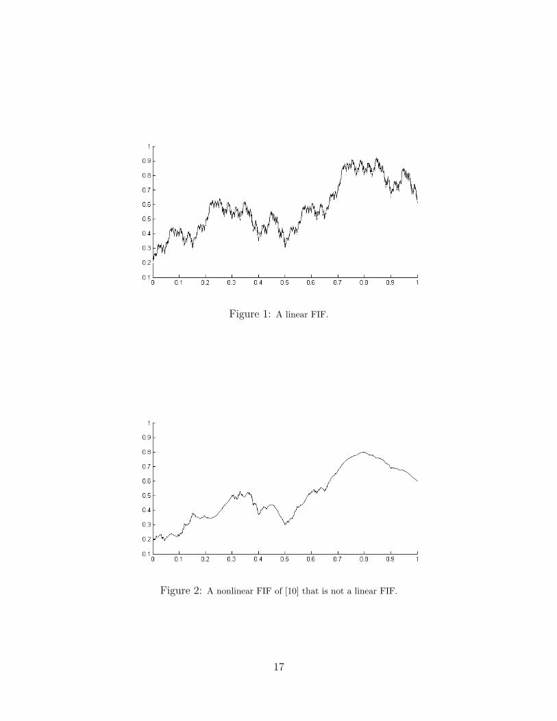
Figure 1: A linear FIF.
Figure 2: A nonlinear FIF of [10] that is not a linear FIF.
17
185

Figure 3: A generalized FIF that is not a FIF of [10].
References
[1] M. F. Barnsley. Fractal functions and interpolation. Constr. Approx., 2:303–329, 1986.
[2] M. F. Barnsley and P. R. Massopust. Bilinear fractal interpolation and box dimension.J. Approx. Theory, 192:362–378, 2015.
[3] Zhigang Feng, Yizhuo Feng, and Zhenyou Yuan. Fractal interpolation surfaces withfunction vertical scaling factors. Appl. Math. Lett., 25(11):1896–1900, 2012.
[4] J. Jachymski and I. Jozwik. Nonlinear contractive conditions: a comparison and relatedproblems. Banach Center Publ., 77:123–146, 2007.
[5] G. G. Lukawska and J. Jachymski. The Hutchinson-Barnsley theory for infinite iteratedfunction systems. Bull. Aust. Math. Soc., 72:441–454, 2005.
[6] P. R. Massopust. Fractal functions, fractal surfaces and wavelets. Academic Press, SanDiego, 1994.
[7] E. Rakotch. A note on contractive mappings. Proc. Amer. Math. Soc., 13:459–465,1962.
[8] B. E. Rhoades. A comparison of various definitions of contractive mappings. Trans.Am. Math. Soc., 226:257–290, 1977.
[9] Song-il Ri. A new fixed point theorem in the fractal space. Indagationes Mathematicae,27(1):85–93, 2016.
18
186

[10] Songil Ri. A new nonlinear fractal interpolation function. Fractals, 25(6):1750063 (12pages), 2017.
[11] N.-A. Secelean. Generalized iterated function systems on the space l∞(X). J. Math.Anal. Appl., 410(2):847–858, 2014.
[12] Hong-Yong Wang and Jia-Shan Yu. Fractal interpolation functions with variable pa-rameters and their analytical properties. J. Approx. Theory., 175:1–18, 2013.
19
187

188

Hidden Bifurcation kind to Multiscroll ChaoticAttractors via Saturated Function Series
Zaamoune Faiza1 and Tidjani Menacer2
1 Department of Mathematics, University Mohamed Khider, Biskra, Algeria(E-mail: [email protected])
2 Department of Mathematics, University Mohamed Khider, Biskra, Algeria(E-mail: [email protected])
Abstract. In this paper, design Hidden Bifurcation kind to Multiscroll ChaoticAttractors via Saturated Function Series are reconnoitred. The idea was taken fromthe work Zaamoune, et al(2019) and the method introduced by Menacer, et al. (2016)for Chua multiscroll attractors. These idea (hidden bifurcation kind) depends on howyou appear the scrolls odd or even were the number of scrolls is even. We have studiedmany examples to prove this idea, mentioned that the number n of scrolls satisfiesn = p + q + 2 in LU , Chen et al (2004).Keywords: Hidden bifurcation, multiscroll chaotic attractor, saturated functionseries..
1 Introduction
It is well known that the method hidden attractor generating one-directional(1-D) -scroll has been studied in the last few years [1]-[3]-[4]. Since the methodwas presented by Leonov, et al [4] in the Chua attractor, they have proposedefficient technique for the numerical localization of the hidden attractors inone-directional dynamical systems. Hidden attractor has many applicationsin a real word like mechanics, electronics, chemistry, biology but the mostimportant in electronic circuits (hysteresis circuit, and saturated circuit). In2016, the auteur’s Menacer, et al changed the type of discrete parameters bypresented a generating multi-spirals, and this new method they called a ”hiddenbifurcation”, the cause of this name it’s has a change in the number of spirals.In this paper, we study design hidden bifurcation kind method in the attractorfor generating one-directional (1-D) -scroll by saturated function series. In 2004Chen, et al design and analysis of multi scroll chaotic attractors from saturatedfunction series [8], but we present a new idea in hidden bifurcation, where weknow that the role of method hidden bifurcation it’s a parametres control inthe number of spirals, her in this work p1 and q1 in function 12 it’s a bossed. Inthis article, we change the values of system Chen parameters 11 a, b ,c and d1we found a new attractor different about Chen attractor in [8], we change everytime the parameter ε in 0.55 to 1 and the parameters p1 and q1 and we notedthat it’s not only the parameter εcontrol in the appearance of numbers scrolls,the parameters p1 and q1 also control in appearance of numbers scrolls it’s anew idea. This paper is disposed of as follows : In Section 2, the analytical-numerical method for hidden attractor proposed by Leonov in [6],[7]. the modelof 1−D scroll chaotic attractors generated by saturated function series proposed
189

.In Section 3, the model of 1−D scroll chaotic attractors generated by saturatedfunction series proposed. In section 4 , the localization technique presented in[2] for hidden bifurcation in 1−D scroll chaotic attractors, we introduced theresults for a new idea. Finally, in Sec. 6, a terse conclusion is pictured.
2 Analytical-numerical procedure for attractorslocalization
Leonov et al. [6],[9], [10] found a procedure to discover numerically hiddenattractor for Chua attractor. The technique developed in [2], discovering hiddenbifurcations in the multispiral Chua attractor. To improv, this numericalmethod, consider a system with one-directional (1-D) -scroll
dx
dt= Px+ βΨ(κTx), x ∈ R3. (1)
were P is a constant (n× n) matrix,β, κ are constant n−dimensional vectors,T is a transposition operation, Ψ(ς) is a continuous piecewise-differentiablevector-function, and Ψ(0) = 0. Consider a coefficient of Harmonic linearizationk at like the matrix P0 as :
P0 = P + kβκT (2)
wich ±iω0 (ω0 > 0) eigenvalues the matrix P0 and the rest have negative realparts. Suppose that such k occurs. So, rewrite system 1 as.
dx
dt= P0x+ βϕ(κTx), (3)
were ϕ(ς) = Ψ(ς)−kς.We display a fixed sequence of functions ϕ0(ς), ϕ1(ς), · · · , ϕn(ς),that the function ϕ0(ς) is small, and ϕm(σ) = ϕ(ς). In this state the smallness offunction ϕ0(ς), permit one to practise the procedure of harmonic linearizationfor the system
dx
dt= P0x+ βϕ0(κTx) (4)
and conclude a stable nontrival periodic solution x0(t). So, the localization ofthe attractor of a system(19), design numerically the transformation of thisperiodic solution. So, we obtain the primary condition x0(0) of the periodicsolution, system (4) can be changed by S (X = SY ) to the form :
·y1 = −ω0y2 + v1ϕ
0(y1 + ct3Y3)·y2 = ω0y1 + v2ϕ
0(y1 + ct3Y3)·Y3 = A3Y3 + V3ϕ
0(y1 + ct3Y3)
(5)
So V3 and c3 is an (n− 2)−dimensional vector, y1, y2 are scalar values; Y3 isan (n− 2)−dimensional vector, v1 and bv2 are real numbers; A3 is an (n− 2)×(n− 2) matrix, where all of its eigenvalues have negative real parts. Supposedthat for the matrix A3 there exists a d3 > 0 such that
Y t3 (A3 +At3)Y3 ≤ −2d3 |Y3|2 , ∀Y3 ∈ Rn−2. (6)
190

In one-directional(1-D) -scroll, case, present the describing function Φ of a realvariable ς as follows:
Φ (ς) =
∫ 2π/ω0
0
cos(ω0t)ς) cos((ω0t) dt (7)
Theorem 1. If a positive ς0 satisfies that
Φ(ς0) = 0, b1dΦ(ς)
dς
∣∣∣∣∣ς=ς0
< 0 (8)
So, for the initial condition of the periodic solution X0(0) = S(y1(0), y2(0),Y3(0))T at the first step of algorithm, one has
y1(0) = ς0 +O(ε), y2(0) = 0, Y3(0) = On−2(ε) (9)
In Application, to find k and ω0, can uses the transfer function of system (4),
W (ρ) = κT (M − ρI)−1β (10)
where ρ is a complex variable. The number ω0 is calculated from the equationImW (iω0) = 0 and k is then determined using the formula k0 = −ReW (iω0).
3 1 − D Scroll Chaotic Attractor via a saturatedfunction series
Here, to generate 1−D n scroll chaotic attractor we presented a system fromsaturated function series follows :
·x = y·y = z·z = −ax− by − cz + d1f(x; k1;h1; p1; q1)
(11)
where
f(x; k1;h1; p1; q1) =
y1 if x > q1h1 + 1y2 if |x− ih1 ≤ 1,−p1 ≤1 i ≤ q1|y3 if ih1 + 1 < x < (i+ 1)h1 − 1and − p1 < i < q1 − 1y4 if x < −q1h1 − 1
(12)
y1 = (2q1 + 1) k1 , y2 = k1 (x− ih1) + 2ik1, y3 = (2i+ 1) k1, and y4 =− (2q1 + 1) k1here, a, b, c, d1 are real numbers and the parameters p1, q1, h andk are integers. The formula to calculated the number n of scrolls, it’s explainedin Chen, et al [8] and in Zaamoune, et al[11] For k = 11,h = 22,p1 = 3, q1 = 3,a = d1 = 0.8, c = 0.72 and b = 0.6 a 8-scroll attractor is generated as theverged attractor of the system (11-12), see Fig 1
191
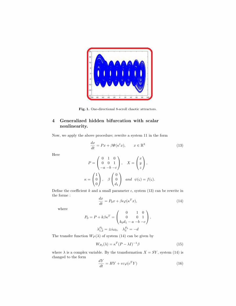
Fig. 1. One-directional 8-scroll chaotic attractors.
4 Generalized hidden bifurcation with scalarnonlinearity.
Now, we apply the above procedure; rewrite a system 11 in the form
dx
dt= Px+ βΨ(κtx), x ∈ R3 (13)
Here
P =
0 1 00 0 1−a −b −c
, X =
xyz
,
κ =
100
, β
00d1
and ψ(ς) = f(ς).
Define the coefficient k and a small parameter ε, system (13) can be rewrite inthe forme :
dx
dt= P0x+ βεϕ(κTx), (14)
where
P0 = P + kβκT =
0 1 00 0 1
k0d1 − a −b −c
,
λP01,2 = ±iω0, λP0
3 = −d
The transfer function WP (λ) of system (14) can be given by
WP0(λ) = κT (P − λI)−1β (15)
where λ is a complex variable. By the transformation X = SY , system (14) ischanged to the form
dY
dt= HY + vεϕ(cTY ) (16)
192

where
H =
0 −ω0 0ω0 0 00 0 −d
, Y =
y1y2Y3
, v =
v1v21
and c =
10−h
. The transfer function of system (16) can be written as
WH(λ) = cT (H − Iλ)−1v= h
d+λ − λv1
λ2+ω20
+ ω0v2
λ2+ω20
So, we could obtain the implies k, d, h, v1, v2 by using the equality of transferfunctions of systems (14) and (16):
WH(λ) = κT (M0 − λI)−1β (17)
This implies the following relations:
k0 =a−ω2
0dd1
d = c
h = −d1ω2
0+d2
v1 = −d1ω2
0+d2
v2 = −cd1ω0(ω2
0+d2)
(18)
We utilized the transformation X = SY the following relationships can begotten :
H = S−1P0S, b = S−1β, cT = κtS (19)
So, by 19 we found this matrix :
S =
S11 = 1 S12 = 0 S13 = −hS21 = 0 S22 = −ω0 S23 = dh
S31 = −ω30 S32 = 0 S33 = d2h
So, thr first step in above procedure is determine the initial data, as
X(0) = SY (0) = S
ς000
=
ς0S11
ς0S21
ς0S31
(20)
For system the Chen, the initial condition is :
X0(0) =
(x0(0) = ς0, y
0(0) = 0, z0(0) = −ς0ω30
)(21)
193
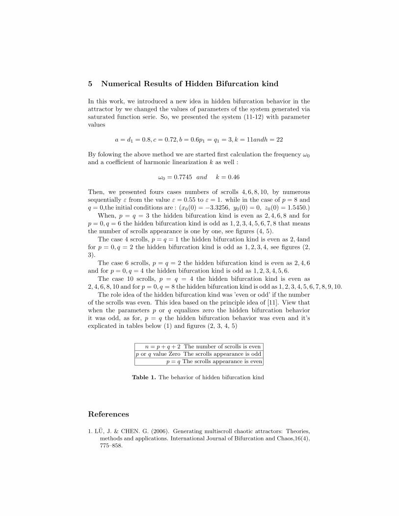
5 Numerical Results of Hidden Bifurcation kind
In this work, we introduced a new idea in hidden bifurcation behavior in theattractor by we changed the values of parameters of the system generated viasaturated function serie. So, we presented the system (11-12) with parametervalues
a = d1 = 0.8, c = 0.72, b = 0.6p1 = q1 = 3, k = 11andh = 22
By folowing the above method we are started first calculation the frequency ω0
and a coefficient of harmonic linearization k as well :
ω0 = 0.7745 and k = 0.46
Then, we presented fours cases numbers of scrolls 4, 6, 8, 10, by numeroussequentially ε from the value ε = 0.55 to ε = 1. while in the case of p = 8 andq = 0,the initial conditions are : (x0(0) = −3.3256, y0(0) = 0, z0(0) = 1.5450.)
When, p = q = 3 the hidden bifurcation kind is even as 2, 4, 6, 8 and forp = 0, q = 6 the hidden bifurcation kind is odd as 1, 2, 3, 4, 5, 6, 7, 8 that meansthe number of scrolls appearance is one by one, see figures (4, 5).
The case 4 scrolls, p = q = 1 the hidden bifurcation kind is even as 2, 4andfor p = 0, q = 2 the hidden bifurcation kind is odd as 1, 2, 3, 4, see figures (2,3).
The case 6 scrolls, p = q = 2 the hidden bifurcation kind is even as 2, 4, 6and for p = 0, q = 4 the hidden bifurcation kind is odd as 1, 2, 3, 4, 5, 6.
The case 10 scrolls, p = q = 4 the hidden bifurcation kind is even as2, 4, 6, 8, 10 and for p = 0, q = 8 the hidden bifurcation kind is odd as 1, 2, 3, 4, 5, 6, 7, 8, 9, 10.
The role idea of the hidden bifurcation kind was ’even or odd’ if the numberof the scrolls was even. This idea based on the principle idea of [11]. View thatwhen the parameters p or q equalizes zero the hidden bifurcation behaviorit was odd, as for, p = q the hidden bifurcation behavior was even and it’sexplicated in tables below (1) and figures (2, 3, 4, 5)
n = p + q + 2 The number of scrolls is even
p or q value Zero The scrolls appearance is odd
p = q The scrolls appearance is even
Table 1. The behavior of hidden bifurcation kind
References
1. LU, J. & CHEN. G. (2006). Generating multiscroll chaotic attractors: Theories,methods and applications. International Journal of Bifurcation and Chaos,16(4),775–858.
194

2. MENACER, T., LOZI, R. & CHUA, L.O. (2016). Hidden bifurcations in themultispiral Chua attractor. International Journal of Bifurcation and Chaos,16(4),1630039–1630065.
3. KUZNETSOV, N. V., LEONOV, G. A. & PRASAD, A. (2016). Hidden attractorsin dynamical systems. Physics Reports, 637, 1-50.
4. DENG, Q. & WANG, C. (2019). Multi-scroll hidden attractors with two stableequilibrium points. Chaos 29, 093112. https://doi.org/10.1063/1.5116732
5. ZHANG, X., & WANG C. (2019), Multiscroll Hyperchaotic System with HiddenAttractors and Its Circuit Implementation. International Journal of Bifurcationand Chaos, 29 (09), 1950117.
6. LEONOV, G. A., & KUZNETSOV, N. V. (2011). Localization of hidden Chua’sattractors. Phys. Lett. A, 375, 2230–2233.
7. LEONOV, G. A. (2010). Effective methods for periodic oscillations search indynamical systems. Appl. Math. Mech, 74, 37–73.
8. LU, J., CHEN, G. YU, X & LEUNG, H. (2004). Design and analysis of multiscrollchaotic attractors from saturated function series. IEEE Trans. Circuits Syst. I,51(12), 2476–2490.
9. LEONOV, G. A. VAGAITAEV, V. I. & KUZNETSOV, N. V. (2010). Algorithmfor localizing Chua attractors based on the harmonic linearization method. Dokl.Math, D, 663–666.
10. LEONOV, G. A., KUZNETSOV, N. V. (2013). Hidden attractors in dynamicalsystems. From hidden oscillations in Hilbert–Kolmogrov, Aizerman, and Kalmanproblems to hidden chaotic attractor in Chua circuits International Journal ofBifurcation and Chaos, 23, 1330002-1–1330002-69.
11. Zaamoune, F. T. Menacer, R. Lozi. & Chen, G. (2019). Symmetries in HiddenBifurcation Routes to Multiscroll Chaotic Attractors Generated by SaturatedFunction Series. Journal of Advanced Engineering and Computation, 3,4,511–522.
195

(a) (b)
(c)
Fig. 2. The increasing number of spirals of system (14) according to increasing εvalues, when p = 1 and q = 1, k=11 and h=22. (a) : The first scroll for ε=0.55, (b): The second scroll for ε=0.92, (c) : The third scroll for ε=1.
196

(a) (b)
(c)
Fig. 3. The increasing number of spirals of system (14) according to increasing εvalues, when p = 2 and q = 0, k=11 and h=22. (a) : The first scroll for ε=0.55, (b): The second scroll for ε=0.92, (c) : The third scroll for ε=1.
197

(a) (b)
(c) (d)
Fig. 4. The increasing number of spirals of system (14) according to increasing εvalues, when p = 3 and q = 3, k=11 and h=22. (a) : The first scroll for ε=0.55, (b): The second scroll for ε=0.92, (c) : The third scroll for ε=0.975, (d) : The last scrollfor ε=1
198

(a) (b)
(c) (d)
(e) (f)
(g)
Fig. 5. The increasing number of spirals of system (14) according to increasing εvalues, when p = 6 and q = 0, k=11 and h=22. (a) : The first scroll for ε=0.55, (b) :The second scroll for ε=0.92, (c) : The third scroll for ε=0.98, (d) : The fourth scrollfor ε=0.985, (e) : The fifthly scroll for ε=0.99, (f) : The sixthly scroll for ε=0.992,(g) : The last scroll for ε=1
199

200

Analysis of thermal and quantum escape timesof Josephson junctions for signal detection
G. Filatrella1, C. Barone2, C. Guarcello3, A. S. Piedjou Komnang3, V.Pierro4, A. Rettaroli5, and S. Pagano2
1 INFN Gruppo Collegato Salerno and Dept. of Sciences and Technologies, Univ. ofSannio, Via F. De Sanctis, I-82100 Benevento, Italy(E-mail: [email protected])
2 INFN, Gruppo Collegato Salerno and Dept. of Physics, Univ. of Salerno, ViaGiovanni Paolo II, I-84084 Fisciano (SA), Italy
3 Dept. of Physics, Univ. of Salerno, Via Giovanni Paolo II, I-84084 Fisciano (SA),Italy
4 INFN Gruppo Collegato Salerno and Dept. of Engineering, University of Sannio,Corso Garibaldi 107, I-82100 Benevento, Italy
5 INFN, Laboratori Nazionali di Frascati, Frascati (Roma) Italy and Dept. ofMathematics and Physics, University of Roma Tre, I-00100 Roma, Italy
Abstract. In this work we investigate the limits to the possibility to reveal the exis-tence of weak microwave signals through Josephson junctions. Even if the Josephsonelement is capable to reveal the electromagnetic field, thermal noise is to be quantifiedby means of signal theory, as a confounding factor that limits the detection. We showhow the decision problem can be embedded in the frame of signal detection. As aconsequence, the optimization of the detection probability and the minimization ofthe false alarm probability give a guide to select the Josephson junction parametersthat best suit the purpose.Keywords: Josephson junctions, Escape time, Signal detection, Particle detection.
1 Introduction
When Josephson junctions (JJ) are employed as detectors of microwave signals,they can reach a very high response (of the order of kV/W [31]), close to thequantum sensitive limit [14,15,26]. Moreover, as superconducting elements, thedevices can work no matter how the temperature is lowered, thus allowing tominimize thermal noise, at least until the contribution to the escapes throughquantum tunneling processes becomes statistically dominant. These premisesare, in a nutshell, the basis for the intensity of the efforts devoted to thedevelopment of highly-sensitive detectors based on JJ [3], as well as Josephsoncalorimeters [35,16]. To reveal even very weak electromagnetic signals, theenergy to induce the transition between two states of the JJ should be close tothe single photon energy. As the interaction between the JJ and the signal isgenerally mediated by a resonant cavity, also the latter excitation should be onthe same energy scale [20]. Thus, for a more detailed description of the devicepotentialities and limits, it is necessary to embed the problem in the context ofmicrowave photon manipulation through superconducting electronics [13,1]. Indoing so, the energy landscape of the device, as well as the antenna interaction
201

with the microwave photon field, are essential for a device description [4]. Itis in fact the JJ potential that dictates the disturbing switches due to thermalescapes and quantum tunneling [4,32]. A model for the detector consists of acurrent drive that perturbs the JJ dynamics and favors the switches to a finitevoltage state; the statistics of the escape times are analyzed to highlight thepresence of the perturbation.
Several remarkable achievements have been reached so far. The minimumphoton content that can be revealed through JJ has been estimated in the orderof 102, a limit that can be possibly lowered [36]. It has also been demonstratedthat it is possible to resolve the number of photons in a propagating mode [11].Quite naturally, to decide about the presence of a weak signal, it is necessary toachieve a silent enough state, that is a device capable to stay quite if no signalis applied. Some schemes that exploit the phase diffusion regime have beenrecently proposed with such purpose [30]. However, for the purpose to exploitthe high sensitivity of JJ in the search for photons resulting from elusive parti-cles as axions [7–9,28,10,22,37,3], it is necessary to set up a different detectionscheme to ascertain the existence of extra photons, above and beside the back-ground [5]. The purpose of this work is to analyze a scheme for the detectionof such excess photons through the analysis of the JJ switching currents [2,29],embedded in the frame of signal detection [12]. In fact, as the Josephson phaseis of quantum nature it is not directly accessible, detection is possible only ifthe photons cause a switch, a passage from the superconducting state to a fi-nite voltage state (mathematically, the problem amounts to determine the firstpassage time across the separatrix of a potential well [17]). As the passage alsooccurs because of thermal fluctuations, a careful analysis is necessary to provethat the passages are a consequence of some external field. The framework ofsignal detection allows to make simple estimates of the temperature constraintsand of the experimental set-up. As a consequence, the optimization of the de-tection probability (and the minimization of the false alarm probability) givesa guide to select the JJ parameters that best suit to reveal weak microwavesignals. In brief, detection amounts to the following question: how is it possibleto infer the presence of microwave extra photons, apart the thermal ones, fromthe analysis of the switches to the finite voltage of a JJ? A tentative answer tothis question is the subject of the present paper, organized as follows: in Sect.2 the problem will be extensively formulated, alongside with the description ofan electrical model for the dynamics of a JJ and of a perturbation. In Sect.3 the signal analysis indications for the performances of the detection will berecounted. Last Sect. 4 concludes.
2 The problem
We shall consider a small tunnel JJ coupled to the environment through thebias current:
C~2e
d2ϕ
dt′2+
1
R
~2e
dϕ
dt′+ I0 sinϕ = Ib + IN (t′) + IS(t′) (1)
202

The right hand side of this equation summarizes the current supplied to thejunction. In this formulation, therefore, one assumes that the impedance ofthe Josephson element is much lower than the impedance of any source, andconsequently the external world is seen as a current source (although otherconfigurations are possible, in which a voltage bias is more appropriated [24]).Eq. (1) includes inertia (determined by the capacitance C), dissipation (asgoverned by the dissipative element R) and fluctuations (the random currentIN (t′) supplied by the resistance), the nonlinear periodic term (the oscillatingJosephson current of amplitude I0), a constant bias current Ib, and the signalcurrent IS(t) (that summarizes the effects of the photon field). Fluctuationsare assumed to be Gaussian with:
〈IN (t′)〉 = 0, (2)
〈IN (t′)IN (t′ − s′)〉 =2kBT
Rδ(t′ − s′). (3)
where kB is the Boltzmann constant, T is the absolute temperature, δ the Diracfunction, 〈·〉 is the expectation operator.
The usual normalized units [6,33] are as follows (here, as usual, ~ is thereduced Planck constant, and e is the elementary charge):
• The current is normalized to the critical current I0:
γ =IbI0. (4)
• Time is normalized to ω−1J , where ωJ =√
~C/2eI0 is the frequency of thelinear oscillator. :
t = t′ωJ . (5)
Introducing the normalized temperature D = kBTωJ
/RI20 and the normalized
conductance 1/βc = (1/R)
√~/
(2eI0C), leads to the normalized versions of
Eqs.(1,2,3):
d2ϕ
dt2+
1
βc
dϕ
dt+ sinϕ = γ + γN (t) + γS(t), (6)
〈γN (t)〉 = 0, (7)
〈γN (t)γN (t− s)〉 = 2Dδ(t− s), (8)
where γ’s indicate the normalized current terms. The dynamics of the JJ ischaracterized by the bias-dependent small oscillation frequency:
ω0(γ) =(1− γ2
)1/4(9)
and the energy barrier that cages the dynamics is:
∆U(γ) = 2[√
1− γ2 − γ cos−1(γ)]. (10)
Finally, the photon field γS is supposed to be modeled as a succession of nor-malized impulses of amplitude A and duration δτ that arrive regularly with aperiod T . The response of a JJ to such a field, and how the response can beexploited to infer the existence of the field, is the problem dealt with in thispaper. Some indications are presented in the next Section.
203

0 100 200 300 400 500
0
2 π
4 π
6 π
t
φ
0 100 200 300 400 5000
5
10
15
20
t
dφ/dt
t1 t2 t3 t1 t2 t3
Fig. 1. Time dependent dynamics of the phase ϕ and the voltage dϕ/dt. The dashedlines denote the time at which a passage to the finite voltage is detected.
3 Results
A JJ described by Eqs.(6,7,8) can undergo switches between the zero voltageand the finite voltage, as shown in Fig.1. When the system switches, thephase difference increases and, according to the a.c. Josephson relation V =(h/2e)dϕ/dt [18,19], a voltage drop across the junction can be measured. Theswitches can occur either because of thermal current (7,8), or because of thecurrent pulse train. The starting point is therefore to collect the sequence oftimes at which a passage has occurred in the absence of the photon field drive:
t01, t02, ... , t
0N . (11)
For this case, one expects that, on average, the escapes (the passages acrossthe separatrix between the localized oscillations and unbound runaways) occurwith a rate given by the Kramers approximation [17]:
r0(γ,D) =ω0
2πe−
∆U(γ)D (12)
(for the Gaussian noise; other kinds of noise give pretty different results [25]).In the presence of a signal, which mimic the absorption of some photons that
is capable to induce a current into the JJ, the sequence of switches is presumablyaltered, and the photons can be possibly revealed through deviations from thepurely thermal sequence (11); let us call the sequence of the escapes in thepresence of the extra-photons:
t11, t12, ... , t
1N . (13)
This sequence is expected to have a larger number of events in the same observa-tion time respect to the unperturbed case (11). An example of two histogramsfor t0 (no signal) and t1 (with signal) are shown in Fig. 2. We underlinethat, at variance with the cases in which one is interested in counting the num-ber of photons (e.g., [20]), to reveal a source of photons (e.g., the presence ofan axion field [3]) it suffices to statistically determine if an observed collectionof switches is more likely drawn from sequence (11) or from sequence (13).
204

Fig. 2. Histograms of N = 104 switching times. Parameters of the simulations are:γ = 0.8, D = 0.1, 1
/βc = 0.025. The impulses that mimic the photon fields are of
amplitude A = 0.5, duration δτ = 10, and arrive regularly with a period T = 100.
In the simplest approximation, one expects that the rate r1 associated tothe escapes (13) in the presence of photons is just the sum of the unperturbedrate r0 and an additional rate rA due to the photons:
r1(γ,D, γS) = r0(γ,D) + rA. (14)
In our settings, where the photons are modeled as current pulses with a periodT , we have rA = 1/T for a most efficient detector.
Apart the analytical approximations embodied in Eq.(14), for our line ofreasoning it is important to underline that the rates r0 and r1 are statisticalaverages, for Eqs.(12,14) predict what happens on average. Thus, in a givenmeasurement time P one expects 1
/〈t0i 〉 = n0 = Pr0 escapes in the purely
thermal case, and 1/〈t1i 〉 = n1 = Pr1 escapes in the presence of the extra
photons, with the obvious inequality n1 > n0. In an actual measurement, oneobserves a certain number of switches, say n, and a decision is to be made: inwhich sense the measured number favors an hypothesis (the switches are justdue to thermal activation) or the other (there are extra switches due to thephoton field)? Naturally, the more the two rates are apart, the more likelyis that the measurement is a clear cut decision. Also, no matter how closethey are, with a sufficiently long measurement time P it is always possibleto discriminate the two conditions. To make these ideas quantitative is theobjective of the next Section.
205

r ≡ r0 with rA = 10-3
r ≡ rA with r0 = 10-3
500 1000 1500 20000
1000
2000
3000
4000
5000
r-1
P
Fig. 3. Length of the observation period P , according to estimate (16), as a functionof rA at a fixed r0 = 0.001 (solid red curve) and as a function of r0 at a fixedrA = 0.001 (dashed blue curve).
3.1 Statistical analysis of the switching times
To quantify the efficiency of the detection of a photon field one can introduce theKumar-Caroll (KC) index dKC [21], in analogy with the detection of continuoussinusoidal signals [12,2]:
dKC =|〈t1〉 − 〈t0〉|√
12 [σ2(t1) + σ2(t0)]
. (15)
where 〈t0,1〉 is the average switching time in the absence (presence) of thesignal, and σ2(t0,1) the corresponding variances. This index is a proxy for theSignal-to-Noise-Ratio (SNR) [21], and as such will be used in this paper.
Assuming a large number of events in the measurement time P , and that theescapes due to the photons are an additional rate independent of the thermalrate, and that a reliable detection requires at least dKC = 1, one obtains therelation [34]:
P r2A −1
2rA − r0 = 0, (16)
between the rate of the photons rA, the thermal escape rate r0, and the obser-vation time P . Inspection of Eq.(16) reveals that the measurement time lengthP is positively related to the thermal rate r0, see Fig. 3.
Some further elaborations of the estimate (16) are relevant. To begin with,one can define a ratio between the photon arrivals and the thermal spontaneousescapes:
r0 = x rA
that allows to explicitly observe that:
dKC =
√2PrA2x+ 1
. (17)
206

500150035005000
0.1 0.5 1 5 100.001
1
10
rA × 10-3
r0×
10-
3P
0.01
0.1
Fig. 4. Relation between the thermal escape rate as a function of the photon arrivaltime, according to estimate (16), for different values of P .
This equation confirms the intuitive scaling between the observation time P ,the photon arrival rate, and the ratio between the thermal and photon rates.In particular, one can insert the matching condition P = 1/rA in Eq. (17) toobtain the relation between the observation time, the temperature and biaspoint through Eqs. (9)–(12).
In Fig. 3 it is displayed the behavior of the observation time P , calculatedaccording to Eq. (16), as a function of the inverse photon rate, r−1A (see the redsolid curve). If the photon rate is low, e.g. around 10−3 Hz, the observationtime for a dKC = 1 reads ∼ 1500 s. It is also noticeable that the dependenceis quadratic. Should the photon rate be much smaller than the assumed mHz,the detection could prove unfeasible. Conversely, if the photon arrival rate isrelatively high, one can considerably increase also the thermal rate, and hencehigher temperatures are allowed.
In Fig. 4 it is displayed the behavior of the thermal escape rate, r0, as afunction of the photon arrival time, rA, for different values of the observationtime P . It is evident that the thermal escape rate (that is, the temperature ofthe system) can be increased as the photon rate increases. However, for anyvalue of P , there is a threshold value of rA (e.g., rA ' 103 for P = 500) belowwhich thermal escapes to achieve a dKC = 1 become vanishingly small. Thelatter condition entails extremely low temperatures.
In brief, if some SNR is to be reached, the trade-off between the parametersof the experiment can be evaluated. A more detailed analysis of the problemrequires to retrieve the index (15) from numerical simulations of the modelequations (6,7,8), as we shall do below.
3.2 An example of the Kumar-Carrol index usage
To illustrate an application of the signal-to-noise index (15), let us supposethat the index has been computed for several values of the bias current γ tooptimize the bias level. To fix the ideas, let us suppose that the highest valueof dKC corresponds to γ = 0.8; the escapes retrieved for such choice are shown
207
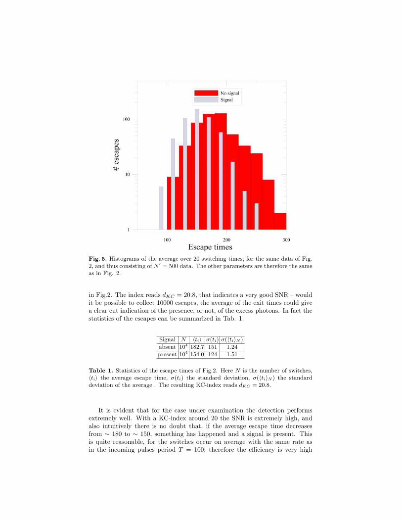
Fig. 5. Histograms of the average over 20 switching times, for the same data of Fig.2, and thus consisting of N ′ = 500 data. The other parameters are therefore the sameas in Fig. 2.
in Fig.2. The index reads dKC = 20.8, that indicates a very good SNR – wouldit be possible to collect 10000 escapes, the average of the exit times could givea clear cut indication of the presence, or not, of the excess photons. In fact thestatistics of the escapes can be summarized in Tab. 1.
Signal N 〈ti〉 σ(ti) σ(〈ti〉N )
absent 104 182.7 151 1.24
present 104 154.0 124 1.51
Table 1. Statistics of the escape times of Fig.2. Here N is the number of switches,〈ti〉 the average escape time, σ(ti) the standard deviation, σ(〈ti〉N ) the standarddeviation of the average . The resulting KC-index reads dKC = 20.8.
It is evident that for the case under examination the detection performsextremely well. With a KC-index around 20 the SNR is extremely high, andalso intuitively there is no doubt that, if the average escape time decreasesfrom ∼ 180 to ∼ 150, something has happened and a signal is present. Thisis quite reasonable, for the switches occur on average with the same rate asin the incoming pulses period T = 100; therefore the efficiency is very high
208

(almost each pulse causes a switch) and the number of data is conspicuous(N = 104). Under these circumstances, the statistical analysis is just a confirmof the intuition. However, the approach proves useful for the design of anexperiment if it is not possible to collect as many as 104 switches. Let ussuppose, ceteris paribus, that the rate of arrival of the pulses is extremely low,say 1
/rA ∼ 1h, and therefore the number of events that can be collected in a
day of measurements is around N = 20. A principal question would be: howmany days of data collection should be planned to decide, with good confidence,about the existence of the pulses?
Let us thus suppose that the actual sample of data to be analyzed consistsof M escape times, M N , say M = 20 to fix ideas. A collection of 500average escape times (over M = 20 events) retrieved binning the 104 data ofFig. 2, is shown in Fig. 5. In a single measurement run in which 20 switchesare collected, a single average escape time would be obtained, and not alwaysthe same value for the statistical fluctuations. Let us summarize the data inTab. 2.
Signal N ′ 〈ti〉 σ(ti) σ(〈ti〉N′)
absent 500 182.7 33.8 1.24
present 500 154.0 27.7 1.51
Table 2. Statistics of the escape times of Fig.5, that is the escape times averagedover M = 20 events. Here N ′ = N/M = 500 is the number of means, 〈ti〉 theaverage escape time over N ′ × M escapes, σ(ti) the standard deviation of the N ′
means, σ(〈ti〉N′) the standard deviation of the overall average. Naturally, 〈ti〉 andσ(〈ti〉N′) coincide with Table 1, as they are computed on the same set of data. Theresulting KC-index for a single measurement (that is, an average over 20 data) readsdKC = 0.93.
In the first place, let us remind of a subtle difference between Fig. 2 andFig. 5, as perhaps better explained in the corresponding Table 1 and Table 2.Figure 2 is a collection of all data, any single switch that has occurred. Figure5 is a collection of hypothetical repetition of the average over 20 switches. Thestatistical test to decide about the presence of the signal is to be performed onthe average over all data in the case of Fig. 2, and hence the very high SNR,compared to the test on a single event of Fig. 5, to which pertains a muchsmaller SNR.
For the central limit theorem one can assume that the distribution of theaverages is approximately Gaussian, centered on the population average (thatis estimated through the average of the N = 104 data) and with a standarddeviation which is smaller than the population standard deviation.
Applying the signal analysis means to determine the error of the first typeα and of the second type β when a decision on the existence of the photonfield is to be made, on the basis of the escape time average. Let us do so withthe help of the Gaussian approximation, that is to assume that the histogramof the average escape time of Fig. 5 is Gaussian distributed, as schematically
209

Fig. 6. Application of the detection scheme to the averaged data assumed to beGaussian distributed.
illustrated by Fig. 6. To decide between the hypothesis one usually places athreshold for the measured average escape time, 〈t〉th, see Fig. 6. The decisionwill favor the hypothesis “1” (the photon field is there) if the actual measuredtime is below the threshold, and obviously the complementary hypothesis (thereis no photon field) will be selected if the actual measured time is above. Thechoice of the threshold reflects on the decision errors: either the probabilityof false alarm (type I error α), or the probability of missing a signal (typeII error β). These features are combined in the so-called receiver operatorcharacteristic of the test statistic, that is, of the combination of the errorsα and β for each particular choice of the threshold. It is natural, if thereare not particular reasons to do otherwise, to choose the case α = β thatunequivocally individuates a threshold and hence the errors. The features ofthe detection can thus be obtained by a straightforward application of thecentral limit theorem with the data of histogram of Fig. 2: it suffices to noticethat the standard deviation σ (ti) that appears in the definition of dKC (15)is smaller of a factor ∼
√M ' 4.5, as it is confirmed by Tables 1,2. In this
manner one can connect the SNR estimated through dKC to the size of typeI and II errors, as illustrated in Fig. 7. In this figure, we show the dKC
index as a function of the sample size M (open circles and solid line). Fromeach estimated dKC index, according to the condition α = β, we can uniquelydetermine the size of the errors of the test (triangles), see Fig. 6. In the samefigure, the solid line displays the dKC behavior estimated assuming that thestandard deviations in Eq. (15) decrease as the square root of the number ofdata in a sample,
√M . It is clear that such behavior scales nicely for M N .
Therefore, if a sufficiently long simulation is available, it is possible to carefullydesign the experiment to achieve the desired error bound.
Let us summarize how it is possible to put to a good use the definitionof the SNR through the KC-index (15). First, it is useful to select the mostappropriated parameter values to achieve the best SNR; in the present case wehave supposed that the optimization of the SNR has given the best bias pointγ = 0.8. For such parameter, a consistent number of events has been collected,
210

N = 104. From the data so collected, it has been possible to determine thenumber of experiments that could suffice to achieve the desired level of error(type I and II, chosen to be identical).
Fig. 7. Application of the detection scheme to the averaged data assumed to beGaussian distributed. The circles (left axis) indicate the SNR ratio estimated by theindex dKC . The triangles (right axis) indicate the α = β level of the errors in thedetection through the sample average as a function of the number of switches Mof the average. The solid line is the estimate obtained assuming that the standarddeviations scale as the square root of the number of points N . The other parametersare the same as in Fig. 2.
4 Conclusions
We have demonstrated that the application of signal analysis to switching eventof a Josephson junction subject to a periodic train of current pulses can beused to carefully plan experiments devised to decide about the existence ofthe perturbation. If the pulse train is to be interpreted as a photon fieldthat irradiates the junction, this scheme can be applied to decide about theexistence of elusive particles [3]. In particular the scheme can be useful ifthe arrival frequency of the pulses is very low, and therefore it is particularlycumbersome to collect a large number of events to distinguish the signal fromthe external field from spontaneously, thermally activated, events. Under thesecircumstances, it is necessary to resort to statistical test. When this is the case,the SNR to be reached for a significant test is the guideline for an accurate
211

experiment design. As the estimate of the SNR calls for extensive simulations,both to optimize the parameters and to collect a statistically relevant numberof events, it is probably necessary to resort to parallel simulations, possiblywith CUDA architecture [27].
Let us add a word of caution. The analysis here presented is based on samplemean, detection can be improved with maximum likelihood estimators [2], thatexploit the full information content of the escape distribution. However, theanalytical estimate of the distribution of the escapes is a relatively complicatedproblem [23] to give a reliable solution for the estimate evaluation.
Acknowledgments
The authors wish to acknowledge financial support from Italian National Insti-tute for Nuclear Physics INFN through the Project SIMP and from Universityof Salerno through projects FARB17PAGAN, FARB19PAGAN.
References
1. B. Abdo, O. Jinka, N. T. Bronn, S. Olivadese and M. Brink. On-chipsingle-pump interferometric Josephson isolator for quantum measurements.arXiv:2006.01918v1, 2020.
2. P. Addesso, G. Filatrella and V. Pierro. Characterization of escape times of Joseph-son junctions for signal detection. Physical Review E, 85, 016708-01–10, 2012.
3. D. Alesini, D. Babusci, C. Barone et al. Status of the SIMP Project: Towardthe Single Microwave Photon Detection. Journal of Low Temperature Physics,199, 348–354, 2020; Development of a Josephson junction based single photonmicrowave detector for axion detection experiments. Journal of Physics: Con-ference Series, 1559, 012020-1–7, 2020.
4. D. V. Anghel, K. Kulikov, Y. M. Galperin and L. S. Kuzmin, Electromagnetic ra-diation detectors based on Josephson junctions: Effective Hamiltonian. PhysicalReview B, 101, 024511-1–10, 2020.
5. E. Aprile it et al. Observation of Excess Electronic Recoil Events in XENON1T.arXiv:2006.09721 [hep-ex] , 2020.
6. A. Barone and G. Paterno Physics and applications of the Josephson effect7. C. Beck, Testing axion physics in a Josephson junction environment. Modern
Physics Letters A 26, 2841-2852, 2011.8. C. Beck, Possible resonance effect of axionic dark matter in Josephson junctions.
Phys. Rev. Lett. 111, 231801, 2013.9. C. Beck, Axion mass estimates from resonant Josephson junctions. Physics of the
Dark Universe 7–8, 6-11, 2015.10. C. Beck, Cosmological flux noise and measured noise power spectra in SQUIDs.
Scientific Reports 6, 28275, 2016.11. R. Dassonneville, R. Assouly, T. Peronnin, P. Rouchon and B. Huard, Number-
resolved photocounter for propagating microwave mode. arXiv:2004.05114[quant-ph], 2020.
12. G. Filatrella and V. Pierro. Detection of noise-corrupted sinusoidal signals withJosephson junctions. Physical Review E, 82, 046712-1–9, 2010;
13. Xiu Gu, A. F. Kockum, A. Miranowicz, Yu. Liu and F. Nori, Microwave photonicswith superconducting quantum circuits. Physics Reports, 718–719, 1–102, 2017.
212

14. C. Guarcello, D. Valenti, B. Spagnolo, V. Pierro and G. Filatrella. Anomaloustransport effects on switching currents of graphene-based Josephson junctions.Nanotechnology, 28, 134001, 2017.
15. C. Guarcello, D. Valenti, B. Spagnolo, V. Pierro and G. Filatrella. Josephson-based Threshold Detector for Levy-Distributed Current Fluctuations. PhysicalReview Applied, 11, 044078-01-09, 2019.
16. C. Guarcello, A. Braggio, P. Solinas, G. P. Pepe, and F. Giazotto. Phys. Rev.Applied, 11, 054074, 2019.
17. P. Hanggi, P. Talkner and M. Borkovec. Reaction-rate theory: fifty years afterKramers. Review of Modern Physics. 62, 251-341, 1990.
18. B. Josephson. Possible new effects in superconductive tunnelling. Physics Letters,1, 251, 1962.
19. B. D. Josephson. The discovery of tunnelling supercurrents. Rev. Mod. Phys., 46,251, 1974.
20. B. Kubala, J. Ankerhold and A.D. Armour. Electronic and photonic count-ing statistics as probes of nonequilibrium quantum dynamics. New Journal ofPhysics, 22, 023010-1–10, 2020.
21. B.V.K.V Kumar and C.W. Carrol. Performances of Wigner distribution functionbased detection methods. Optical Engineer, 23, 732–737, 1984.
22. L. S. Kuzmin, A. S. Sobolev, C. Gatti, D. Di Gioacchino, N. Crescini, A. Gordeevaand E. Il’ichev. Single Photon Counter Based on a Josephson Junction at 14 GHzfor Searching Galactic Axions. IEEE Transactions on Applied Superconductivity,28, 1–5, 2018
23. B. Lindner. Moments of the First Passage Time under External Driving. Journalof Statistical Physics, 117, 703–737, 2004.
24. M. Nashaat, A. E. Botha, and Yu. M. Shukrinov. “Devil’s staircases in the IVcharacteristics of superconductor/ferromagnet/superconductor Josephson junc-tions”, Phys. Rev. B 97, 224514 (2018).
25. V. V Palyulin, G. Blackburn, M. A. Lomholt, N. W. Watkins, R. Metzler, R.Klages and A. V. Chechkin. First passage and first hitting times of Lvy flightsand Levy walks. New Journal of Physics, 21, 103028, 2019.
26. F. Paolucci, N. Ligato, V. Buccheri, G. Germanese, P. Virtanen, and F. Gia-zotto. Hypersensitive tunable Josephson escape sensor for gigahertz astronomy.arXiv:2003.05966v2, 2020.
27. V. Pierro, L. Troiano, E. Mejuto and G. Filatrella. Stochastic first passage timeaccelerated with CUDA. Journal of Computational Physics, 361, 136–149, 2018.
28. V.A. Popov, Resonance detection of dark matter axions using a dc SQUID. Jour-nal of Experimental and Theoretical Physics 122, 236242, 2016.
29. O. V. Pountougnigni, R. Yamapi , C. Tchawoua, V. Pierro and G. Filatrella.Detection of signals in presence of noise through Josephson junction switchingcurrents. Physical Review E 101, 052205-1–10, 2020.
30. L. S. Revin, Andrey L. Pankratov, A. V. Gordeeva, A. A. Yablokov, I. V. Rakut,V. O. Zbrozhek and L. S. Kuzmin. Microwave photon detection by an Al Joseph-son junction. Beilstein Journal of Nanotechnology, 11, 960965, 2020.
31. S. J. Rezvani, D. Di Gioacchino, C. Gatti, C. Ligi, M. Cestelli Guidi, S. Cibella,M. Fretto, N. Poccia, S. Lupi and A. Marcelli. Proximity Array Device: A NovelPhoton Detector Working in Long Wavelengths. Condensed Matter, 5, 33-1–9,2020.
32. A. M. Sokolov and F. K. Wilhelm, A superconducting detector that counts mi-crowave photons up to two, arXiv:2003.04625v1, 2020.
33. F. Tafuri (Ed.) Fundamentals and Frontiers of the Josephson Effect, SpringerSeries in Materials Science, Volume 286, 2019.
213

34. SIMP collaboration. Analysis of Josephson junctions switching current distribu-tions for the optimal detection of microwave single photons. Presented at theErice meeting New trends in nonequilibrium stochastic multistable systems andmemristors. Ocotober 18-21, 2019, Italy.
35. E. D. Walsh, D. K. Efetov, G. Lee, M. Heuck, J. Crossno, T. A. Ohki, P. Kim,D. Englund and K. Chung. Graphene-Based Josephson-Junction Single-PhotonDetector, Physical Review Applied, 8, 024022-1–11, 2017.
36. A .A . Yablokov , V.M. Mylnikov, A.L. Pankratov, E.V. Pankratova and A.V.Gordeeva. Suppression of switching errors in weakly damped Josephson junctions,Chaos, Solitons and Fractals, 136, 109817-1–6, 2020.
37. J. Yan, C. Beck. Nonlinear dynamics of coupled axion–Josephson junction sys-tems. Physica D: Nonlinear Phenomena 403, 132294, 2020.
214
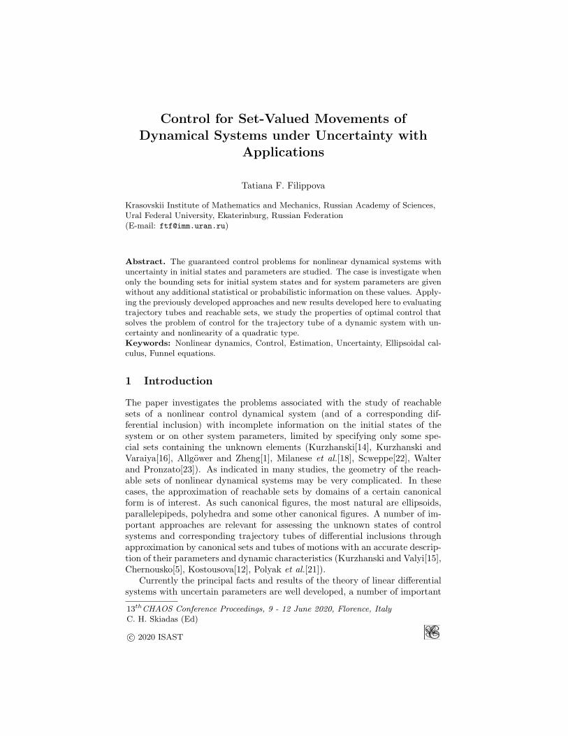
Control for Set-Valued Movements ofDynamical Systems under Uncertainty with
Applications
Tatiana F. Filippova
Krasovskii Institute of Mathematics and Mechanics, Russian Academy of Sciences,Ural Federal University, Ekaterinburg, Russian Federation(E-mail: [email protected])
Abstract. The guaranteed control problems for nonlinear dynamical systems withuncertainty in initial states and parameters are studied. The case is investigate whenonly the bounding sets for initial system states and for system parameters are givenwithout any additional statistical or probabilistic information on these values. Apply-ing the previously developed approaches and new results developed here to evaluatingtrajectory tubes and reachable sets, we study the properties of optimal control thatsolves the problem of control for the trajectory tube of a dynamic system with un-certainty and nonlinearity of a quadratic type.Keywords: Nonlinear dynamics, Control, Estimation, Uncertainty, Ellipsoidal cal-culus, Funnel equations.
1 Introduction
The paper investigates the problems associated with the study of reachablesets of a nonlinear control dynamical system (and of a corresponding dif-ferential inclusion) with incomplete information on the initial states of thesystem or on other system parameters, limited by specifying only some spe-cial sets containing the unknown elements (Kurzhanski[14], Kurzhanski andVaraiya[16], Allgower and Zheng[1], Milanese et al.[18], Scweppe[22], Walterand Pronzato[23]). As indicated in many studies, the geometry of the reach-able sets of nonlinear dynamical systems may be very complicated. In thesecases, the approximation of reachable sets by domains of a certain canonicalform is of interest. As such canonical figures, the most natural are ellipsoids,parallelepipeds, polyhedra and some other canonical figures. A number of im-portant approaches are relevant for assessing the unknown states of controlsystems and corresponding trajectory tubes of differential inclusions throughapproximation by canonical sets and tubes of motions with an accurate descrip-tion of their parameters and dynamic characteristics (Kurzhanski and Valyi[15],Chernousko[5], Kostousova[12], Polyak et al.[21]).
Currently the principal facts and results of the theory of linear differentialsystems with uncertain parameters are well developed, a number of important
13thCHAOS Conference Proceedings, 9 - 12 June 2020, Florence, ItalyC. H. Skiadas (Ed)
c© 2020 ISAST
215

and computationally useful algorithms have been constructed for finding theexternal and internal (with respect to the inclusion of sets) approximationsof the set-valued states of dynamical systems in the case of a linear systemdynamics. However the presence of nonlinear terms in the state velocities ofthe control systems causes a loss of the convexity of the reachable sets and,therefore, raises many theoretical questions and therefore requires the devel-opment of related mathematical tools and algorithms that are adequate tothe indicated problems of nonlinear analysis. Some ideas and approaches tothe study of set-valued motions (trajectory tubes) for a number of differentialsystems with nonlinearity and uncertainty in dynamics were presented earlierin Filippova[7], Filippova and Lisin[8], Filippova and Matviychuk[9] (see alsoreferences in the indicated publications).
In this paper we assume that in a dynamic system there are two types ofnonlinearity, namely, we have a combination of bilinear and quadratic func-tions in the state velocities. Earlier, we examined the problems of evaluatingthe reachable sets of systems under study taking into account all possible con-trols at once. Knowing the areas of reachability with respect to all parametersof the system under study (for all possible initial states, disturbances, controls)is very useful, since it helps to evaluate the capabilities of the system. However,it seems important to have a description of the trajectory tube generated by aspecific choice of a control function, it will allow solving optimization problemsfor set-valued movements of the considered systems under uncertainty. Notethat in this paper we consider a special class of control systems with nonlin-earity and uncertainty under other informational assumptions than was donein a recent paper Filippova and Matviychuk[10]. Thus, this research continuesand complements developments in the field of mathematical control theory re-lated to the study of the dynamics of multivalued states of nonlinear controlsystems. The approaches and algorithms presented here may be applied in thestudy of models with nonlinearity and uncertainty in real systems in robotics,economics, biology and other fields (considered e.g. in Allgower and Zheng[1],Bayen and Rapoport[2], Cecarelli et al.[4], Keller et al.[11]).
2 Problem formulation
2.1 Basic notations
The main notations used in the paper are basic; however, we define here someadditional, most frequently used and important constructions.
We denote by Rn the n-dimensional vector space and by compRn the setof all compact subsets of Rn. Also Rn×m denotes the set of all n×m-matrices.
The usual inner product of x, y ∈ Rn is x′y = (x, y) =∑ni=1 xiyi with prime
as a transpose and also the
‖x‖ = ‖x‖2 = (x′x)1/2, ‖x‖∞ = max1≤i≤n
|xi|
are corresponding norms for x ∈ Rn.
216
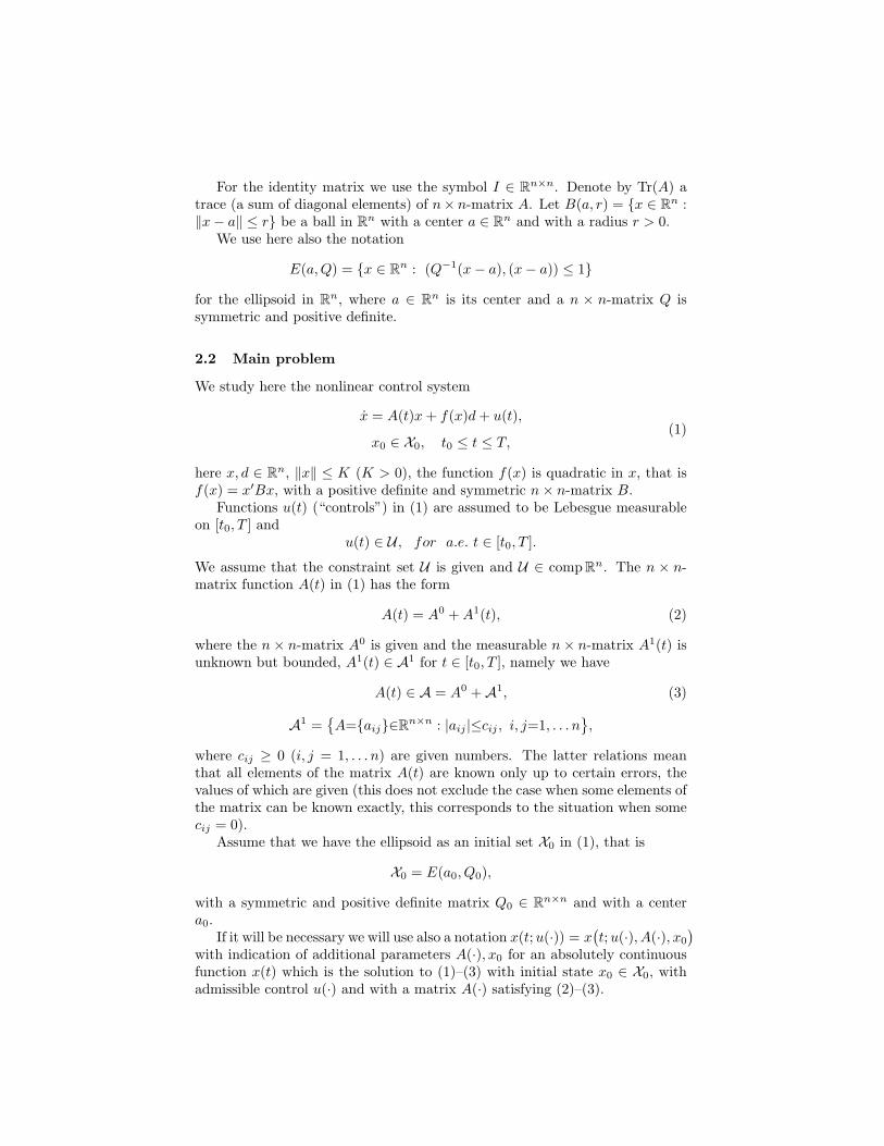
For the identity matrix we use the symbol I ∈ Rn×n. Denote by Tr(A) atrace (a sum of diagonal elements) of n× n-matrix A. Let B(a, r) = x ∈ Rn :‖x− a‖ ≤ r be a ball in Rn with a center a ∈ Rn and with a radius r > 0.
We use here also the notation
E(a,Q) = x ∈ Rn : (Q−1(x− a), (x− a)) ≤ 1
for the ellipsoid in Rn, where a ∈ Rn is its center and a n × n-matrix Q issymmetric and positive definite.
2.2 Main problem
We study here the nonlinear control system
x = A(t)x+ f(x)d+ u(t),
x0 ∈ X0, t0 ≤ t ≤ T,(1)
here x, d ∈ Rn, ‖x‖ ≤ K (K > 0), the function f(x) is quadratic in x, that isf(x) = x′Bx, with a positive definite and symmetric n× n-matrix B.
Functions u(t) (“controls”) in (1) are assumed to be Lebesgue measurableon [t0, T ] and
u(t) ∈ U , for a.e. t ∈ [t0, T ].
We assume that the constraint set U is given and U ∈ compRn. The n × n-matrix function A(t) in (1) has the form
A(t) = A0 +A1(t), (2)
where the n× n-matrix A0 is given and the measurable n× n-matrix A1(t) isunknown but bounded, A1(t) ∈ A1 for t ∈ [t0, T ], namely we have
A(t) ∈ A = A0 +A1, (3)
A1 =A=aij∈Rn×n : |aij |≤cij , i, j=1, . . . n
,
where cij ≥ 0 (i, j = 1, . . . n) are given numbers. The latter relations meanthat all elements of the matrix A(t) are known only up to certain errors, thevalues of which are given (this does not exclude the case when some elements ofthe matrix can be known exactly, this corresponds to the situation when somecij = 0).
Assume that we have the ellipsoid as an initial set X0 in (1), that is
X0 = E(a0, Q0),
with a symmetric and positive definite matrix Q0 ∈ Rn×n and with a centera0.
If it will be necessary we will use also a notation x(t;u(·)) = x(t;u(·), A(·), x0
)with indication of additional parameters A(·), x0 for an absolutely continuousfunction x(t) which is the solution to (1)–(3) with initial state x0 ∈ X0, withadmissible control u(·) and with a matrix A(·) satisfying (2)–(3).
217

Due to the fact that some quantities are unknown but bounded, we areforced to consider all possible versions of motions compatible with additionaldata as a generalized solution to the control system, that is, we need to replacea single-valued trajectory by a bundle or tube of motions of the following formX (t;u(·)).
Definition 1. For each admissible control u(·) the generalized solution tubeX (t;u(·)) (with t ∈ [t0, T ]) of system (1)–(3) is defined as follows,
X (t;u(·)) = x ∈ Rn :∃x0∈X0, ∃A(·)∈A,
x = x(t) = x(t;u(·), A(·), x0
).
Let us consider the following main problems.
Problem 1. For each feasible control u(·)∈U , find the optimal external ellip-soidal estimate E(a, Q;T, u(·)) of the reachable set X(T ;u(·)) of the system (1)-(4), such that
X (T ;u(·)) ⊂ E(a, Q;T, u(·)).
Remark 1. Here we understand the optimality of the desired ellipsoidal esti-mate, bearing in mind the closest operation with respect to inclusion of relatedsets.
Problem 2. Given a vector x∗ ∈ Rn find the feasible control u∗(·) ∈ U suchthat the related ellipsoidal estimate is optimal, that is we have
d(x∗, E(a∗, Q∗;T, u∗(·))) = infu(·)∈U
d(x∗, E(a∗, Q∗;T, u(·))) = ε∗.
3 Main results
First, we define an auxiliary parameter k, which is required to formulate themain result (see also Filippova[7]). To do this, consider the matrix B1/2Q0B
1/2
and denote its maximal eigenvalue as k2, that is we have
E(a0, Q0) ⊆ E(a0, (k+0 )2B−1), (4)
and k+0 is the smallest positive number for which this estimate (4) is true.
Theorem 1. The upper ellipsoidal estimate is true
X (t0 + σ;u(·)) ⊆ E(a∗(t0 + σ), Q∗(t0 + σ) | u(·)) + o(σ)B(0, 1) (5)
with σ−1o(σ)→ 0 for σ → +0 and
a∗(t0 + σ) = a(t0 + σ) + σ(a+ a′0Ba0 · d+ k2d) + σu(t0), (6)
and with functions a(t), Q∗(t) satisfying the following equations
˙a = A0a, t0 ≤ t ≤ T, a(t0) = a0, (7)
218

Q∗ = A0Q∗ +Q∗(A0)′ + qQ∗ + q−1G, Q∗(t0) = Q0, t0 ≤ t ≤ T, (8)
whereA0 = A0 + 2d · a′0B, q =
(n−1 Tr ((Q∗)−1G)
)1/2, (9)
G = diag
(n− v)[ n∑i=1
cji|ai|+(
maxσ=σij
n∑p,q=1
Q∗pqcjpcjqσjpσjq)1/2]2
, (10)
with a maximum in (10) calculated over numbers σij = ±1, i, j = 1, . . . , n,such that we have cij 6= 0 and v is a number of such indices i for which cij = 0for all j = 1, . . . , n.
Proof. The relation (5) is established along the main lines and ideas presentedin Filippova[7]. Indeed, from the funnel equation Panasyuk[20] we have
X(t0 + σ;u(·)) ⊆⋃
x∈E(0,k+02B−1)
(a0 + x+ σ(A0 +A1)(a0+
x) + σ(a0 + x)′B(a0 + x)) + σu(t0) + o(σ)B(0, 1). (11)
We remind that we may use here the property that at the boundary points xof the ellipsoid E(0, (k+0 )2B−1) we have the equality x′Bx = (k+0 )2 (for a moresimple case detailed explanations of the last property may be found also inFilippova[7]). With this property and rearranging the terms in (11), we cometo the formulas (5)-(10).
Remark 2. We see here that the ellipsoidal estimates of the tube X(t;u(·)) foreach fixed control u(·) are under investigation here and therefore the parametersof the estimation procedures depend on u(·). We can complicate the problemby additionally assuming the presence of state constraints or by considering aslightly more general class of uncertainty, e.g. in the coefficients of the matrixof linear terms of the state velocities.
Remark 3. It follows from Theorem 1 that we can construct a discrete tubeE(a, Q;T, u(·)) with ellipsoidal cross-sections that solves Problem 1 and forwhich we have the inclusion
X(T ;u(·)) ⊆ E(a+(T ), Q+(T );u(·)) + o(ε)B(0, 1). (12)
We emphasize that this discrete construction may be used as a basis for relatedcomputational schemes and algorithms allowing to find the trajectory tubesnumerically.
Using the results Filippova and Matviychuk[9], we may derive the followingresult.
Theorem 2. Let ε∗, u∗(·) be the optimal values of the Problem 2. Then wehave the relations
ε∗ = minu(·)∈U
max||l||=1
r+(T ;u(·))(l′B−1l)1/2+
l′(a+(T ;u(·))− x∗) = max||l||=1
r+(T ;u∗(·))(l′B−1l)1/2+ (13)
l′(a+(T ;u∗(·))− x∗).
219

Proof. First, we find the minimal positive number ε such that the followinginclusion is true
E(a+(T ), Q+(T );T, u(·)) ⊆ B(x∗, ε),
or equivalently
ρ(l|E(a+(T ), Q+(T );T, u(·)) ≤ ρ(l|B(x∗, ε)), ∀l ∈ Rn.
Appling the result of Theorem 1, we get the relation
l′a+(T ) + (l′Q+(T )l)1/2 ≤ l′x∗ + ε||l||,
and from the above relations we conclude that
ε∗ = minu(·)
max||l||=1
((l′Q+(T )l)1/2 + l′(a+(T )− x∗)).
Taking into account the equality Q+(T ) = r+(T )B−1 we get the equations(13).
The proposed results may be used as the basis for the development of com-putational algorithms for solving applied problems of controlling and estimatingthe movements of real systems operating in conditions of uncertainty and non-linearity, in particular, in the fields of robotics, economics and finance, biologyand other fields. Related algorithms with computational examples (for lowerdimensional systems) that illustrate the approach may be found e.g. in Filip-pova and Matviychuk[9]. In the next section a more complicated example of adynamical system in the space R3 is given and discussed.
4 Numerical simulations
Example. Consider the following control system x1 = −x1 + x21 + x22 + 2x23 + u1(t),x2 = x2 + u2(t),x3 = x3 + u3(t),
(14)
Assume that U = B(0, 1), x0 ∈ X0 = B(0, 1) and t ∈ [0, T ] with T =0.4. The projections of reachable sets X(t) together with related estimatingellipsoids E+(t) = E(a+(t), Q+(t)) onto the planes of state coordinates (relatedplanes are (x1, x2), (x1, x3) and (x2, x3), respectively) are shown in Fig. 1-3 fortime grid t = 0.1; 0.15; 0.2; 0.25; 0.3; 0.35; 0.4 (we need to specify here that forsimplicity we put u(t) = 0 here, in other cases calculations and pictures aresimilar).
The last Fig. 4 shows the upper estimating ellipsoid E+(t) = E(a+(t), Q+(t))and the reachable set X(t) as they are in the related space R3 of state variablesx1, x2, x3 for t = 0.4.
Note that the evaluating ellipsoid touches the reachable set (that is, theexternal estimate is tight), which implies that without changing the structureof parameters (for example, without changing the main matrix of coefficients),it cannot be reduced to a smaller ellipsoid.
220
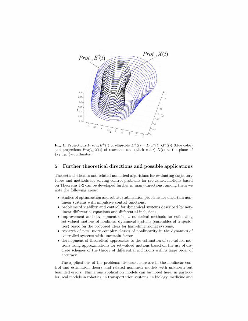
Fig. 1. Projections Proj1,2E+(t) of ellipsoids E+(t) = E(a+(t), Q+(t)) (blue color)
and projections Proj1,2X(t) of reachable sets (black color) X(t) at the plane ofx1, x2, t-coordinates.
5 Further theoretical directions and possible applications
Theoretical schemes and related numerical algorithms for evaluating trajectorytubes and methods for solving control problems for set-valued motions basedon Theorems 1-2 can be developed further in many directions, among them wenote the following areas:
• studies of optimization and robust stabilization problems for uncertain non-linear systems with impulsive control functions,• problems of viability and control for dynamical systems described by non-
linear differential equations and differential inclusions,• improvement and development of new numerical methods for estimating
set-valued motions of nonlinear dynamical systems (ensembles of trajecto-ries) based on the proposed ideas for high-dimensional systems,• research of new, more complex classes of nonlinearity in the dynamics of
controlled systems with uncertain factors,• development of theoretical approaches to the estimation of set-valued mo-
tions using approximations for set-valued motions based on the use of dis-crete schemes of the theory of differential inclusions with a large order ofaccuracy.
The applications of the problems discussed here are in the nonlinear con-trol and estimation theory and related nonlinear models with unknown butbounded errors. Numerous application models can be noted here, in particu-lar, real models in robotics, in transportation systems, in biology, medicine and
221

Fig. 2. Projection Proj1,3E+(t) of ellipsoids E+(t) = E(a+(t), Q+(t)) (blue lines)
and projections Proj1,3X(t) of reachable sets (black lines) X(t) at the plane ofx1, x3, t-coordinates.
economics. In these aspects, we would like to highlight, in particular, the stud-ies and results obtained earlier by Bayen and Rapoport[2], Cecarelli et al.[4],Koller et al.[11]), Filippova and Matviychuk[9], Kuntsevich and Volosov[13],Malyshev and Tychinskii[17], Ovsyannikov[19].
6 Conclusion
The paper deals with the state estimation problems for uncertain dynamicalcontrol systems for which we assume that the initial state is unknown butbounded with given constraints. We consider here a special case of uncertaintyand nonlinearity when the matrix parameters in state velocities are unknownbut bounded.
The system nonlinearity under study is generated also by the presence ofbilinear terms and quadratic forms in related differential equations. The prob-lem is reformulated as the control problem for the motion of related set-valuedstates.
Using the ideas developed earlier for some classes of uncertain systems wesolve here the control problem with a new class of uncertainty and with a specialstructure of nonlinearity. So we construct the external ellipsoidal estimates ofreachable sets for the system under study and find the solution of the relatedoptimization problem.
222

Fig. 3. The projections Proj2,3E+(t) of estimating ellipsoids E+(t) =
E(a+(t), Q+(t)) (indicated in blue lines) and projections Proj2,3X(t) of reachablesets (indicated in black lines) X(t) at the plane of x2, x3, t-coordinates.
Acknowledgements
The study was partially supported by the Russian Foundation for Basic Re-searches (RFBR Project No.18-01-00544).
References
1. F. Allgower and A. Zheng. (Eds.) Nonlinear Model Predictive Control, Birkhauser,Basel, 2000.
2. T. Bayen and A. Rapaport. Minimal time crisis versus minimum time to reacha viability kernel: a case study in the prey-predator model. Optimal ControlApplications and Methods, Wiley, 40(2), 330–350, 2019.
3. R. W. Brockett. On the reachable set for bilinear systems. Lecture Notes in Eco-nomics and Mathematical Systems, 111, 54–63, 1975.
4. N. Ceccarelli, M. Di Marco, A. Garulli and A. Giannitrapani. A set theoreticapproach to path planning for mobile robots. Proc. 43rd IEEE Conference onDecision and Control, Atlantis, Bahamas, Dec. 2004, 147-152, 2004.
5. F. L. Chernousko. State Estimation for Dynamic Systems, CRC Press, Boca Raton,1994.
6. F. L. Chernousko and D. Ya. Rokityanskii. Ellipsoidal bounds on reachable sets ofdynamical systems with matrices subjected to uncertain perturbations. Journalof Optimization Theory and Applications, 104, 1, 1-19, 2000.
7. T. F. Filippova. Differential equations of ellipsoidal estimates for reachable setsof a nonlinear dynamical control system. Proceedings of the Steklov Institute ofMathematics (Supplementary issues), 271, suppl.1, S75-S84, 2010.
223

Fig. 4. Reachable set X(t) and its upper ellipsoidal estimate E+(t) = E(a+(t), Q+(t))for t = 0.4 (3d-picture in the plane of state variables x1, x2, x3).
8. T. F. Filippova and D. V. Lisin. On the estimation of trajectory tubes of differentialinclusions. Proc. Steklov Inst. Math.: Problems Control Dynam. Systems. Suppl.Issue 2, S28–S37, 2000.
9. T. F. Filippova and O. G. Matviychuk. Approaches to estimating the dynamicsof interacting populations with impulse effects and uncertainty. In: C. Skiadasand Y. Dimotikalis (Eds.), 12th Chaotic Modeling and Simulation InternationalConference, CHAOS 2019, Springer Proceedings in Complexity, Springer, Cham,85–99, 2020.
10. T. F. Filippova and O. G. Matviychuk. Control problems for set-valued motionsof systems with uncertainty and nonlinearity. In: A. Tarasyev, V. Maksimovand T. Filippova (Eds.), International Conference Stability, Control, DifferentialGames, SCDG2019, September 16 20, 2019, Yekaterinburg, Russia, LectureNotes in Control and Information Sciences - Proceedings, Springer, Cham, 379–389, 2020.
11. T. Koller, F. Berkenkamp, M. Turchetta and A. Krause. Learning-basedmodel predictive control for safe exploration and reinforcement learning,arXiv:1803.08287v3 [cs.SY], https://arxiv.org/pdf/1803.08287.pdf , 1–9, 2018.
12. E. K. Kostousova. On polyhedral estimates of reachable sets of discrete-timesystems with uncertain matrices and integral bounds on additive terms. In:Y. Sergeyev and D. Kvasov (Eds.), Numerical Computations: Theory and Al-gorithms. NUMTA 2019, Lecture Notes in Computer Science, Springer, Cham,
224

11974, 124–138, 2000.13. V. M. Kuntsevich and V. V. Volosov. Ellipsoidal and interval estimation of state
vectors for families of linear and nonlinear discrete-time dynamic systems. Cy-bernetics and Systems Analysis, 51(1), 64–73, 2015.
14. A. B. Kurzhanski. Control and Observation under Conditions of Uncertainty,Nauka, Moscow, 1977.
15. A. B. Kurzhanski and I. Valyi. Ellipsoidal Calculus for Estimation and Control,Birkhauser, Boston, 1997.
16. A. B. Kurzhanski and P. Varaiya. Dynamics and Control of Trajectory Tubes.Theory and Computation, Springer-Verlag, New York, 2014.
17. V. V. Malyshev and Yu. D. Tychinskii. Construction of attainability sets andoptimization of maneuvers of an artificial earth satellite with thrusters in a stronggravitational field. Proc. of RAS, Theory and Control Systems, 4, 124-132, 2005.
18. M. Milanese, J. P. Norton, H. Piet-Lahanier and E. Walter (Eds.). BoundingApproaches to System Identification, Plenum Press, New York, 1996.
19. D. A. Ovsyannikov. Mathematical modeling and optimization of beam dynamics.IFAC Proceedings Volumes, 34(6), 13–22, 2001.
20. A. I. Panasyuk. On the equation of an integral funnel and its applications. Differ.Equations, 24(11), 1263-1271, 1988.
21. B. T. Polyak, S. A. Nazin, C. Durieu and E. Walter. Ellipsoidal parameter orstate estimation under model uncertainty. Automatica, 40, 1171-1179, 2004.
22. F. Schweppe. Uncertain Dynamic Systems, Prentice-Hall, Englewood Cliffs, NewJersey, 1973.
23. E. Walter and L. Pronzato. Identification of Parametric Models from ExperimentalData, Springer-Verlag, Heidelberg, 1997.
225

226

Interacting Populations: Dynamics andViability in Bounded Domains under
Uncertainty
Tatiana F. Filippova
Department of Optimal Control, N.N.Krasovskii Institute of Mathematics andMechanics, Ural Branch of Russian Academy of Sciences, 16 Sofya Kovalevskayastr., 620108 Ekaterinburg, Russian Federation(E-mail: [email protected])
Abstract. Nonlinear control systems which describe the dynamics of the interac-tions of predators and their preys under assumption of uncertainty in related initialconditions are studied. It is assumed that the interaction of populations occurs inlimited areas, estimated by corresponding ellipsoids. The possible presence of uncer-tainty or errors in determining the parameters of these ellipsoids and the uncertaintyin the initial conditions of the moving objects and also in some parameters of dy-namical systems are taken into account. Procedures and algorithms for evaluatingthe movements of upper estimates of reachable sets of the system under indicatedconditions of uncertainty are proposed. Numerical simulation results related to theproposed techniques and illustrating the results are also includedKeywords: Nonlinear systems, Control, Uncertainty, Ellipsoidal calculus, Viability,State estimation.
1 Introduction
In 1920 Alfred Lotka initiated the study of a predator-prey model and showedthat the populations could oscillate permanently, he further developed his re-searches in this direction and published a book (Lotka[20]). In 1926 the Italianmathematician Vito Volterra happened to become interested in the same model(Volterra[31]). Now the classical Lotka–Volterra equations have a long historyof use and researches in different branches of theory and applications, in thisfield it is worth to mention some recent approaches and results (e.g. Skiadas[29],Filippova and Matviychuk[16]) related to this class of problems.
We consider the modification of this classical problem and study it un-der conditions of uncertainty in initial system states and maybe also underuncertainty in some other parameters. We study the case when there is noprecise description of the uncertain data (noises and errors) in the model,but only some bounds on these values are specified. This situation ariseswhen we are trying to create a mathematical model that takes into accountthe absence of probabilistic data on uncertain parameters of the studied phe-nomenon, or these data are not reliable enough and therefore cannot be takeninto account. To study problems of this class, we use the set-membership es-timation approach which deals with a set of all feasible parameters vectors,consistent with the model structure, current measurements and uncertainty
227

features (Bertsekas and Rhodes[3], Kurzhanski and Valyi[18], Kurzhanski andVaraiya[19], Kurzhanski and Filippova[17], Milanese et al.[23], Schweppe[28],Walter and Pronzato[32], Chernousko[7–9], Brockett[6], Dontchev and Lem-pio[10], Veliov[30], Mazurenko[22], Polyak[26]).
In this paper we continue the study initiated in Filippova[14,15], Filippovaand Matviychuk[16] and construct the estimating procedures for reachable setsof nonlinear dynamical control systems of Lotka-Volterra type under conditionsof uncertainty and in the complicating assumption of the presence of stateconstraints on the system trajectories. It should be noted that the study ofcontrol systems with state constraints is closely related to the techniques andresults of the theory of survival, or, using the already well-established term,viability theory (Aubin and Cellina[1], Bayen and Rapaport[2], Kurzhanski andFilippova[17], Bonneuil and Mullers[5], Filippova[11]).
The viability theory presents additional convenient instruments to designand to develop mathematical and algorithmic techniques for investigating andadapting to viability constraints the complex dynamical systems under un-certainty which may be found in many domains from biology to economics,financial markets, control theory, robotics etc. Basing on above mentionedapproaches we formulate here new theoretical schemes and construct new al-gorithms for determining upper ellipsoidal estimates of reachable sets of thestudied control system with uncertainty. Numerical examples and simulationresults related to the proposed techniques and to the presented algorithms arealso included.
2 Problem formulation
2.1 Preliminary constructions
We will continue to use the notations defined earlier in Filippova and Matviy-chuk[16] but for the convenience of the reader we will nevertheless recall somebasic concepts. So Rn will be the n–dimensional Euclidean space, compRn isthe set of all compact subsets of Rn, Rn×n stands for the set of all n × n–matrices and x′y = (x, y) =
∑ni=1 xiyi be the usual inner product of x, y ∈ Rn
with prime as a transpose, the Euclidean norm is ‖x‖ = (x′x)1/2. We denoteas B(a, r) the ball in Rn, B(a, r) = x ∈ Rn : ‖x − a‖ ≤ r, I is the identityn×n-matrix, diaga1, ..., an is the diagonal n×n–matrix with elements ai atthe main diagonal and with zero entries outside it.
Denote the ellipsoid E(a,Q) = x ∈ Rn : (Q−1(x− a), (x− a)) ≤ 1 witha center a ∈ Rn and with a symmetric positive definite n × n–matrix Q. LetTr(Y ) denote the trace of n× n–matrix Y (the sum of its diagonal elements).
Consider the following system
x = Ax+ f(x)d+ u(t), x0 ∈ X0, t0 ≤ t ≤ T, (1)
where x, d ∈ Rn, ‖x‖ ≤ K (K > 0), f(x) is the nonlinear function, which isquadratic in x,
f(x) = x′Bx, (2)
228
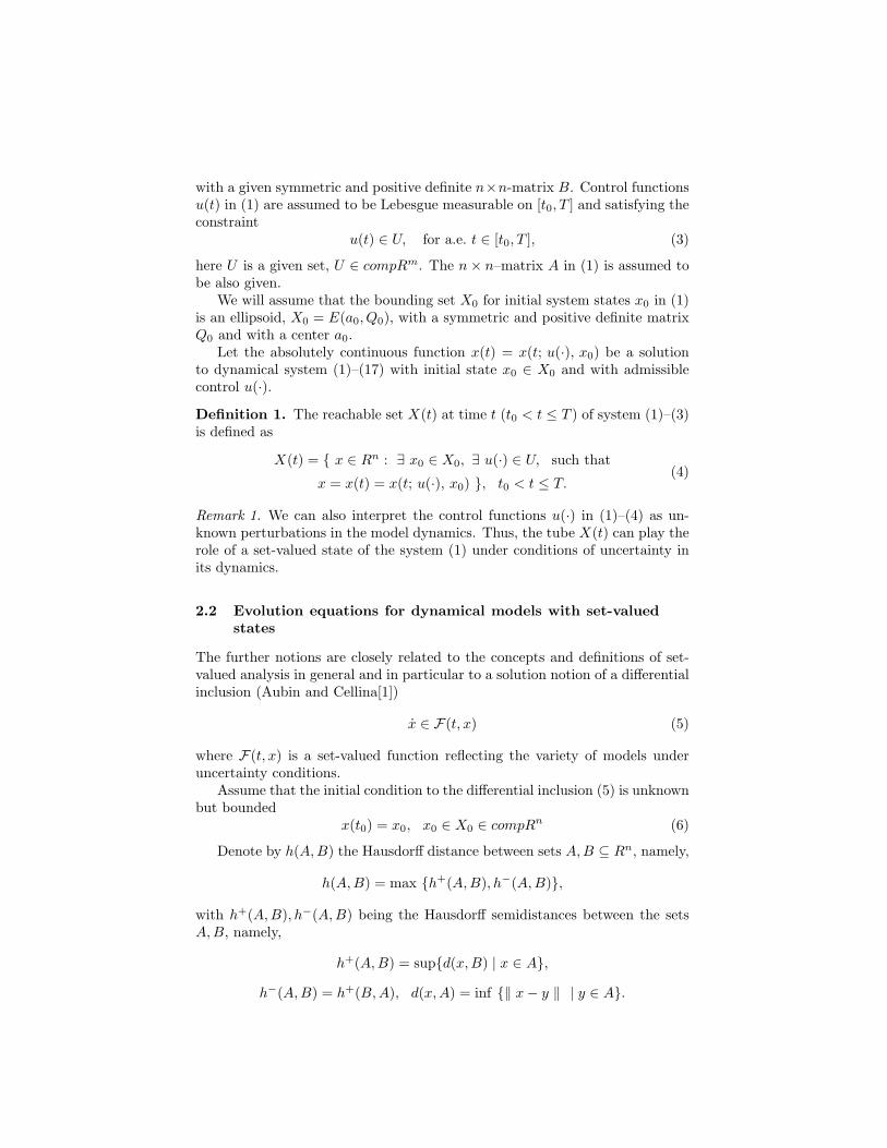
with a given symmetric and positive definite n×n-matrix B. Control functionsu(t) in (1) are assumed to be Lebesgue measurable on [t0, T ] and satisfying theconstraint
u(t) ∈ U, for a.e. t ∈ [t0, T ], (3)
here U is a given set, U ∈ compRm. The n× n–matrix A in (1) is assumed tobe also given.
We will assume that the bounding set X0 for initial system states x0 in (1)is an ellipsoid, X0 = E(a0, Q0), with a symmetric and positive definite matrixQ0 and with a center a0.
Let the absolutely continuous function x(t) = x(t; u(·), x0) be a solutionto dynamical system (1)–(17) with initial state x0 ∈ X0 and with admissiblecontrol u(·).
Definition 1. The reachable set X(t) at time t (t0 < t ≤ T ) of system (1)–(3)is defined as
X(t) = x ∈ Rn : ∃ x0 ∈ X0, ∃ u(·) ∈ U, such that
x = x(t) = x(t; u(·), x0) , t0 < t ≤ T.(4)
Remark 1. We can also interpret the control functions u(·) in (1)–(4) as un-known perturbations in the model dynamics. Thus, the tube X(t) can play therole of a set-valued state of the system (1) under conditions of uncertainty inits dynamics.
2.2 Evolution equations for dynamical models with set-valuedstates
The further notions are closely related to the concepts and definitions of set-valued analysis in general and in particular to a solution notion of a differentialinclusion (Aubin and Cellina[1])
x ∈ F(t, x) (5)
where F(t, x) is a set-valued function reflecting the variety of models underuncertainty conditions.
Assume that the initial condition to the differential inclusion (5) is unknownbut bounded
x(t0) = x0, x0 ∈ X0 ∈ compRn (6)
Denote by h(A,B) the Hausdorff distance between sets A,B ⊆ Rn, namely,
h(A,B) = max h+(A,B), h−(A,B),
with h+(A,B), h−(A,B) being the Hausdorff semidistances between the setsA,B, namely,
h+(A,B) = supd(x,B) | x ∈ A,
h−(A,B) = h+(B,A), d(x,A) = inf ‖ x− y ‖ | y ∈ A.
229

Assuming a set X0 ∈ comp Rn to be given, denote as x[t] = x(t, t0, x0) (t ∈[t0, T ]) a solution to (5) (an isolated trajectory) that starts at point x[t0] =x0 ∈ X0.
We take here the Caratheodory–type trajectory x[·], i.e. an absolutely con-tinuous function x[t] that satisfies the inclusion
d
dtx[t] = x[t] ∈ F(t, x[t]) (7)
for almost every t ∈ [t0, T ]. We assume that all the solutions x[t] = x(t, t0, x0) |x0 ∈ X0 are extendable up to T that is possible under some additional as-sumptions, Filippova[12]. Let us consider the equation
limσ→+0
σ−1h( X [t+ σ],⋃
x∈X [t]
(x+ σF(t, x)) ) = 0,
t0 ≤ t ≤ T, X [t0] = X0.(8)
Theorem 1. (Panasyuk[25], Kurzhanski and Filippova[17]) The multifunctionX [t] = X (t, t0, X0) is the unique set–valued solution to the evolution equation(8).
2.3 State constraints and viability
The main problem of the paper is to find external ellipsoidal estimates of thereachable set X(t) (t0 < t ≤ T ) and to apply these results to find the upperbounds of reachable sets for nonlinear dynamical control systems of Lotka-Volterra type considered now with the following viability (or state) constraint
x[s] ∈ Y (s), s ∈ [t0, t] (9)
where Y (t) ∈ conv Rn for t ∈ [t0, T ].This viability constraint may be induced by state restrictions defined for a
given plant model or by the so-called measurement equation
y(t) = G(t)x+ w, (10)
where y is the measurement, G(t) is a given matrix function, w is an unknownbut bounded “noise” with a given bound,
w ∈ Q∗(t), Q∗(t) ∈ comp Rp,
(here Q∗(t) is a given set-valued function).To start the analysis of the above problem consider the analogy of the funnel
equation (8) but now for the viable trajectory tubes X[t] = X(t, t0, X0):
limσ→+0
σ−1h(X[t+ σ],
⋃x∈X[t]
(x+ σF(t, x))⋂Y (t+ σ)
)= 0,
t0 ≤ t ≤ T, X[t0] = X0.
(11)
The following result is valid (under some additional assumptions on F(t, x)and Y (t)).
Theorem 2. (Kurzhanski and Filippova[17]) The set-valued function X[t] =X(t, t0, X0) is the unique solution to the evolution equation (11).
230

3 Main results
We apply here the approaches described above to study the classical modelof the Lotka-Volterra type, but now we consider these approaches with twocomplications. Namely, first, we assume that we have uncertain initial states,and second, we assume that we have an additional constraint on the currentstates of the system. In the recent paper Filippova and Matviychuk[16], weconsidered only the first problem; a more complicated case of two simultaneousconstraints is being investigated here.
3.1 Lotka-Volterra control systems under uncertainty and stateconstraints
Consider the following control system of Lotka-Volterra type which describesthe classical ecological predator-prey (or parasite-host) model with additionalcontrol functions (Bayen and Rapaport[2], Bonneuil and Mullers[5], Lotka[20],Murray[24], Prostyakov[27]):
x1(t) = ax1 − bx1x2 + u1,x2(t) = −cx2 + dx1x2 + u2,
x(t0) = x0, t0 ≤ t ≤ T. (12)
Here a, b, c, d > 0 are given and we assume that initial state vector x0 is un-known but bounded, that is we have the inclusion x0 ∈ X0, where X0 is agiven compact subset of R2. This assumption may be interpreted for examplein such a way that we do not know exactly the initial states (or amounts) ofpredators and prey. Control functions u(t) in (12) are assumed to be Lebesguemeasurable on [t0, T ], they satisfy the constraint
u(t) ∈ U, for a.e. t ∈ [t0, T ], (13)
where U is given, U ∈ compR2. The choice of control can influence, in partic-ular, the rate of change in the number of predators and prey.
Using diagonalization procedures of matrix analysis described in details inFilippova and Matviychuk[16], we transform the system (12) to the followingone (here a parameter ε > 0)
z = A∗z + f(1)ε (z) · d(1) + f
(2)ε (z) · d(2) + w(t),
z0 ∈ Z0, w ∈ W, t0 ≤ t ≤ T,(14)
where
A∗ =
(A −C−C A
),
functions f(1)ε (z) and f
(2)ε (z) are positive definite quadratic forms with matrices
B(1)ε = diag1, ε2 and B
(2)ε = diagε2, 1, respectively. The following result
may be used to produce the upper estimate of a reachable set X(t) of thesystem (12) of Lotka-Volterra type with ellipsoidal constraints on the controlfunction.
231
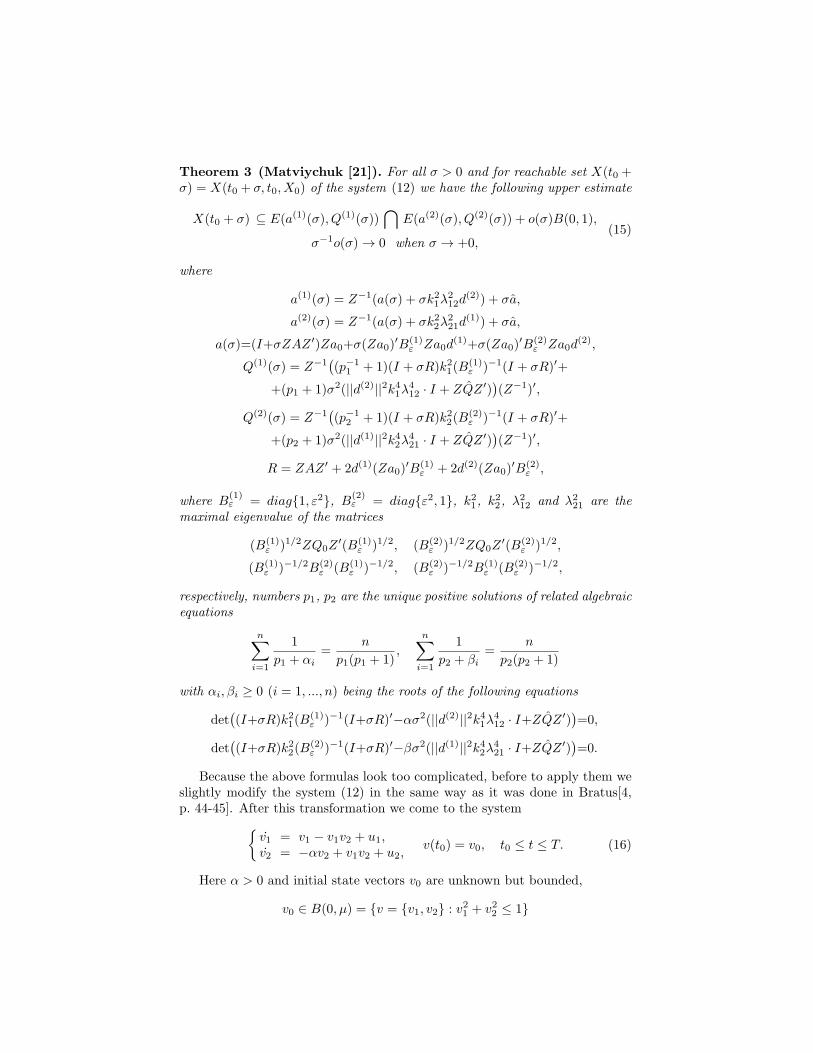
Theorem 3 (Matviychuk [21]). For all σ > 0 and for reachable set X(t0 +σ) = X(t0 + σ, t0, X0) of the system (12) we have the following upper estimate
X(t0 + σ) ⊆ E(a(1)(σ), Q(1)(σ))⋂
E(a(2)(σ), Q(2)(σ)) + o(σ)B(0, 1),
σ−1o(σ)→ 0 when σ → +0,(15)
where
a(1)(σ) = Z−1(a(σ) + σk21λ212d
(2)) + σa,
a(2)(σ) = Z−1(a(σ) + σk22λ221d
(1)) + σa,
a(σ)=(I+σZAZ ′)Za0+σ(Za0)′B(1)ε Za0d
(1)+σ(Za0)′B(2)ε Za0d
(2),
Q(1)(σ) = Z−1((p−11 + 1)(I + σR)k21(B(1)
ε )−1(I + σR)′+
+(p1 + 1)σ2(||d(2)||2k41λ412 · I + ZQZ ′))(Z−1)′,
Q(2)(σ) = Z−1((p−12 + 1)(I + σR)k22(B(2)
ε )−1(I + σR)′+
+(p2 + 1)σ2(||d(1)||2k42λ421 · I + ZQZ ′))(Z−1)′,
R = ZAZ ′ + 2d(1)(Za0)′B(1)ε + 2d(2)(Za0)′B(2)
ε ,
where B(1)ε = diag1, ε2, B(2)
ε = diagε2, 1, k21, k22, λ212 and λ221 are themaximal eigenvalue of the matrices
(B(1)ε )1/2ZQ0Z
′(B(1)ε )1/2, (B(2)
ε )1/2ZQ0Z′(B(2)
ε )1/2,
(B(1)ε )−1/2B(2)
ε (B(1)ε )−1/2, (B(2)
ε )−1/2B(1)ε (B(2)
ε )−1/2,
respectively, numbers p1, p2 are the unique positive solutions of related algebraicequations
n∑i=1
1
p1 + αi=
n
p1(p1 + 1),
n∑i=1
1
p2 + βi=
n
p2(p2 + 1)
with αi, βi ≥ 0 (i = 1, ..., n) being the roots of the following equations
det((I+σR)k21(B(1)
ε )−1(I+σR)′−ασ2(||d(2)||2k41λ412 · I+ZQZ ′))=0,
det((I+σR)k22(B(2)
ε )−1(I+σR)′−βσ2(||d(1)||2k42λ421 · I+ZQZ ′))=0.
Because the above formulas look too complicated, before to apply them weslightly modify the system (12) in the same way as it was done in Bratus[4,p. 44-45]. After this transformation we come to the system
v1 = v1 − v1v2 + u1,v2 = −αv2 + v1v2 + u2,
v(t0) = v0, t0 ≤ t ≤ T. (16)
Here α > 0 and initial state vectors v0 are unknown but bounded,
v0 ∈ B(0, µ) = v = v1, v2 : v21 + v22 ≤ 1
232

and control functions u(t) satisfy the following constraint (with r > 0)
u(t) ∈ B(0, r), for a.e. t ∈ [t0, T ]. (17)
Replace here ones again the variables as w1 = v1+v2, w2 = v1−v2 and considerthe system
w = Dw + d(1)f1(w) + d(2)f2(w),
w(t0) = w0 ∈ B(0, r), r = 2−1/2, t0 ≤ t ≤ T,(18)
with f1(w) = 2w21 + w2
2, f2(w) = w21 + 2w2
2,
D =
(1−α2
1+α2
1+α2
1−α2
)(19)
and with related trajectory tube denoted as W (·) = W (·, t0, X0).
Theorem 4. For all σ > 0 and for W (t0+σ) = W (t0+σ, t0, X0) the followingupper estimate is true
W (t0 + σ) ⊆ E(a(1)(σ), Q(1)(σ))⋂
E(a(2)(σ), Q(2)(σ)) + o(σ)B(0, 1), (20)
where σ−1o(σ) → 0 when σ → +0 and parameters of the estimating ellipsoidsE(a(1)(σ), Q(1)(σ)) and E(a(2)(σ), Q(2)(σ)) are defined in Theorem 3 with thefollowing simplifications
k21 = k22 = 2/r2, λ212 = λ221 = 2, a = a = 0,
d(1) = −d(2) = −(0, 1)′, Q = r2I,
B(1) =
(2 0
0 1
), B(2) =
(1 0
0 2
).
Proof. The proof of the above upper estimates follows the scheme used inFilippova and Matviychuk[16].
3.2 Iterative algorithm and numerical simulation
The following iterative algorithm may produce the external ellipsoidal tubefor the reachable set X(t), t ∈ [t0, T ] in numerical modelling. Note that, incomparison with the algorithm given in Filippova and Matviychuk[16], it issomewhat more complicated in calculations, since additional steps appearedhere.
Algorithm. Subdivide the time segment [t0, T ] into subsegments [ti, ti+1]where ti = t0 + ih (i = 1, . . . ,m), σ = (T − t0)/m, tm = T .
• Given X0 = E(a0, Q0), find ellipsoids E(a(1)(σ), Q(1)(σ)) andE(a(2)(σ), Q(2)(σ)) from Theorems 3–4.
233
• Find the smallest (with respect to some criterion [18,7]) ellipsoid E(a1, Q1)which contains the intersection
E(a(1)(σ), Q(1)(σ))⋂E(a(2)(σ), Q(2)(σ)) ⊆ E(a1, Q1).
• Find the new ellipsoid E(a2, Q2) such that we have
E(a1, Q1)⋂Y ⊆ E(a2, Q2)
(this is a correction taking into account state constraints)• Consider the system on the next subsegment [t1, t2] with E(a2, Q2) as the
initial ellipsoid at the next instant t1.• Further steps repeat above iterations. At the end of the process we will
get the external estimate E(a+(t), Q+(t)) of the tube X(t) with accuracytending to zero when m→∞.
Example 1. Consider the following control system of Lotka–Volterra type:x1(t) = x1 − x1x2 + u1,x2(t) = −x2 + x1x2 + u2,
x0 ∈ X0, t0 ≤ t ≤ T.(21)
Here we take t0 = 0, T = 1, X0 = B(0, 1) and U = B(0, 0.1). We assume alsothat we have the following additional state constraint
x[s] ∈ E(d,D), s ∈ [t0, t]
with d = (0.1, 0) and
D =
(2.25 0
0 0.56
).
The trajectory tube X(t) and some reachable sets are shown in the Fig. 1and Fig. 2. Ellipsoidal estimates for the reachable set X(0.01) which werefound on the basis of results of Theorems 3,4 are shown in Fig. 2. Several stepsof the main Algorithm of external ellipsoidal estimating the reachable set X(t)with the resulting ellipsoidal tube E(a+(t), Q+(t)) are shown in the Fig. 2.
4 Conclusions
We considered the problems of state estimation for dynamical control systemswith unknown but bounded initial state. The solution was studied through thetechniques of trajectory tubes of related differential inclusions.
The problem of estimating reachable sets of nonlinear dynamical controlsystems of Lotka-Volterra type which describe the dynamics of the interactionof predators and their preys under uncertainty conditions and state constraintswas studied. Applying results of the theory of trajectory tubes of controlsystems we found upper ellipsoidal estimates of related reachable sets.
The algorithms of constructing ellipsoidal estimates are given, numericalsimulation results related to the proposed techniques and illustrating the algo-rithms are included.
234

Fig. 1. Estimates of X(t) of the system (21).
Fig. 2. Steps of the Algorithm of ellipsoidal estimating process for the trajectorytube X(t) (σ = 0.01).
Acknowledgements
The research was supported by the Research and Education Center of KrasovskiiInstitute of Mathematics and Mechanics (Ural Branch of Russian Academy ofSciences, Ekaterinburg, Russia) in the framework of the Ural MathematicalCenter (Project “Set-Valued Dynamics in Control and Estimation Problemsfor Dynamical Systems with Uncertainty”).
235

References
1. J.-P. Aubin and A. Cellina. Differential Inclusions: Set-Valued Maps and ViabilityTheory. Springer-Verlag, Berlin, 1984.
2. T. Bayen and A. Rapaport. Minimal time crisis versus minimum time to reacha viability kernel: a case study in the prey-predator model. Optimal ControlApplications and Methods, Wiley, 40(2), 330–350, 2019.
3. D. P. Bertsekas and I. B. Rhodes. Recursive state estimation for a set-membershipdescription of uncertainty. IEEE Transactions on Automatic Control, 16, 117–128, 1971.
4. A. S. Bratus, A. S. Novozhilov and A. P. Platonov. Dynamical Systems and Modelsof Biology. Fizmatlit, Moscow, 2010.
5. N. Bonneuil and K. Mullers. Viable populations in a prey-predator system.Journalof Mathematical Biology, 35, 261–293, 1997.
6. R. W. Brockett. On the reachable set for bilinear systems. Lecture Notes in Eco-nomics and Mathematical Systems, 111, 54–63, 1975.
7. F. L. Chernousko. State Estimation for Dynamic Systems. CRC Press, Boca Raton,1994.
8. F. L. Chernousko. Ellipsoidal approximation of the reachable sets of linear systemswith an indeterminate matrix. Applied Mathematics and Mechanics, 60, 6, 940–950, 1996.
9. F. L. Chernousko and D. Ya. Rokityanskii. Ellipsoidal bounds on reachable sets ofdynamical systems with matrices subjected to uncertain perturbations. Journ.of Optimiz. Theory and Appl., 104, 1, 1-19, 2000.
10. A. L. Dontchev and F. Lempio. Difference methods for differential inclusions: asurvey. SIAM Review, 34, 263–294, 1992.
11. T. F. Filippova. A note on the evolution property of the assembly of viable so-lutions to a differential inclusion. Computers & Mathematics with Applications,25, 2, 115–121, 1993.
12. T. F. Filippova. Trajectory tubes of nonlinear differential inclusions and stateestimation problems. J. of Concrete and Applicable Mathematics, Eudoxus Press,LLC, 8, 454–469, 2010.
13. T. F. Filippova. Set-valued dynamics in problems of mathematical theory of con-trol processes. International Journal of Modern Physics, Series B (IJMPB), 26,25, 1–8, 2012.
14. T. F. Filippova. Differential equations of ellipsoidal state estimates for bilinear-quadratic control systems under uncertainty. J. Chaotic Modeling and Simulation(CMSIM), 1, 85–93, 2017.
15. T. F. Filippova. External estimates for reachable sets of a control system withuncertainty and combined nonlinearity. Proc. Steklov Inst. Math., 301, suppl.1,32–43, 2018.
16. T. F. Filippova and O. G. Matviychuk. Approaches to estimating the dynamics ofinteracting populations with impulse effects and uncertainty, Springer Proceed-ings in Complexity, C. Skiadas, Y. Dimotikalis (Eds.), 85–99, Cham, Springer,2020.
17. A. B. Kurzhanski and T. F. Filippova. On the theory of trajectory tubes a math-ematical formalism for uncertain dynamics, viability and control. In: Advancesin Nonlinear Dynamics and Control: a Report from Russia, Progress in Systemsand Control Theory, A. B. Kurzhanski (Ed.), 17, 22–188. Birkhauser, Boston,1993.
18. A. B. Kurzhanski and I. Valyi. Ellipsoidal Calculus for Estimation and Control.Birkhauser, Boston, 1997.
236

19. A. B. Kurzhanski and P. Varaiya. Dynamics and Control of Trajectory Tubes.Theory and Computation. Springer-Verlag, New York, 2014.
20. A. J. Lotka. Elements of Physical Biology. Williams and Wilkins, Baltimore. 1925.21. O. G. Matviychuk. Estimates of the reachable set of nonlinear control system
under uncertainty. AIP Conf. Proc., 2025, 100005, 1–9, 2018.22. S. S. Mazurenko. A differential equation for the gauge function of the star-shaped
attainability set of a differential inclusion. Doklady Mathematics, 86, 1, 476–479,2012.
23. M. Milanese, J. P. Norton, H. Piet-Lahanier and E. Walter (Eds.). BoundingApproaches to System Identification. Plenum Press, New York, 1996.
24. J. D. Murray. Mathematical Biology. Springer, New York, 1993.25. A. I. Panasyuk. Equations of attainable set dynamics, Part 1: Integral funnel
equations. J. Optimiz. Theory Appl., 2, 349–366, 1990.26. B. T. Polyak, S. A. Nazin S.A., C. Durieu and E. Walter. Ellipsoidal parameter
or state estimation under model uncertainty. Automatica, 40, 1171–1179, 2004.27. P. Prostyakov. Construction of the reachability set of the Lotka-Volterra system.
Differ. Equ., 42, 3, 391–399, 2006.28. F. Schweppe. Uncertain Dynamic Systems. Prentice-Hall, Englewood Cliffs, New
Jersey, 1973.29. C. H. Skiadas, A Two Population Model for the Stock Market Problem, Chaotic
Systems: Theory and Applications, C. H. Skiadas and I. Dimotikalis, Eds, WorldScientific, 2010, 302–308.
30. V. M. Veliov. Second order discrete approximations to strongly convex differentialinclusion. Systems and Control Letters, 13, 263–269, 1989.
31. V. Volterra. Variazioni e fluttuazioni del numero dindividui in specie animali con-viventi. Memoria della Reale Accademia Nazionale dei Lincei, Ser. VI, Vol. 2,31–113, 1926.
32. E. Walter and L. Pronzato. Identification of Parametric Models from ExperimentalData. Springer-Verlag, Heidelberg, 1997.
237

238

Battle of Salamis: Greeks were destined to win
Konstantina Founta1, Loukas Zachilas2
1 Department of Economics, University of Thessaly, Volos, Greece
(E-mail: [email protected]) 2
Department of Economics, University of Thessaly, Volos, Greece
(E-mail: [email protected])
Abstract. In this paper we present a new non–linear, discrete, dynamical system trying to
model the historic battle of Salamis (480 BC) between Greeks and Persians. The model
describes the most effective strategic behavior between two participants during a battle or
in a war. Moreover, we compare the results of the dynamical analysis to Game Theory,
considering this conflict as a dynamic game.
Keywords: Battle of Salamis, Discrete Systems, Modeling Strategic Behavior, Game
Theory.
1 Introduction
The model approaches short–term conflicts between two participants (players),
where one is weaker than the other opponent. Also, the parameters (that we use
in Eq. 1, see below) are the most crucial factors in order to highlight the optimal
way to achieve a decisive victory.
The solution of the equations of the dynamical system (called equilibrium point)
shows what kind of behavior each player should adopt, i.e. an aggressive or
defensive one. In this way, according to Game Theory, the optimum strategic
behavior is called Nash Equilibrium [9].
One of the most representative games of Evolutionary Game Theory is the so-
called game “Hawk – Dove”, which was originally developed by Smith and Price
[10] to describe animal conflicts and is quite similar to our attempt. We will
present below the game and its results.
The game “Hawk – Dove” has many applications in everyday life. There are two
animals (or two players) fighting for the same resource. Each of them can behave
either as a hawk (i.e. fight for the resource) or as a dove (i.e. abandon the resource
before the conflict escalates into a fight). Individuals have a benefit B if they win
and a cost C if lose.
If a Hawk meets a Hawk, they will fight and one of them will win the resource;
average payoff is (B-C)/2. If a Hawk meets a Dove, the Dove immediately
withdraws, so the payoff of the Dove is zero, while the payoff of the Hawk is B.
If a Dove meets a Dove, the one who first gets hold of the resource keeps it, while
the other does not fight for it; average payoff B/2. The strategic form of the game
is given by the payoff matrix:
𝑃𝑎𝑦𝑜𝑓𝑓𝐻,𝐷 = ((𝐵 − 𝐶)/2 𝐵
0 𝐵/2)
239

2 Solution of the game “Hawk – Dove” We set the benefit B = 2 if a player wins, and the cost C = 1 if a player loses.
Using the Gambit1 software (16.0.1), we find Nash equilibriums and the dominant
strategy.
Fig. 1: The results of "Hawk - Dove" game.
Fig. 1 shows us the payoff matrix and the two Nash equilibriums. If both players
behave as a Hawk, the one who first injures the other wins. We set the player 1
starts and injures the player 2, thus player 1 wins. If someone behaves as a Hawk
and the other behaves as a Dove, then the player with the aggressive behavior
(Hawk) wins and takes all the resource. If both players behave as a Dove, then
they share the resource.
Regarding Nash equilibriums, there are two pure strategies. On the one hand, both
players behave as Hawks and on the other hand, player 1 behaves as a Hawk and
player 2 as a Dove. Moreover, we can observe that player 1 behaves as a Hawk
in both cases and player 2 behaves either as a Hawk or as a Dove, but in each case
player 1 wins.
We should note that if player 2 injures first player 1, the Nash equilibriums would
be different.
1 McKelvey, Richard D., McLennan, Andrew M., and Turocy, T. L., 2014.
240

Fig. 2: Dominant Strategy.
Fig. 2 shows the dominant strategy of the game, where player 1 behaves as a
Hawk independently of the player’s 2 behavior (i.e. Hawk or Dove). Therefore,
the first dominant strategy may not be effective, because both players behave as
Hawks and player 1 wins the half of the resource and does not maximize his profit.
Although, if the player behaves as a Hawk, knowing that the other player behaves
as a Dove, then he takes all the resource (maximum profit). Thus, we believe that
the second Nash equilibrium is more effective and optimum strategy.
3 The Dynamical Model It is widely acknowledged that the military strategy is the combination of ends,
ways and means [7]. In our attempt to study the strategic behavior of two warring
parties, we developed a new non-linear discrete system of two equations based on
the above phrase. The main objective of the model is to simulate the way by which
the two opponents behave strategically, where the one is weaker than the other.
At the same time, in Game Theory, the war is considered as a dynamic game
where the strategies of the players are studied by calculating their optimal strategy
(Nash equilibrium). In this research, we tried to compare the results of the Game
Theory with those from the analysis of the discrete dynamical system. At the end
of the analysis, the optimum and effective strategy for both participants (players)
will be suggested.
The model, which is applied in short-term conflicts and describes the strategic
behavior of each participant, is given by Eq. 1:
𝑥𝑡+1 = 𝑃𝑥 + 𝑇𝑁𝑥 − 𝐺 ∙ (𝐷𝑦 + 𝐸𝑥) ∙ 4𝑦𝑡 ∙ (1 − 𝑦𝑡)
𝑦𝑡+1 = 𝑃𝑦 + 𝑇𝑁𝑦 − (1 − 𝐺) ∙ (𝐷𝑥 + 𝐸𝑦) ∙ 4𝑥𝑡 ∙ (1 − 𝑥𝑡) [1]
where:
𝑥𝑡: The strategic behavior of any form of social organization x (state, country,
etc.) at the time t.
241

𝑦𝑡: The strategic behavior of any form of social organization y (state, country,
etc.) at the time t.
𝑥𝑡+1: The optimal strategic behavior of any form of social organization x at the
(next moment of) time t + 1.
𝑦𝑡+1: The optimal strategic behavior of any form of social organization y at the
(next moment of) time t + 1.
We consider 𝑥𝑡 , 𝑦𝑡 , 𝑥𝑡+1, 𝑦𝑡+1 ∈ [0,1], because the logistic equation is defined in
[0,1], which is derived from the study of biological populations reproduced in
discrete time [6]. It’s the evolution of the population model of Malthus [8] and
shows that the exponential growth cannot tend to infinity, but there is a critical
point, i.e. a saturation. In other words, it is not possible for someone to win and
the other to lose continuously. Also, each optimal strategic behavior, at the time
t, affects the next move – strategic behavior, at the time t + 1, of the opponent.
In addition, we can interpret the values of variables (and parameters, as shown
below) as percentages or probabilities, which help us to explain the results; these
are also explained through the Game Theory.
Moreover, if the value of 𝑥𝑡+1 (or 𝑦𝑡+1, respectively) equals to 0, it indicates the
fully defensive strategic behavior of participant x (or y respectively), while if it
equals to 1, then it indicates the fully aggressive behavior of participant x (or y
respectively).
The parameters of Eq. 1 are the main and most important factors that could affect
the strategic behavior of x (or y, respectively). In particular:
The parameter 𝑷𝒙 represents the strength (economic, military, population,
territorial) of x and 𝑷𝒚 is the strength of y, respectively. These two parameters
indicate the substance of each form of social organization compared to the other.
𝑻𝑵𝒙 and 𝑻𝑵𝒚 represents the Technological Naval capability and evolution of x
and y, respectively. These two parameters are also defined in comparison with the
technological capability and evolution of the other participant and describe the
means mentioned by [7].
The parameter G represents the geographical location (geophysical terrain) of the
area where the battle or the war is taking place. We believe that this is another
part of the military strategy, namely the ways [7]. Trying to emphasize the
importance of this parameter and how it can be an advantage or disadvantage for
each participant, we set in the first equation as G and in the second equation as 1
– G. The closer to the 1 the value of the parameter, the easier the geophysical
terrain of the area is.
The parameter 𝑫𝒙 represents the damages caused by x to y and respectively,
𝑫𝒚 represents the damages that y brings to x. The damages which we refer to may
be economic, territorial, military, etc. or even deception and damaging of the
psychological part of the opponent. Moreover, these two parameters complete the
last part of the military strategy, namely the ends [7].
The parameter 𝑬𝒙 represents the expenses of participant x and 𝑬𝒚 the expenses of
participant y, respectively. In other words, these denote the preparation costs of
each participant for a battle (or war), compared to each other.
242

All the parameters that have been presented above should belong to [0,1].
Namely, 𝑃𝑥 , 𝑃𝑦 , 𝑇𝑁𝑥 , 𝑇𝑁𝑦 , 𝐺, 𝐷𝑥 , 𝐷𝑦 , 𝐸𝑥 , 𝐸𝑦 ∈ [0,1].
In the next section, we present the dynamic analysis and the results from the
application of Eq. 1 in naval battle of Salamis.
4 The case of (naval) Battle of Salamis
The naval battle of Salamis was an important battle of the second Persian invasion
in Greece and has been estimated to being held on September 28th, 480 BC in the
Salamis straits (in the Saronic Gulf near Athens). The two warring parties were
the Greeks (Hellenic alliance) and the Persian Empire [2].
After the fall of Thermopylae, the Persians proceeded to Athens. The Greeks had
been advised by the Oracle of Delphi, that only the "wooden walls" would save
them and they considered that this referred to a fight in the sea [5].
A few days before the battle, the meeting of the Greek admirals had to decide the
geographic location of the battle. On the one hand, the Spartan General Evriviades
proposed to fight in the Isthmus of Corinth, under the main argument that in case
of failure it would be possible for them to continue to fight into the center of the
Peloponnese. On the other hand, the Athenian General Themistocles insisted to
fight in Salamis straits. He believed that if he forced the Persians to attack there,
the numerous Persian ships couldn’t extent highlighting their dominance.
Ultimately, the council considered that Themistocles’ argument was better and
decided to support it [1].
The Greek fleet was estimated by Herodotus in 380 triremes and Aeschylus gave
a round 300 triremes, but we can’t be certain for the exact number. On contrary,
the Persian fleet was estimated in 500-600 triremes2. Herodotus describes the
Persian ships as “better sailing”, when compared to the Greek fleet. This may be
attributable to a combination of factors such as lightness of materials and structure
of the ship, better seamanship and more extensive naval experience. The triremes
of Hellenic alliance were heavier and more durable. However, Herodotus reports
that these ships were equipped with an embolism, with which they sank the enemy
ships. They used two attacking maneuvers: diekplous, (i.e. attack from the rear or
sides with a sharp turn) and periplous, (flanking or enveloping move, which
generally gave an extra benefit against superior numbers in open water). The
purpose of both was to ram the enemy in the side. In this way, they achieved
serious damages or even the complete destruction of the Persians ships. On the
contrary, the Persian tactic was “ramming and boarding” [11].
2 Aeschylus, writing decades earlier, also gives 1,207 triremes, but Herodotus writes,
shortly before battle took place, that the Persian fleet wasn’t much bigger than Greek.
Because of a weather phenomenon (storms) 600 ships sank (400 at the coast of Magnesia,
north of Artemisium and 200 in Euboea).
243

Fig. 3: The battle of Salamis.
Source: Burn, A. R. (1962). Persia and the Greeks, New York: Minerva Press
At dawn (if the date of the battle was indeed 28th Sept.), the two fleets were ready
for the naval conflict. Xerxes, sure of his victory, sat on a throne on mountain
Aigaleo, to enjoy the war spectacle. The narrowness of the space and the limited
extent of the sea did not allow the Persians to use the major of their force in the
front line. Thus, the number of ships was approximately equal. In this naval
battle, the bravery and dexterity of the Greek fleet played an important role. They
fought aggressively to defend their moral values and their freedom [1].
Herodotus reports that “the Greeks fought with discipline and held their
formation, but the Persians did not seem to be following any plan, so things were
bound to turn out for them as they did”. Also, Aeschylus mentions that
Themistocles must be given the credit for their battle and the winning tactics. The
turning point of the battle came as the Persians “suffered their greatest losses
when the ships in their front line were put to fight and those following, pressing
forward to impress the King (i.e. Xerxes) with their deeds, became entangled with
them as they tried to escape”, as Herodotus comments [11].
The naval battle evolved rapidly and by the noon it was visible that the Greeks
would win. The Persian fleet had crushed, while the Greek fleet continued to
haunt them, killing the helpless, non–swimming soldiers. This brought the battle
to an end, leaving the Greek force in full control of the straits [1].
When the battle was over, a Roman source mentions that Greeks lost more than
40 triremes and Persians more than 200 ones [11]. The victory of the Greek force
was of major importance, since they managed to cause the collapse of the Persian
morale, which is evidenced by the abandonment of the battle. In addition, the right
244

decision of Themistocles for the geographic location of the naval battle was one
of the most intelligent movements to bring the Greek victory.
5 Applying the model in naval battle of Salamis – Approaching
the reality
Starting the dynamical analysis of the naval battle of Salamis, we set the initial
conditions in Eq. 1, which represent as much as possible the historical events of
the battle. Specifically:
(a) We set Greeks as the weak participant – player (x) and Persians as the
powerful participant – player (y).
(b) The strength of Hellenic alliance, 𝑃𝑥 = 0.25 and the strength of Persian
empire, 𝑃𝑦 = 0.8.
(c) The technological naval capability of Greeks, 𝑇𝑁𝑥 = 0.7 and the
technological naval capability of Persians, 𝑇𝑁𝑦 = 0.35.
(d) The geographic location of the naval battle, G = 0.4, i.e. the Salamis
straits, which are an advantage point for the Greek fleet.
(e) The damage caused to Persian side was huge, so we set 𝐷𝑥 = 0.8 and 𝐷𝑦 = 0.2.
(f) The preparation costs of this battle for each participant: 𝐸𝑥 = 0.3, 𝐸𝑦 =
0.7, respectively. According to Kyriazis and Zouboulakis [5], 100 new
Athenian triremes were built under the Athenian Naval Law of
Themistocles. Each one cost one talent (6000 ancient drachmae), so the
total cost was 100 talents (or 600.000 ancient drachmae). In 480 BC, the
Athenian fleet was comprised of 200 triremes, equivalent to the two
thirds of the total Greek strength. However, the Persian ships were
similar in shape, so we assume that the cost of each ship was similar.
Thus, it is obvious that the Persians spent more money to support their
expedition to the Greek territories than the Greeks.
With these initial conditions, we solve the system (Eq.1), by using the
mathematical software Maxima3 (5.39.0), calculating the equilibrium points.
Then, we study more extensively the behavior of the model and we present
bifurcation diagrams and timeseries diagrams using the software E&F Chaos4.
Solving the system (Eq.1), there are two equilibrium points: E1 (x* = 0.75, y* =
0.475) and E2 (x** = 0.96, y** = 1.012). According to Game Theory, these two
fixed points are considered as Nash Equilibriums [9]. Below, the stability of the
fixed points will be examined.
The Jacobian matrix is:
𝐽 = (0 0.8𝑦 − 0.8(1 − 𝑦)
3.6𝑥 − 3.6(1 − 𝑥) 0)
3 https://sourceforge.net/projects/maxima/files/Maxima-Windows/5.39.0-Windows/ 4 E & F Chaos: written by Diks, C., Hommes, C., Panchenko, V., van der Weide, R.,
(2008).
245

We calculate the Jacobian matrix at the equilibrium point E1:
𝐽∗ = (0 0.038
1.803 0)
The determinant of J* is det (J*) = 0.069 > 0.
The trace of J* is trace(J*) = 0.
The eigenvalues of J* is (0.264i, -0.264 i); two complex roots.
The discriminant 𝛥 = 𝑡𝑟𝑎𝑐𝑒(𝐽∗)2 − 4 ∙ 𝑑𝑒𝑡(𝐽∗)= 0.2788 < 0.
Therefore, the equilibrium point E1 is a stable – center.
Studying the second fixed point E2, the Jacobian matrix at the equilibrium point
is:
𝐽∗∗ = (0 0.82
3.314 0)
The determinant of J** is det (J**) = 2.718 < 0.
The trace of J** is trace(J**) = 0.
The eigenvalues of J** is (1.648, 1.6487); two real roots.
The discriminant is 𝛥 = 𝑡𝑟𝑎𝑐𝑒(𝐽∗∗)2 − 4 ∙ 𝑑𝑒𝑡(𝐽∗∗) 10.874 > 0.
Therefore, the equilibrium point E2 is a saddle point.
Consequently, we accept the fixed point E1 (x* = 0.75, y* = 0.475) and reject E2
(x** = 0.96, y** = 1.012), because the value of y** is greater than 1.
Thus, we continue the analysis for the fixed point E1. Interpreting this equilibrium
point, we confirm the aggressive (strategic) behavior of Greeks; since the value
of x* is close to 1 and the mild (strategic) behavior of Persians; since they thought
it would be an “easy win”.
Indeed (historically), the courage of the Greeks, their technological naval skills,
and the advantageous geographical location contributed in this aggressive
behavior. As far as the Persians are concerned, their mild (strategic) behavior is
due to the fact that they underestimated their enemy, since they regarded that the
Greeks are an easy target, and they would achieve a decisive victory.
Connecting the game “Hawk – Dove” to the naval battle of Salamis, player 1 (red)
is “Persians” and player 2 (blue) is “Greeks” (Fig. 4). The Hellenic alliance had
an aggressive behavior (Hawk) and the Persians behaved as a Dove. According
the Nash equilibriums that have been mentioned above (See 2), the Greeks (player
2) should behave as a Hawk (i.e. aggressive), regardless of Persian’s behavior, so
as to win this battle.
246

Fig. 4: Time series diagram - x (Greeks; blue) and y (Persians; red).
Fig. 4 shows us how the two warring parties behave (strategically). In particular,
it represents the optimal strategic behavior of Greeks and Persians in Salamis
straits for a time interval of 24 hours. We can observe an oscillation, at the
beginning, until t = 6 h. (both lines) and then it is normalized and balanced. That
means that the duration of the main battle was approximately 6 hours. Indeed,
according to historical documents, the battle started at dawn (approximately at
06:00 am) and the Greek victory was visible at noon.
Fig. 5: Bifurcation Diagram for different values of G.
x (Greeks; blue) and y (Persians; red).
Fig. 5 presents the strategic behavior of Greeks (blue) and Persians (red) as the
parameter G changes. We observe for the positive values of G, the blue line is
247

above the red until G = 0.64 (critical value) and for G > 0.64 the red line is above
the blue. The increase of the value of parameter signifies the change of the
geographical location (a more open sea), which becomes more difficult for Greeks
and in contrary easier for Persian. Thus, we approve that if the location of the
naval battle was in an open sea, the Persians would have a crucial advantage,
which would possibly lead to win this conflict.
Although we did not study the negative values of parameter G, we believe that
there are some unpredictable geophysical factors (e.g. meteorological phenomena
to influence the outcome of the conflict), which are surprisingly interesting.
Specifically, we refer to weather conditions, such as air, ripple, etc., which can
affect the geophysical terrain of the area. Due to these weather phenomena, period
doubling bifurcations and chaos appear and we cannot predict what could happen
in the battle for these values of G.
Fig. 6: Bifurcation diagrams for different values of parameters 𝑇𝑁𝑥 and 𝑇𝑁𝑦 .
Fig. 6a: x (Greeks; blue) and Fig. 6b: y (Persians; red).
Fig. 6 depicts the technological evolution and capability of x (Greeks; blue) and
y (Persians; red), respectively. In the left diagram (Fig. 6a), for the negative values
of parameter 𝑇𝑁𝑥, we can distinguish a pair of bubble bifurcations, while
afterwards we have the well-known period-doubling scenario to chaos. A possible
interpretation of this chaotic scenario is the uncertainty of Greeks in technological
capability – first attempts to construct ships. The first ships, as Krasanakis [4]
mentions, were floating planks and carved tree trucks only with oars. Since the
ships were primitive, the situation was unstable (there is chaos in this range of
values) because they were not capable to fight in naval battles. Later, the sails
were invented, which gave high speed to ships, and they were consisted no more
than wood but iron. For this reason, we have bubble bifurcations, which indicate
the technological alternatives that existed for the construction of the ships. In the
interval of positive values of 𝑇𝑁𝑥, there is stability with two fixed points. Here,
it’s the beginning of better shipbuilding ability and new expertise ship
construction. Finally, there is one equilibrium point which shows the better
version of ships, of that period, namely Triremes. Triremes were wooden
248

warships which move either with sails or oars. Moreover, in the positive values
of the parameter 𝑇𝑁𝑥, the increasing of the slope of the curve is visible, which,
on the one hand, it means that in 480 BC the triremes were an innovation in
shipbuilding and on the other hand, it shows the excellent naval capability of the
Greeks.
Persians, through the years, developed technological equipment because of their
expansive mania to conquer Greece. Comparing the Figures 6a and 6b, it seems
that Persians had a lower technological development than Greeks, since they
focused more on land army than on warships. Their ships were mainly used
as troopships rather than battleships [11].
Conclusions In this article, a new non – linear discrete model has been presented, which
simulates the optimum strategic behavior of two warring parties for short–term
battles. In addition, we try to compare this model with the game “Hawk – Dove”,
applying this attempt in the naval battle of Salamis. Based on the results we have
extracted, we (mathematically) proved the historical events of this conflict.
Specifically, the Greek’s strategic behavior fits with the aggressive behavior of
the Hawk and as well as the Persian’s strategic behavior fits with the more
defensive behavior of the Dove in the game. Moreover, the estimated duration of
the battle was proved as well as the dominance of the Greek fleet in the Salamis
straits. Finally, the technological naval capability of the Greek alliance was able
to cause serious damages to the opponent and led them to a crashing defeat.
References
1. Burn, A. R. Persia and the Greeks, New York: Minerva Press, 1962.
2. Goodwin, W. The battle of Salamis. Harvard Studies in Classical Philology, Vol. 17,
pp. 74-101, 1906.
3. Green. P. The Greco – Persian Wars, University of California Press, 1998.
4. Krasanakis, A. Naval History of the Greek Nation. Athens Press, 2008.
ISBN: 9789604841592.
5. Kyriazis, N., Zouboulakis, M. Democracy, Sea Power and Institutional Change: An
Economic Analysis of the Athenian Naval Law. European Journal of Law and
Economics, 17: 117–132, Kluwer Academic Publishers, 2004.
6. Lorenz, E. “The problem of deducing the climate from the governing equations”,
Tellus 16, 1964.
7. Lykke, A. F. Jr. Defining Military Strategy, Military Review 69, no. 5, 1989.
8. Malthus, T. An Essay on the Principle of Population. Publisher: J. Johnson,
London,1798.
9. Osborne, M. J. and Rubinstein, A. A Course in Game Theory. Cambridge, MA: MIT,
1994. ISBN: 9780262150415.
10. Maynard Smith, J., and Price, G. R. The logic of animal conflict. Nature 246(5427):
15–18,1973.
11. Shepherd, W. Salamis 480 BC: The naval campaign that saved Greece. Osprey
Publishing, 2010. ISBN: 9781846036842.
249

Software Diks, C., Hommes, C., Panchenko, V., van der Weide, R., (2008), “E&F Chaos: A user-
friendly software package for nonlinear economic dynamics”, Computational
Economics, vol. 32, pp. 221- 244.
McKelvey, Richard D., McLennan, Andrew M., and Turocy, Theodore L. (2014).
Gambit: Software Tools for Game Theory, Version 16.0.1. http://www.gambit-
project.org.
https://sourceforge.net/projects/maxima/files/Maxima-Windows/5.39.0-Windows/
250
Atoms and pseudo-atoms in quantum measuretheory
Alina Gavrilut1
Faculty of Mathematics, Alexandru Ioan Cuza University of Iasi, Romania(E-mail: [email protected])
Abstract. In this paper, different results concerning (pseudo)-atomicity are obtainedfrom the Quantum Measure Theory mathematical perspective and several physicalapplications are given. Precisely, the mathematical concept of atomicity (and, par-ticularly, that of minimal atomicity) is extended, based on the non-differentiabilityof the motion curves associated to the motions of the structural units of a complexsystem on a fractal manifold.Keywords: Atom, Pseudo-atom, Minimal atom, Non-differentiability, Fractal man-ifold.
1 Introduction
Although classical measure theory imposes strict additivity conditions, in therecent decades, a rich theory of non-additive measures developed. Precisely,modifications of traditional Measure Theory (Pap [12, 13]) led to QuantumMeasure Theory (Gudder [7, 8], Salgado [15], Sorkin [17-19] and Surya andWallden [20]). An extended notion of a measure has been introduced and itsapplications to the study of interference, probability, and spacetime historiesin Quantum Mechanics have been discussed (Schweizer and Sklar [16]). Intro-duced by Sorkin [17-19], quantum measures are an useful tool which enables usto describe Quantum Mechanics and its applications to Quantum Gravity andCosmology (Hartle [9, 10], Phillips [14], Salgado [15]).
Quantum Measure Theory indicates a wide variety of applications, as itsmathematical structure is used in the standard quantum formalism. In [17-19], Sorkin proposed a history-based framework, which can accommodate bothstandard Quantum Mechanics and physical theories beyond the quantum for-malism. Recently, since Quantum Mechanics can be assimilated with a partic-ular model of Fractal Mechanics at a given scale resolution in the form of ScaleRelativity Theory in a constant fractal dimension and arbitrary (Merches andAgop [11]), fundamental concepts of Quantum Mechanics can be extended tosimilar concepts, but on fractal manifolds.
This paper refers to certain aspects concerning atomicity, which is a veryimportant property in (non)-additive measure theory (Gavrilut [1], Gavrilutand Croitoru [3, 4]). This property concerns sets which, from a mathematical“measurement” viewpoint have the property that each subset is either “negligi-ble” or it is almost like the considered set. Precisely, we consider here atomicity,pseudo-atomicity and minimal atomicity from the Quantum Measure Theorymathematical perspective. Several physical applications and considerations areprovided and the concept of fractal atomicity is introduced.
251

2 Atomicity in Quantum Measures Theory
Unless stated otherwise, all over this paper, T denotes an abstract non-emptyset and L a lattice of subsets of T . Suppose (V,+, ·) is a real vector space withthe origin θ.
In what follows, we give certain key-concepts from Quantum Measure The-ory, with slight modifications of the corresponding ones from Gavrilut et al.[2], Gavrilut and Agop [5, 6]:
Definition 2.1 Let m : L → V be a set function, with m(∅) = θ.I) m is said to be:
(i) finitely additive (or, grade-1-additive) if m(p∪i=1Ei) =
p∑i=1
m(Ei) holds, for
any arbitrary pairwise disjoint sets (Ei)i∈1,2,...,p ⊂ L, p ∈ N∗;(ii) a grade-2-measure if
m(E ∪ F ∪G) +m(E) +m(F ) +m(G) = m(E ∪ F ) +m(F ∪G) +m(E ∪G)
holds, for any pairwise disjoint sets E,F,G ∈ L;II) Two sets E,F ∈ L are called m-compatible (denoted by EmF ) if
m(E ∪ F ) +m(E ∩ F ) = m(E) +m(F )
holds (i.e., m-compatible sets are those two sets for which the set function mbehaves like a grade-1-measure);
III) An arbitrary fixed set E ∈ L which is m-compatible with any set F ∈ Lis called a macroscopic set.
Remark 2.2. (Gavrilut et al. [2], Gavrilut and Agop [5, 6])(i) Some quantum objects interfere with each other, but others do not.
Consequently, one can justify the name of a “macroscopic set” by the fact thatit does not interfere with any set and thus it behaves like a non-quantum objectin the macroscopic world.
(ii) One can immediately check that m-compatibility generates a relationwhich is reflexive, symmetric but it is not transitive.
(iii) Evidently, if m is grade-1-additive, then it is also a grade-2-measure,but the converse does not hold.
(iv) If E ∈ L is arbitrarily chosen, then E and ∅ are m-compatible.(v) Suppose ti, where i ∈ 1, 2, ..., p, p ∈ N∗ represent quantum objects or
quantum events and let be their collection T = t1, t2, ..., tp. One can need aninterpretation of a “measure” on T , in situations when the additivity conditionfrom Definition 2.1.-(ii) is not fulfilled.
For these reasons, in what follows we introduce several notions, that areweaker than classical additivity and also than those from the above Definition2.1. As before, these notions generalize those from Gavrilut et al. [2], Gavrilutand Agop [5, 6]:
Definition 2.3. A set function m : L → V , with m(∅) = θ, is called:(i) disjoint-null-additive if m(E ∪ F ) = m(E), for every disjoint E,F ∈ L,
with m(F ) = θ;(ii) null-additive if m(E ∪ F ) = m(E), for every E,F ∈ L, with m(F ) = θ;
252

(iii) null-null-additive if m(E ∪ F ) = θ, for every E,F ∈ L, with m(E) =m(F ) = θ;
(iv) null-equal if m(E) = m(F ), for every E,F ∈ L, with m(E ∪ F ) = θ;
(v) a quantum measure (q-measure, for short) if it is a disjoint-null-additiveand null-equal grade-2-measure.
Definition 2.4. If, moreover, (V,≤) is an ordered vector space, then a setfunction m : L → V , with m(∅) = θ, is called:
(i) null-monotone if for every E,F ∈ L, with E ⊆ F , if m(F ) = θ, thenm(E) = θ;
(ii) monotone if m(E) ≤ m(F ), for every E,F ∈ L, with E ⊆ F ;
(iii) a submeasure if m is monotone and subadditive (i.e., m(E ∪ F ) ≤m(E) + ν(F ), for every (disjoint) E,F ∈ L).
Examples 2.5. (i) It T is a nonempty metric space, then the Haus-dorff dimension dimHaus : P(T ) → R is a monotone real function. Evidently,dimHaus(∅) = 0.
(ii) For every d ≥ 0, the Hausdorff measure Hd : P(T ) → R is an outermeasure, so, particularly, it is a submeasure.
Definition 2.6. Suppose (V,≤) is an ordered vector space.
I) If m : L → V , with m(∅) = θ is an arbitrary set function, then:
(i) A set A ∈ L is called a pseudo-atom of m if m(A) > θ and B ∈ L,B ⊆ A implies m(B) = θ or m(B) = m(A);
(ii) m is said to be non-pseudo-atomic (NPA, for short) if it has no pseudo-atoms (i.e., for every A ∈ L with m(A) > θ, there exists B ∈ L, B ⊆ A, suchthat m(B) > θ and m(A) 6= m(B);
(iii) A set A ∈ L is called to be a minimal atom of mif m(A) ≥ θ and forevery B ∈ C, B ⊆ A, it holds either m(B) = θ or B = A;
II) Suppose, moreover, that C is a ring of subsets of T and let m : C → Vbe a set function, with m(∅) = θ.
(i) A set A ∈ C is called an atom of ν if m(A) > θ and for every B ∈ C,with B ⊆ A, we have m(B) = θ or m(A\B) = θ;
(ii) m is said to be non-atomic (NA, for short) if it has no atoms (i.e., forevery A ∈ C with m(A) > θ, there exists B ∈ C, B ⊆ A, such that m(B) > θand m(A\B) > θ);
(iii)m is said to be finitely purely atomic if there is a finite family (Ai)i∈1,2,...,n
of pairwise disjoint atoms of m so that T =n∪i=1Ai (in this case, the entire space
is assumed to be a finite collection of pairwise disjoint atoms).
In case when C is a ring of subsets of T and m : C → R+, with m(∅) = 0, isan arbitrary set function, then (when they exist), its atoms and pseudo-atomshave certain remarkable properties:
Proposition 2.7. (Gavrilut and Croitoru [3, 4]) (i) (self-similarity ofatoms) If m is null-monotone, E ∈ C is an atom of m and F ∈ C, F ⊆ Eis such that m(F ) > 0, then F is an atom of m and m(E\F ) = 0.
(ii) (self-similarity of pseudo-atoms) If E ∈ C is a pseudo-atom of andF ∈ C, F ⊆ E is such that m(F ) > 0, then F is a pseudo-atom of m andm(F ) = m(E).
253

(iii) If E,F ∈ C are pseudo-atoms of and m(E ∩ F ) > 0, then E ∩ F is apseudo-atom of m and m(E ∩ F ) = m(E) = m(F ).
(iv) Let m : C → R+ be null-additive and let E,F ∈ C be pseudo-atoms ofm.
1. If m(E ∩ F ) = 0, then E\F and F\E are pseudo-atoms of m andm(E\F ) = m(E),m(F\E) = m(F ).
2. If m(E) 6= m(F ), then m(E ∩ F ) = 0,m(E\F ) = m(E) and m(F\E) =m(F ).
(v) Let m : C → R+ be null-additive and let E,F ∈ C be pseudo-atoms ofm. If m(E∩F ) > 0 and m(E\F ) = m(F\E) = 0, then E∩F is a pseudo-atomof and m(E∆F ) = 0.
Definition 2.8. Suppose m : C → R+, with m(∅) = 0, is an arbitrary setfunction. Let m : P(T )→ [0,∞], defined for every A ∈ P(T ) by:
m(A) = sup
p∑i=1
m(Ai);A =p∪i=1Ai, Ai ∈ C,∀i ∈ 1, ..., p, Ai ∩Aj = ∅, i 6= j
.
We say that m is of finite variation if m(T ) <∞.
3 Quantum Measures. Decoherence functions
In Quantum Mechanics, when a wavefunction becomes coupled to its environ-ment, the objects involved interacting with the surroundings, the decoherencephenomenon occurs. It is also known as the “wavefunction collapse” and itallows the classical limit to emerge on the macroscopic scale from a set ofquantum events. After decoherence has occurred, the system’s componentscan no longer interfere, so one could assign a well-defined probability to eachpossible decoherent outcome.
Remark 3.1. In light’s classical theory, the intensity of the light in anarbitrary point is determined by the square amplitude of the light. For instance,in Young’s two-slit experiment, the intensity of the light on the detector screenis given by the square amplitude of the wave obtained through the overlapping(superposition) of the secondary waves originating from each slit. Of course,this classical wave theory can not be used in this case since it ignores thecorpuscular character of the light. However, by analogy, it suggests that inQuantum Mechanics, it can be introduced either a wavefunction which satisfiesthe Schrodinger equation. The wavefunction is a complex quantity, while thestates density is a real one. We expect then, that the states density ρ(x, y, z, t)to find the particle in a given point from the volume V, in a vecinity of thepoint of coordinates (x, y, z, t) at a momentum t should be proportional with|Ψ |2, that is,
ρ(x, y, z, t) ≡ |Ψ(x, y, z, t)|2 (1)
Let Ψ1 be the wavefunction in a given point from the screen where theinterference field is localized, corresponding to the waves propagated throughthe slit 1. Similarly, let Ψ2 be the wavefunction in the same point, correspondingto the waves propagated through the slit 2. The two intensity distributions,
254

corresponding to the “experiments” performed with only one open slit aredetermined by the respective states densities (probability distributions)
ρ1 ≡ |Ψ1|2, ρ2 ≡ |Ψ2|2 (2)
On the other hand, when both slits are open, the wavefunction is given bythe sum of the two contributions Ψ1 and Ψ2 :
Ψ ≡ Ψ1 + Ψ2 (3)
The corresponding states density (probability distribution)
ρ ≡ |Ψ1 + Ψ2|2 (4)
determines then the intensity of the “structure” from the interference field.Let us explain in the following, Ψ1 and Ψ2 in the form
Ψ1 =√ρ1e
iθ1 , Ψ2 =√ρ2e
iθ2 (5)
It results
ρ ≡ |Ψ |2 = |Ψ1|2 + |Ψ2|2 + 2Re|Ψ1| · |Ψ2| exp[i(θ2 − θ1)]≡ ρ1 + ρ2 + 2
√ρ1ρ2 cos∆θ,∆θ = θ2 − θ1.
(6)
Now, if the term cos∆θ is a time functional
cos∆θ ≡ cos∆θ(t) (7)
then the system is decoherent (the interference field does not exist). If
cos∆θ = const. (8)
then the system is coherent (there exists an interference field).One can define functions related to interference, as shown in the following.
Let C be the family of complex numbers, “ ” the complex conjugate of acomplex number and “| · |”, the modulus of a complex number.
Definition 3.2. Suppose A is an algebra of subsets of T. A function D :A×A → C is said to be a decoherence function if the following conditions hold:
(i) D(E,F ) = D(F,E), for every E,F ∈ A;(ii) D(E,E) ≥ 0, for every E ∈ A;(iii) |D(E,F )| ≤ D(E,E) ·D(F, F ), for every E,F ∈ A;(iv) D(E ∪ F,G) = D(E,G) + D(F,G), for every disjoint E,F ∈ A and
every G ∈ A.Remark 3.3. (i) Since D(E,E) ∈ R, then the conditions (ii) and (iii) from
Definition 3.2. are justified.(ii) By (i), for arbitrary E,F ∈ A representing quantum objects, Re[D(E,F )]
can be interpreted as the interference between E and F , as we remark in whatfollows:
Proposition 3.4. If D : A × A → C is a decoherence function, then theset function M : A → C, M(E) = D(E,E) is a q-measure.
255

Example 3.5. If V is a pre-Hilbert space and if m : A → V is finitelyadditive, then D : A×A → C,
D(E,F ) =< m(E),m(F ) >,
for every E,F ∈ A is a decoherence function.Moreover, if m : A → C is finitely additive (often interpreted as a quantum
amplitude), then one can define the decoherence function defined for everyE,F ∈ A by
D(E,F ) = m(E) ·m(F ).
The corresponding q-measure is M : A → C,
M(E) = D(E,E) = m(E) ·m(E) = |m(E)|2,
for every E ∈ A.Remark 3.6. (i) If E,F ∈ A are disjoint, then M is not grade-1-additive.
Indeed,
M(E ∪ F ) = |m(E ∪ F )|2 = |m(E) +m(F )|2 =
= |m(E)|2 + |m(F )|2 + 2Re[m(E)m(F )] =
= M(E) +M(F ) + 2ReD(E,F ).
Also, M(E ∪ F ) = M(E) + M(F ) if and only if ReD(E,F ) = 0 (this meansinterference is represented by the real part of a decoherence function).
(ii) If m : A → R is a real valued submeasure of finite variation m, then theset function
D : A×A → R, D(E,F ) =< m(E),m(F ) >
is a decoherence function.
4 From the standard mathematical atom to the fractalatom by means of a physical procedure
Let T be an abstract nonvoid set, L a lattice of subsets of T and m : L → R+
an arbitrary set function with m(∅) = θ.Remark 4.1. (i) The union of two sets A and B having the fractal dimen-
sions DA, respectively, DB has the fractal dimension DA∪B = maxDA, DB;(ii) The intersection of two sets A and B having the fractal dimensions DA,
respectively, DB has the fractal dimension DA∩B = DA + DB − d, where d isthe embedding Euclidean dimension.
One can introduce then the following concept:Definition 4.2. A pseudo-atom, a minimal atom, respectively, A ∈ L of m
having the fractal dimension DAis said to be a fractal pseudo-atom, a fractalminimal atom, respectively.
One easily gets:Proposition 4.3. If A,B ∈ L are fractal pseudo-atoms of m and if m(A∩
B) > 0, then A ∩ B is a fractal pseudo-atom of m and m(A ∩ B) = m(A) =m(B).
256

References
1. A. Gavrilut, Non-atomicity and the Darboux property for fuzzy and non-fuzzyBorel/Baire multivalued set functions, Fuzzy Sets and Systems, Vol. 160, 1308-1317, 2009, Erratum in Fuzzy Sets and Systems, Vol. 161, 2612-2613, 2010.
2. A. Gavrilut, M. Agop, An Introduction to the Mathematical World of Atomicitythrough a Physical Approach, ArsLonga Publishing House, Iasi, Romania, 2016.
3. A. Gavrilut, A. Croitoru, Non-atomicity for fuzzy and non-fuzzy multivalued setfunctions, Fuzzy Sets and Systems, Vol. 160, No. 14, 2106-2116, 2009.
4. A. Gavrilut, A. Croitoru, Pseudo-atoms and Darboux property for set multifunc-tions, Fuzzy Sets and Systems, Vol. 161, No. 22, 2897-2908, 2010.
5. G. Gavrilut, A. Gavrilut, M. Agop, Extended Minimal Atomicity through Non-differentiability: A Mathematical-Physical Approach, Advances in MathematicalPhysics 2019 (160), 1-16, DOI: 10.1155/2019/8298691.
6. A. Gavrilut, I. Merches, M. Agop, Atomicity through Fractal Measure Theory:Mathematical and Physical Fundamentals with Applications, Springer, 2019, DOI:10.1007/978-3-030-29593-6.
7. S. Gudder, Quantum measure theory, Mathematica Slovaca, Vol. 60, No. 5, 681-700,2010.
8. S. Gudder, Quantum measures and integrals, https://arxiv.org/abs/0909.2203.9. J. B. Hartle, The quantum mechanics of cosmology, in Lectures at Winter School
on Quantum Cosmology and Baby Universes, Jerusalem, Israel, Dec 27, 1989-Jan4, 1990, 1989.
10. J. B. Hartle, Spacetime quantum mechanics and the quantum mechanics of space-time, in Proceedings of the Les Houches Summer School on Gravitation andQuantizations, Les Houches, France, 6 Jul-1 Aug 1992, J. Zinn-Justin and B.Julia, Eds., North-Holland, Amsterdam, 1995.
11. I. Merches, M. Agop, Differentiability and Fractality in Dynamics of PhysicalSystems, World Scientific Publishing Co., 2015.
12. E. Pap, Null-Additive Set Functions, Vol. 337 of Mathematics and Its Applica-tions, Springer, 1995.
13. E. Pap, Some elements of the classical measure theory, in Handbook of Mea-sureTheory, 27-82, 2002.
14. A. C. Phillips, Introduction to Quantum Mechanics, JohnWiley and Sons, NewYork, NY, USA, 2003.
15. R. B. Salgado, Some identities for the q-measure and its generalizations, ModernPhysics Letters A, Vol. 17, No. 12, 711-728, 2002.
16. B. Schweizer, A. Sklar, Probabilistic Metric Spaces, Elsevier Science PublishingCo, 1983.
17. R. D. Sorkin, Quantum mechanics as quantum measure theory, Modern PhysicsLetters A, Vol. 9, No. 33, 3119-3127, 1994.
18. R. D. Sorkin, Quantum dynamics without the wavefunction, Journal of Physics A:Mathematical and General, Vol. 40, No. 12, 3207-3221, 2007.
19. R. D. Sorkin, Quantum measure theory and its interpretation, in Quantum Clas-sical Correspondence: Proceedings of the 4th Drexel Symposium on QuantumNon-Integrability, D.H. Feng and B.-L.Hu, Eds., 229-251, International Press,Cambridge, Mass, USA, 1997.
20. S. Surya, P.Wallden, Quantum covers in q-measure theory,https://arxiv.org/abs/0809.1951, 2008.
257

258

Life evolves in experimentally confirmed ‘half-chaos’
of not fully random networks, but not ‘on the edge of
chaos’
Andrzej Gecow1
1 No affiliation, Warsaw Poland, (E-mail: [email protected] ,
Home-page: https://sites.google.com/site/andrzejgecow/home )
Abstract. An experiment cannot refute mathematical theory, but decides whether a given
theory is suitable for describing the indicated phenomena. I do not question the theory of
chaos in the field of infinite and continuous spaces, but I present a hitherto unknown
class (half-chaotic systems) of finite discrete networks in which this theory gives
erroneous results and I explain why. It is easy to repeat the computer simulation
experiments described here, also much wider descriptions are available. The widely
known Kauffman hypothesis 'life on the edge of chaos' is based on the recognition made
in random autonomous Kauffman networks. This recognition, supported by mathematical
theory of chaos, gave an image in which systems can be either ordered or chaotic with a
fairly fast phase transition between them. Only for parameters in the immediate vicinity
of this phase transition, the changes have properties suitable for describing stability of
adaptive evolution and typically modeled objects. This limitations for the variables are
strong. However, modeled adapted systems are not fully random, they are usually stable,
but the estimated parameters are usually ―chaotic‖-they place the fully random networks
in the chaotic regime, far from the narrow phase transition. The half-chaotic network has
such ―chaotic parameters‖, it simultaneously exhibits in similar share both small
(ordered) and large (chaotic) reactions for small disturbances. The discovery of half-
chaos frees modeling of adapted systems from sharp restrictions; it allows to use ―chaotic
parameters‖ and get a nearly stable system more similar to modeled one. It gives a base
for identity criterion of an evolving object, simplifies the definition of basic Darwinian
mechanism and changes ―life on the edge of chaos‖ to ―life evolves in the half-chaos of
not fully random systems‖.
Keywords: Kauffman networks, complex networks, chaos, life on the edge of chaos,
phase transition to chaos, damage spreading.
1 Introduction
This is empirical work using computer simulation. It concerns dynamics in
complex autonomous Kauffman networks that are finite and discrete, shows that
current theory of deterministic chaos used for them, based on Lyapunov
coefficient in infinite, continuous space, implies false expectations. Such a
method is an approximation. It loses a few important phenomena present in such
the networks, but absent in the infinite and continuous space. Current view is
based on the assumption that networks are fully random, however, interesting
phenomena concerning life occur in not fully random networks due to natural
selection. Also limitation to Boolean networks in statistical investigation makes
incorrect picture. Due to such the reasons, expectations of the theory that life is
on the edge of chaos can be and are inadequate.
259

2
The description of the investigation and the arguments for introducing the half-
chaos given in this article is necessarily shortened and simplified. A much more
extensive investigation and description is available in supplement (Gecow [9])
to this article. Wider versions of the article are available in preprints (Gecow
[8]). The data (programs and its sources, results of simulations) analyzed here
and additional explanations are available from the author on any request.
2 Kauffman network and chaos in it
The considerations concern the statistical stability of the deterministic Kauffman
networks (Kauffman [11, 12, 13]). A node in such a network receives signals at
the K inputs, converts them uniquely to the output signal called the state of the
node, then sends it to other nodes by k outputs. Up to now, 2 (logical) signal
states have been used. In the simplest case it was assumed the same probability
and full randomness of connections and functions. K (called ―connectivity‖, see
(Turnbull et al. [24])) was the basic variable for Kauffman.
The conflict (Aldana et al. [1, 2], Turnbull et al. [24]) of a size of K in the
Kauffman model and K estimated from nature is a problem solved here.
Kauffman postulates that the natural property of the random ordered systems
(‗order for free‘ Kauffman [14]) is the source of stability, but then K should be
extremely small (K≤2) (Derrida and Pomeau [4]). The attempts to prove that
the real genetic network is ordered (Serra et al. [19, 20], Shmulevich et al. [22])
assume such a source of stability. Different circumstances allowing for greater
K in the ordered phase were indicated (p.48 in Aldana et al. [1]), such as a
significant difference in probabilities of logical states (Derrida and Pomeau [4]),
or deviation from the randomness of the function (canalizing Kauffman et al.
[15]), but these and other suggestions are not satisfactory for many reasons
(Gecow [7]).
Synchronous computing is used, i.e. the states of nodes from the discrete time t
are input signals and arguments of function of other nodes, and the results of
these functions are node states at the next moment (t+1). Considerations have
been limited to autonomous systems – they do not take the signal from the
environment. Determining the states and functions of all nodes and the
connections between nodes uniquely determines the trajectory - consecutive
states of the whole network (sets of states of all nodes).
Same K for all N nodes of the network are taken. The size of a change in a
network function at time t after a small disturbance is measured by the number
A (from Avalanche Serra et al. [20]) of the nodes, which have a different state
from the pattern network - identical but without disturbance. The value d=A/N
is called damage, its distribution characterizes stability and is the most
important result (Fig.1a,b).
The main characteristic of the chaotic behavior of dynamical systems is high
sensitivity to initial conditions, leading to maximally different effects for very
similar initial conditions. I use the term ‗chaos‘ in such the meaning, similarly
as Kauffman [13] does. For chaotic Kauffman networks a small initiation of
damage typically causes a large avalanche of damage which spreads onto a big
260

3
part of the discrete and finite system and ends at a Derrida equilibrium level
(Derrida and Pomeau [4], Gecow [7], Derrida and Weisbuch [5]), which is a
maximal lose of information about previous system. The existence of this
limitation is the main difference between this ‗chaos‘ and the more commonly
taken definition (Schuster [21]) used for continuous variables on infinite space.
The term ‗chaos‘ is not reserved for one of those separate areas. The distribution
of damage size is the experimental base to classify particular system of
Kauffman network as chaotic or ordered using levels of damage equilibrium
calculated from Derrida‘s annealed approximation.
According to my previous (Gecow [7]) suggestions, here I also study a larger
number of s (>2, usually 4) of equally probable signal states, which in random
networks for every sensible K (≥2) always gives chaos. Attempts to introduce
more signal states already exist (Luque, F.J. Ballesteros [17], Sole et al. [23]),
but they assume the possibility of an ordered phase for the random network, that
these states cannot be equally probable.
Several types of networks are considered. They differ in the rules of their
creation and k distributions: sf (scale-free Barabási,et al. [3]), er (classical Erdős
and Rényi [6] "random"), and ss (single-scale). In the figures, the second letter
of these shortcuts indicates the network type. It is also looked after the node
functions are correctly random, but this assumption cannot always be fully met,
so the impact of the derogations is checked. The vector type,s,K is the basic
variable here. Further, parameters s,K, which in the case of a random system
give chaos, we will refer to in short as "chaotic".
3 Main results in brief, half-chaos The research has shown that among the systems with chaotic parameters, the
strongly increased stability desirable in modeling many interesting objects is in
not fully random systems with short attractors, here called half-chaotic.
Functioning of such the system after a small disturbance is quite different
(chaotic) or very similar (ordered), comparing to a undisturbed system. Medium
damage is practically nonexistent. Both of these options occur in the same
system similarly often, which is surprising, since it was previously thought that
the system may be either chaotic or ordered. As addition to the short attractor,
this ratio is influenced (Gecow [8]) among other by negative feedback,
modularity, and ‗in-ice-modularity‘ detected in these studies.
Kauffman is trying to describe living systems and similar using several easy to
show and the main parameters of his model, he simplifies the rest of them
assuming their randomness, but natural selection works on all possible
parameters destroying their randomness. Indeed, it is difficult to imagine the
possibility of the existence of half-chaotic systems. In fact, after the system is
drawn, it is either chaotic or ordered, and the set of random systems contains all
the possible ones. Only near the phase transition the changes of function can
statistically be small, and such are necessary for the evolution of modeled
objects, as Kauffman stated in the well-known hypothesis that "life is on the
edge of chaos and order." In the interpretation of the results of this approach, it
has not been seen that the statistical absence of intermediate systems does not
261

4
imply a small number of such systems. There are a lot of half-chaotic systems,
but their share is negligible, because chaotic systems with given parameters
(e.g., K) are radically more - for larger N not imaginable many. In light of the
results, it must be stated that "life evolve in the half-chaos of not fully random
systems".
4 A point attractor system is half-chaotic
Demonstration of the existence of half-chaotic systems can be made simply by
indicating such systems, e.g. in the form of an algorithm for their construction.
A good and simple example is a point-attractor system. You can get this system
from the random system slightly change the function of nodes: for current input
signals, insert as the function value the current state of this node. This is a very
slight deviation from randomness. By investigating the various static statistic
characteristics of such a network, it is difficult to detect that this is a unique
network. This uniqueness is not only because a point attractor, but it is a half-
chaotic network.
The distribution of the damage size in the half-chaotic network has two peaks -
the left of very small changes of network function and the right - of the large
changes in the function. Between them is a big gap - intermediate changes
practically do not occur (Fig.1a). This allows us to naturally determine the
"level of order" q as the content of the left peak. This q is the most important
characteristic of the damage distribution (Fig.1c, 2a,f), which clearly
distinguishes the half-chaotic systems (J in Fig.2f, Fig.1c without X, Fig.3a,b)
from the chaotic ones (X in Fig.1c, 2f, 3c). The right peak was predicted by
Derrida (Derrida and Pomeau [4], Derrida and Weisbuch [5], Gecow [7, 8]) in
the annealed approximation model - it is a chaotic reaction, the maximal loss of
information about earlier function. It can be said that the system ceases to be
itself from before of the disturbation, completely loses its adaptation (if it was
adapted), or more generally - purposeful action.
Disturbation initiating of network function change can be very different. In my
main study I used permanent change of node function in one node only for one
(initial) state of inputs. For s = 4 we can change the value of the function to 3
other values. In another investigation I use addition and removal of node.
The natural question arises: Will leaving such disturbing changes, modeling the
evolution of the object, results in the loss of the half-chaos? It turns out that
leaving only the changes that triggered a minor change in the range of left peak
allows for a long evolution without losing half-chaos. This feature, termed the
‗evolutionary stability of the half-chaos‘, is included into definition of the half-
chaos. The system is changing slowly - it remains "self", although it evolves and
may lose the point attractor. Changes in the network functioning are small but
not negligible. However, the attractor typically remain small.
Accepting only minor changes in the naturally separated left peak is the real
basis of the ‗natural identity criterion‘. Acceptance of one initiating change
giving a chaotic change of function (from the right peak) causes (experiments X
in Fig.2f, 1c) that the feature of half-chaos disappears, and the system becomes
262

5
typically chaotic. It is a good model of death, which is necessary for elimination
in the Darwinian basic mechanism. Simultaneously, elimination is the
opposition of identity continuity defined by the left peak. It simplifies and
clarifies the definition of the Darwinian mechanism and allowing it to be used to
define life.
Fig.1. The main result. a, b – distribution of damage size, a – full, b – left peak .
A – Avalanche, number of different node states at maximal t (tmx) in disturbed and
undisturbed networks. A is averaged over the last 50 timesteps. In the networks there are
N = 400 nodes, and damage, d = A/N. The first character of the curve description (‗d‘,
‗4‘, ‗5‘, ‗6‘, ‗7‘) indicates the experiment, while the second shows the network type (‗f‘ –
scale-free, ‗r‘ – Erdős-Rényi ‗random‘). Only the networks in experiment ‗d‘ are Boolean
(number of equally probable signal variants, s = 2) but connectivity (number of input
links), K = 4. In all remaining experiments, s = 4 and K = 3. Fully random networks with
such values of parameters s and K are chaotic (only the right peak exists), but here, the
left peak exists and its share is not negligible (see q in c). Such a picture, with two peaks,
is for each particular network. They are neither ordered nor chaotic; thus, I call them
‗half-chaotic‘. The results from a few hundred networks for each experiment are
summarized here. Errors are not calculated due to the presence of many types of rare
263
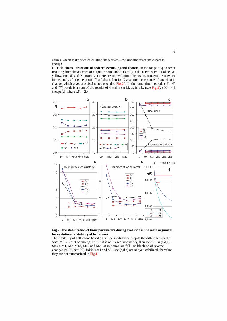
6
causes, which make such calculation inadequate—the smoothness of the curves is
enough.
c – Half-chaos – fractions of ordered events (q) and chaotic. In the range of q an order
resulting from the absence of output in some nodes (k = 0) in the network er is isolated as
yellow. For ‗d‘ and X (from ‗7‘) there are no evolution, the results concern the network
immediately after generation of half-chaos, but for X also after acceptance of one chaotic
change, which gives a typical chaos (see also Fig.2f). In the remaining methods (‗5‘, ‗6‘
and ‗7‘) result is a sum of the results of 4 stable set M, as in a,b, (see Fig.2). s,K = 4,3
except ‗d‘ where s,K = 2,4.
Fig.2. The stabilization of basic parameters during evolution is the main argument
for evolutionary stability of half-chaos.
The similarity of half-chaos based on in-ice-modularity, despite the differences in the
way (‗5‘,‘7‘) of it obtaining. For ‗6‘ it is no in-ice-modularity, then lack ‗6‘ in (c,d,e).
Sets J, M1, M7, M13, M19 and M20 of initiation are full - no blocking of reverse
changes (‗5-7‘, N=400). Initial set J and M1, see (c,d,e) are not yet stabilized, therefore
they are not summarized in Fig.1.
264

7
a - Stability of parameter q (degree of order of the system, the contents of the left peak in
Fig.1) shows lack of moving towards the chaos (smaller q) during the evolution.
b - The average time of five latest explosion to the chaos does not grow. In the chaotic
networks such explosions (Fig.3c) happen almost until the not yet exploded processes
exist.
c - The average size of the ice and of the local clusters. In ‗6‘ there is no ice. 7f has a
specific derogation, but it also stabilizes.
d - The average number of global clusters.
e - The average number local clusters.
f - Average q(t) in sets of J and X, starting after construction of in-ice-modular system
(‗7‘). In this experiment (part of ‗7‘) N=800, tmx=2000, no evolution and M sets. J gives
a typical picture for half-chaotic systems - q quickly stabilizes and is high. X starts after
accumulation one disturbing permanent change, which has given large damage
avalanche. Here q(t) drops up to tmx and probably further, but not for er due to k=0.
5 Short attractor and in-ice-modularity
A more detailed analysis of the mechanisms for maintaining the increased
stability of systems with chaotic parameters has shown that the basic condition
of the statistically significant presence of the left peak in the damage
distribution is a sufficiently short attractor. It allows to limit the number of
different circumstances in which secondary initiations (disturbations) appear in
effect of encountering an input state by a node for which the value of the
function was changed. For one expiration of the damage is relatively probable,
but the fade out of each of the many independent disturbations is practically
impossible.
It was checked by the method ‗6‘ that such the condition is sufficient to obtain a
half-chaos, but the shape of the left peak (Fig.1b) was significantly different
from obtained starting from point attractor (method ‗5‘). Practically it contains
only lack of functional change (A = 0) and therefore such system is not suitable
for modeling the evolution of objects like administrative units, technological
processes, technical constructions and living organisms.
The differences in the half-chaos mechanisms obtained starting from the point
attractor (‗5‘) and from the small attractor (‗6‘) were investigated more in
details. It turned out that the mechanism in the first case is very similar to the
indicated by Kauffman in the vicinity of the phase transition – ―small lakes of
activity in the ice‖ (originally: ―unfrozen islands‖) (Kauffman [12]). Kauffman
calls ice nodes that do not change their state. Starting from the small attractors
(‗6‘) practically does not create ice. Point attractor system is a completely
frozen, disturbation unfreezes small subset of nodes (Fig.2c), and inside it
attractor is usually small. After accumulating such the change, the next
disturbation unfreezes another independent piece (clusters in the figures), and an
image similar to modularity is created. I called it in-ice-modularity. In-ice-
modules are also the classic modules, but this is only one, supporting, but less
important factor. The main property of the in-ice-modules is the activity -
changes of the states of forming them nodes. The ice surrounds them and
isolates from the other in-ice-modules. In-ice-modules are the result of the
265

8
Fig.3. Half-chaos and chaos in the presentation of A(t) from simulation of a full set
of small permanent disturbations.
A - number of the nodes states different than in the not disturbed system. t is a number of
steps of network calculation from damage initiation. The details should be watched in
enough magnification - they were presented on the screen pixels. Showed examples are
typical for all experiments or network types. Here s =4, it indicates level of Derrida
equilibrium near A=290 (see Fig.1a). Typical N = 400, tmx = 1000 is used, so the
rectangle has a dimension of 400*1000 pixels. After each of 1200 initiation A(t) is drawn
with a continuous black line. As can be seen, the transition to chaos in the vicinity
Derrida balance is rapid in several to over a dozen steps, where A increases drastically,
so I call it "explosion." Threshold is here chosen at A=150 which is marked in red. It is
used for q calculation. After the end of initiation set, the red curve q(t) - the share of
processes that in the time t did not cross the threshold, was added to the figure. q=1 for
A=N. Red description of the left has been added for readability. Blue line describe the
share of processes that currently have A = 0, i.e. damage fade out.
a – Half-chaos. The red curve q(t) quickly stabilizes at a high level near q=0.4. (See
Fig.2f.) In the lower part of the graph many trajectories are drawn (there are 476 of
1200). The last explosion occurs at t=18. These, and lot of other data are presented on the
266
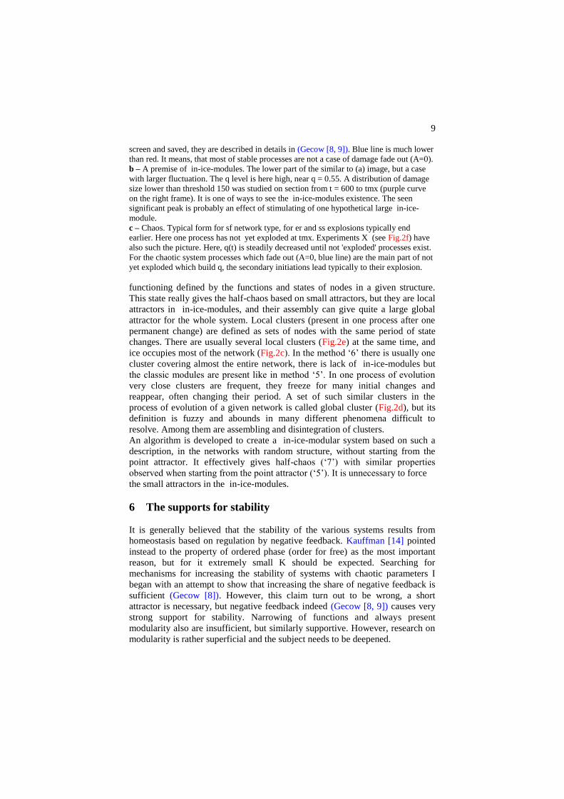
9
screen and saved, they are described in details in (Gecow [8, 9]). Blue line is much lower
than red. It means, that most of stable processes are not a case of damage fade out (A=0).
b – A premise of in-ice-modules. The lower part of the similar to (a) image, but a case
with larger fluctuation. The q level is here high, near q = 0.55. A distribution of damage
size lower than threshold 150 was studied on section from t = 600 to tmx (purple curve
on the right frame). It is one of ways to see the in-ice-modules existence. The seen
significant peak is probably an effect of stimulating of one hypothetical large in-ice-
module.
c – Chaos. Typical form for sf network type, for er and ss explosions typically end
earlier. Here one process has not yet exploded at tmx. Experiments X (see Fig.2f) have
also such the picture. Here, q(t) is steadily decreased until not 'exploded' processes exist.
For the chaotic system processes which fade out (A=0, blue line) are the main part of not
yet exploded which build q, the secondary initiations lead typically to their explosion.
functioning defined by the functions and states of nodes in a given structure.
This state really gives the half-chaos based on small attractors, but they are local
attractors in in-ice-modules, and their assembly can give quite a large global
attractor for the whole system. Local clusters (present in one process after one
permanent change) are defined as sets of nodes with the same period of state
changes. There are usually several local clusters (Fig.2e) at the same time, and
ice occupies most of the network (Fig.2c). In the method ‗6‘ there is usually one
cluster covering almost the entire network, there is lack of in-ice-modules but
the classic modules are present like in method ‗5‘. In one process of evolution
very close clusters are frequent, they freeze for many initial changes and
reappear, often changing their period. A set of such similar clusters in the
process of evolution of a given network is called global cluster (Fig.2d), but its
definition is fuzzy and abounds in many different phenomena difficult to
resolve. Among them are assembling and disintegration of clusters.
An algorithm is developed to create a in-ice-modular system based on such a
description, in the networks with random structure, without starting from the
point attractor. It effectively gives half-chaos (‗7‘) with similar properties
observed when starting from the point attractor (‗5‘). It is unnecessary to force
the small attractors in the in-ice-modules.
6 The supports for stability
It is generally believed that the stability of the various systems results from
homeostasis based on regulation by negative feedback. Kauffman [14] pointed
instead to the property of ordered phase (order for free) as the most important
reason, but for it extremely small K should be expected. Searching for
mechanisms for increasing the stability of systems with chaotic parameters I
began with an attempt to show that increasing the share of negative feedback is
sufficient (Gecow [8]). However, this claim turn out to be wrong, a short
attractor is necessary, but negative feedback indeed (Gecow [8, 9]) causes very
strong support for stability. Narrowing of functions and always present
modularity also are insufficient, but similarly supportive. However, research on
modularity is rather superficial and the subject needs to be deepened.
267

10
7 The basic details of simulations
Simulation studies and their analysis include many important details that are
unfeasible to include in this article. They are described in more than 200 pages
of reports (Gecow [9]), only selected of them in article (Gecow [8]). Only basic
ones are listed here.
The typical size of the studied network is N=400 nodes, but experiments with
N=800 and even 4000 also exist. The basic parameters are: s - the number of
equally probable states of the signal, uniquely s=2 (the Boolean network
denoted by ‗d‘ in Figs.1) or usually s=4; and K - number of inputs to the node,
constant for the whole network, K=4 for s=2 and K=3 for s=4. A(t) - the number
of node states different from the undisturbed pattern at a given moment t is the
principal measured value. This value is shown in Fig.3 and is also used (Figs.2f,
3) to determine q(t). The particular system is calculated at tmx discrete time
steps t after disturbation, and then at t=tmx, more adequate value for the final
results (Fig.1) is recorded as averaged A over the last 50 counting steps t.
Typically, tmx is 1000, but longer stretches are also used, even up to 20000. The
tmx value was arbitrarily determined on the basis of preliminary simulations,
but it is checked whether the increase would not change the results.
Network types sf, ss and er are used in experiments described here. The second
letter indicates the network type in the figures. The number of networks with
parameters type,s,K in a particular final simulation is usually about 600, it
happens 100, but often experiments were repeated in a similar way, giving a
much greater certainty. Due to the strong influence of various factors, often
sporadic, formal errors in the obtained results are not calculated, judging such a
calculation as clearly inadequate and misleading. This problem is limited to the
similarity of results from the similar simulations and the visual evaluation of
fluctuations. The evolution of the experiments ‗5‘, ‗6‘, ‗7‘ has many additional
constraints to increase credibility. They are similar in these three cases for the
basic results, but moreover, a series of simulations of other rules are performed.
After initial set of initiation (J) there are 20 sets M, in most of them the reversal
of the accepted changes are blocked. This results in the exclusion of a large
number of initiations from the measurements and leads to a significant
slowdown of evolution. After several such set, the reversal is allowed (M1, M7,
M13, M19, M20), assuming that the change has already another circumstances.
It also allows to correct measure of various phenomena that illustrate evolution
(Fig.2). Since the attractor is decreasing spontaneously, making it difficult to
move away from the point attractor, it is also forbidden to reduce the global
attractor to less than 7, and in the M20 (at ‗5‘, ‘6‘, ‘7‘) to reduce the attractor.
Also, the point of initiation of damage is shifted by t=50 after each accumulated
change, because the magnitude of this shift turn out to be a significant factor.
268

11
8 Conclusion
Various complex objects adapted by natural selection or humans were attempted
to model by dynamic complex networks. For that, Kauffman's Boolean
networks are perfect. It was estimated that mean connectivity K should be
clearly larger than 2. However, such networks, according to current views,
should be chaotic, and this did not match the features of modeled objects. The
discovery of the half-chaos in which K and s can take larger values than the
extreme 2, and yet in the model remains the order, removed from this modeling
sharp constraints, which until now are the typical basis of many considerations
(Nghe et al. [18], Serra et al. [19, 20], Kauffman [12, 14], Aldana et al. [1, 2],
Luque and Ballesteros [17], Sole et al. [23], Kauffman et al. [15], Shmulevich et
al. [22], Iguchi et al. [10], Villani et al, [25], Kinoshita, [16]). This opens the
door to adequate models with complex networks.
Kauffman's well-known hypothesis (Kauffman [12, 13]) "lives on the edge of
chaos and order" as a result of deepening the model and finding the half-chaos is
here modified to "life evolves in the half-chaos of not fully random systems".
This change entails deeper interpretive conclusions, indicates the natural basis
of the identity of the evolving object and the model of its death necessary for
Darwinian elimination.
Of course, such a brief summary is necessarily a great simplification. Basing the
conclusions on the finite network simulations in complex nonlinear phenomena
is well-justified, but is in conflict with the habit of defining chaos through
Lyapunov exponent, whose analog for networks (coefficient of damage
propagation (Gecow [7]) and eq.2.3 in (Aldana et al. [1])) in the case of half-
chaos turns out to be misleading. The presented results can be treated as a guide
to developing more advanced methods, but in the case of finite, dynamic
complex networks, it will not necessarily be a more comfortable and more
relevant description.
References 1. M. Aldana, S. Coppersmith, L. P. Kadanoff, ―Boolean Dynamics with Random
Couplings‖ in Perspectives and Problems in Nonlinear Science, Applied Mathematical
Sciences Series, ed. E. Kaplan, J. E. Marsden, K. R. Sreenivasan, Springer-Verleg,
Berlin 2003.
2. M. Aldana, Dynamics of Boolean Networks with Scale Free Topology. Physica D 185,
45-66, 2003.
3. A.-L. Barabási, R. Albert, H. Jeong, Mean-field theory for scale-free random
networks. Physica A 272, 173–187, 1999.
4. B. Derrida, Y. Pomeau, Random Networks of Automata: A Simple Annealed
Approximation. Europhys. Lett., 1(2), 45–49, 1986.
5. B. Derrida, G. Weisbuch, Evolution of Overlaps Between Configurations in Random
Boolean Networks. Journal De Physique 47, 1297–1303, 1986.
6. P. Erdős, A. Rényi, Random graphs. Publication of the Mathematical Institute of the
Hungarian Academy of Science, 5, 17–61, 1960.
269

12
7. A. Gecow, Emergence of Matured Chaos During Network Growth, Place for Adaptive
Evolution and More of Equally Probable Signal Variants as an Alternative to Bias p.
in: Chaotic Systems, E.Tlelo-Cuautle (ed.), ISBN: 978-953-307-564-8, 280-310
http://www.intechopen.com, 2011.
8. A. Gecow, Life is not on the edge of chaos but in a half-chaos of not fully random
systems. Definition and simulations of the half-chaos in complex networks,
http://arxiv.org/abs/1712.09609 v3, 2019.
9. A. Gecow, Report of simulation investigations, a base of statement that life evolves in
the half-chaos http://vixra.org/abs/1603.0220 , 2016, with its second part: Report of
simulation investigations, part II, a growth of half-chaotic autonomous networks
http://vixra.org/abs/1711.0467, 2017.
10. K. Iguchi, S. Kinoshita, H. Yamada, Boolean dynamics of Kauffman models with a
scale-free network. J Theor Biol 247; 138–151, 2007.
11. S. A. Kauffman, Metabolic stability and epigenesis in randomly constructed genetic
nets. J. Theor. Biol. 22, 437-467, 1969.
12. S. A. Kauffman, Requirements for Evolvability in Complex Systems - Orderly
Dynamics and Frozen Components. Physica D 42, 135–152, 1990.
13. S. A. Kauffman, The Origins of Order: Self-Organization and Selection in Evolution,
Oxford University Press New York 1993.
14. S.A. Kauffman, At Home in the Universe, Oxford University Press USA 1996.
15. S.A. Kauffman, C. Peterson, B. Samuelsson, C. Troein, Genetic networks with
canalyzing Boolean rules are always stable. PNAS vol. 101 no.49, 17102-17107, 2004.
16 S. Kinoshita, H. Yamada Role of Self-Loop in Cell-Cycle Network of Budding
Yeast. Open Journal of Biophysics, 9, 10-20, 2019
https://doi.org/10.4236/ojbiphy.2019.91002.
17. B. Luque, F.J. Ballesteros, Random walk networks. Physica A 342 207–213, 2004.
18. P. Nghe, W. Hordijk, S. A. Kauffman, S. I. Walker, F. J. Schmidt, H. Kemble, J. A.
M. Yeates, N. Lehman, Prebiotic network evolution: Six key parameters. Molecular
BioSystems, 11(12), 3206-3217. DOI: 10.1039/c5mb00593k , 2015.
19. R. Serra, M. Villani, A. Semeria, Genetic network models and statistical properties of
gene expression data in knock-out experiments. J. Theor. Biol. 227, 149-157, 2004.
20. R. Serra, M. Villani, A. Graudenzi, S. A. Kauffman, Why a simple model of genetic
regulatory networks describes the distribution of avalanches in gene expression data.
J.Theor.Biol, 246 449-460, 2007.
21. H. Schuster, Deterministic Chaos: An Introduction. Physik-Verlag, 1984.
22. I. Shmulevich, S. A. Kauffman, M. Aldana, Eukaryotic cells are dynamically ordered
or critical but not chaotic. PNAS 102 (38), 13439–13444, 2005.
23. R.V. Sole, B. Luque, S. Kauffman, ―Phase transitions in random networks with
multiple states‖, Technical Report 00-02-011, Santa Fe Institute 2000.
24. L. Turnbull, M.T. Hütt, A.A. Ioannides, S. Kininmonth, R. Poeppl, K. Tockner, L.J.
Bracken, S. Keesstra, L. Liu, R. Masselink, A.J. Parsons, Connectivity and complex
systems: learning from a multi-disciplinary perspective, Applied Network Science;
3:11, 2018. https://doi.org/10.1007/s41109-018-0067-2
25. M. Villani, L. La Rocca, S.A. Kauffman, R. Serra, Dynamical Criticality in Gene
Regulatory Networks. Complexity Hindawi, 2018. https://doi.org/10.1155/2018/5980636
270

1
Albert Einstein and the doubling of the deflection of light
Jean-Marc Ginoux1
One of the three consequences of Einstein’s theory of general relativity was the curvature of
light passing near a massive body. In 1911, he published a first value of the angle of
deflection of light, then a second value in 1915, equal twice the first. In the early 1920s, when
he received the Nobel Prize in Physics, a violent controversy broke out over this result. It was
then disclosed that the first value he had obtained in 1911 had been calculated more than a
century before by a German astronomer named Johann von Soldner. The aim of this article is
therefore to compare the methods used by Soldner and then by Einstein leading to this first
value and to explain the importance of the doubling of this value in the framework of
Einstein’s theory of gravitation.
A. The Genesis of General Relativity and the Curvature of Light
Two years after the publication of his article on special relativity, Albert Einstein considered
generalizing his theory. Thus, in 1907, he wrote an article entitled “Relativitätsprinzip und die
aus demselben gezogenen Folgerungen” (“On the Principle of Relativity and the Conclusions
Drawn from it”), at the request of Johannes Stark, editor of the Jahrbuch der Radioaktivität,
in which he presented for the first time one of the consequences of his theory. In paragraph V.
entitled “The Principle of Relativity and Gravitation”, he wrote:
1 Laboratoire des Sciences de l’Information et des Systèmes, LIS, CNRS, UMR 7020 – Archives Henri Poincaré, AHP, CNRS, UMR 7117.
271

2
“From this it follows that those light rays that do not propagate along the -axis
are bent by the gravitational field2…”
At that time Einstein thought that the effect of gravitational field on rays of light was too
weak to be detected as evidenced by his conclusion:
“Unfortunately, the effect of the terrestrial gravitational field is so small according
to our theory (because of the smallness of 2
x
c
) that there is no prospect of a
comparison of the results of the theory with experience3.”
During the autumn 1911, Einstein became full professor of theoretical physics at the
German Charles-Ferdinand University in Prague. Einstein lived more than a year at number 7
Leniscka Street with his first wife Mileva Maric and their two children Hans Albert and
Eduard. Here he wrote a second article, considered as the starting point of his theory of
general relativity: “Einfluss der Schwerkraft auf die Ausbreitung des Lichtes” (“On the
influence of Gravitation on the Propagation of Light”) in which he gave a first value of the
deflection of light passing near a massive body. In paragraph 4 entitled Curvature of light rays
in the gravitational field, he wrote:
“By equation (4) a light-ray passing by a heavenly body suffers a deflection to the
side of the diminishing gravitational potential, that is, to the side directed toward
the heavenly body, of the magnitude
2 Albert Einstein, “Relativitätsprinzip und die aus demselben gezogenen Folgerungen” (“On the Principle of Relativity and the Conclusions Drawn from it”) Jahrbuch der Radioaktivität, 4, 411–462, 1907. 3 Ibid.
272

3
2
2 2 2
2
1 2cos
v
v
kM kMv ds
c r c
,
where k denotes the constant of gravitation, M the mass of the heavenly body, Δ
the distance of the ray from the center of the body (and r and are as shown in
Fig. 3). A light-ray going past the Sun would accordingly undergo deflection by
the amount of 4.10−6 = 0.83 seconds of arc. The angular distance of the star from
the center of the Sun appears to be increased by this amount. As the fixed stars in
the parts of the sky near the Sun are visible during total eclipses of the Sun, this
consequence of the theory may be compared with experimental evidence4.”
Then, he added:
“It would be urgently wished that astronomers take up the question here raised,
even though the considerations presented above may seem insufficiently
established or even bizarre. For, apart from any theory, there is the question
whether it is possible with the equipment at present available to detect an
influence of gravitational fields on the propagation of light5.”
In 1913 Einstein was appointed, on the recommendation of Marie Curie and Henri Poincaré,
to a chair of mathematical physics at the Swiss Federal Polytechnic in Zürich (later the
Eidgenössische Technische Hochschule, ETH) where he had studied a few years earlier. The
following year, he joined Berlin to become director of the Kaiser-Wilhelm Institute of Physics,
4 Albert Einstein, “Einfluss der Schwerkraft auf die Ausbreitung des Lichtes” (“On the influence of Gravitation on the Propagation of Light”), Annalen der Physik, 4(35), 898–908, 1911. 5 Ibid.
273

4
and university professor. On November 1915, he submitted four papers to the journal of the
Prussian Academy of Sciences6. Then, he published in 1916 in Annalen der Physik a 40-page
article entitled “Die Grundlage der algemeinen Relativitätstheorie” (“The Foundations of the
General Theory of Relativity”) considered as the final and complete version of his theory of
general relativity. In the last section he presented the three observable physical consequences
of his theory and in particular the curvature of the light rays and explained that this latter
consequence could be verified by exact astronomical experiments:
“From this it follows that the spectral lines of light reaching us from the surface of
large stars must appear displaced towards the red end of the spectrum*.
*According to E. Freundlich, spectroscopical observations on fixed stars of
certain types indicate the existence of an effect of this kind, but a crucial test of
this consequence has not yet been made7.”
Then, he provided a second value of the deflection of light passing near a massive body:
“We examine the curvature undergone by a ray of light passing by a masse M at
the distance Δ. If we choose the system of co-ordinates in agreement with the
6 Albert Einstein, “Grundgedanken der allgemeinen Relativitätstheorie und Anwendung dieser Theorie in der Astronomie” (“Fundamental Ideas of the General Theory of Relativity and the Application of this Theory in Astronomy”), Preussische Akademie der Wissenschaften, Sitzungsberichte, 315, 1915, “Zur allgemeinen Relativitätstheorie” (“On the General Theory of Relativity”), Preussische Akademie der Wissenschaften, Sitzungsberichte, 778-786 & 799-801, November 4, 1915, “Erklärung der Perihelbewegung des Merkur aus der allgemeinen Relativitätstheorie” (“Explanation of the Perihelion Motion of Mercury from the General Theory of Relativity”), Preussische Akademie der Wissenschaften, Sitzungsberichte, 831-830, November 18, 1915, “Feldgleichungen der Gravitation” (“The Field Equations of Gravitation”), Preussische Akademie der Wissenschaften, Sitzungsberichte, 844-847, November 25, 1915. 7 Albert Einstein, “Die Grundlage der allgemeinen Relativitätstheorie” (“The Foundations of the General Theory of Relativity”), Annalen der Physik, 4(49), 769–822, 1916.
274

5
accompanying diagram, the total bending of the ray (calculated positively if
concave towards the origin) is given in sufficient approximation by8
2
MB
According to this, a ray of light going past the sun undergoes a deflexion of
1.7’’…”
It is very surprising to notice that this second value of the angle of deflection of light provided
by Einstein is equal twice the first. It will be learned some years later that the first value
provided by Einstein in 1911 was in fact identical to that published a century earlier by the
German physicist and astronomer Johann Georg von Soldner9. According to Abraham Pais :
“An Argentinian eclipse expedition which had gone to Brazil in 1912 and which
had the deflection of light on its experimental program was rained out. In the
summer of 1914, a German expedition led by Erwin Freundlich and financed by
Gustav Krupp, in a less familiar role of benefactor of humanity, headed for the
Crimea to observe the eclipse of August 21. (Russian soldiers and peasants were
told by their government not to fear evil omens: the forthcoming eclipse was a
natural phenomenon.). When the war broke out, the party was warned in time to
8 The value 28 K c where K represents the Cavendish’s constant. 9 This fact has been reported since by many historians of science such as Thomas Glick, The Comparative Reception of Relativity, Boston Studies in the Philosophy and History of Science, Vol. 103, Springer Netherlands, Dordrecht, D. Reidel, 1987; Jean Eisenstaedt, « De l’influence de la gravitation sur la propagation de la lumière en théorie newtonienne. L’archéologie des trous noirs », Archive for History of Exact Sciences, Vol. 42 (4), (September 1991), p. 315-386. Jürgen Renn, The Genesis of Relativity, Vol. 1-4, Boston Studies in the Philosophy and History of Science, Vol. 250, Springer Netherlands, Dordrecht, D. Reidel, 2007; Milena Wazeck, On Einstein’s opponents: the public controversy about the theory of relativity in the 1920s, Cambridge; New York: Cambridge University Press, 2014. Nevertheless, neither of these references contains any mathematical analysis nor comparison of Soldner’s and Einstein’s results.
275

6
return and some did so. Those who hesitated were arrested, eventually returned
home safely but of course without results. Frustration continued also after
November 18, 1915, the day on which Einstein announced the right bending of
1”74. […]
An opportunity to observe an eclipse in Venezuela in 1916 had to be passed up
because of the war. Early attempts to seek deflection in photographs taken during
past eclipses led nowhere. An American effort to measure the effect during the
eclipse of June 1918 never gave conclusive results. It was not until May 1919 that
two British expeditions obtained the first useful photographs and not until
November 1919 that their results were formally announced10.”
When the armistice was signed on November 11, 1918, two expeditions were mounted, one to
Sobral in Brazil, led by Andrew Crommelin from the Greenwich Observatory, and one to
Principe Island off the coast of Spanish Guinea, led by Eddington. After the return of the
expeditions, data analysis began. Einstein could not hide his enthusiasm in the expectation of
the results. On September 22, 1919, Hendrik Lorentz sent a telegram to Einstein announcing:
“Eddington found stellar shift at solar limb,
tentative value between nine-tenths of a second and twice that.”
On the afternoon of November 6, 1919, at Burlington House in Piccadilly, the Astronomer
Royal, Sir Frank Dyson, had the honour of presenting the results of the two expeditions. He
described in detail the equipment, the photographs, and the complexities of the computations.
His conclusion, however, was simple.
10 Abraham Pais, Subtle Is the Lord: The Science and the Life of Albert Einstein, Oxford University Press, 1982, p. 304.
276

7
“The results of the expeditions to Sobral and Principe leave little doubt that a
deflection of light takes place in the neighbourhood of the sun and that it is of the
amount demanded by Einstein’s generalized theory of relativity.”
Thus, it was considered that the astronomical observations had ‘‘demonstrated’’ the curvature
of space. The day after, Einstein’s name became legendary. The London Times published an
article entitled “Revolution in Science, New Theory of the Universe, Newtonian ideas
overthrown”. On November 9, 1919, the New York Times published the following article:
“Diversion of light Rays Accepted as Affecting Newton’s Principles11.”
Thus, in 1919 the expedition led by Crommelin and Eddington “confirmed” Einstein’s second
prediction, that is to say, that the value of the deflection of the light passing near the Sun was
equal to 1.7 seconds of arc12. Moreover, the question, which was the subject of intense
controversy, was whether or not Einstein was aware of Soldner’s work when he published his
article in 1911.
B. Controversy around the curvature of light
In the early Twenties, Einstein and his theory of relativity were subject to many attacks of
various natures13. The first, the most odious, had an anti-Semitic character. Then, in 1921,
scientists such as Charles Lane Poor, a professor of astronomy, a specialist in Celestial
11 See Jean-Marc Ginoux, Albert Einstein: a biography through the Time(s), Hermann, Paris, 2016. 12 Eddington’s results for the solar eclipse observation of the apparent displacement of stars of 1919 have been widely disputed by many historians of science. See for example John Earman and Clark Glymour, “Relativity and Eclipses: The British Eclipse Expeditions of 1919 and Their Predecessors,” Historical Studies in the Physical Sciences, Vol. 11, No. 1 (1980), p. 49-85. 13 See Milena Wazeck, On Einstein’s opponents: the public controversy about the theory of relativity in the 1920s, Cambridge; New York: Cambridge University Press, 2014.
277

8
Mechanics at Columbia University, tried to prove that Einstein’s theories of relativity were
false. To this aim he published an article entitled « Is Einstein wrong? – A debate14 ». When
Einstein was invited to the Collège de France in 1922 by Paul Langevin, his theories were
challenged by Édouard Guillaume who had worked with him as a patent examiner at the
Swiss patent office in Bern and had come purposely from Swiss in order to “destroy
relativity”. Indeed, he had published a few weeks beforehand an article entitled: “Y a-t-il une
erreur dans le premier mémoire d’Einstein ?” which let no doubt concerning his intentions15.
Unfortunately, this anti-relativistic attitude was shared by a part of the French scientific
community and more particularly by many Academicians of Sciences. It has been initially
convened that Einstein presents his work at the Academy but some of the members of the
Academy had decided as a protest against his presence to rise and leave the hall as soon as he
entered, Einstein had to renounce16. In August 1922, Einstein, who had received many death
threats, decided to leave temporarily Europe. On October 8, 1922, Albert Einstein and his
second wife Elsa came aboard the S.S. Kitano Maru in Marseille (south France) and reached
then their final destination at Fukuoka in Japan where Einstein gave a lecture at the Daihaku
Theater. On November 15, during a stopover in an hotel of Shanghai, Einstein received a
telegram from Sweden announcing him that he has been awarded the Nobel Prize of Physics
for “his contribution to theoretical physics and more particularly for his discovery of the law
of photoelectric effect” and not for his relativity theories.
This news almost immediately triggered new reactions. Einstein’s most virulent opponent was
the German physicist Philipp Lenard, Nobel Prize in 1905 (the year of the relativity theory)
14 Charles Lane Poor, “Is Einstein wrong? – A debate” in The Forum, June 1924, p. 705-715. 15 Édouard Guillaume, “Y a-t-il une erreur dans le premier mémoire d’Einstein ?” Revue Générale des Sciences Pures et Appliquées, vol. 33, 15 janvier 1922, p. 5-10. 16 See Michel Biezunski, Einstein à Paris, Paris, Presses universitaires de Vincennes, Saint Denis, 1991, p. 26.
278

9
and active proponent of the Nazi ideology. Then, in April 1923 Professors Ernst Gehrcke17 of
Berlin, P. Lenard of Heidelberg, O. E. Westin 18 of Stockholm charged Einstein with
downright plagiarism, saying:
“From these facts the conclusion seems inevitable that Einstein cannot be
regarded as a scientist of real note. He is not an honest investigator.” Thus Westin
protested to the Directorate of the Nobel Foundation against the reward of
Einstein19.”
What were “theses facts” invoked by the three professors against Einstein? The New York
Times of April 13 provides the answer:
“… in 1801 Dr. J. von Soldner, a German physicist of eminence in his day,
actually derived the formula recently used by Einstein. This was 122 years ago.
Einstein never once mentions Soldner in his writings. This is bad enough, but the
worst is yet to come.
It has been shown by Professor Dr. E. Gehrcke, Director of the Imperial Physical
and Technical Institute of Berlin, a position first filled by Helmohltz and by
Professor P. Lenard of Heidelberg, winner of the Nobel Prize in Physics, that
Soldner omitted a certain factor in his formula of l801, which error Einstein also
copied when he appropriated the Einstein-Soldner formula in the Einstein paper
of 1911. In a subsequent paper to the Berlin Academy of Science, 1915, Einstein
17 E. Gehrcke (1878-1960) was a German experimental physicist, Director of the Imperial Institute of Berlin. He was a Privatdozent at the Friedrich-Wilhelms-Universität from 1904 to 1921 and an außerordentlicher Professor (extraordinarius professor) from 1921 to 1946. 18 Oscar Edward Westin (1848-1930) was a Swedish engineer, professor of mechanical engineering at the Royal Institute of Technology in Stockholm. 19 See The New York Times, April 13, 1923. This event is also mentioned in Philipp Frank, Einstein: His Life and Times, New York, A. A. Knopf, 1947, p. 202 and next.
279

10
camouflaged this fraud as best he could, yet could not prevent its discovery and
exposure by Professors Lenard of Heidelberg, Gehrcke of Berlin and Westin or
Stockholm.”
To these three scientists was added the professor Arvid Reuterdahl, Dean of the Engineering
Department of the University of St. Thomas, St. Paul, Minnesota. He sent a letter to the Editor
of The New York Times published on June 3, 1923 and in which he claimed:
“There are two episodes in the Einsteinian development of the bending of light. In
Einstein’s 1911 paper the value of the deflection is given as 0.83 of a second.
Soldner’s value was 0.84 of a second. The two formulae are identical except in
the matter of the convenient substitution by Einstein of different letters than those
used by Soldner. Compared, letter for letter, the meanings are, however identical20.
In his 1916 paper Einstein modified his 1911 value to read 1.7 of a second.
Einstein has never taken the world into his confidence concerning the reason of
this change. He has never admitted that either one or the other of these values
must be erroneous21.”
Indeed, in 1916, in his famous article entitled “The Foundations of the General Theory of
Relativity22”, Einstein realized that his earlier result on the bending of light, he had presented
in his previous article of 1911, was too small by a factor of 2. This factor will be proved to be
decisive because it enables to reveal a strict separation between Newtonian and Einsteinian
theory of gravitation. This was due to the fact that in his 1911 paper Einstein had not taken
20 See § C.3. 21 We will see in § C.4 that this statement is partially inaccurate. 22 Albert Einstein, “Die Grundlage der allgemeinen Relativitätstheorie” (“The Foundations of the General Theory of Relativity”), Annalen der Physik, 4(49), 769–822, 1916.
280

11
into account in his computations the curvature of space but, only included the effect of
Newtonian gravitational interaction on the four-dimensional space-time that he will express
later in a Minkowskian metric. According to Abraham Pais :
“Let us briefly recapitulate Einstein's progress in understanding the bending of
light.
1907. The clerk at the patent office in Bern discovers the equivalence principle,
realizes that this principle by itself implies some bending of light, but believes that
the effect is too small to ever be observed.
1911. The professor at Prague finds that the effect can be detected for starlight
grazing the sun during a total eclipse and finds that the amount of bending in that
case is 0’’87. He does not yet know that space is curved and that, therefore, his
answer is incorrect. He is still too close to Newton, who believed that space is flat
and who could have himself computed the 0’’87 (now called the Newton value)
from his law of gravitation and his corpuscular theory of light.
1912. The professor at Zurich discovers that space is curved. Several years pass
before he understands that the curvature of space modifies the bending of light.
1915. The member of the Prussian Academy discovers that general relativity
implies a bending of light by the sun equal to 1’’74, the Einstein value, twice the
Newton value. This factor of 2 sets the stage for a confrontation between Newton
and Einstein23.”
23 Abraham Pais, op. cit., p. 303.
281

12
C. Comparison of the work of Einstein and Soldner
Such a comparison has been subject to many studies and several historians of science have
analyzed both works of Soldner and Einstein from a mathematical point of view during these
last decades. In 1975, Hans Fuchs published an article entitled “On the history of ideas about
the effect of gravity on the light24” in which he presented the proofs leading to the value of the
deflection of light passing near a massive body obtained by Soldner in 1801 and then by
Einstein in 1911 and finally in 1915. After comparing Einstein’s paper of 1911 with that of
Soldner of 1801, Fuchs wrote: “Man erhält also trotz Zuhilfenahme des Aquivalenzprinzips
wieder den alten falschen klassischen Wert! Wie ist das möglich?25”. Then, he explained:
“Obwohl wir von der Erde aus eine Verlangsamung der Vorgänge feststellen, werden wir
doch mit gleichen Uhren auf der Sonne wie auf der Erde die gleichen Frequenzen und die
gleiche Lichtgeschwindigkeit messen, weil die Uhren in gleichem Masse wie die
Naturvorgänge verlangsamt werden!
Diese logisch einwandfreie Sicht der Dinge erlangte Einstein erst durch das tiefere
Verständnis, das durch die allgemeinen Relativitätstheorie gebracht wurde (nach 1915)26.” By
using the Fields Equations of Gravitation and the Schwarzchild metric (including the so-
called Ricci tensors) Fuchs showed that Einstein was then able to give the “der korrekte
relativistische Wert” (“the correct relativistic value”). He also compared the relativistic and
classical calculations and stated that the two results differ by a factor of two. However, his
proof is different from those presented in this paper.
24 Hans Fuchs, “Zur Geschichte der Ideen über die Wirkung der Schwerkraft auf das Licht,” Orion, Vol. 33 (151), (December 1975), p. 183-193. 25 “Thus, despite the aid of the principle of equivalence, one gets the old false classic value again! How is that possible?” 26 “Although we observe a slowing down of the earth from the earth, we will measure the same frequencies and the same speed of light with the same clocks on the sun as on the earth, because the clocks are slowed down to the same extent as the natural processes! Einstein achieved this logically correct view of things only through the deeper understanding that came with the general theory of relativity (after 1915).”
282

13
In 1978, Stanley Jaki published an article in which he recalled the historical context of the
bending of light27. Starting from the seminal works of Newton and Laplace, he presented the
controversy triggered out by Lenard, Gehrcke and Westin (see § B. above). Then, he proposed
an English translation of Soldner’s article allowing historians of science to study and compare
his works with those of Einstein28. He gives many details and references concerning Soldner’s
life but didn’t provide any mathematical analysis of his article.
In 1980, John Earman and Clark Glymour published a long article in which they compared
Einstein’s results of 1911 and 1915. As Fuchs29, they recalled: “Einstein had not by 1911 yet
absorbed the four-dimensional geometrical way of viewing space-time urged by Minkowski.
In certain respects his thinking about space-time was still classical30.” Then, they explained:
“Einstein gave two arguments for the deflection of light passing near a massive body such as
the sun; one argument, given in 1911 before the general theory was in hand, relied on his
“principle of equivalence,” while the other, given in 1916, used Einstein’s own approximate
solution to his gravitational field equations together with Huygens’ principle from classical
optics. The former derivation gave a value for the deflection at the limb of the sun of 0.83" of
arc, the latter 1.7" of arc.” They concluded that: “By 1916 Einstein had obtained two different
expressions for the angular deflection of a light ray by a massive gravitational source, both
giving the angle as a hyperbolic function of distance of closest approach to the massive body.
The two expressions, one from the principle of equivalence and the other from the general
theory, differ only by a factor of two.” Nevertheless, they didn’t compare Einstein’s results
with Soldner’s.
27 See also Jean Eisenstaedt, « De l’influence de la gravitation sur la propagation de la lumière en théorie newtonienne. L’archéologie des trous noirs », Archive for History of Exact Sciences, Vol. 42 (4), (September 1991), p. 315-386. 28 Stanley L. Jaki, “Johann Georg von Soldner and the gravitational bending of light, with an English translation of his essay on it published in 1801,” Foundations of Physics, December 1978, Vol. 8, Issue 11-12, p. 927-950. 29 Hans Fuchs, “Zur Geschichte der Ideen über die Wirkung der Schwerkraft auf das Licht,” Orion, Vol. 33 (151), (December 1975), p. 183-193. 30 John Earman and Clark Glymour, “Relativity and Eclipses: The British Eclipse Expeditions of 1919 and Their Predecessors,” Historical Studies in the Physical Sciences, Vol. 11, No. 1 (1980), p. 49-85.
283

14
In 1981, Hans-Jürgen Treder and Gerhard Jackisch published an article in which they
considered that “A factor 2, which had been the occasion for misinterpretation, has to be
attributed to the terminology used by German physicists and astronomers of that time31.”
They concluded that: “Soldner did nowhere draw false inferences but fell a victim to the
printer’s devil, and it is indisputable that Soldner obtained the Newtonian value of the
deflection of light, which with respect to the constants of his times amounts to 0''84, and not
to Einstein’s value.” Nevertheless, it is obvious that they compared Soldner’s result with that
provided by Einstein in 1915 and not with that of 1911. Moreover, their conclusion has been
challenged by historians of science such as Ledo Stefanini32 who wrote: “Some scholars
attribute the numerical errors appearing in Soldner’s memoir (correctly pointed out by Lenard
in 1921 republication) to typographical errors33, but this does not suffice to clear the issue.”
So, the aim of this work is to mathematically compare the formula obtained by Soldner with
the one stated by Einstein in his paper of 1911 and to verify if they are identical or not. By
using a simple first-order series expansion, it will thus be proved (to our knowledge for the
first time) that both Soldner’s and Einstein’s formula are perfectly identical. Then, a
mathematical analysis of the second formula concerning the bending of light established by
Einstein in 1915 will enable to explain the importance of the doubling of this value in the
framework of Einstein’s theory of gravitation.
31 Hans-Jürgen Treder and Gerhard Jackisch, “On Soldner’s value of Newtonian deflection of light,” Astronomische Nachrichten, Vol. 302 (6), (May 1981), p. 275-277. 32 Ledo Stefanini, “A misunderstanding in Soldner’s interpretation of the gravitational deflection of light,” Lettera Matematica, Vol. 4 (3-4), (March 2017), p. 167-172. 33 Stefanini quotes Hans-Jürgen Treder and Gerhard Jackisch.
284

15
1. Value of deflection of light by Soldner in 1801
Johann Georg von Soldner (1776-1833) was a German physicist, mathematician and
astronomer. He first worked in the Berlin Observatory (Berliner Sternwarte) and later in 1808
in Munich where he became a member of the Academy of Sciences and the director of the
observatory in Bogenhausen. In a paper written in March 1801 and published in 1804, he
calculated the amount of deflection of a light ray by a star based on Newton‘s corpuscular
theory of light and wrote:
“It is, of course, true that already through observations and otherwise one was
aware of considerable deviations from an assumed law; such as was the case with
the aberration of light. There can, however, be deviations which are so small that
it is difficult to decide whether they are true deviations or errors of observation.
There can also be deviations which are considerable but, being combined with
magnitudes one has not yet succeeded in clearly identifying, escape the observer.
Of the latter kind may be the deviation of a light ray from straight line when it
passes close by a celestial body and is considerably exposed to its attraction34.”
Soldner then presented the following diagram (see Fig. 1).
34 See J. von Soldner, “Ueber die Ablenkung eines Lichtstrals von seiner geradlinigen Bewegung,” (“On The Deviation Of A Light Ray From Its Motion Along A Straight Line Through The Attraction Of A Celestial Body Which It Passes Close By”), Berliner Astronomisches Jahrbuch, 1804, p. 161-172. See also Stanley L. Jaki, “Johann Georg von Soldner and the gravitational bending of light, with an English translation of his essay on it published in 1801,” Foundations of Physics, December 1978, Vol. 8, Issue 11-12, p. 927-950.
285

16
Fig. 1. Soldner’s diagram for deflexion of a light ray.
Then, he indicated that “C (Fig. 1) is the center of the attracting body, A is the location at its
surface. From A, a light ray goes into the direction AD or in the horizontal direction, by a
velocity with which it traverses the way v in a second. Yet the light ray, instead of travelling
at the straight line AD, will forced by the celestial body to describe a curved line AMQ,
whose nature we will investigate (…) g be the gravitational acceleration at the surface of the
body. Furthermore CP = x, MP = y and the angle MCP .” Then, he explained:
“The force with which the light ray at M will be pulled by the body in the
direction MC, will be 22gr . This force can be decomposed into two others,
2
2gcos
r and 2
2gsin
r according to the directions x and y; and therefore one
obtains the following two equations (s. Traité de mécanique céleste par Laplace,
Tome I, p. 21)
286
17
2
2 2
2d x gcos
dt r
2
2 2
2d y gsin
dt r …”
These two equations correspond to the projection along the x and y directions of Newton’s
second law according to which the product of the mass by the acceleration (left hand side) is
equal to Newton’s gravitational force (right hand side).
Soldner’s simplification of the “mass of a ray of light” on either side of this equality is
consistent with Newton’s theory of light then considered as made up of small discrete
particles called “corpuscles”. Indeed, it is only in 1803, three years after the writing of
Soldner’s article, that Thomas Young (1773-1829) performed his famous double-slit
experiment from which he proposed a wave theory of the light. Thus, starting from the two
preceding equations and after a demonstration which does not present any great difficulties,
Soldner draws the following conclusion:
“The light ray, however, comes in the direction DA to the eyes of the observer;
thus ADB will be the angle of perturbation. If one calls this angle ω then one has,
since the triangle ABD at A is a right triangle
tanAB
AD
If one puts these values for AB and AD in the expression for tan ω, then one has
287

18
2
2tan
4
g
v v g
If one substitutes in the formula for tan ω the acceleration of gravity on the
surface of the sun, and one takes the radius of that body for unity, then one finds
ω = 0’’.84. If one could observe the fixed stars very close to the sun, then one
would have to take this very much into account. But since this is not known to
happen, the perturbation caused by the sun can also be neglected35.”
At the time, such observations were impossible; Soldner therefore concluded that these effects
were minute. He ended his article as follows:
“Hopefully, no one would find it objectionable that I treat a light ray as a heavy
body. That light rays have all the absolute [basic] properties of matter one can see
from the phenomenon of aberration which is possible only because light rays are
truly material. And furthermore, one cannot think of a thing which exists and
works on our senses that would not have the property of matter36.”
Thus, it appears that Soldner based his computations on the Newton’s emission theory,
according to which light is made up of particles. As far as Einstein is concerned, he made use
of the Huygens principle, that is to say, the variation of the direction of the wavefront as a
function of the luminous frequency, as will be seen in the next section.
35 Ibid. 36 Ibid.
288

19
2. Value of deflection of light by Einstein in 1911
In his 1911 paper, Einstein first established that “the velocity of light in the gravitational field
is a function of the location37.” Then, by using Huygens’s principle, he stated that “light-rays
propagated across a gravitational field undergo deflection38.”
Fig. 2. Einstein’s diagram for deflexion of a light ray.
From this figure (see Fig. 2), Einstein stated that the direction of the wave front changes by an
amount equal to c n per unit of distance along the direction of the wave (where c is the
velocity of light) and the “angle of deflection per unit of path of the light-ray is 1 c
c n
”.
Finally, he obtained “for the deflection , which a light-ray experiences toward the side n
on any path (s) the expression
2
1ds
c n
”
37 Albert Einstein, “Einfluss der Schwerkraft auf die Ausbreitung des Lichtes” (“On the influence of Gravitation on the Propagation of Light”), Annalen der Physik, 4(35), 898–908, 1911. 38 Ibid.
289

20
where the integral goes from to and kM r is the gravitation potential. Then,
Einstein changed variables to polar coordinates as highlighted on the following figure (see Fig.
3a). In order to simplify the understanding of his approach, let’s pose in what follows: n y ,
s x et S R (see Fig. 3b)39.
(a) (b)
Fig. 3. Deflection of a light ray in polar coordinates.
According to Fig. 3b, we have 2 2r x y . Thus, the gravitation potential reads:
2 2
kM
x y
It follows that 32 2
kM kMy
n y y rx y
. Einstein then considers that nearly all of
the deflection occurs within some reasonable proximity of the gravitating body. So, we can
simply set y = R in the integral which reads:
39 See also Kevin Brown, Reflections on Relativity, lulu.com, Mars 2017.
x
y
R
r
290

21
2 3 2 3
1 1kM kMRyds dx
c r c r
.
The following variable changes x R tan , y R leads Einstein to:
2 22
3 2 3 22 2 2 22 2 2 2 22 2
1 2Rd coskMR kMR kM kMdx cos d
c c c R c Rx y R tan R
Then, Einstein ended his 1911 paper by this sentence:
“A light-ray going past the Sun would accordingly undergo deflection by the amount of 4.10−6
= 0,83 seconds of arc40.”
Let’s notice that although the reasonings and the computations are different, the result of
Einstein is exactly the same as that of Soldner (as shown in the next section). In other words,
a light ray passing near the sun will undergo a deflection of nearly 0.83’’.
3. Comparison of Einstein and Soldner formulas
This section aims to prove that both formulas established by Soldner in 1801 and Einstein in
1911 are identical except in the choice of letters.
Soldner’s formula of 1801 reads: 2
2tan
4
g
v v g
- g is the gravitational acceleration at the surface of the body
- v is its velocity. 40 Ibid.
291

22
In his article, Soldner wrote:
“On the presupposition that light needs 564’’.8 decimal seconds of time to come
from the sun to the earth, one finds that it traverses in one-tenth of a second
15.562085 earth radii. Thus v = 15.562085. If one takes among the geographical
latitudes that whose square of the sine is 1/3 (corresponding to a latitude of
35°16’), the earth’s radius as 6,369,514 meters, and the acceleration of gravity
there as 3.66394 meters (see Traité de mécanique céleste by Laplace, Vol. I, p.
118), then expressed in earth radii g = 0.000000575231.”
We deduce that the dimension of the acceleration of gravity on the surface of the body g is s−2
and that of the velocity is s−1. Indeed, Soldner made use of a kind of “normalisation” of these
two physical variables which can be written as 0g g and v c where is the radius
of the considered body (in this case the Sun). Soldner’s formula can be rewritten as
1
2
2 2 22
2
2 2 1 2 4tan 1
44 1
g g g g
v v vgv v gv
But since, according to Soldner g << v, a first-order41 series expansion can be made and reads:
1
24
2 2 2 2 2
2 4 2 4 2tan 1 1
g g g g gO v
v v v v v
41 In his 1911 and 1915 articles Einstein also made use of first-order approximations.
292

23
The angle is considered as infinitely small, so we deduce that 2
2g
v .
Then, by posing 0g g and v c , we have:
02
2g
c
In 1911, Einstein proposed the following formula: 2
2kM
c
where
- k is the constante of gravitation (Cavendish’s constant),
- M is the mass of the heavenly body,
- is the distance of the ray from the center of the body, i.e., its radius.
In the case of the Sun, we have: 0 2
kMg
. So, it gives
02 2 2 2
22 2 gkM kM
c c c
Thus, both Soldner and Einstein’s formulas are identical.
02
2g
c
293

24
4. Value of deflection of light by Einstein in 1915
During the autumn 1915, Einstein completed his general theory of relativity. He thus modified
his gravitation potential while taking into account as previously the Newton’s gravitational
interaction (see § C.2) but also the curvature of space near a massive body42. Then, he
expressed the gravitation potential as
2
3 22 2 2 2
kM mx
x y x y
In this case
2 2 2
3 2 52 2 2 2
4kM kMx x ykMy
n y y rx y x y
The integral reads then 2 2 2 2
2 5 2 5
1 4 4x y kMR x RkMyds dx
c r c r
. By using the same
variable changes, x R tan , y R , Einstein obtained:
2 22 2 3
52 5 2 2 22
4 14 4tankMR x R kMR Rd kMdx
c r c cos c RR cos
42 Cf. Kevin Brown, Op. Cit.
294

25
In his publication of 1916 Einstein43 provided for the deflection of a light ray the value
2
MB
which results of the previous integration. He defined at the page 818 of this same
article the constant 2
8 k
c
(see Eq. (69)). By replacing into the value of B, we have:
2
42
kMB
c R
Einstein wrote in his conclusion:
“According to this, a ray of light going past the sun undergoes a deflexion of 1.7’’…”
Thus, it appears that Einstein’s computation of the value of deflection of a light ray performed
in 1915 led him to twice the amount derived in his 1911 paper.
Where does this doubling come from? How did Einstein justify it?
In fact, contrary to what Arvid Reuterdahl (see § B) claimed, Einstein has really “taken the
world into his confidence concerning the reason of this change”. Indeed, as early as 1915,
Einstein wrote:
“By use of the Huygens principle, one finds through a simple calculation, that a
light ray from the Sun at distance undergoes an angular deflection of
magnitude 2 , while the earlier calculation had given the value . A
43 Albert Einstein, “Die Grundlage der allgemeinen Relativitätstheorie” (“The Foundations of the General Theory of Relativity” ), Annalen der Physik, 4(49), 769–822, 1916.
295

26
corresponding light ray from the surface rim of the Sun should give a deviation of
1.7’’ (instead of 0.85’’) 44.”
In 1920, in the appendix 3 of the third edition of his book written in 1916, he wrote:
“As a result of this theory, we should expect that a ray of light which is passing
close to a heavenly body would be deviated towards the latter. For a ray of light
which passes the sun at a distance of sun-radii from its centre, the angle of
deflection ( ) should amount to
1.7 seconds of arc
It may be added that, according to the theory, half of this deflection is produced
by the Newtonian field of attraction of the sun, and the other half by the
geometrical modification (“curvature”) of space caused by the sun45.”
D. Conclusion
The author of one of Einstein’s most famous biographies, Ronald Clark had written that he
was “the man who had bent the light”. One would be led to believe that the concept of
“curvature of light” which was conceived by Soldner in the early nineteenth century was
rediscovered a century later by Einstein. In fact, many authors have shown that this idea was
44 Albert Einstein, “Erklärung der Perihelbewegung des Merkur aus der allgemeinen Relativitätstheorie” (“Explanation of the Perihelion Motion of Mercury from the General Theory of Relativity”), Preussische Akademie der Wissenschaften, Sitzungsberichte, 831–839, 1915. 45 Albert Einstein, Relativity: The Special and General Theory, London, Methuen & Co Ltd, 1920.
296

27
already present in the works of Isaac Newton. Indeed, in the first of the famous Queries of his
work entitled Opticks, Newton wrote in 1704:
« Do not Bodies act upon Light at a distance, and by their action bend its Rays, and is not this
action (caeteris paribus) strongest at the least distance? »
It thus appears that neither Soldner nor Einstein is the inventor of the concept of “curvature of
light”. One can then ask whether Einstein had any knowledge of Soldner's work. It is
naturally very difficult to answer this question. The elements we have today allow us only to
affirm that the values of the deflection of light rays passing near a massive body obtained by
Soldner in 1801 and by Einstein in 1911 are perfectly identical, although the computations of
Soldner were based on Newton’s corpuscular theory, while those of Einstein were based on
the Huygens’s principle. First, it is important to note that the impossibility of measuring the
deflection of light during the eclipses of 1912 and 1914 was an extraordinary opportunity for
Einstein. Indeed, without this providential rain and without the declaration of war the
observations of the astronomers would have absolutely not confirmed the first value that it
had provided in 1911 and they would certainly have invalidated his theory.
Note then that the method of computing the deflection of light that Einstein used in 1915 is
exactly the same one he used in 1911. The only difference is the expression of gravitation
potential which took into account the curvature of the space in the vicinity of a massive body.
Thus, in his article in 1915, Einstein provided a value (1.7’’) which was well contained within
the range of values observed by the expeditions led by Crommelin and Eddington in 1918
(0.9’’ to 1.8’’). It is clear from this analysis that the plagiarism accusations against Einstein
which are part of an anti-relativist and anti-Semitic movement are absolutely baseless. Even if
it has been established that the values of the deflection of a light ray provided by Soldner in
297

28
1801 and Einstein in 1911 are identical, they are both wrong because they don’t take into
account the curvature of space and so, are not consistent with those “obtained” by Crommelin
and Eddington and confirmed after by more accurate astronomical observations.
E. References
Michel Biezunski, Einstein à Paris, Paris, Presses universitaires de Vincennes, Saint Denis,
1991.
Kevin Brown, Reflections on Relativity, lulu.com, Mars 2017.
Ronald W. Clark, Einstein the life and times, London, Hodder and Stoughton, 1973, p. 494.
John Earman and Clark Glymour, “Relativity and Eclipses: The British Eclipse Expeditions of
1919 and Their Predecessors,” Historical Studies in the Physical Sciences, Vol. 11, No. 1
(1980), p. 49-85.
Jean Eisenstaedt, « De l'influence de la gravitation sur la propagation de la lumière en théorie
newtonienne. L'archéologie des trous noirs », Archive for History of Exact Sciences, Vol. 42
(4), (September 1991), p. 315-386.
Albert Einstein, “Relativitätsprinzip und die aus demselben gezogenen Folgerungen” (“On the
Principle of Relativity and the Conclusions Drawn from it”) Jahrbuch der Radioaktivität, 4,
411–462, 1907.
298

29
Albert Einstein, “Einfluss der Schwerkraft auf die Ausbreitung des Lichtes” (“On the
influence of Gravitation on the Propagation of Light”), Annalen der Physik, 4(35), 898–908,
1911.
Albert Einstein, “Erklärung der Perihelbewegung des Merkur aus der allgemeinen
Relativitätstheorie” (“Explanation of the Perihelion Motion of Mercury from the General
Theory of Relativity”), Preussische Akademie der Wissenschaften, Sitzungsberichte, 831–839,
1915.
Albert Einstein, “Die Grundlage der allgemeinen Relativitätstheorie” (“The Foundations of
the General Theory of Relativity” ), Annalen der Physik, 4(49), 769–822, 1916.
Albert Einstein, Relativity: The Special and General Theory, London, Methuen & Co Ltd,
1920.
Philipp Frank, Einstein: His Life and Times, New York, A. A. Knopf, 1947
Hans Fuchs, “Zur Geschichte der Ideen über die Wirkung der Schwerkraft auf das Licht,”
Orion, Vol. 33 (151), (December 1975), p. 183-193.
Thomas Glick, The Comparative Reception of Relativity, Boston Studies in the Philosophy
and History of Science, Vol. 103, Springer Netherlands, Dordrecht, D. Reidel, 1987;
Jaume Giné, “On the origin of the deflection of light,” Chaos, Solitons & Fractals, 2008, vol.
35(1), p. 1-6.
299

30
Jean-Marc Ginoux, Albert Einstein : une biographie à travers le temps, Hermann, Paris, 2016.
Jean-Marc Ginoux, Albert Einstein: a biography through the time(s), Hermann, Paris, 2016.
Édouard Guillaume, « Y a-t-il une erreur dans le premier mémoire d’Einstein ? » Revue
Générale des Sciences Pures et Appliquées, vol. 33, 15 janvier 1922, p. 5-10.
Stanley L. Jaki, “Johann Georg von Soldner and the gravitational bending of light, with an
English translation of his essay on it published in 1801”, Foundations of Physics, December
1978, Vol. 8, Issue 11-12, p 927-950.
Charles Lane Poor, « Is Einstein wrong? – A debate » in The Forum, June 1924, p. 705-715.
Abraham Pais, Subtle Is the Lord: The Science and the Life of Albert Einstein, Oxford
University Press, 1982.
Jürgen Renn, The Genesis of Relativity, Vol. 1-4, Boston Studies in the Philosophy and
History of Science, Vol. 250, Springer Netherlands, Dordrecht, D. Reidel, 2007
Johann von Soldner, “Ueber die Ablenkung eines Lichtstrals von seiner geradlinigen
Bewegung,” (“On The Deviation Of A Light Ray From Its Motion Along A Straight Line
Through The Attraction Of A Celestial Body Which It Passes Close By”), Berliner
Astronomisches Jahrbuch, 1804, p. 161-172.
300

31
Ledo Stefanini, “A misunderstanding in Soldner’s interpretation of the gravitational deflection
of light,” Lettera Matematica, Vol. 4 (3-4), (March 2017), p. 167-172.
Hans-Jürgen Treder and Gerhard Jackisch, “On Soldner’s value of Newtonian deflection of
light,” Astronomische Nachrichten, Vol. 302 (6), (May 1981), p. 275-277.
Milena Wazeck, On Einstein’s opponents: the public controversy about the theory of
relativity in the 1920s, Cambridge; New York: Cambridge University Press, 2014.
301

302

A Statistical Ensemble Based Approach forEntropy in Cryptocurrencies Markets
Luca Grilli1 and Domenico Santoro2
1 Universita degli Studi di Foggia, Dipartimento di Economia, Management eTerritorio, Via Da Zara, 11, I-71121 Foggia, Italy(E-mail: [email protected])
2 Universita degli Studi di Foggia, Dipartimento di Economia, Management eTerritorio, Via Da Zara, 11, I-71121 Foggia, Italy(E-mail: domenico [email protected])
Abstract. In this paper, we point out an “affinity” between the system of agentstrading in cryptocurrencies and statistical mechanics. In particular, we try to extendthe concept of entropy in the sense of Boltzmann such a definition to a model inwhich the particles are replaced by N economic subjects (agents), that are completelydescribed by their ability to buy and to sell a certain quantity of cryptocurrencies.In addition, by applying this model to the closing prices of some of this we show thatentropy can be used as an indicator to forecast the price trend of cryptocurrencies.Keywords: Cryptocurrency, Entropy, Prices Forecast, Boltzmann, Blockchain.
1 Introduction
The concept of entropy was first introduced by Clausius[23], whose definitionwas applied to a thermodynamic system that performs a transformation. Sincethe mid-19th century, entropy has been a key element linking mechanics tothermodynamics; however, this entropy suffered from a conceptual problemwhich, as demonstrated by Gibbs[28], was revealed in the case of identical gases(Gibbs Paradox ). He solved this problem by changing the count of states. Onthe other hand, Boltzmann[16] presented his statistical interpretation of ther-modynamic entropy, managing to link the macroscopic properties of a systemwith the microscopic ones. Based on Gibbs, in 1949 Shannon[8] developed atheory capable of evaluating the amount of information that is lost in receivinga message from a source to a recipient. This form of entropy was generalizedby Renyi[3], Tsallis[7], Adler et al.[15] (in topology), redefined by Pincus[19](approximate entropy) and - more recently - by Chen et al.[27] as a time seriesregularity measure.The application of entropy in sectors such as economics or finance is linked tothe work of Brissaud[4] that assimilated entropy to disorder, so as to make thistool that has always been applied the physics part of the economy. The formsof entropy most used in this case are Shannon entropy and the generalizationsby Renyi and Tsallis, who contributed to creating a new line of application forthe management of financial portfolios. For example, these new types of en-tropy has been used by Philippatos and Wilson[6], Usta and Kantar[10], Janaet al.[22], Gulko[17], and Dionisio et al.[2].What we want to demonstrate in this paper is that it is possible to assimilate
303

a cryptocurrency system to a thermodynamic system. In this way, we are ableto determine entropy in the sense of Boltzmann so that we can make pricepredictions related to the possibility that they move in a more or less widerange; unlike all the recent applications concerning theories based on Shannonentropy and its derivations. Innovation is linked to the reinterpretation of themonetary system of cryptocurrencies. In this sense, we can apply physical the-ories to a social science. Once the system has been described, our goal is toverify that entropy calculated in the physical sense also occurs in the economiccontext to allow us to make assumptions on how the process could move in thenext future. This type of conjecture has been presented by Sergeev[20], Zakiraset al.[26] and Smith and Foley[9]. In particular McCauley[13], based on thisprevious theory, maintains that the illiquidity of the markets does not allow forthe application of the concepts of statistical mechanics.The paper structure is the following: in Section 2 we analyze cryptocurren-cies and their key characteristics, focusing on the fact that they have a supplylimit; in Section 3 we describe the evolution of a system of a particle in statis-tical thermodynamics and how to determine its entropy, subsequently applyingthese notions to our monetary system; in Section 4 we define the theoreticalassumptions we can link to the system created previously to study the priceevolution in these currency markets and we analytically describe the calculationof entropy using real data; finally in section 5 some conclusions are drawn.
2 Cryptocurrency
Cryptocurrencies represent a digital currency system with no guarantee institu-tion and no transaction control. The main cryptocurrencies, by media coverageor by the possibility that some financial intermediaries offer to use them as apayment instrument, are: Bitcoin, Ethereum and Ripple. Unlike traditionalfinancial assets, their value is not based on tangible assets such as the economyof a country or a company, but it is based on the security of an algorithm thattracks transactions. Their definition is controversial since by some entities [11]they are considered intangible assets (IFRS) while according to the Germanfinancial supervisory authority (BaFin) they are officially financial instruments[5]. All the cryptocurrencies have been based on the Bitcoin, a currency cre-ated by Nakamoto[24] who in 2009 released a software capable of implementingtransactions. The currency itself is a unique alphanumeric string that repre-sents a certain transaction, a transaction which will then be entered in a publicregister called blockchain.The blockchain is the fulcrum of these systems and is essentially a register inwhich the data of the owners of the currency are entered, transactions occurin an encrypted manner. The blockchain is a data structure consisting of alist of transaction blocks linked together so that each refers to the previousone in the chain. A block is a data structure that aggregates transactions toinclude them in the public register. The block is made of a header, containingmetadata, followed by a long list of transactions. A complete block, with alltransactions, is, thus, 1000 times larger than the block header [1]. The in-tegrity of the blockchain network is guaranteed through consensus algorithms
304

such as Proof-of-Work (PoW) and Proof-of-Stake (PoS), that solve the Byzan-tine Generals Problem[12] (problem of consent in the presence of errors). Aconsensus algorithm is a mechanism used by the network to reach consensus,i.e. ensuring that the protocol rules are followed and that transactions occurcorrectly so that coins can only be spent once.The cryptocurrency generation process is called mining, which adds money tothe supply. Cryptocurrencies are “minted” during the creation of each block ata fixed and decreasing rate [1]: each block generated on average every 10 min-utes contains new currency. For example, if we consider Bitcoin, every 210000blocks the currency issue rate decreases by 50% (the availability of new coinsgrows as a geometric series every 4 years). It is estimated that around theyear 2140, the production of the last block will be reached (6930000) and thenumber of coins produced will tend to its upper limit of 21 million (precisely20999999.97690000), value introduced by Nakamoto himself and contained inthe variable “MAX MONEY” as can be read in the source code present onGitHub. This value represents a sanity check, especially used to avoid bugs inwhich it is possible to generate currency from nothing and therefore movingtowards a situation in which the blockchain diverges into different potentialpaths (called fork).
3 Methodology
The main assumption in this paper is that the prices of cryptocurrencies behavelike a thermodynamic system, so it is possible to determine entropy by usingthe Boltzmann formula. In order to present the theoretical framework and themethodology, we need to briefly introduce the main physical results. In Statis-tical Mechanics a macroscopic system is made up of N molecules (N ∼ 1024
is the Avogadro’s constant) whose mechanics provide the evolution of 6N dy-namic variables describing completely the microscopic states of this system.Motion in the phase space can be studied using the 3N position componentsand the 3N momenta components, indicated with qi and pi whose evolu-tion is driven by Hamilton’s equations. Mechanics, therefore, provides a verydetailed description of the system contrary to thermodynamics which studiesthe collective variations; for this reason, the mechanical point of view can bedefined microscopic and the thermodynamic one macroscopic. The study of thesystem from a microscopic point of view concerns experimental observation onone or a few molecules.Everything that happens from the microscopic side can be expressed in macro-scopic terms through thermodynamics, defined in this case as a large amount ofmicroscopic variables. We consider an isolated system of N particles describedby the 3N coordinates and the 3N momenta in a 6N -dimensional space ata certain time t. Particles are subject to the laws of classical mechanics andtherefore X(t) evolves according to Hamilton’s equations. Since the Hamilto-nian H(p, q) does not depend on time, the energy E is a conserved quantityduring motion and develops on a fixed hypersurface. We want, for example,
Source: https://github.com/bitcoin/bitcoin/blob/master/src/amount.h
305

to measure an observable A(X) (a function defined in the phase space) of thesystem in thermodynamic equilibrium, but since the scale of macroscopic timesis much larger than the microscopic one, we can consider a datum as the resultof a system that has gone through a large series of microscopic states; this im-plies that the observable must be compared with an average performed alongwith the evolution of the system calculated over very long times A. The calcu-lation of A would require knowledge of both the microscopic state at a certainmoment and the determination of the corresponding trajectory in the phasespace, which corresponds to a practically inexhaustible request. To determinethe observable, the ergodic theory intervenes, according to which each energysurface is completely accessible to any motion with the given energy and theaverage residence time in a certain region is proportional to its volume. Ifthese conditions are satisfied, the average A can be calculated as the average ofA(X) in which the states with the fixed energy contribute with equal weight.In applications it is convenient to consider on average all states with energywithin a fixed range [E,E +∆E]; furthermore, we are only interested in somemacroscopic properties such as particle number N and the volume V . Thereis an infinite number of systems that satisfy these conditions: these form theGibb’s ensemble which is represented by a set of points in the phase spacecharacterized by a density function ρ(p, q, t) defined so that ρ(p, q, t) d3Np d3Nqcorresponds to the number of representative points of the system during theinstant t contained in the infinitesimal volume of the phase space d3Np d3Nq.Furthermore, since energy, volume and number of particles are constants ofmotion, the total number of systems in an ensemble is conservative.We can thus introduce the postulate of equal a priori probability who claimsthat when a macroscopic system is in thermodynamic equilibrium its state canbe with equal probability each of those which satisfies the macroscopic condi-tions of the system. This postulate implies that the system under considerationbelongs to an ensemble called microcanonic with density function
ρ(p, q) =
ρ∗ if E < H(p, q) < E +∆
0 otherwise(1)
where ρ∗ is constant and all members of the ensemble have the same numberof particles and equal volume.We can define Γ (E) the volume occupied by the microcanonical ensemble inthe phase space as:
Γ (E) ≡∫E<H(p,q)<E+∆E
d3Np d3Nq (2)
and Σ(E) the volume bounded by the energy surface E:
Σ(E) ≡∫H(p,q)<E
d3Np d3Nq (3)
so thatΓ (E) = Σ(E +∆E)−Σ(E). (4)
306

Entropy, then, can be defined as:
SΓ =
∫E≤H≤E+∆E
d3Np d3Nq ρ(−κB ln ρ)
=
∫E≤H≤E+∆E
d3Np d3Nq1
Γ
(−κB ln
1
Γ
)=
1
ΓκB ln Γ
∫E≤H≤E+∆E
d3Np d3Nq
=1
ΓκB ln Γ · Γ = κB ln Γ (E)
(5)
where κB ∼ 1.3806 ∗ 10−23 is the Boltzmann constant. To analytically cal-culate Γ (E), which represents the number of states accessible to the systemat temperature T , we must consider that a microcanonical ensemble is madeup of J identical copies of the closed system, each of which is located in amicrostate (pi,qi) of the phase space. Being all on the same hypersurface E,we can divide it into cells of equal size, where in each there are ji systems suchthat J =
∑i ji. To define the system it is necessary to find the most probable
distribution of the ji microstates, that is, to count the total number of ways inwhich we can obtain a certain macrostate. In the Boltzmann paradigm withan ideal gas consisting of identical particles under the same conditions, we cansay that
Γ (E) =J !∏i ji!
(6)
The idea that entropy is connected to volumes in the phase space finds its ori-gin in the Helmholtz Theorem, whose goal is to exactly bring thermodynamicsdown from mechanics.Let us now try to translate this physical theory into a financial dress. Viaggiu etal.[25] have developed a representation of an economic model relating to moneyfrom a thermodynamic point of view. In their description the ensemble is madeup of the N interacting economic subjects, entirely described by two variablesxi, yi which represent money and credit/debt capacity and which are notconjugated in the sense of mechanics Hamiltonian. The key characteristic is toconsider a representative function of the total currency as a conservative law,to be able to exploit the ergodic hypothesis.Our idea is to go back to their hypothesis by applying it to the case of cryp-tocurrencies. We consider a model in which the particles are replaced by Neconomic subjects (agents) who intend to trade in cryptocurrencies (comparedonly to a reference currency, such as the USD). These agents are completelydescribed by 2 variables, which we can, however, identify as xi, yi, where xiand yi indicate, respectively, the ability to buy and to sell a certain quantity ofcryptocurrencies (both expressed in monetary terms). The latter hypothesis ispossible according to the fact that the market to which we refer is influencedonly by the supply and demand leverage. As for [25], even if the completeHamiltonian formalism is not respected, we can consider as a conserved quan-tity the total number of cryptocurrencies in circulation which by their definitionis constant over a suitable time interval through the function M(xi, yi) (as in
307
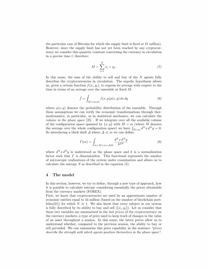
the particular case of Bitcoins for which the supply limit is fixed at 21 million).However, since the supply limit has not yet been reached by any cryptocur-rency we consider this quantity constant concerning the currency in circulationin a precise time t, therefore:
M =
N∑i=1
xi + yi. (7)
In this sense, the sum of the ability to sell and buy of the N agents fullydescribes the cryptocurrencies in circulation. The ergodic hypothesis allowsus, given a certain function f(xi, yi), to express its average with respect to thetime in terms of an average over the ensemble at fixed M :
f =
∫M=const
f(x, y)ρ(x, y) dx dy (8)
where ρ(x, y) denotes the probability distribution of the ensemble. Throughthese assumptions we can verify the economic transformations through ther-modynamics; in particular, as in statistical mechanics, we can calculate thevolume in the phase space [25] . If we integrate over all the available volumeof the configuration space spanned by x, y with M = m (where M denotesthe average over the whole configuration space) we have
∫M=m
dNx dNy = 0.So introducing a thick shell ∆ where ∆ m we can define:
Γ (m) =
∫m<M<m+∆M
dNx dNy
k2N(9)
where dNx dNy is understood as the phase space and k is a normalizationfactor such that Γ is dimensionless. This functional represents the numberof microscopic realizations of the system under examination and allows us tocalculate the entropy S as described in the equation (5).
4 The model
In this section, however, we try to define, through a new type of approach, howit is possible to calculate entropy considering essentially the prices obtainablefrom the currency markets (FOREX).First, we know that cryptocurrencies are used by an approximate number ofeconomic entities equal to 44 million (based on the number of blockchain port-folios[21]) for which N 1. We also know that every subject in our systemis fully described by its ability to buy and sell (xi, yi). Let us consider thatthese two variables are summarized in the last prices of the cryptocurrency onthe currency markets, a type of price used to keep track of changes in the valueof an asset throughout a session. In this sense, the latest prices allow us tounderstand whether, compared to the previous session, the ability to buy orsell prevailed. We can summarize this price capability in the sentence “pricesdescribe the strength with which agents position themselves in the phase space”.
308

The key point is that we can use the function M (described above) because ina certain time t the quantity of cryptocurrencies is constant and quantifiable,in this way we can go back to the previous economic model and determine Γas described in the equation (9). Analytically, we do not consider the numberof economic subjects present in the market but indirectly deduce their “po-sition” in the phase space from the difference between the closing prices. Inparticular, first we cluster the closing price series based on a certain referenceinterval (5 days); as for each cluster there is a maximum and a minimum price,we calculate the difference in terms of necessary steps to pass from one to theother obtaining a certain value of gap G (this assumption is based on theidea that the distance between maximum and minimum is a measure of thedispersion of agents in our phase space); to calculate the “volume” occupiedby the disposition of the agents we use combinatorial analysis, therefore:
Γ = G5 (10)
Once the value of Γ is determined, entropy can be calculated by using theBoltzmann formula:
S = κB ln Γ. (11)
Finally, precisely because Boltzmann’s constant is of the order of Avogadro’snumber, we can “rationalize” this entropy value obtained by multiplying it by1023. Our data analysis shows that in situations where entropy is drasticallyreduced, in the following phase it must grow in an “almost obligatory” way; thisin terms of cryptocurrency prices indicates that in situations in which the gapbetween the maximum and the minimum is drastically reduced in the transitionfrom one cluster to another “almost compulsorily” follows a situation in whichit is certainly wider than the previous one. This type of price-based entropydefines how agents move in the phase space, so it allows us to understand ifthere is more movement towards one area rather than another.
4.1 Dataset
The empirical analysis has been applied to the closing prices of three cryp-tocurrencies, all related to the US dollar (USD), that are:
• Tether, whose price with 4 decimal places requires a step equal to 0.0001;• Bitcoin Cash, whose price with 2 decimal places requires a step equal to
0.01;• Litecoin, whose price with 3 decimal places requires a step equal to 0.001.
Prices are considered with a daily time frame over 1 year, from 1/1/2019 to31/12/2019 and they are clustered in 5 days. To make the figures more clear,the 1-year interval has been divided into 4 trimesters. Furthermore, to bettertest the idea, the same test was carried out also on daily prices at 1 minute of1/4/2020 recorded from 10:56 to 11:52, instead of clustered in 5 minutes. Thedifference from the daily case is that these prices were collected, always fromthe same source, but observed on different currency markets.
Source: Investing.com
309

4.2 Numerical examples
We can start the analysis from the annual case. The first cryptocurrencyanalyzed is Tether (USDT/USD), whose price moves in a neightborhood of 1and consists of 4 decimal places; distinguish the trend of entropy compared toprices in the 4 ranges previously defined.
(a) Closing prices and en-tropy 1/1 - 31/3
(b) Closing prices and en-tropy 1/4 - 29/6
(c) Closing prices and en-tropy 30/6 - 27/9
(d) Closing prices and en-tropy 28/9 - 31/12
Fig. 1: Prices (blue) and entropy (orange) Tether in the period 1/1 - 31/12
As can be seen graphically, when entropy reaches a point of relative mini-mum falling below a certain threshold (it therefore undergoes a sharp reduction)it is forced in the next cluster to grow, almost as if to rebalance itself. In termsof prices, this implies that in the cluster in which the entropy descent occurredthere was a very small gap and, in the subsequent cluster, since entropy in-creases the gap also increases. In this case, the range of variation of prices isvery “narrow” and every movement is important. It is possible, however, to no-tice for example looking at the figure 1 (d) what is the gap value and thereforethe entropy threshold that, if “under”-passed, will cause an immediate growthin the next future.The next cryptocurrency analyzed is Bitcoin Cash (BCH/USD):
310

(a) Closing prices and en-tropy 1/1 - 31/3
(b) Closing prices and en-tropy 1/4 - 29/6
(c) Closing prices and en-tropy 30/6 - 27/9
(d) Closing prices and en-tropy 28/9 - 31/12
Fig. 2: Prices (blue) and entropy (orange) Bitcoin Cash in the period 1/1 -31/12
In this case the figure 2 (d) shows how the gap threshold below which a sharpdrop in entropy occurs can also be quite high (especially in currencies wherehigh volatility allows it to to move many points from one price to another).The last cryptocurrency we have considered is Litecoin (LTC/USD):
311

(a) Closing prices and en-tropy 1/1 - 31/3
(b) Closing prices and en-tropy 1/4 - 29/6
(c) Closing prices and en-tropy 30/6 - 27/9
(d) Closing prices and en-tropy 28/9 - 31/12
Fig. 3: Prices (blue) and entropy (orange) Litecoin in the period 1/1 - 31/12
Also in this cryptocurrency all the situations defined above occur, in par-ticular from the figure 3(d) it can be seen how, following the fact that the first4 clusters are growing despite the gap value being quite low, the gap thresholdto define the drastic descent of entropy is quite low. As for the case of 1-minuteprices, we can summarize the trend of the different cryptocurrencies togetheras shown in figure 4 which shows how all the assumptions made in the previouscase are also respected for prices of this type
312

(a) Tether (b) Bitcoin Cash
(c) Litecoin
Fig. 4: Prices (blue) and entropy (orange) of cryptocurrencies based on 1 minute
In particular, the hypotheses made previously are very evident in the caseof the Tether (figure 4 (a)).
4.3 Possible effects on prediction
Thanks to previous results we can use entropy as an indicator to make pre-dictions on the price trend of cryptocurrencies in the currency markets. Forexample, we can suppose that we are in a certain cluster X where entropy hasdeclined sharply. As previously defined, we expect entropy to grow in the nextcluster and this leads to an increase in the price gap. The hypothesis we canmake is that the value of the gap in the cluster X+1 is at least one unit higherthan the value in the cluster X: we can use this information to understandwhat the future price range will be. In this case, knowing the value of thegap in the cluster X, we can create a bifurcation that represents the possibleevolution of the price in the event of a bullish or bearish trend. Assuming,moreover, that the first cryptocurrency price close enough to the last price ofthe previous cluster what we can expect is such a situation: if the second clos-ing price of the cluster X + 1 is higher than the previous price in the samecluster and assuming an upward trend we can assume that the series of pricescontinues in an area that we have defined as Gap−; while if the second closingprice of the cluster X + 1 is lower than the previous price in the same clusterand assuming a bearish trend we can assume that the price series continues inan area that we have defined as Gap+. Such information can be fundamental
313

for example for an investor who intends to choose the ideal moment to enter(or exit) the market or balance any price limits.
5 Conclusions
In this paper, we have defined a similarity between a thermodynamic systemand a currency system. Thanks to this assumption, we have shown how it’spossible to apply Boltzmann’s entropy to cryptocurrencies. This system ischaracterized by the presence of N subjects interested in buying (or selling) thistype of currency. Assuming that the quantity of money at a certain moment tis fixed and determinable, it is possible to hypothesize that the position of eacheconomic entity is summarized by the last price of the cryptocurrency itself inthe currency markets, as an indicator characterized by the ability to buy andsell. With this hypothesis, it was possible to determine the entropy using theBoltzmann formula, dividing the time interval into clusters and calculating thegap between the different prices. This analysis has shown that when entropyfalls sharply then it must necessarily grow shortly; which in terms of pricecorresponds to a situation in which the gap between maximum and minimumis wider than the previous one.
References
1. Antonopoulos A. A. Mastering Bitcoin: Unlocking Digital Cryptocurrencies.O’Reilly Media, 2014.
2. Dionisio A., Menezes R, and Menezes D. A. An econophysics approach to analyseuncertainty in financial markets: an application to the portuguese stock market.The European Physical Journal, 2006.
3. Renyi A. Probability theory. North-Holland Series in Applied Mathematics andMechanics, 1970.
4. Brissaud J. B. The meanings of entropy. Entropy, 2005.5. BaFin. Merkblatt: Hinweise zum tatbenstand des kryptoverwahrgeschafts. 2020.6. Philippatos G. C. and Wilson C. J. Entropy, market risk and the selection of
efficient portfolios. Applied Economics, 1972.7. Tsallis C. Possible generalization of boltzmann-gibbs statistics. Springer-Verlag,
1988.8. Shannon C. E. and Weaver W. The mathematical theory of communication. Uni-
versity of Illinois Press, 1949.9. Smith E. and Foley D. K. Is utility theory so different from thermodynamics? SFI
Preprint, 2002.10. Usta I. and Kantar Y. M. Mean-variance-skewness-entropy measures: a multi
objective approach for portfolio selection. Entropy, 2011.11. IFRS. Holdings of cryptocurrencies - agenda paper 12. IFRS Staff Paper, 2019.12. Chen J., Duan K., Zhang R., Zeng L., and Wang W. An ai based super nodes
selection algorithm in blockchain networks. arXiv:1808.00216, 2018.13. McCauley J. Thermodynamic analogies in economics and finance: instability of
markets. MPRA, 2004.14. Huang K. Statistical Mechanics. Wiley, 2008.15. Adler R. L., Konheim A. G., and McAndrew M. H. Topological entropy. American
Mathematical Society, 1965.
314

16. Boltzmann L. Vorlesungen uber gastheorie. Leipzig: J. A. Barth., 1896.17. Gulko L. The entropy theory of stock option pricing. Int. J. Theoretical Appl.
Finance, 1999.18. Falcioni M. and Vulpiani A. Meccanica Statistica Elementare. Springer-Verlag,
2015.19. Pincus S. M. Approximate entropy as a measure of system complexity. Proceedings
of the National Academy of Science, 1991.20. Sergeev V. M. Rationality, property rights, and thermodynamic approach to
market equilibrium. Journal of Mathematical Sciences, 2006.21. Szmigiera M. Number of blockchain wallet users globally 2016-2019. Statista,
2020.22. Jana P., Roy T. K., and Mazumder S. K. Multi-objective possibilistic model for
portfolio selection with transaction cost. J. Comput. Appl. Math., 2009.23. Clausius R. Ueber verschiedene fur die anwendung bequeme formen der haupt-
gleichungen der mechanischen warmetheorie. Ann. Phys. Chem., 1865.24. Nakamoto S. Bitcoin: A per-to-peer electronic cash system. Bitcoin.org, 2008.25. Viaggiu S., Lionetto A., Bargigli L., and Longo M. Statistical ensembles for money
and debt. arXiv:1109.0891, 2018.26. Zakiras V., Christopoulos A. G., and Rendoumis V. L. A thermodynamic de-
scription of the time evolution of a stock market index. European Journal ofEconomics, Finance and Administrative Sciences, 2009.
27. Chen W., Wang Z., Xie H., and Yu W. Characterization of surface emg signalbased on fuzzy entropy. IEEE Transaction, 2007.
28. Gibbs J. W. On the equilibrium of heterogeneous substances. Am. J. Sci., 1878.
315

316