Channel Sense

7/31/2019 Channel Sense

http://slidepdf.com/reader/full/channel-sense 1/32

1

Channel Estimation for Opportunistic Spectrum

Access: Uniform and Random Sensing

Quanquan Liang, Mingyan Liu, Member, IEEE,

Abstract

The knowledge of channel statistics can be very helpful in making sound opportunistic spectrum

access decisions. It is therefore desirable to be able to efficiently and accurately estimate channel

statistics. In this paper we study the problem of optimally placing sensing times over a time window so

as to get the best estimate on the parameters of an on-off renewal channel. We are particularly interested

in a sparse sensing regime with a small number of samples relative to the time window size. Using

Fisher information as a measure, we analytically derive the best and worst sensing sequences under a

sparsity condition. We also present a way to derive the best/worst sequences without this condition using

a dynamic programming approach. In both cases the worst turns out to be the uniform sensing sequence,

where sensing times are evenly spaced within the window. With these results we argue that without a

priori knowledge, a robust sensing strategy should be a randomized strategy. We then compare different

random schemes using a family of distributions generated by the circular β ensemble, and propose anadaptive sensing scheme to effectively track time-varying channel parameters. We further discuss the

applicability of compressive sensing for this problem.

Index Terms

Spectrum sensing, channel estimation, Fisher information, random sensing, sparse sensing, uniform

sensing.

Q. Liang and M. Liu are with Department of Electrical Engineering and Computer Science, University of Michigan, Ann

Arbor, MI 48109-2122. Email: [email protected], [email protected]

An earlier version of this paper appeared at the Information Theory and Application Workshop (ITA), UC San Diego, CA,

February 2010.

May 21, 2010 DRAFT



2

I. INTRODUCTION

Recent advances in software defined radio and cognitive radio [1] have given wireless devices

greater ability and opportunity to dynamically access spectrum, thereby potentially significantly

improving spectrum efficiency and user performance [2], [3]. To be able to fully utilize spectrumavailability (either as a secondary user seeking opportunities of idle periods in the presence of

primary users, or as one of many peer users in a multi-user system seeking channels with the

best condition), a key enabling ingredient in dynamic spectrum access is high quality channel

sensing that allows the user to obtain accurate real-time information on the condition of wireless

channels.

Spectrum sensing is often studied in two contexts: at the physical layer and at the MAC layer.

Physical layer spectrum sensing typically focuses on the detection of instantaneous primary user

signals. Several detection methods, such as matched filter detection, energy detection and feature

detection, have been proposed for cognitive radios [4]. MAC layer spectrum sensing [5], [6] is

more of a resource allocation issue, where we are concerned with the scheduling problem of

when to sense the channel and the estimation problem of extracting statistical properties of the

random variation in the channel, assuming that when we decide to sense the physical layer can

provide sufficiently accurate results on instantaneous channel availability. Such channel statistics

can be very helpful in making good channel access decisions, and most studies on opportunistic

spectrum access assume such knowledge.

In this paper we focus on the scheduling of channel sensing and study the effect different

scheduling algorithms have on the accuracy of the resulting estimate we obtain on channel

parameters. In particular, we are interested in the sparse sensing/sampling regime where we can

use only a limited number of measurements over a given period of time. The goal is to decide

how these limited number of measurements should be scheduled so as to minimize the estimation

error within the maximum likelihood (ML) estimator framework. Throughout the paper the terms

sensing and sampling will be used interchangeably.MAC layer channel estimation within the context of cognitive radios has been studied in

recent years. Below we review those most relevant to the present paper. Kim and Shin [5]

introduced a ML estimator for renewal channels using a uniform sampling/sensing scheme where

samples of the channel are taken at regular time intervals. A more accurate, but also much



3

more computationally costly Bayesian estimator was introduced in [8], again based on uniform

sensing. [9] analyzed the relationship between estimation accuracy, number of samples taken

and the channel state transition probabilities by using the sampling and estimation framework

of [5] and focusing on Markovian channels. [10] proposed a Hidden Markov Model (HMM)

based channel status predictor using reinforcement learning techniques. This predictor predicts

next channel state based on past information obtained through uniformly sampling the channel.

[11] presented a channel estimation technique based on wavelet transform followed by filtering.

This method relies on dense sampling of the channel.

In most of the above cited work, the focus is on the estimation problem given (sufficiently

dense) uniform sampling of the channel, i.e., with equal time periods between successive samples.

This scheme will be referred to as uniform sensing in the remainder of this paper. By contrast,

sampling schemes where time intervals between successive samples are drawn from a certain

probability distribution will be referred to as random sensing throughout the paper. We observe

that due to constraints on time, energy, memory and other resources, a user may wish to perform

channel sensing at much lower frequencies while still hoping for good estimates. This could be

relevant for instance in cases where a user wants to track the channel condition in between active

data communication, or where a user needs to track a large number of different channels. It is

this sparse sampling scenario that we will focus on in this study, and the goal is to judiciously

schedule these limited number of samples.

Our main contributions are summarized as follows.

• We demonstrate that when sampling is done sparsely, random sensing significantly outper-

forms uniform sensing.

• In the special case of exponentially distributed on/off durations, we derive tight lower and

upper bounds on the Fisher information under a sparsity condition, while obtaining the best

and worst possible sampling schemes measured by the Fisher information. We show that

uniform sensing is the worst one can do; any deviation from it improves the estimation

accuracy.

• We present a dynamic programming approach to obtain the best and worst sampling se-

quences in the more general case without the sparsity condition.

• We show that under the same channel statistics and the same average sampling interval (or

frequency), a random sensing scheme affects the estimation accuracy through the higher-



4

order central moments of the sampling intervals, and use the circular β ensemble to study

a family of distributions.

• We present an adaptive random sensing scheme that can very effectively track time-varying

channel parameters, and is shown to outperform its counterpart using uniform sensing.

The remainder of this paper is organized as follows: Section II presents the channel models and

Section III gives the detail of the ML estimator. Then in Section IV we present how the sampling

scheme affects the estimation performance; the best and worst sensing sequences with and

without a sparse sampling condition are obtained. In Section V we use a family of distributions

generated by the circular β ensemble to examine different random sampling schemes. Section

VI presents an adaptive random sensing scheme, and Section VII discusses the applicability of

compressive sensing in this problem. Section VIII concludes the paper.

II. THE CHANNEL MODEL

In this paper we will limit our attention to MAC layer spectrum sensing as mentioned in the

introduction. Within this context, the channel state perceived by a secondary user is represented

by a binary random variable. This is a model commonly used in a large volume of literature,

from channel estimation (e.g., [5], [9]) to opportunistic spectrum access (e.g., [6]) to spectrum

measurement (e.g., [12]). Specifically, let Z (t) denote the state of the channel at time t, such

that

Z (t) = 1 if the channel is sensed busy at time t ,

Z (t) = 0 otherwise .

The advantage of such a model is its simplicity and tractability in many instances. The

weakness lies in the fact that the actual energy present or detected in the channel is hardly

binary. The raw channel measurement data will have to go through a binary hypothesis test

(e.g., via thresholding) to be reduced to the above form, a process that comes with probabilities

of error. Consequently, the channel is sensed to be in either state with a detection probability

and a false alarm probability.

In this paper our focus is on extracting and estimating essential statistics given a sequence of

measured channel states (0s and 1s) rather than the binary detection of channel state (deciding

between 0 and 1 given the energy reading). For this purpose, we will assume that the channel

state measurements are error-free. If we have side information on what the detection and false



5

alarm probabilities are, then the estimation results may be adjusted accordingly to utilize such

knowledge.

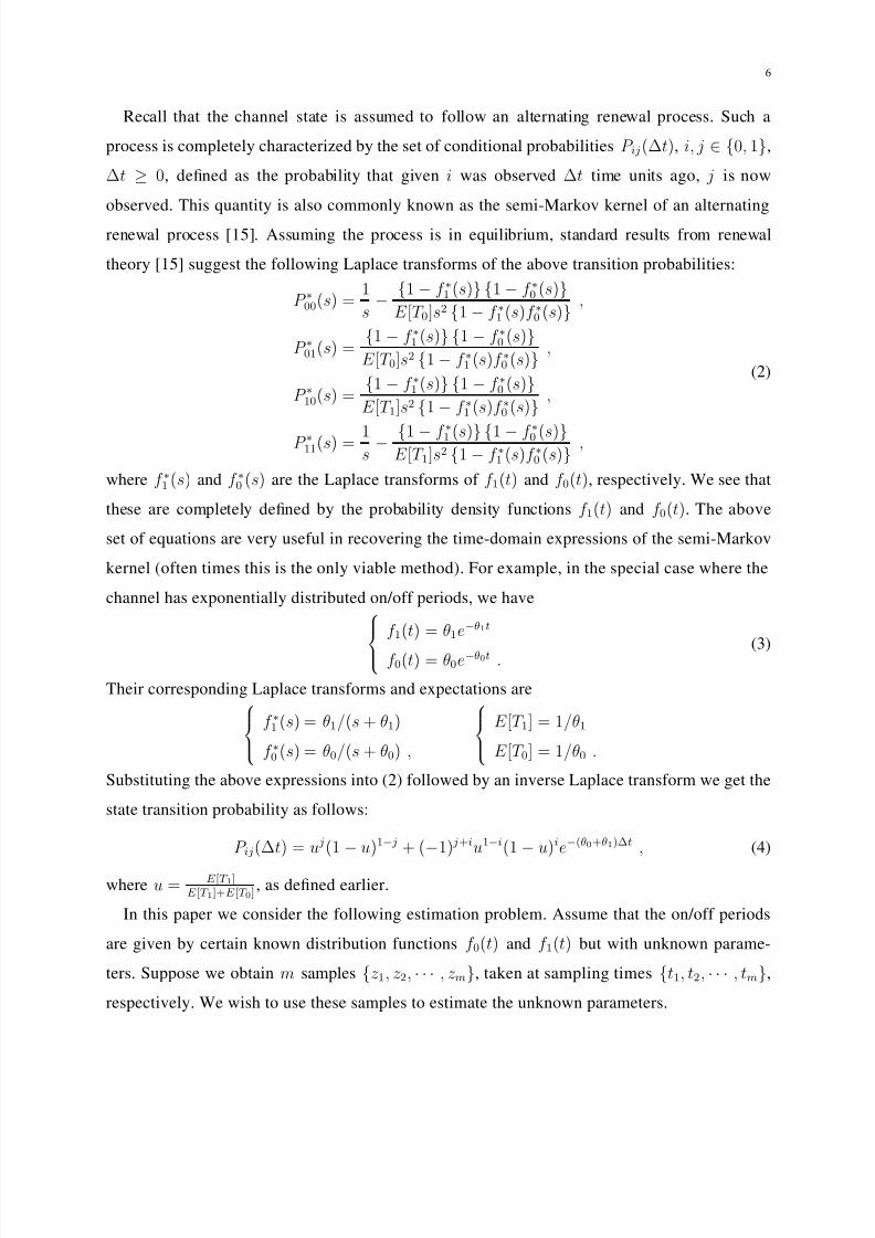
The channel state process Z (t) is assumed to be a continuous-time alternating renewal process,

alternating between on/busy (state “1”) and off/idle (state “0”), an illustration is given in Figure

1. Typically, it is assumed that a secondary user can utilize the channel only when it is sensed

to be in the off states (i.e., when the channel is idle or the primary user is absent). When the

channel state transitions to the on state, the secondary user is required to vacate the channel so

as not to interfere with the primary user (also referred to as the spectrum underlay paradigm,

see e.g., [13]).

This random process is completely defined by two probability density functions f 1(t) and

f 0(t), t > 0, i.e., the probability distribution of the sojourn times of the on periods (denoted by

the random variable T 1) and the off periods (denoted by the random variable T 0), respectively.

The channel utilization u is defined as

u =E [T 1]

E [T 1] + E [T 0], (1)

which is also the average fraction of time the channel is occupied or busy. By the definition

of a renewal process, T 1 and T 0 are independent and all on (off) periods are independently and

identically distributed. It’s worth pointing out that the widely used Gilbert-Elliot model (a two-

state Markov chain) is a special case of the alternating renewal process where the on (off) periods

are exponentially (in the case of continuous time) or geometrically (in the case of discrete time)

distributed.

Fig. 1. Channel model: alternating renewal process with on and off states

III. MAXIMUM LIKELIHOOD (ML) BASED CHANNEL ESTIMATION

We proceed to describe the maximum likelihood (ML) estimator [14] we will use to estimate

channel parameters from a sequence of channel state observations.



6

Recall that the channel state is assumed to follow an alternating renewal process. Such a

process is completely characterized by the set of conditional probabilities P ij(∆t), i, j ∈ {0, 1},

∆t ≥ 0, defined as the probability that given i was observed ∆t time units ago, j is now

observed. This quantity is also commonly known as the semi-Markov kernel of an alternating

renewal process [15]. Assuming the process is in equilibrium, standard results from renewal

theory [15] suggest the following Laplace transforms of the above transition probabilities:

P ∗00(s) =1

s− {1 − f ∗1 (s)} {1 − f ∗0 (s)}

E [T 0]s2 {1 − f ∗1 (s)f ∗0 (s)} ,

P ∗01(s) ={1 − f ∗1 (s)} {1 − f ∗0 (s)}

E [T 0]s2 {1 − f ∗1 (s)f ∗0 (s)} ,

P ∗10(s) ={1 − f ∗1 (s)} {1 − f ∗0 (s)}

E [T 1]s2 {1 − f ∗1 (s)f ∗0 (s)} ,

P ∗11(s) = 1s

− {1 − f ∗1 (s)} {1 − f

∗0 (s)}

E [T 1]s2 {1 − f ∗1 (s)f ∗0 (s)} ,

(2)

where f ∗1 (s) and f ∗0 (s) are the Laplace transforms of f 1(t) and f 0(t), respectively. We see that

these are completely defined by the probability density functions f 1(t) and f 0(t). The above

set of equations are very useful in recovering the time-domain expressions of the semi-Markov

kernel (often times this is the only viable method). For example, in the special case where the

channel has exponentially distributed on/off periods, we have

f 1(t) = θ1e−θ1t

f 0(t) = θ0e−θ0t . (3)

Their corresponding Laplace transforms and expectations are

f ∗1 (s) = θ1/(s + θ1)

f ∗0 (s) = θ0/(s + θ0) ,

E [T 1] = 1/θ1

E [T 0] = 1/θ0 .

Substituting the above expressions into (2) followed by an inverse Laplace transform we get the

state transition probability as follows:

P ij(∆t) = u j(1

−u)1− j + (

−1) j+iu1−i(1

−u)ie−(θ0+θ1)∆t , (4)

where u = E [T 1]E [T 1]+E [T 0]

, as defined earlier.

In this paper we consider the following estimation problem. Assume that the on/off periods

are given by certain known distribution functions f 0(t) and f 1(t) but with unknown parame-

ters. Suppose we obtain m samples {z1, z2, · · · , zm}, taken at sampling times {t1, t2, · · · , tm},

respectively. We wish to use these samples to estimate the unknown parameters.



7

First note that the channel utilization factor u can be estimated through the sample mean of

the m measurements as follows

u =1

m

mi=1

zi . (5)

Let θ be the unknown parameters of the on/off distributions: θ = {θ1, θ0}. Note that in general

θ1 and θ0 are vectors themselves. Then the likelihood function is given by

L(θ) = P r{Z ; θ}

= P r{Z tm = zm, Z tm−1 = zm−1, Z tm−2 = zm−2, . . . , Z t1 = z1; θ} . (6)

The idea of ML estimation is to find the value of θ that maximizes the log likelihood function

ln L(θ), i.e., the estimate θ is such that∂ lnL(θ)

∂θ|ˆθ

= 0. This method has been used extensively

in the literature [16]–[20]. For a fixed set of data and underlying probability model, the ML

estimator selects the parameter value that makes the data “most likely” among all possible

choices. Under certain (fairly weak) regularity conditions the ML estimator is asymptotically

optimal [21].

The question we wish to investigate is what impact the selection of the sampling time sequence

{t1, t2, · · · , tm} has on the performance of this estimator, given a limited number of samples m.

Specifically, we question whether random sampling is a better way of sensing the channel than

uniform sampling where the measurement samples are taken at regular time intervals.

For the remainder of our analysis we will limit our attention to the case where the channel

on/off durations are given by exponential distributions. This is for both mathematical tractability

and simplicity of presentation. We explore other distributions in our numerical experiments.

Since the exponential distribution is defined by a single parameter, we have now θ = {θ1, θ0},

where θ1 and θ0 are the two unknown scalar parameters of the on and off exponential distributions,

respectively. Using the memoryless property, the likelihood function becomes

L(θ) = P r{Z ; θ}

= P r{Z t1 = z1; θ} ·mi=2

P r{Z ti = zi|Z ti−1 = zi−1; θ}

= P r{Z t1 = z1; θ} ·mi=2

P zi−1zi(∆ti; θ) . (7)

where ∆ti = ti − ti−1. The first quantity on the right is taken to be

P r{zt1 = z1; θ} = uz1(1 − u)1−z1 . (8)



8

That is, the probability of finding the channel in a particular state (LHS of Eqn (8)) is taken to

be the stationary distribution given by the RHS. This choice is justified by assuming that the

channel is in equilibrium.

The second quantity P zi−1zi(∆ti; θ) is given in Eqn (4). Combining these two quantities, we

have

L(θ0, θ1) =L(θ)

=uz1(1 − u)1−z1mi=2

uzi(1 − u)1−zi + (−1)zi+zi−1u1−zi−1(1 − u)zi−1e−(θ0+θ1)∆ti

.

(9)

The estimates for the parameters are found by solving

∂ lnL(θ0,θ1)

∂θ0= 0

∂ lnL(θ0,θ1)∂θ1

= 0 . (10)

Technically, to get the estimates for both θ0 and θ1 one needs to solve the above two equations

simultaneously. This however proves to be computationally complex and analytically intractable.

Instead, we adopt the following estimation procedure. We first estimate u using Eqn (5), and

take θ1 = (1−u)θ0u

. Due to the exponential assumption, it can be shown that this estimate of

u is unbiased regardless of the sequence {t1, · · · , tm} as long as it is determined offline. The

likelihood function (9) can then be re-written as

L(θ0) =uz1(1 − u)1−z1mi=2

uzi(1 − u)1−zi + (−1)zi+zi−1u1−zi−1(1 − u)zi−1e−θ0∆ti/u

. (11)

The estimation of θ0 is then derived by solving the equation∂ lnL(θ0)

∂θ0= 0.

In our analysis, we will use this procedure by treating u as a known constant and solely focus

on the estimation of θ0, with the understanding that u is separately and unbiasedly estimated,

and once we have the estimate for θ0 we have the estimate for θ1. It has to be noted that this

procedure is in general not equivalent to solving (10) simultaneously. However, we have found

this to be a very good approximation, computationally feasible, and much more amenable to

analysis.

IV. BEST AND WORST SAMPLING SEQUENCES

The goal of this study is to judiciously schedule a very limited number of sampling times so

that the estimation accuracy is least affected. We first argue intuitively why the commonly used



9

uniform sampling does not perform well when the number of samples allowed is limited. This

motivates us to look for better sampling schemes. We then present a precise analysis through

the use of Fisher information, in the case of exponential on/off distributions. In particular, we

will show that using this measure, under a certain sparsity condition, uniform sensing is the

worst schedule in terms of its estimation accuracy. We also derive an upper bound on the Fisher

information as well as the sampling sequence achieving this upper bound. These provide us

with useful benchmarks to assess any arbitrary sampling sequence. We then present a dynamic

programming approach to finding the best and worst sampling sequence without the sparsity

condition, which provides a further bound on how well any sampling sequence can be expected

to perform.

A. An intuitive explanation

Uniform sensing, where samples are taken at constant time intervals, is a natural, easy-to-

implement, and easy-to-analyze scheme. Specifically, with the on/off durations being exponential

the likelihood function has a particularly simple form; there is also a closed-form solution to

the maximization of the log likelihood function, see e.g., [5]. However, when sensing is done

sparsely, certain problems arise. One of the first things to note is that since there is no variation

across sampling intervals under uniform sensing, the uniform interval in general needs to be

upper-bounded in order to catch potential channel state changes that occur over small intervals1

.This bound cannot be guaranteed under sparse sensing. If sensing is done randomly, then even if

the average sampling interval is large, there can be significant probability for sufficiently small

sampling intervals to exist in any realization of the sampling time sequence {t1, t2, · · · , tm}.

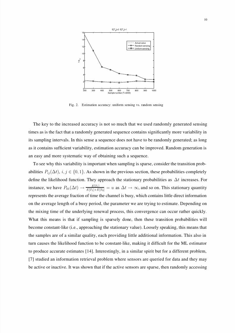
We show in Figure 2 a comparison between uniform sensing and random sensing where the

sensing times are randomly placed using a uniform distribution 2 within a window of 5000 time

units. The on/off periods are exponentially distributed with parameters E [T 0] = 2, E [T 1] = 1

time units, respectively. The figure shows the estimated value of E [T 0] as a function of the

number of samples taken within the window of 5000. We see that random sensing outperforms

uniform sensing, and significantly so when m is small.

1One such upper bound was proposed in [5].

2Here uniform distribution refers to the sampling times being randomly placed within the window following a uniform

distribution, not to be confused with uniform sensing where sampling intervals are a constant.



10

200 300 400 500 600 700 800 900 10000

2

4

6

8

10

12

14

16

Sample number (T=5000)

1 / θ

0

E[T0]=2 E[T

1]=1

Actual value

Random sensing

Uniform sensing

Fig. 2. Estimation accuracy: uniform sensing vs. random sensing

The key to the increased accuracy is not so much that we used randomly generated sensing

times as is the fact that a randomly generated sequence contains significantly more variability in

its sampling intervals. In this sense a sequence does not have to be randomly generated; as long

as it contains sufficient variability, estimation accuracy can be improved. Random generation is

an easy and more systematic way of obtaining such a sequence.

To see why this variability is important when sampling is sparse, consider the transition prob-

abilities P ij(∆t), i, j∈ {

0, 1}

. As shown in the previous section, these probabilities completely

define the likelihood function. They approach the stationary probabilities as ∆t increases. For

instance, we have P 01(∆t) → E [T 1]E [T 1]+E [T 0]

= u as ∆t → ∞, and so on. This stationary quantity

represents the average fraction of time the channel is busy, which contains little direct information

on the average length of a busy period, the parameter we are trying to estimate. Depending on

the mixing time of the underlying renewal process, this convergence can occur rather quickly.

What this means is that if sampling is sparsely done, then these transition probabilities will

become constant-like (i.e., approaching the stationary value). Loosely speaking, this means that

the samples are of a similar quality, each providing little additional information. This also in

turn causes the likelihood function to be constant-like, making it difficult for the ML estimator

to produce accurate estimates [14]. Interestingly, in a similar spirit but for a different problem,

[7] studied an information retrieval problem where sensors are queried for data and they may

be active or inactive. It was shown that if the active sensors are sparse, then randomly accessing



11

them outperforms periodic (or uniform) schedules.

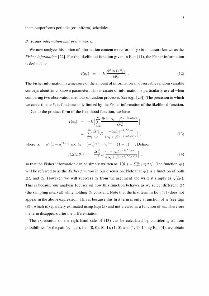
B. Fisher information and preliminaries

We now analyze this notion of information content more formally via a measure known as the

Fisher information [22]. For the likelihood function given in Eqn (11), the Fisher information

is defined as:

I (θ0) = −E [∂ 2 ln L(θ0)

∂θ20

] . (12)

The Fisher information is a measure of the amount of information an observable random variable

conveys about an unknown parameter. This measure of information is particularly useful when

comparing two observation methods of random processes (see e.g., [23]). The precision to which

we can estimate θ0 is fundamentally limited by the Fisher information of the likelihood function.

Due to the product form of the likelihood function, we have

I (θ0) = −E mi=2

∂ 2 ln[αi + β ie−θ0∆ti/u]

∂θ20

=mi=2

∆t2iu2

E −αiβ ie

−θ0∆ti/u

(αi + β ie−θ0∆ti/u)2

, (13)

where αi = uzi(1 − u)1−zi and β i = (−1)zi+zi−1u1−zi−1(1 − u)zi−1. Define:

g(∆ti; θ0) =

∆t2iu2 E

−αiβ ie

−θ0∆ti/u

(αi + β ie−θ0∆ti/u)2

, (14)

so that the Fisher information can be simply written as I (θ0) =m

i=2 g(∆ti). The function g()

will be referred to as the Fisher function in our discussion. Note that g() is a function of both

∆ti and θ0. However, we will suppress θ0 from the argument and write it simply as g(∆t).

This is because our analysis focuses on how this function behaves as we select different ∆t

(the sampling interval) while holding θ0 constant. Note that the first term in Eqn (11) does not

appear in the above expression. This is because this first term is only a function of u (see Eqn

(8)), which is separately estimated using Eqn (5) and not viewed as a function of θ0. Thereforethe term disappears after the differentiation.

The expectation on the right-hand side of (13) can be calculated by considering all four

possibilities for the pair (zi−1, zi), i.e., (0, 0), (0, 1), (1, 0), and (1, 1). Using Eqn (4), we obtain



12

the transition probability of each case to be (1 − u)P 00(∆t), (1 − u)P 01(∆t), uP 10(∆t) and

uP 11(∆t), respectively. We can therefore calculate the Fisher function as follows:

g(∆t) =∆t2

u2e−θ0∆t/u

u2(1 − u)

u

−ue−θ0∆t/u

+u(1 − u)2

(1

−u)

−(1

−u)e−θ0∆t/u

− u(1 − u)2

(1 − u) + ue−θ0∆t/u− u2(1 − u)

u + (1 − u)e−θ0∆t/u

. (15)

Below we show that under a certain sparsity condition on the sampling rate, the Fisher function

is strictly convex, and that the Fisher information is minimized when uniform sampling is used.

We begin by introducing this sparsity condition.

Condition 1: (Sparsity condition) Let α = max{2 +√

2, ln(1−uu ), ln( u1−u

)}. This condition

requires that ∆t > αu/θ0.

Taking ∆t to be the time between two consecutive sampling points, the above condition states

that these two points cannot be too close together with respect to the average off duration (1/θ0)

and the channel utilization u.

Lemma 1: The Fisher function g(∆t) given in Eqn (15) is strictly convex under Condition 1

(i.e, for ∆t > αu/θ0).

The proof of this lemma can be found in the Appendix. Using this lemma we next derive

tight lower and upper bounds of the Fisher information.

C. A tight lower bound on the Fisher information

Lemma 2: For any n ∈ N, n ≥ 1, T ∈ R, T > (n + 1)αu/θ0, and αu/θ0 < ∆t < T −nαu/θ0,

the function G(∆t) = ng(T −∆tn ) + g(∆t) has a minimum of (n + 1)g( T

n+1) attained at ∆t = T n+1

.

Proof: Setting the first derivative of G to zero and solving for ∆t results in solving the

equation g′

(∆t) = g′

(T −∆tn

). Since the arguments on both side satisfy Condition 1, by the

assumption of the lemma, g is strictly convex according to Lemma 1 and g′

is a strictly monotonic

function. Therefore there exists a unique solution within the range of (αu/θ0, T − nαu/θ0) to

this equation at ∆t = T

n+1

.

Next we calculate the second derivative of G at this point. Since G′′

(∆t) = g′′

(∆t) +

1ng

′′

(T −∆tn ), we have G

′′

( T n+1) = (1 + 1

n)g′′

( T n+1). Since T > (n + 1)αu/θ0, g is convex at this

stationary point by Lemma 1. Hence G is convex at this point and it is thus a global minimum

within the range (αu/θ0, T − nαu/θ0); the minimum value is (n + 1)g( T n+1), completing the

proof.



13

Theorem 1: Consider a period of time [0, T ], in which we wish to schedule m ≥ 3 sampling

points, including one at time 0 and one at time T . Denote the sequence of time spacings between

these samples as ∆t = [∆t2, ∆t3, · · · , ∆tm], wherem

i=2 ∆ti = T . For a given sequence ∆t,

define the Fisher information I (θ0) as in Eqn (13) and rewrite it as I (θ0; ∆t) to emphasize its

dependence on ∆t. Assuming T > (m − 1)αu/θ0, then we have

min∆t∈Am

I (θ0; ∆t) = (m − 1)g(T

m − 1),

where Am = {∆ti :m

i=2 ∆ti = T, ∆ti > αu/θ0, i = 2, · · · , m}, and with the minimum

achieved at ∆ti = T m−1 , i = 2, · · · , m.

Proof: We prove this by induction on m.

Induction basis: For m = 3,

I (θ0; ∆t) = g(∆t2) + g(∆t3).

Using Lemma 1 in the special case of n = 1 the result follows.

Induction step: Suppose the result holds for 3, 4, . . . m, we want to show it also holds for

m + 1 for T > mαu/θ0. Note that in this case ∆t ∈ Am+1 implies that αu/θ0 < ∆tm+1 <

T − (m − 1)αu/θ0, which will be denoted as ∆tm+1 ∈ Am+1 below for convenience. We thus

have

min∆t∈Am+1{I (θ0; ∆t)}= min

∆t∈Am+1

mi=2

g(∆ti) + g(∆tm+1)

= min∆tm+1∈Am+1

min

∆ti=T −∆tm+1

mi=2

g(∆ti)

+ g(∆tm+1)

= min∆tm+1∈Am+1

(m − 1)g(

T − ∆tm+1

m − 1) + g(∆tm+1)

= mg(T

m) ,

where the third equality is due to the induction hypothesis and the first term on the RHS is

obtained at ∆ti = T −∆tm+1

m−1 , i = 2, . . . , m. The last equality invokes Lemma 2 in the special case

of n = m − 1, and is obtained at ∆tm+1 = T m

. Combining these we conclude that the minimum

value of Fisher information is mg( T m), when ∆ti = T

m , i = 2, . . . , m + 1. Thus the case m + 1

also holds, completing the proof.



14

Theorem 1 states that given the total sensing period T and the total number of samples m,

provided that the sampling is done sparsely (with sufficiently large sampling intervals as defined

in Condition 1), the Fisher information attains its minimum when all sampling intervals have

the same value, i.e when using a uniform sensing schedule. In this sense uniform sensing is the

worst possible sensing scheme; any deviation from it, while keeping the same average sampling

interval T /(m − 1), can only increase the Fisher information. As we have seen in Figure 2, this

increase in Fisher information becomes more significant when sampling gets sparser, i.e., when

m decreases.

D. A tight upper bound on the Fisher information

The derivation of the upper bound follows very similar steps as those for the lower bound.

Lemma 3: For any T ∈ R, T > 2αu/θ0, and αu/θ0 < ∆t < T − αu/θ0, the function

F (∆t) = g(T −∆t)+ g(∆t) has a maximum of g(αu/θ0)+ g(T −αu/θ0) attained at ∆t = αu/θ0

or ∆t = T − αu/θ0.

Proof: Firstly we prove that F is convex under the stated conditions. We have

F ′

(∆t) = g′

(∆t) − g′

(T − ∆t) .

Since g is strictly convex under the stated conditions, by Lemma 1 g′

is monotonic increasing.

Thus F ′

is also monotonic increasing, hence F is convex. It follows that the maximum of F (∆t)

is attained at one and/or the other extreme point of ∆t. In either case we have

F (αu/θ0) = F (T − αu/θ0) = g(αu/θ0) + g(T − αu/θ0).

Theorem 2: Consider a period of time [0, T ], in which we wish to schedule m ≥ 3 sampling

points, including one at time 0 and one at time T . Denote the sequence of time spacings between

these samples as ∆t = [∆t2, ∆t3, · · · , ∆tm], where

mi=2 ∆ti = T . Assuming T > (m−1)αu/θ0,

then we have

max∆t∈Am

I (θ0; ∆t) = (m − 2)g(αu/θ0) + g(T − (m − 2)αu/θ0),

where Am = {∆ti :m

i=2 ∆ti = T, ∆ti > αu/θ0, i = 2, · · · , m}, and with the maximum

achieved at ∆ti = αu/θ0, i = 2, · · · , m − 1 and ∆tm = T − (m − 2)αu/θ0.

Proof: We prove this by induction on m.



15

Induction basis: For m = 3, I (θ0; ∆t) = g(∆t2) + g(∆t3). Using Lemma 3 the result

immediately follows.

Induction step: Suppose the result holds for 3, 4, . . . m, we want to show it also holds for

m + 1 for T > mαu/θ0. Again in this case ∆t∈ A

m+1 implies that αu/θ0 < ∆tm+1 <

T − (m − 1)αu/θ0, which will be denoted as ∆tm+1 ∈ Am+1 for convenience. We thus have

max∆t∈Am+1

{I (θ0; ∆t)}

= max∆t∈Am+1

mi=2

g(∆ti) + g(∆tm+1)

= max∆tm+1∈Am+1

max

∆ti=T −∆tm+1

mi=2

g(∆ti)

+ g(∆tm+1)

= max∆tm+1∈Am+1

(m − 2)g(αu/θ0) + g(T − ∆tm+1 − (m − 2)αu/θ0) + g(∆tm+1)

= (m − 1)g(αu/θ0) + g(T − (m − 1)αu/θ0) ,

where the third equality is due to the induction hypothesis and the first term on the RHS is

obtained at ∆ti = αu/θ0, i = 2, . . . , m − 1 and ∆tm = T − ∆tm+1 − (m − 2)αu/θ0. The last

equality invokes Lemma 3, and is obtained at ∆tm+1 = T − (m − 1)αu/θ0 or ∆tm+1 = αu/θ0.

Thus the case m + 1 also holds, completing the proof.

We see from this theorem that under the sparsity condition, the best sensing sequence is to

sample at the smallest interval that the condition would allow, till we use all the m − 2 samples

we have the freedom of placing. This produces a uniform sequence of sampling times except

for the last one. It can be shown that if we remove the constraint of having a window of T ,

but rather seek to optimally place m points subject to the sparsity condition, then the optimal

sequence would be exactly uniform with the interval ∆ti = αu/θ0. However, since θ0 is the very

thing we are trying to estimate, it would be unreasonable to suggest that this optimal interval is

known a priori. Therefore, this optimal sequence, while exists, is not in general implementable.

E. Best and worst sampling schemes without the sparsity condition

The preceding upper- and lower-bound achieving sensing sequences were derived under the

sparsity Condition 1. Below we show how to obtain the best and worst sensing sequences in a

more general setting, without the requirement of Condition 1, via the use of dynamic program-

ming. While this result is more general compared to those derived under the sparsity condition,



16

structurally they are not as easy to identify and are thus given in a numerical form. These

sequences are also not practically implementable as they also assume the a priori knowledge of

the parameters to be estimated.

Denote by π a sampling policy given by the time sequence

{t1, t1,

· · ·, tm

}. Then the optimal

sampling policy is given by

π∗ = arg maxπ∈Π

I (θ0) , (16)

where the set of admissible policies Π = {ti : t1 = 0, tm = T, 0 < t2 < · · · < tm−1 < T }.

The maximum I (θ0) can be recursively solved through the set of dynamic programming

equations given below:

V (1, t) = g(T

−t),

∀0

≤t < T ;

V (k, t) = maxt<x<T

[g(x − t) + V (k − 1, x)], ∀ 0 ≤ t < T, k = 2, 3, · · · , m − 1 , (17)

and

max I (θ0) = max0<t<T

[g(t) + V (m − 1, t)] . (18)

Here the value function V (k, t) denotes the maximum achievable Fisher information given we

last sampled at time t, with k points remaining to be placed between (t, T ].

Note that since t is continuous, the pair (k, t) has an uncountable state space. In computing

the DP equation (17) we discretize t and T into small steps and require that both be integer

multiples of this small quantity. The resulting DP has a finite state space and can be solved

backwards in time in a standard manner.

It is straightforward to see the exact same procedure can be used to find the sampling sequence

that minimizes the Fisher information, thus giving the worst sampling sequence. It turns out that

the worst sampling sequence in this case coincides with the worst sequence derived under the

sparsity condition, i.e., it is also the uniform sequence.

F. A comparison

We now compare the different sensing sequences we obtained in this section using an example.

They are illustrated in Figure 3(a). In this example the channel parameters are E [T 0] = 5 and

E [T 1] = 3 time units, respectively. The time window is set to be 40 time units, and the channel can



17

only be sensed 5 times. Shown in the figure are the uniform sensing sequence, the best/worst

sensing sequences derived under the sparsity condition, and the best/worst sequences derived

using dynamic programming. As mentioned earlier, the worst obtained via dynamic programming

coincides with the uniform sampling sequence. The worst under the sparsity condition also

coincides with the uniform sequence, a fact proven in Theorem 1, as the sparsity condition

holds in this case. In Figure 3(b), we compared the performance of these sampling strategies, by

setting the time window to 5000 time units. The estimated value under each strategy is shown as

a function of the number of samples taken. The true value is also shown for comparison. These

are used as benchmarks in the next section in evaluating random sensing schemes.

(a) Illustration of different sampling sequences

10 20 30 40 50 60 70 80 900

5

10

15

20

25

30

35


1 / θ 0

E[T0]=5 E[T

1]=3

Actual value

Best by DPUniform/worst by DP/worst under sparsity condition

Best under sparsity condition

(b) Performance comparison

Fig. 3. Comparison of different sampling sequence

As we can see from Figure 3(a), the best sensing sequence produced by dynamic programming

without the sparsity condition also appears to be uniform except for the last sample, as is the

case with the best sequence under the sparsity condition 3. The difference is that the former uses

a smaller interval value that violates the sparsity condition. As mentioned earlier, if we were

to remove the requirement that one sample be placed at time T , then the optimal sequence of

m would appear to be uniform (again, this conclusion is drawn empirically in the case of no

sparsity requirement, and precisely and analytically in the case of sparsity), with the optimal

3Note however that this conclusion is drawn empirically from a large amount of numerical experiment in the case of not

requiring sparsity. By contrast, under the sparsity condition the conclusion is drawn analytically in Theorem 2.



18

interval being the value that maximizes (15). Interestingly, the worst sequence is also uniform

with or without the sparsity condition.

What this result suggests is that in the ideal case if we have a priori knowledge of the channel

parameters, to maximize the Fisher information the best thing to do is indeed to sense uniformly.

The difficulty of course is that without this knowledge we have no way of deciding what the

optimal interval should be, and uniform sensing would be a bad decision as it could turn out to

be the worst with an unfortunate choice of the sampling interval.

In such cases, the robust thing to do is simply to sense randomly, so that with some probability

we will have sampling intervals close to the actual optimum. This is investigated in the next

section.

V. RANDOM SENSING

Under a random sensing scheme, the sampling intervals ∆ti are generated according to some

distribution f (∆t) (this may be done independently or jointly). Below we first analyze how the

resulting Fisher information is affected, and then use a family of distributions generated by the

circular β ensemble to examine the performance of different distributions.

A. Effect on the Fisher information

We begin by examining the expectation of the Fisher function, averaged over randomlygenerated sampling intervals, calculated as follows:

E [g(∆t)] = ∞0

g(∆t)f (∆t)d∆t (19)

= ∞0

[g(µo) + g′(µo)(∆t − µo)

+ · · · +g(n)(µo)(∆t − µo)n

n!+ · · · ]f (∆t)d∆t

= g(µo) + g′(µo)µ1 + · · · +g(n)(µo)µn

n!+ · · ·

where the Taylor expansion is around the expected sampling interval µo = E [∆t], or T /(m − 1)

for given window T and m number of samples taken, and µn = ∞0 (∆t − µo)nf (∆t)d∆t is the

nth order central moment of ∆t.

In order to have a fair comparison we will assume T and m are fixed, thus fixing the average

sampling interval µo under different sampling schemes. Also note that the value g(n)(µo) is



19

completely determined by the channel statistics and not the sampling sequence. Consequently

the expected value of the Fisher function is affected by the selection of a sampling scheme only

through the higher order central moments of the distribution f (). Note that the expectation of

the Fisher function under uniform sampling with constant sampling interval µo is simply g(µo)

(i.e., only the first term on the right hand side remains). Therefore any random scheme would

improve upon this if it results in a positive sum over the higher order terms. While the above

equation does not immediately lead to an optimal selection of a random scheme, it is possible to

seek one from a family of distribution functions through optimization over common parameters.

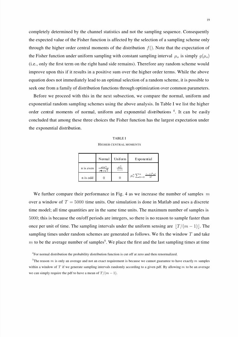
Before we proceed with this in the next subsection, we compare the normal, uniform and

exponential random sampling schemes using the above analysis. In Table I we list the higher

order central moments of normal, uniform and exponential distributions 4. It can be easily

concluded that among these three choices the Fisher function has the largest expectation under

the exponential distribution.

TABLE I

HIGHER CENTRAL MOMENTS

Normal Uniform Exponential

n is even n!σn

(n2)!2

n2

µno

n+1

n is odd 0 0 µ

n

on

k=0

(−1)kn!

k!

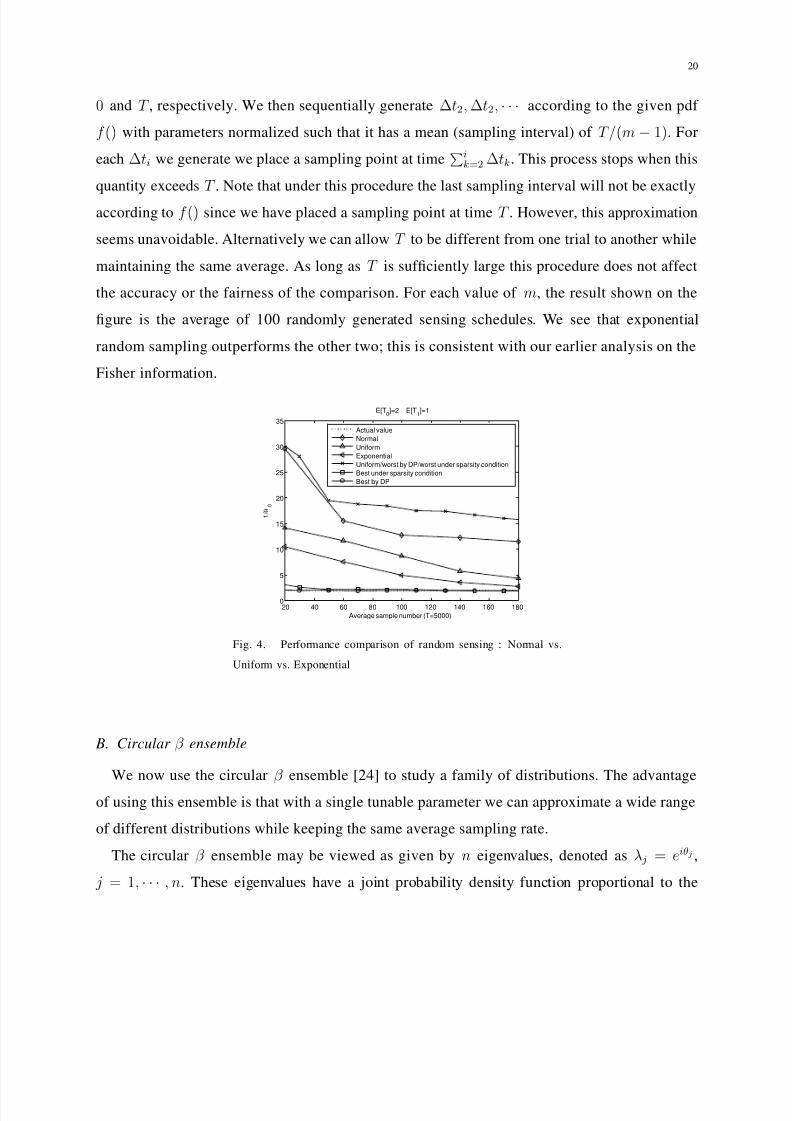
We further compare their performance in Fig. 4 as we increase the number of samples m

over a window of T = 5000 time units. Our simulation is done in Matlab and uses a discrete

time model; all time quantities are in the same time units. The maximum number of samples is

5000; this is because the on/off periods are integers, so there is no reason to sample faster than

once per unit of time. The sampling intervals under the uniform sensing are ⌊T /(m − 1)⌋. The

sampling times under random schemes are generated as follows. We fix the window T and takem to be the average number of samples5. We place the first and the last sampling times at time

4For normal distribution the probability distribution function is cut off at zero and then renormalized.

5The reason m is only an average and not an exact requirement is because we cannot guarantee to have exactly m samples

within a window of T if we generate sampling intervals randomly according to a given pdf. By allowing m to be an average

we can simply require the pdf to have a mean of T/(m− 1).



20

0 and T , respectively. We then sequentially generate ∆t2, ∆t2, · · · according to the given pdf

f () with parameters normalized such that it has a mean (sampling interval) of T /(m − 1). For

each ∆ti we generate we place a sampling point at timei

k=2 ∆tk. This process stops when this

quantity exceeds T . Note that under this procedure the last sampling interval will not be exactly

according to f () since we have placed a sampling point at time T . However, this approximation

seems unavoidable. Alternatively we can allow T to be different from one trial to another while

maintaining the same average. As long as T is sufficiently large this procedure does not affect

the accuracy or the fairness of the comparison. For each value of m, the result shown on the

figure is the average of 100 randomly generated sensing schedules. We see that exponential

random sampling outperforms the other two; this is consistent with our earlier analysis on the

Fisher information.

20 40 60 80 100 120 140 160 1800

5

10

15

20

25

30

35

Average sample number (T=5000)

1 / θ

0

E[T0]=2 E[T

1]=1

Actual value

Normal

Uniform

Exponential

Uniform/worst by DP/worst under sparsity condition


Best by DP

Fig. 4. Performance comparison of random sensing : Normal vs.

Uniform vs. Exponential

B. Circular β ensemble

We now use the circular β ensemble [24] to study a family of distributions. The advantage

of using this ensemble is that with a single tunable parameter we can approximate a wide range

of different distributions while keeping the same average sampling rate.

The circular β ensemble may be viewed as given by n eigenvalues, denoted as λ j = eiθj ,

j = 1, · · · , n. These eigenvalues have a joint probability density function proportional to the



21

following: 1≤k<l≤n

|eiθk − eiθl |β , −π < θ j ≤ π, j, k , l = 1, · · · , n, (20)

where β > 0 is a model parameter. In the special cases β = 1, 2 and 4, this ensemble describes

the joint probability density of the eigenvalues of random orthogonal, unitary and sympletic

matrices, respectively [24].

We use the set of eigenvalues generated from the above joint pdf to determine the placement

of sample points in the interval [0, T ] in the following manner. In [25] a procedure is introduced

to generate a set of values θ j , j = 1, 2, · · · , n that follow the joint pdf given by (20). Setting

n = m, these n eigenvalues are then placed along a unit circle (each at the position given by

θ j), which are subsequently mapped onto the line segment [0, 1]. Scaling this segment to [0, T ]

gives us the m sampling times. The intervals between these points now follow a certain jointdistribution. As β varies we can obtain a family of distributions indexed by β . Below we will

refer to this method of generating sample points/intervals as using the circular β ensemble. Note

that by this procedure we cannot guarantee to have a sample taken at times 0 and T , respectively.

However, since the window size T and the number of samples m are used, we maintained the

same average sampling rate.

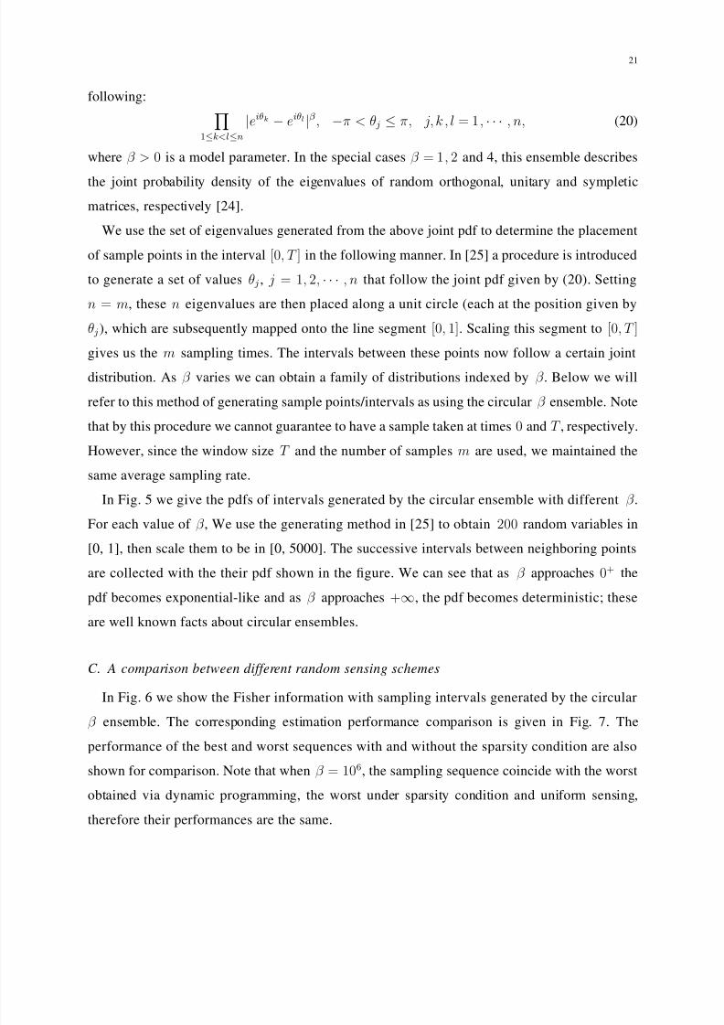
In Fig. 5 we give the pdfs of intervals generated by the circular ensemble with different β .

For each value of β , We use the generating method in [25] to obtain 200 random variables in

[0, 1], then scale them to be in [0, 5000]. The successive intervals between neighboring points

are collected with the their pdf shown in the figure. We can see that as β approaches 0+ the

pdf becomes exponential-like and as β approaches +∞, the pdf becomes deterministic; these

are well known facts about circular ensembles.

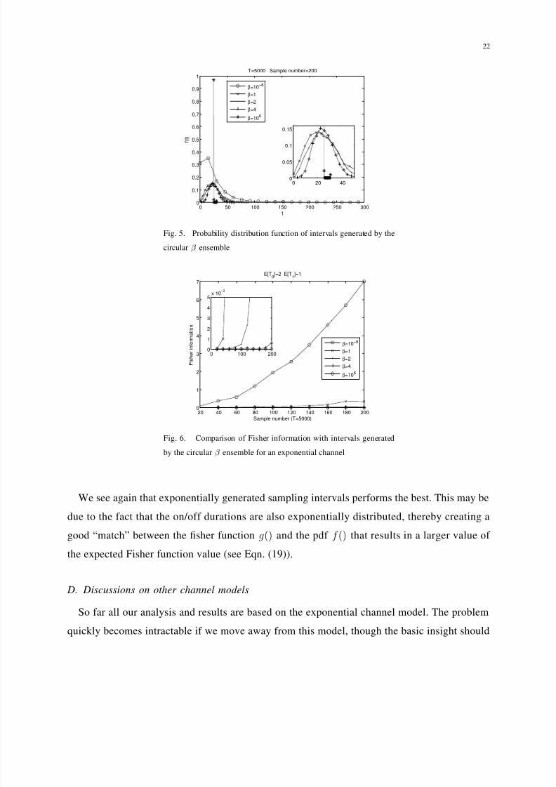
C. A comparison between different random sensing schemes

In Fig. 6 we show the Fisher information with sampling intervals generated by the circular

β ensemble. The corresponding estimation performance comparison is given in Fig. 7. The

performance of the best and worst sequences with and without the sparsity condition are also

shown for comparison. Note that when β = 106, the sampling sequence coincide with the worst

obtained via dynamic programming, the worst under sparsity condition and uniform sensing,

therefore their performances are the same.



22

0 50 100 150 200 250 3000

0.1

0.2

0.3

0.4

0.5

0.6

0.7

0.8

0.9

1

t

f ( t )

T=5000 Sample number=200

0 20 400

0.05

0.1

0.15

β=10−6

β=1

β=2

β=4

β=106

Fig. 5. Probability distribution function of intervals generated by the

circular β ensemble

20 40 60 80 100 120 140 160 180 200

0

1

2

3

4

5

6

7


F i s h e r i n f o r m a t i o n

E[T0]=2 E[T1]=1

0 100 2000

1

2

3

4

5x 10

−3

β=10

−6

β=1

β=2

β=4

β=106

Fig. 6. Comparison of Fisher information with intervals generated

by the circular β ensemble for an exponential channel

We see again that exponentially generated sampling intervals performs the best. This may be

due to the fact that the on/off durations are also exponentially distributed, thereby creating a

good “match” between the fisher function g() and the pdf f () that results in a larger value of

the expected Fisher function value (see Eqn. (19)).

D. Discussions on other channel models

So far all our analysis and results are based on the exponential channel model. The problem

quickly becomes intractable if we move away from this model, though the basic insight should



23

20 40 60 80 100 120 140 160 1800

5

10

15

20

25

30

35


1 / θ 0

E[T0]=2 E[T

1]=1

Actual value

β=10−6

(exponential)

β=1

β=2

β=4

β=106

(uniform)


Best by DP

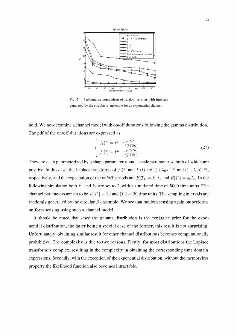
Fig. 7. Performance comparison of random sensing with intervals

generated by the circular β ensemble for an exponential channel

hold. We now examine a channel model with on/off durations following the gamma distribution.

The pdf of the on/off durations are expressed as

f 1(t) = tk1−1 e−t/λ1

λk11 Γ(k1)

f 0(t) = tk0−1 e−t/λ0

λk00 Γ(k0)

.(21)

They are each parameterized by a shape parameter k and a scale parameter λ, both of which are

positive. In this case, the Laplace transforms of f 0(t) and f 1(t) are (1+λ0s)−k0 and (1+λ1s)−k1,

respectively, and the expectation of the on/off periods are E [T 1] = k1λ1 and E [T 0] = k0λ0. In the

following simulation both k1 and k0 are set to 2, with a simulated time of 5000 time units. The

channel parameters are set to be E [T 1] = 10 and [T 0] = 20 time units. The sampling intervals are

randomly generated by the circular β ensemble. We see that random sensing again outperforms

uniform sensing using such a channel model.

It should be noted that since the gamma distribution is the conjugate prior for the expo-

nential distribution, the latter being a special case of the former, this result is not surprising.

Unfortunately, obtaining similar result for other channel distributions becomes computationallyprohibitive. The complexity is due to two reasons. Firstly, for most distributions the Laplace

transform is complex, resulting in the complexity in obtaining the corresponding time domain

expressions. Secondly, with the exception of the exponential distribution, without the memoryless

property the likelihood function also becomes intractable.



24

0 50 100 150 200 250 30015

20

25

30

35

40

45

50

55

60

65


2 λ 0

Gamma distribution: E[T0]=20 E[T

1]=10 k

1=k

0=2

Actual value

β=10−6 (exponential)

β=1

β=2

β=4

β=106

(uniform)

Fig. 8. Performance comparison of random sampling with intervals

generated by the circular β ensemble for gamma channel model

V I. ADAPTIVE RANDOM SENSING FOR PARAMETER TRACKING

Using insights we have obtained on uniform sensing and random sensing, we now present a

method of estimating and tracking a time-varying parameter. This is a moving window based

estimation scheme, where the overall sensing duration T is divided into windows of lengths

T w. In each window samples are taken and an estimate produced at the end of that window.

This estimate is then used to determine the optimal number of samples to be taken in the next

window. This method will be referred to as the adaptive random sensing scheme. The adaptivenature of the scheme comes from adjusting the number of samples taken in each window based

on past estimates.

Specifically, at the end of the i-th window of T w, we obtain the ML estimate θ(i)0 and u(i)

based on samples collected during that window. Now assuming that we will use uniform sensing

in the (i + 1)th window with a sampling interval ∆t p, and assuming that θ(i)0 and u(i) are the true

parameter values in the (i + 1)th window, we can obtain the expectation of the next estimate,

denoted as θ(i+1)0 , as a function of (T w, ∆t p, u(i), θ

(i)0 ). The optimal sampling interval ∆t(i+1) p for

the (i + 1)th window is then calculated as follows:

∆t(i+1) p = arg min∆tp

|θ(i+1)0 − θ(i)0 | − ε

, (22)

where ε is an error factor introduced to lower bound the minimizing interval ∆t(i+1) p . Without

this factor the interval will end up being very small, i.e., requiring a large number of samples for



25

the next window. The intuition behind the above formula is that assuming the channel parameters

are relatively slow varying in time, the estimate from the previous window θ(i)0 may be viewed

as true. So for the next window we would like to find the sampling interval that allows us to

get as close as possible to this value subject to an error.

Note that the above calculation relies on the availability of θ(i+1)0 , a quantity obtained assuming

uniform sampling will be used in the next window. In the actual execution of the algorithm, we

simply use this to obtain ∆t(i+1) p as shown above. This gives us the desired number of samples

to be taken in the next window: M (i+1) = ⌈T w/∆t(i+1) p ⌉. Following this, random sensing is used

to generate M (i+1) random sampling times within the next window. An estimate is then made

and this process repeats.

It remains to show how θ(i+1)0 is obtained. As mentioned earlier, when the on/off periods are

exponentially distributed there is a simple closed-form solution to the ML estimator. This was

calculated in [5] and we will use that result directly below. Specifically, with M = ⌈T w/∆t p⌉samples uniformly taken, the estimate of channel utilization u is given by u = 1

M

M i=1 zi. The

estimate of θ0 is given by

θ0 = − u

∆t pln[

−B +√

B2 − 4AC

2A], (23)

where

A = (u

−u2)(M

−1)

B = −2A + (M − 1) − (1 − u)n0 − un3

C = A − un0 − (1 − u)n3

. (24)

Here n0/n1/n2/n3 denotes the number of (0 → 0)/(0 → 1)/(1 → 0)/(1 → 1) transitions out

of the total (M − 1) transitions. Their respective expectations are given by

E [n0] = M (1 − u)P 00(∆t p; θ0), E [n2] = MuP 10(∆t p; θ0),

E [n1] = M (1 − u)P 01(∆t p; θ0), E [n3] = MuP 11(∆t p; θ0).(25)

Taking these quantities into (24) and (23), we obtain the expectation of θ0, θ0, which is a function

of (T w, ∆t p, u , θ0). Replacing u with u(i), θ0 with θ(i)0 , and θ0 with θ

(i+1)0 we obtain the desired

result.

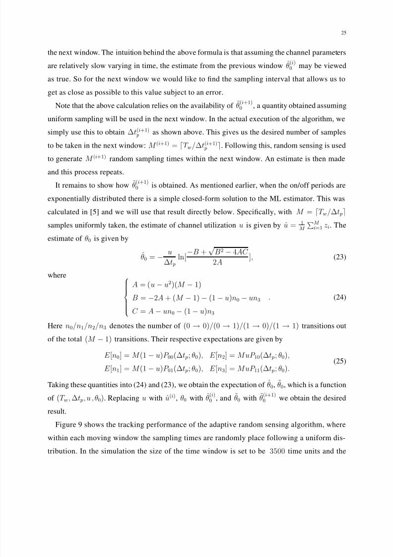
Figure 9 shows the tracking performance of the adaptive random sensing algorithm, where

within each moving window the sampling times are randomly place following a uniform dis-

tribution. In the simulation the size of the time window is set to be 3500 time units and the



26

error factor ε is set at 1. In Figure 9(a) the channel parameter E [T 0] varies as a step function:

starting from 6 time units, it is increased by 5 every 30000 time units, while E [T 1] is set to

E [T 0]/2. In Figure 9(b) the channel parameter changes more smoothly as shown. The dashed line

represents the actual channel parameter. For comparison purpose we also include the results from

an adaptive uniform sensing algorithm. These are obtained by following the exact same adaptive

procedure outlined above, with the only difference that in the i-th window uniform sensing is

used, instead of random sensing, with a constant sampling interval of ∆t(i) p . We see that the

estimation under adaptive random sensing (RS) can closely track the time-varying channel, and

clearly outperforms adaptive uniform sensing (US) at short on/off periods.

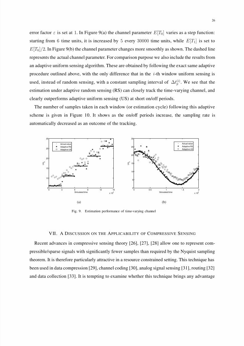
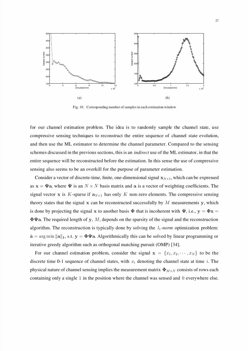
The number of samples taken in each window (or estimation cycle) following this adaptive

scheme is given in Figure 10. It shows as the on/off periods increase, the sampling rate is

automatically decreased as an outcome of the tracking.

0 3 6 9 12 15

x 104

5

10

15

20

25

30

Simulated time

1 / θ 0

Actual value

Adaptive RS

Adaptive US

(a)

0 0.5 1 1.5 2

x 105

0

5

10

15

20

25

30

Simulated time

1 / θ 0

Actual value

Adaptive RS

Adaptive US

(b)

Fig. 9. Estimation performance of time-varying channel

VII. A DISCUSSION ON THE APPLICABILITY OF COMPRESSIVE SENSING

Recent advances in compressive sensing theory [26], [27], [28] allow one to represent com-

pressible/sparse signals with significantly fewer samples than required by the Nyquist sampling

theorem. It is therefore particularly attractive in a resource constrained setting. This technique has

been used in data compression [29], channel coding [30], analog signal sensing [31], routing [32]

and data collection [33]. It is tempting to examine whether this technique brings any advantage



27

0 3 6 9 12 15

x 104

150

200

250

300

350

400

450

500

Simulated time

S a m p

l e n u m b e r

(a)

0 0.5 1 1.5 2

x 105

100

150

200

250

300

350

Simulated time

S a m p

l e n u m b e r

(b)

Fig. 10. Corresponding number of samples in each estimation window

for our channel estimation problem. The idea is to randomly sample the channel state, use

compressive sensing techniques to reconstruct the entire sequence of channel state evolution,

and then use the ML estimator to determine the channel parameter. Compared to the sensing

schemes discussed in the previous sections, this is an indirect use of the ML estimator, in that the

entire sequence will be reconstructed before the estimation. In this sense the use of compressive

sensing also seems to be an overkill for the purpose of parameter estimation.

Consider a vector of discrete-time, finite, one-dimensional signal xN ×1, which can be expressed

as x = Ψa, where Ψ is an N × N basis matrix and a is a vector of weighting coefficients. The

signal vector x is K -sparse if aN ×1 has only K non-zero elements. The compressive sensing

theory states that the signal x can be reconstructed successfully by M measurements y, which

is done by projecting the signal x to another basis Φ that is incoherent with Ψ, i.e., y = Φx =

ΦΨa. The required length of y, M , depends on the sparsity of the signal and the reconstruction

algorithm. The reconstruction is typically done by solving the l1-norm optimization problem:

a = arg min a1, s.t. y = ΦΨa. Algorithmically this can be solved by linear programming or

iterative greedy algorithm such as orthogonal matching pursuit (OMP) [34].For our channel estimation problem, consider the signal x = {x1, x2, · · · , xN } to be the

discrete time 0-1 sequence of channel states, with xi denoting the channel state at time i. The

physical nature of channel sensing implies the measurement matrix ΦM ×N consists of rows each

containing only a single 1 in the position where the channel was sensed and 0 everywhere else.



28

Specifically, a 1 in the position (i, j) means that the ith measurement was taken at time j. In

addition, there can only be one measurement taken at time j, i.e., no two rows can have a 1

in the same column. As M < N in general (or it wouldn’t be compressive sensing), there will

be exactly N −

M empty (all-0) columns, making the matrix extremely sparse. This poses a

significant challenge since in general the Φ matrix is required to be dense (though randomly

generated), with at least one non-zero entry in each column.

For the reconstruction to be successful, two conditions need to be satisfied: the signal needs

be sparse in some domain (i.e., the existence of a Ψ such that a is sufficiently sparse), and

the two matrices Φ and Ψ need to be incoherent. Due to the binary property of the channel

state sequence, it’s difficult to find a basis matrix Ψ that has dense entities. As a result we have

two very sparse matrices and they are highly coherent. For these reasons we have not found

compressive sensing to have an advantage in our channel estimation problem.

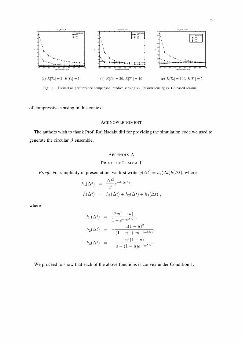
Figure 11 shows some comparison results. In the simulation of compressive sensing based

estimation, we reconstruct the original state sequence using Harr wavelet basis. All other con-

ditions remain the same as in previous sections. The time window is set to 4096 time units.

Overall compressive sensing based estimation dose not compare favorably with uniform sensing

and random sensing, due to the coherence problem between the two matrices. It remains an

interesting problem to find a good basis matrix that can both sparsify x and at the same time be

sufficiently incoherent with the measurement matrix. A similar difficulty was noted in [32] in

trying to use compressive sensing for a data gathering problem. A number of commonly used

transformations were considered, and it was found that, with real data sets, none of them was

able to sparsify the data while being at the same time incoherent with the routing matrix.

VIII. CONCLUSION

In this paper we studied sensing schemes for a channel estimation problem under a sparsity

condition. Using Fisher information as a performance measure, we derived the best and worst

sensing sequences both with and without the sparsity condition. These sequences, while not ex-

actly implementable, provide significant insights as well as useful benchmarks. We then examined

the performance of random sensing schemes, by comparing a family of distributions generated

by the circular β ensemble. Using these insights, an adaptive random sensing scheme was

proposed to effectively track time-varying channel parameters. We also discuss the applicability



29

100 200 300 400 500 600 700 800 900 10000

10

20

30

40

50

60

70

80

90

100

Average sample number

1 / θ

0

E[T0]=2 E[T

1]=1

Actual value

RS

US

CS

(a) E [T 0] = 2, E [T 1] = 1

100 200 300 400 500 600 700 800 900 100010

20

30

40

50

60

70

80

90

100

110


1 / θ

0

E[T0]=20 E[T

1]=10

Actual value

RS

US

CS

(b) E [T 0] = 20, E [T 1] = 10

100 200 300 400 500 600 700 800 900 10000

100

200

300

400

500

600

700

800

900


1 / θ

0

E[T0]=100 E[T

1]=5

Actual value

RS

US

CS

(c) E [T 0] = 100, E [T 1] = 5

Fig. 11. Estimation performance comparison: random sensing vs. uniform sensing vs. CS based sensing

of compressive sensing in this context.

ACKNOWLEDGMENT

The authors wish to thank Prof. Raj Nadakuditi for providing the simulation code we used to

generate the circular β ensemble.

APPENDIX A

PROOF OF LEMMA 1

Proof: For simplicity in presentation, we first write g(∆t) = ho(∆t)h(∆t), where

ho(∆t) = ∆t2u2

e−θ0∆t/u,

h(∆t) = h1(∆t) + h2(∆t) + h3(∆t) ,

where

h1(∆t) =2u(1 − u)

1 − e−θ0∆t/u,

h2(∆t) = − u(1 − u)2

(1 − u) + ue−θ0∆t/u,

h3(∆t) = − u2

(1 − u)u + (1 − u)e−θ0∆t/u

.

We proceed to show that each of the above functions is convex under Condition 1.



30

We first show that ho(∆t) is strictly convex for ∆t > (2 +√

2)u/θ0. Under this condition and

noting 0 < u < 1 and θ0 > 0 we have

h′

o(∆t) =∆t

u2e−θ0∆t/u(2 − θ0∆t

u) < 0,

h′′

o(∆t) = e−θ0∆t/u

u2[(θ0∆t

u− 2)2 − 2] > 0.

Therefore for θ0∆tu > 2 +

√2, ho(∆t) is strictly convex. That h1(∆t) is strictly convex is

straightforward. Since 0 < u < 1 and θ0 > 0, we have:

h′

1(∆t) =−2(1 − u)θ0e−θ0∆t/u

(1 − e−θ0∆t/u)2< 0,

h′′

1(∆t) =2(1 − u)θ20e−θ0∆t/u(1 + e−θ0∆t/u)

u(1 − e−θ0∆t/u

)3

> 0.

Next we show that h2(∆t) is strictly convex for ∆t > uθ0

ln( u1−u). This condition is equivalent

to ue−θ0∆t/u < 1 − u. Under this condition and again noting 0 < u < 1 and θ0 > 0, we have

h′

2(∆t) =−u(1 − u)2θ0e−θ0∆t/u

[(1 − u) + ue−θ0∆t/u]2< 0,

h′′

2(∆t) =(1 − u)2θ20e−θ0∆t/u[(1 − u) − ue−θ0∆t/u]

[(1 − u) + ue−θ0∆t/u]3> 0.

Similarly, h3(∆t) is strictly convex under the condition ∆t > uθ0

ln(1−uu

), since

h′

3(∆t) =−u(1 − u)2θe−θ0∆t/u

[u + (1 − u)e−θ0∆t/u]2< 0,

h′′

3(∆t) =(1 − u)2θ2e−θ0∆t/u[u − (1 − u)e−θ0∆t/u]

[u + (1 − u)e−θ0∆t/u]3> 0.

Therefore under the condition ∆t > αu/θ0, h1, h2 and h3 are all monotonically decreasing

convex functions. It follows that h = h1 + h2 + h3 is also monotonically decreasing and convex.

Furthermore, for any ∆t > 0, ho(∆t) > 0, and h(∆t) > h(+∞) = 0. We can now show that g

is strictly convex under this condition:

g′′

(∆t) = (ho(∆t)h(∆t))′′

= h′′

o(∆t)h(∆t) + 2h′

o(∆t)h′

(∆t) + ho(∆t)h′′

(∆t) > 0 ,(26)



31

where the inequality holds because every term on the right hand side is positive under the

condition ∆t > αu/θ0 as summarized above.

REFERENCES

[1] S. Haykin, “Cognitive radio: brain-empowered wireless communications,” IEEE journal on selected areas in communica-

tions, vol. 23, pp: 201-220, Feb. 2005.

[2] K. Challapali, C. Cordeiro, and D. Birru, “Evolution of Spectrum-Agile Cognitive Radios: First Wireless Internet Standard

and Beyond,” Proceedings of ACM International Wireless Internet Conference, August 2006.

[3] I. F. Akyildiz, W.-Y. Lee, M. C. Vuran, and S. Mohanty, “NeXt generation dynamic spectrum access cognitive radio wireless

networks: A survey,” Computer Networks Journal (Elsevier), pp: 201-220, Sept. 2006.

[4] D. Cabric, S. M. Mishra, R. W. Brodersen, “Implementation issues in spectrum sensing for cognitive radios,” Proceedings

of Asilomar Conference on Signals, Systems and Computers, 2004.

[5] H. Kim and K. G. Shin, “Efficient discovery of spectrum opportunities with MAC-layer sensing in cognitive radio networks,”

IEEE Transactions on Mobile Computing, vol.7, no.5, pp: 533-545, May 2008.

[6] Q. Zhao, L. Tong, A. Swami, and Y. Chen, “Decentralized cognitive MAC for opportunistic spectrum access in ad hoc

networks: a POMDP framework,” IEEE Journal on Selected Areas in Communications , vol. 25, no. 3, pp: 589-599, Apr.

2007.

[7] M. Dong, L. Tong, and B. M. Sadler, “Information Retrieval and Processing in Sensor Networks: Deterministic Scheduling

Versus Random Access,“ IEEE Transactions on Signal Processiong, vol. 55, no. 12, pp: 5806-5820, 2007.

[8] H. Kim and K. G. Shin, “Fast Discovery of Spectrum Opportunities in Cognitive Radio Networks,” Proceedings of the 3rd

IEEE Symposia on New Frontiers in Dynamic Spectrum Access Networks (IEEE DySPAN), Oct. 2008.

[9] X. Long, X. Gan, Y. Xu, J. Liu, M. Tao, “An Estimation Algorithm of Channel State Transition Probabilities for Cognitive

Radio Systems,” Proceedings of Cognitive Radio Oriented Wireless Networks and Communications (CrownCom), 15-17

May 2008

[10] C. H. Park, S. W. Kim, S. M. Lim, M. S. Song, “HMM Based Channel Status Predictor for Cognitive Radio,” Proceedings

of Asia-Pacific Microwave Conference,11-14 Dec. 2007.

[11] A. A. Fuqaha, B. Khan, A. Rayes, M. Guizani, O. Awwad, G. Ben Brahim, “Opportunistic Channel Selection Strategy for

Better QoS in Cooperative Networks with Cognitive Radio Capabilities,” IEEE Journal on Selected Areas in Communications,

Vol. 26, No. 1, pp: 156-167, Jan. 2008.

[12] D. Chen, S. Yin, Q. Zhang, M. Liu and S. Li, “Mining Spectrum Usage Data: a Large-scale Spectrum Measurement Study,”

ACM MobiCom, September 2009, Beijing, China.

[13] P. J. Kolodzy, ”Cognitive radio fundamentals,” Proceedings of SDR Forum, Singapore, Apr. 2005.

[14] R. A. Fisher, “On the Mathematical Foundations of Theoretical Statistics,” Mathematical Foundations of Theoretical

Statistics vol. 222, pp: 309-368, 1922.

[15] D. R. Cox, Renewal Theory, Butler and Tanner,1967.

[16] J. Lee, J. Choi, H. Lou, “Joint Maximum Likelihood Estimation of Channel and Preamble Sequence for WiMAX Systems,”

IEEE Transactions on Wireless Communications, Vol. 7, No. 11, pp: 4294-4303, Nov. 2008.

[17] J. Wang, A. Dogandzic, A. Nehorai, “Maximum Likelihood Estimation of Compound-Gaussian Clutter and Target

Parameters,” IEEE Transactions on Signal Processing, vol. 54, no.10, pp: 3884-3898 Oct. 2006.



32

[18] U. Orguner, M. Demirekler, “Maximum Likelihood Estimation of Transition Probabilities of Jump Markov Linear Systems,”

IEEE Transactions on Signal Processing, vol. 56, no. 10, Part 2, pp: 5093-5108 Oct. 2008.

[19] H.A. Cirpan, M.K. Tsatsanis, “Maximum likelihood blind channel estimation in the presence of Doppler shifts,” IEEE

Transactions on Signal Processing, vol. 47, no. 6, pp: 1559-1569, Jun. 1999.

[20] M. Abuthinien, S. Chen, L. Hanzo, “Semi-blind Joint Maximum Likelihood Channel Estimation and Data Detection for

MIMO Systems,” IEEE Signal Processing Letters, vol. 15, pp: 202-205, 2008.

[21] A.W. van der Vaart, Asymptotic Statistics (Cambridge Series in Statistical and Probabilistic Mathematics) (1998)

[22] R. A. Fisher, The Design of Experiments, Oliver and Boyd, Edinburgh, 1935.

[23] J.A. Legg, D.A. Gray, “Performance Bounds for Polynomial Phase Parameter,” IEEE Transactions on Signal Processing,

vol. 48, no.2, pp: 331-337 Feb. 2000.

[24] M. L. Mehta, Random matrices. Elsevier/Academic Press, 2004.

[25] A. Edelman, B.D. Sutton, “The Beta-Jacobi Matrix Model, the CS Decomposition, and Generalized Singular Value

Problems,” Foundations of Computational Mathematics, vol. 8 , no. 2, pp: 259-285, May 2008.

[26] D. Donoho, “Compressed sensing,” IEEE Transactions on Information Theory, vol. 52, no. 4, pp: 4036-4048, 2006.

[27] E. Candes and T. Tao, “Near optimal signal recovery from random projections: Universal encoding strategies?” IEEE Transactions on Information Theory, vol. 52, no. 12, pp: 5406-5425, 2006.

[28] E. Candes, J. Romberg, and T. Tao, “Robust uncertainty principles: Exact signal reconstruction from highly incomplete

frequency information,” IEEE Transactions on Information Theory, vol. 52, no. 2, pp: 489-509, 2006.

[29] D. Baron, M.B. Wakin, M.F. Duarte, S. Sarvotham, and R.G. Baraniuk, “Distributed compressed sensing,” 2005, Preprint.

[30] E. Candes and T. Tao, “Decoding by linear programming,” IEEE Transactions Information Theory, vol. 51, no. 12, pp:

4203-4215, Dec. 2005.

[31] Z. Tian and G. Giannakis, “Compressed Sensing for Wideband Cognitive Radios,” Proceedings of IEEE Internation

Conference on Acoustics, Speech and Signal Processing (ICASSP) , Vol. 4, pp: 1357-1360, Honolulu, Apr. 2007.

[32] G. Quer, R. Masiero, D. Munaretto, M. Rossi, J. Widmer and M. Zorzi, “On the Interplay Between Routing and Signal

Representation for Compressive Sensing in Wireless Sensor Networks,” Information Theory and Applications Workshop

(ITA 2009), San Diego, CA.

[33] C. Luo, F. Wu, C. W. Chen and J. Sun, “Compressive Data Gathering for Large-Scale Wireless Sensor Networks,” ACM

MobiCom, September 2009, Beijing, China.

[34] J. A. Tropp, A. C. Gilbert, “Signal Recovery From Random Measurements Via Orthogonal Matching Pursuit,” IEEE

Transactions on Information Theory, vol. 53, no. 12, pp: 4655-4666, 2007.

Documents

Channel Sense