Embed Size (px)
Citation preview
CHANGING SOIL DEGRADATION TRENDS IN SENEGAL
WITH CARBON SEQUESTRATION PAYMENTS
by
Kara Michelle Gray
A thesis submitted in partial fulfillment of the
requirements for the degree
of
Master of Science
in
Applied Economics
MONTANA STATE UNIVERSITY Bozeman, Montana
January, 2005

©COPYRIGHT
by
Kara Michelle Gray
2005
All Rights Reserved

ii
APPROVAL
of a thesis submitted by
Kara Michelle Gray
This thesis has been read by each member of the thesis committee and has been found to be satisfactory regarding content, English usage, format, citations, bibliographic style, and consistency, and is ready for submission to the College of Graduate Studies.
Dr. John Antle (Committee Chair)
Approved for the Department of Agricultural Economics and Economics
Dr. Richard Stroup Approved for the College of Graduate Studies
Dr. Bruce McLeod
iii
STATEMENT OF PERMISSION TO USE
In presenting this thesis in partial fulfillment of the requirements for a master’s
degree at Montana State University, I agree that the Library shall make it available to
borrowers under rules of the Library.
If I have indicated my intention to copyright this thesis by including a copyright
notice page, copying is allowable only for scholarly purposes, consistent with “fair use” as
prescribed in the U.S. Copyright Law. Requests for permission for extended quotation from
or reproduction of this thesis in whole or in parts may be granted only by the copyright
holder.
Kara M. Gray
January 10th, 2005

iv
ACKNOWLEDGMENTS
I would like to thank the many people who supported, pushed and pulled me
throughout my time at Montana State University. I’m grateful to my professors, who
taught with considerate rigor, fielded ceaseless questions, and who generally had the
grace to not mock our ignorance. I’d like to thank the support staff in the department –
for fixing my computer, for deciphering procedures and finding information for me, and
for their wonderful welcoming company. I’d like to thank my classmates, who provided
me with hours of comic relief - at the Kaiser table, on the ski hill, on road trips, and
during heated bullpen debates. I couldn’t have moved so many times without them.
Writing this thesis was one of the most challenging things I’ve ever done. I would
like to thank my committee members, Dr. Dave Buschena and Dr. John Marsh, for their
time and effort, and my committee chair, Dr. John Antle, for his insight, patience and
support. My friends, family and cohort, provided valuable cheerleading and cajoling as
necessary. Thanks.

v
TABLE OF CONTENTS
1. NEW PERSPECTIVES ON CREATING INCENTIVES FOR THE ADOPTION OF SUSTAINABLE SOIL MANAGEMENT PRACTICES…..…..1
INTRODUCTION ................................................................................................................... 1 FOOD SECURITY, AGRICULTURAL PRODUCTION AND SOIL DEGRADATION IN AFRICA ..... 3
Population Pressure, Natural Resources and the Rational Farmer..............................5 Soil Degradation and Soil Carbon Sequestration........................................................9
THESIS OBJECTIVES .......................................................................................................... 16
2. THE FARMER AND THE CARBON CONTRACT………………………………18
NUTRIENT MINING, AND THE ROLE OF FERTILIZER AND CROP RESIDUES IN AGRICULTURAL SYSTEMS................................................................................................. 18
Input Usage & the Rational Farmer ..........................................................................21 DYNAMICS, ADOPTION THRESHOLDS AND THE ROLE OF INCENTIVES............................. 25 CARBON CONTRACTS FOR FERTILIZER AND RESIDUE INCORPORATION .......................... 28
3. THE SIMULATION APPROACH…………………………………...……………...33
MODELING COMPLEX SYSTEMS........................................................................................ 33 Integrated Assessment for Agricultural Production Systems....................................34 Methods.....................................................................................................................36 Crop and Carbon Models. .........................................................................................37 Economic Models: The Econometric Process Simulation Model.............................40
SENSITIVITY ANALYSIS OF SOIL CARBON MANAGEMENT USING INTEGRATED ASSESSMENT MODELS. ..................................................................................................... 42
Scenario Analysis......................................................................................................43
4. CASE STUDY: SENEGAL…………………………………………………………...45
GEOGRAPHY...................................................................................................................... 45 HISTORICAL BACKGROUND .............................................................................................. 49 CRISIS IN SENEGAL ........................................................................................................... 53 INPUT MARKETS AND POLICIES ........................................................................................ 58
Crop Residue.............................................................................................................60 Land Tenure ..............................................................................................................63 Private Markets .........................................................................................................64
DISCUSSION....................................................................................................................... 65

vi
TABLE OF CONTENTS - CONTINUED
5. MODEL IMPLEMENTATION, SCENARIOS & RESULTS…………...………..66
THE NIORO DATASET........................................................................................................ 67 STRUCTURE OF THE ANALYSIS ......................................................................................... 72
Biophysical Parameters: Inherent Productivity.........................................................77 Econometric Specification and Estimation of Groundnut and Millet Production Models.......................................................................................................................78 Supply Equations ......................................................................................................88
CARBON CONTRACT & POLICY ANALYSIS ....................................................................... 91 Implementation Issues...............................................................................................92 Contract Design & Incentives. ..................................................................................92
RESULTS OF SIMULATION ................................................................................................. 95 Base Policy Results. ..................................................................................................95
SENSITIVITY ANALYSIS..................................................................................................... 98 Sensitivity Analysis Results....................................................................................101 Discussion ...............................................................................................................109
6. CONCLUSION…………………………………………………………….…………112
BIBLIOGRAPHY...................................................................................................... 115

vii
LIST OF TABLES
Table Page
1. Additional Benefits of Enhancing the Soil Carbon Pool ..................................................12
2. Regions of the Groundnut Basin of Senegal.....................................................................48
3. Population Statistics..........................................................................................................57
4. Average Yields and Revenues from the 2000 ENEA Dataset ..........................................62
5. Sampled Variables Used in Analysis (Nioro Region of Senegal, 2000)...........................69
6. Sampled Variables Used in Analysis................................................................................70
7. OLS Results of Millet Seed Price Distribution.................................................................73
8. OLS Estimates of Groundnut Seed Price Parameters .......................................................73
9. OLS Estimates of Fungicide Price Parameters .................................................................74
10. OLS Estimation of Mineral Fertilizer Price Parameters ...................................................74
11. OLS Estimates of Farm Size Parameters ..........................................................................75
12. OLS Estimates of Field Area Parameters .........................................................................75
13. OLS Estimates of Groundnut Seed Demand Parameters..................................................80
14. OLS Estimates of Labor Demand Parameters in Groundnut Fields .................................80
15. OLS Estimates of Millet Seed Demand Parameters .........................................................80
16. OLS Estimates of Labor Demand Parameters in Millet Fields.........................................81
17. Probit Model For Fertilizer Use in Groundnut Fields (Modeling the Probability of No Fertilizer Usage: X6d1=0) ...................................................................82
18. Probit Model For Fertilizer Use in Millet Fields (Modeling the Probability of No Fertilizer Usage: X6d2=0) ......................................................................................83
19. OLS Estimates of Groundnut Fertilizer Demand Parameters (Where X6>0)...................86
20. OLS Estimates of Millet Fertilizer Demand Parameters (Where X6>0) ..........................86
21. Estimated Groundnut Fungicide Use Discrete Choice and Input Demand Parameters.........................................................................................................................87
22. OLS Estimated Groundnut Grain Supply Parameters.......................................................89
23. OLS Estimated Groundnut Residue Supply Parameters...................................................89
24. OLS Estimated Millet Grain Supply Parameters ..............................................................90
25. Carbon Policy Management Practice Requirements.........................................................91
26. Scenario Guide..................................................................................................................99

viii
LIST OF FIGURES
Figure Page
1. Average Carbon Stocks Over Time, Given 9 Different Management Practices............... 13
2. The Cycle of Soil Depletion, Food Insecurity and Agronomic and Environmental Quality...................................................................................................... 14
3. Carbon Payments, and the Steps Towards Food Security and Sustainability................... 15
4. Distribution and Probability of Fertilizer Usage in the Senegal ENEA Sample............... 20
5. Fertilizer Usage with Market Distortions ......................................................................... 23
6. Average Annual Changes in SOC with Carbon Contracts On A Sample Field (Generated By the Dssat/Century Model; T=20 Years) .......................................... 24
7. Net Revenue and Opportunity Costs Associated with Fertilizer Usage ........................... 30
8. Econometric-Process Model ............................................................................................. 35
9. Integrated Assessment Model of Carbon Sequestration ................................................... 36
10. Inherent Productivity Levels Given 9 Different Management Practices .......................... 38
11. Time Paths of Carbon Changes in A Field ....................................................................... 39
12. Structure of the Econometric-Process Model ................................................................... 41
13. Map of Africa.................................................................................................................... 46
14. Crop Area in Senegal, 2001/2002 Crop Year ................................................................... 46
15. Map of Senegal, and Senegal’s Groundnut Basin............................................................. 47
16. Farmgate and World Groundnut Prices ............................................................................ 51
17. Production of Groundnuts and Millet per Capita (Diourbel Region), tonnes ................... 54
18. Historic Rainfall Levels in Senegal's Groundnut Basin.................................................... 55
19. Millet Yields in the Diourbel Region................................................................................ 56
20. Fertilizer Subsidy Rate in Senegal (% of Full Cost)......................................................... 59
21. Kilograms of Groundnuts Necessary to Purchase 1 kg of Mineral Fertilizer ................... 60
ixLIST OF FIGURES - CONTINUED
Figure Page
22. Meat Prices in Senegal...................................................................................................... 61
23. Changes in Livestock Owned, 1960-96, Diourbel Region ............................................... 62
24. Structure of the Econometric-Process Simulation Model................................................. 71
25. Inherent Productivity Data, By Soil Type and Crop......................................................... 78
26. Crop Yield and Carbon Sequestration Returns to Fertilizer Use ...................................... 88
27. Carbon Supply with 6 Residue-Incorporating Carbon Contract Policies ......................... 96
28. Detail of Carbon Supply with 6 Residue-Incorporating Carbon Contract Policies ............................................................................................................... 97
29. Contract Participation in 6 Residue Incorporating Carbon Contract Policies................... 97
30. Carbon Supply with Different Labor Costs of Residue Incorporation. .......................... 101
31. Carbon Supply Sensitivity to Pparm Levels ................................................................... 102
32. Carbon Supply Sensitivity to Contract Transaction Costs.............................................. 103
33. Contract Participation Sensitivity to Contract Transaction Cost Levels......................... 104
34. Participation Sensitivity to Entry and Exit Restrictions.................................................. 105
35. Crop Choice Composition with and Without Entry/Exit Restrictions ............................ 105
36. Contract "I" Participation with 3 Different Fertilizer Response Functions (X6kink).......................................................................................................................... 106
37. Carbon Supply with 3 Different Fertilizer Response Functions (X6kink) ..................... 107
38. Contract Participation Sensitivity to Groundnut Residue Price (Pb1c) .......................... 108
39. Carbon Supply Sensitivity to Groundnut Residue Price (Pb1c) ..................................... 108
40. Carbon Stocks with "A" and "I" Management Requirements......................................... 110
41. Average Carbon Stocks, Given Different Carbon Prices and Corresponding Adoption Rates of Type "I" Contract Requirements....................................................... 110
42. Average Inherent Productivity, Given Three Carbon Prices and Corresponding Adoption Rates of Type "I" Contract Requirements.............................. 111

xABSTRACT
In Sudo-Sahelian Africa, erosion and nutrient mining are prominent causes of soil
degradation. In Senegal, harvesting grains and crop residue from the land impact heavily on soil carbon content, while the insufficient replacement of soil nutrients with fertilizers contributes to negative nutrient balances. Given the economic perspective of the rational farmer and the dynamic nature of crop and soil management issues, this thesis used a regional case study in the Groundnut Basin of Senegal to do the following: describe and assess economic incentives specific the to the case study region; model the farmer's production and decision making process; design carbon contract policies and model them within the farmer’s decision making process; simulate the interaction between the current agricultural marketplace and potential carbon policies; and to assess the role that carbon sequestration could play in helping the region deal with soil degradation problems, if and when international action is taken to reduce greenhouse gas emissions. Information from farmers in the region indicates that several factors constrain fertilizer use, including financial constraints and market imperfections. The result of these constraints is to reduce the productivity and increase the farm gate cost of fertilizers. The results of the simulation supported this hypothesis. Using data from the Groundnut Basin in Senegal, and employing an econometric-process simulation model, this study found that some carbon contracts could be used to reduce losses in soil carbon and productivity; however, only at high carbon prices ($180 USD/t carbon and higher). Transactions costs, the additional labor costs associated with residue incorporation, and groundnut residues prices all strongly influenced the results of the carbon contract policies, particularly where carbon prices are less than $100/t.

1
CHAPTER 1
NEW PERSPECTIVES ON CREATING INCENTIVES FOR THE ADOPTION OF
SUSTAINABLE SOIL MANAGEMENT PRACTICES
Introduction
Declining soil organic carbon content, and resultant declines in soil fertility, are
problems for many of the world’s agricultural production systems (Oldeman, 1990)
Although volumes of soil conservation research focus on this problem and alternative
sustainable practices, this trend continues in many parts of the world today, notably in Sub-
Saharan Africa (SSA).
A key process in many unsustainable agricultural systems is degradation of soils
through loss of soil organic carbon (SOC). With cultivation, soils may lose 50% or more
of their organic carbon content, depending on soil conditions and agricultural practices.
Consequently, there is a potential to increase SOC in most cultivated soils. Soil carbon
sequestration is defined as using plant photosynthesis to capture carbon dioxide (CO2) from
the atmosphere, and put it into soil carbon stocks. This is can be achieved by a variety of
management practices including: increasing cropping intensity and fertilization; mulch
farming; conservation tillage; cover crops; integrated nutrient management; and
agroforestry (Lal, 2004).
2
The cycle of depletion of soil organic matter, declining crop yields, poverty and
food insecurity, and soil and environmental degradation could be broken by improving soil
fertility through enhancement of the SOC pool (Lal, 2004). Incentive mechanisms to
encourage carbon sequestration could alleviate those problems, while satisfying
international goals of greenhouse gas mitigation. A key question that needs to be answered
before implementation is: at what cost can SOC losses be slowed or reversed?
There are several crucial factors to be considered in order to evaluate carbon
sequestration’s potential as an instrument to break the cycle of soil degradation. These
include: the design of institutions that would convert global demand for reduced
greenhouse gases into incentives for carbon sequestration (Young, 2003); externalities or
“co-benefits” of new practices, such as erosion reduction, improved pollution control, and
nutritional improvements; and, the technical SOC storage potential of soils. In the final
case, although the SOC storage potential factor may be high, it could also be very
expensive to reach. As a result, we must analyze both the SOC storage potential and the
economic returns to adapting sequestering practices.
Contract design will play an important role in the successful implementation of a
carbon sequestering initiative, as the payments must convey the intended incentives to large
numbers of farmers managing small farms.
A number of studies have estimated the technical and economic potential for soil
carbon sequestration in the United States (e.g., Pautsch et al. 2001; Antle et al. 2001, 2003;
McCarl and Schneider 2001). Few studies have assessed soil carbon sequestration potential
in developing countries. Antle et al. (2003) analyzed the potential for terracing and

3
agroforestry to sequester carbon in hillside agriculture in Peru. Tschakert (2004) estimated
carbon sequestration rates and economic returns to different management techniques for the
Senegal groundnut basin, establishing the link between increased fertilizer usage, residue
incorporation and reduced soil degradation.
Using simulation analysis, this thesis will examine the economic feasibility of
slowing or reversing soil degradation through carbon sequestration payments in the
Groundnut Basin of Senegal, a region typical of dryland subtropical Sub Saharan Africa.
Farmers’ participation in carbon sequestering contracts will be simulated with
consideration of existing markets and institutions. Following the examination of the
feasibility of carbon sequestration, we will simulate carbon supply under a variety of policy
and technology scenarios, and assess the potential for farmers’ participation in carbon
contracts to slow or reverse the trend towards soil degradation in the region.
Food Security, Agricultural Production and Soil Degradation in Africa
Africa’s population growth rate is the highest on the planet, while its agricultural
productivity growth has fallen behind population growth and in some cases has declined
absolutely. Approximately 180 million Africans suffer from malnutrition – an increase of
100% since 1970. Malnutrition exacerbates health problems such as HIV/AIDS, malaria
and tuberculosis (Sanchez, 2002). The USDA Economic Research Service projects that the
number of hungry people in SSA will rise in proportion to its anticipated population growth
over the next decade (2004).
4
Addressing issues such as child survival, disease management, foreign investment,
trade barriers and debt-relief are all significant and necessary to unraveling Africa's
problems. However, interested parties cannot solve Africa’s woes without first (or also)
addressing agricultural productivity. As an economic sector, agriculture engages 70% of all
Africans. In Sub-Saharan Africa, agriculture is the primary source of food, livelihood and
foreign exchange earnings (Badian and Delago, 1995). In many rural areas, households
depend upon their own production for food and fodder. Imports are a minor part of total
food supplies; making domestic food production integral to food security in the region
(Wiebe et al., 2001). The food aid and foreign exchange earning capacity of West African
countries are projected to decrease, the latter due to decreased tourism, low savings and
investment rates, poor infrastructure and the growing burden of the HIV/AIDS epidemic
(ERS, 2004).
Other regions of the world have reaped significant agricultural production gains
through and since the Green Revolution, while African agriculture (particularly in the Sub
Sahelian region) has floundered. Even though technology has improved over time, many of
Africa's countries have been less able to actualize the benefits. Sanchez (2002) cites a
recent study, stating that while adoption rates of improved crop varieties during the last 38
years have been similar in Asia, Latin America, the Middle East, and Sub-Saharan Africa,
varieties are responsible for 66% to 88% of crop yield increases in the first three regions,
but for only 28% in Sub-Saharan Africa.
5
Soil fertility depletion is regarded as the primary biophysical factor that limits food
production on most African small farms (Drechsel et al., 2001).What is causing this trend,
and how can it be reversed?
Population Pressure, Natural Resources and the Rational Farmer___________________
Agronomists have long been warning of the serious human-induced soil
degradation Sub Saharan Africa. In the 1930s, they "sounded the alarm" on rising erosion
in farming areas of Africa with increasing population pressure (Koning and Smaling,
2005). Following World War II, strong agricultural prices stimulated farmer investment in
land management. During this period, decolonization took precedence over environmental
concerns. Policy agendas of the time stressed technology transfer and external input use,
and downplayed the use of farmer's own knowledge (Kiome and Stocking, 1995).
Concerns over soil degradation rose again in the 1970's, a period characterized by
general "eco-pessimism", as marked by the Club of Rome Report (Meadows et al., 1972)
and Ehrlich's "Population Bomb" (1968).
Developmental economists attempted to explain the agronomists' findings that
linked population pressure and soil degradation. According to Tiffen et al. (1994), there is
considerable disagreement on whether this population growth thwarts per capita income
growth and if it necessarily leads to natural resource depletion. The views of the pessimists
have their roots in Thomas Malthus' theories. This group views natural resources as finite,
and believes that population growth will cause smaller shares for each person. This capital
dilution effect also applies to public services, such as education. In addition, there are
6
diminishing returns to each input, holding technology constant. Innovations in technology
are viewed as exogenous to the system, and cannot be counted on.
Tiffen's research in the Machakos region of Kenya supported an alternative view,
originally expressed by Boserup (1965) with respect to agriculture and by Simon (1986) in
reference to industrial societies. They found that increased population contributes to
innovation, and their results also contradicted commonly held orthodoxies of African
agriculture, including: population growth leads to environmental decline; increased
commercial production is detrimental to food supply; investment in semi-arid areas does
not pay as well as it does in humid areas; out-migration is negative; and that development
depends heavily up on government intervention and external aid.
According to Koning and Smaling, not all agronomists supported the former view
of population pressure causing soil degradation. Pieri (1989), for instance, suggested that
farmers may use degrading practices when first settling new agricultural areas, but would
eventually intensify or shift management practices as population pressure increased.
Unfortunately, he found that these adjustments often did not result in reduced soil
degradation. Others, including Bremen (1997), and economists such as Reardon et al.
(1999), cite low farm gate prices that are insufficient for sustainable land management
systems, which were caused by low world agricultural prices, the elimination of fertilizer
subsidies, and anti-agrarian policy biases (Koning and Smaling, 2004).
In the 1990’s, critical authors challenged the prevailing ideas on soil degradation.
Historians, geographers, anthropologists, ethnobotanists, and some agronomists blamed the
prevailing agronomist views for their “undue alarmism, neglect of the knowledgeablilty
7
and rationality of African farmers, and subservience to bureaucratic interventions that did
more harm than good” (Koning and Smaling, 2005). There is a growing recognition in
natural resource management literature that many small farmer practices do have a rational
basis. Older approaches, which favoured high technology transfer and external input use
over local farmer knowledge, have been replaced by newer views, which stress the role of
the farmer as steward. In the new view, "farmers may often make better decisions than the
expert, not because of any greater analytical skills, but because of the experience gained in
integrating a vast array of factors responsible for controlling production." Further, because
of their reliance on the land, farmers are unlikely to manage their land in ways that would
undercut their future and risk household livelihood and food security unless their
immediate survival was threatened (Kiome and Smaling, 1995). This new perspective was
concerned with the prevailing top-down bias of interventions, which interfered with the
bottom-up initiatives of the farmers themselves. Their approach rejected the technocratic
idea, in favor of a farmer-first approach for sustainable land management.
Critical authors emphasized the intricate strategies that farmers used to cope with
soil degradation (Tiffen et al., 1994; Templeton and Scherr, 1999; Kiome and Stocking,
1995). Koning and Smaling cite arguments that critical authors have made, including:
• The direct link sometimes made between population growth and soil
degradation is not always warranted. Cases have been made for a U-shaped
relationship, where farmers mine their soils in places of low population
pressure, but over time and with population densification, invest in land
management as land becomes scarcer (Tiffen et al., 1994).
8
• Soil degradation may be a problem "for some people in some places”
(Scoones, 1997), but agronomists have a much too linear and exaggerated
view of the problem.
Less controversial than these arguments, Koning and Smaling summarize critical
claims that are more universally accepted:
• Agricultural and environmental changes are far more complicated and
dynamic than appears from much agronomic research.
• When areas are newly settled, farmers may not invest much in the soils
initially. As population puts more pressure on the land resource, these
farmers will attempt, not always successfully, to use more sustainable land
management practices.
• Low-external-input systems are rational responses to existing farming
conditions. Farmers exhibit flexibility by exploiting variation in the terrain,
microclimates, crop and livestock system synergies, and by using locally
available inputs.
• Many top-down interventions that attempted to reduce soil degradation by
superseding or interfering with farmer’s decisions have failed. For
example, colonial-era environmental controls often frustrated farmers’
attempts to manage environmental problems.
The current prevailing economic explanation for resource degradation is that
economic incentives often encourage degradation and do not encourage conservation. This
phenomenon has been ascribed to poor infrastructure and high transportation costs, adverse

9
government policies, low prices (perhaps due to trade policy), market imperfections, lack
of capital markets, insecure property rights and limited availability of fodder for grazing or
fuel for cooking and heating (e.g. Lutz, Pagiola, and Reiche; Heath and Binswanger; Tiffen
et al.). Although there are many similarities between regions within Sudo-Sahelian and
Sub Saharan Africa, there are also many country-specific conditions faced by farmers.
These factors will be discussed in greater detail with respect to Senegal in Chapter 4.
Soils evolve in complex ways, and attempts to improve the management practices
of farmers should be linked to the knowledge of farmers, researchers and policy makers
face new challenges. Given this new perspective, researchers and policy makers face new
challenges. They must now attempt to understand the factors and conditions causing soil
degradation, and ascertain how to design mechanisms that will provide farmers with the
economic incentives to adopt more sustainable land use and management practices (Antle
and Diagana, 2003).
Soil Degradation and Soil Carbon Sequestration________________
Soils are complicated physical, biological and chemical systems that life on earth
relies upon for food production and other processes (Donovan and Casey, 1998). Soil
fertility is a measure of the health of these soils, and their ability to support and nourish
plants. Many natural factors influence soil fertility, including geology, climate, and
hydrology. Human management can also influence soil fertility, either positively or
negatively. Decreases in nutrient content, and in other physical, chemical and biological
qualities of soils, can all lead to diminished fertility.

10
Soil degradation, a decline in soil fertility, results both from declining macro and
micronutrients essential to plant growth, and from declining stocks of soil organic matter.
Soil cultivation, and associated biological and physical processes, release soil organic
carbon over time, often reducing stocks by 50% or more, depending on soil conditions and
agricultural management techniques (Antle et al., 2004). Since these fields contain less
carbon than in past equilibriums, it is possible to restore (at least in part) SOC to higher
levels.
Most Sahelian (see Figure 13 on p.46) soils are naturally less fertile than soils in
other parts of the world. Typically, they have low SOC, are macronutrient deficient, and
because of their low clay and carbon contents, they tend to exhibit low Cation Exchange
Capacity1. However, similar soils in other locations (e.g. south-eastern USA) have been
made highly productive by implementing successful management techniques.
The decline2 of soil fertility in SSA has been well documented by the scientific
community (Stoorvogel and Smaling, 1990; Donovan and Casey, 1998; Gladwin et al.,
1997; Lal, 2004). Both natural and man-made factors have contributed to this. Weathering,
leaching, and surface runoff can all make nutrients less available to plants. Agricultural
1 Cation Exchange Capacity (CEC) measures the ability of a soil to attract exchangeable cations (nutrient ions
which include:(Ca++), magnesium (Mg++), potassium (K+), sodium (Na+), hydrogen (H+) and ammonium (NH4
+)) to the negatively charged surfaces of its particles, and thereby make essential nutrients available to plants. Organic matter has the highest CEC of soil components, and the presence even of small amounts of organic matter can substantially improve the CEC of a soil (Rosen and Bierman, 1998). Higher soil CEC increases the efficiency of fertilizer use. In addition, it fosters improved biological diversity, which leads to more favourable soil chemical and physical conditions, which could include increased infiltration and water holding capacity, and reduced erosion (Donovan and Casey, 1998).
2 There have been some detractors to this majority opinion; Niemeijer and Mazzucato (2002) completed a
study in Burkina Faso which found evidence contradicting claims of wide-spread, severe soil degradation, and suggest a need to re-examine evidence of soil degradation in other Sahalian countries.
11
crops use nutrients, and many of these are removed when the crops are harvested. These
nutrients can be replaced, at least in part, by mineral and organic fertilizers, crop residue
incorporation, or, by different land tenure systems. Fertilizer consumption in SSA, which is
associated with increased soil organic carbon, accounts for only 2.5% of global use.
Traditionally, fallowing was the tenure system used to replenish soil fertility; however,
population pressure and poverty have all but eliminated fallow systems in this part of the
world (Faye et al., 2001). Now, the prevailing tillage-intensive continuous cropping
regimes, marginal land extensification, overgrazing, residue harvesting and deforestation,
all accelerate soil degradation (Donovan and Casey, 1998, Lal, 2004, Sanchez, 2002).

12
Table 1: Additional benefits of enhancing the soil carbon pool On-Site Benefits Externalities, or “Off-Site Benefits” Soil Quality
↑ available water capacity ↑ nutrient retention Improvement in soil structure and tilth Buffering against changes in pH ↑ soil biotic activity Improvements in soil moisture and
temperature regimes Agronomic/Forest Productivity
↑ crop yield
↑ use efficiency of input (e.g., fertilizers, water)
↓ losses of soil amendments by runoff, erosion and leaching
Sustainability and Food Security More sustainable use of soil and water
resources that have been drastically perturbed by past uses
An important step in achieving food security
Additional income from trading C credits
↑ nutritional value of food (especially micronutrients) and avoidance of hidden hunger
Air Quality
↓ rate of enrichment of greenhouse gases ↓ wind-borne sediments Desertification Control Restoration of desertified lands Reversal of degradation trends Strengthening elemental recycling
mechanisms Biodiversity
↑ soil biodiversity Improvement in wildlife habitat and species
diversity on restored ecosystems Improvement in aesthetic and cultural value Water Quality Decrease in transport of pollutants out of
the ecosystem Biodegradation and denaturing of pollutants
and contaminants Reduction in sediment load and siltation of
water bodies
↓ non-point source pollution ↓ risks of hypoxia in water bodies
↓ damage to coastal ecosystems Low risks by floods and sedimentation to
aquacultures (shrimp, fisheries etc.)
Source : Lal 2004

13
Besides improved soil fertility, soil carbon sequestration has many other benefits,
including onsite effects and externalities. Lal (2004) compiled an extensive list of these
potential benefits, as outlined in Table 1.
Figure 1 shows simulated carbon stocks in the case study region, given different
levels of fertilizer use and residue incorporation. With the exception of the intensive
practice, "I", all practices result in declining soil carbon balances.
Figure 1: Average carbon stocks over time, given 9 different management practices
-
5.00
10.00
15.00
20.00
25.00
30.00
35.00
40.00
45.00
Carbon Policy Management Practices
t C/h
a
Year 1 Year 20
Year 1 38.85 38.85 38.85 38.85 38.85 38.85 38.85 38.85 38.85
Year 20 26.70 26.82 26.99 29.52 31.78 33.99 32.86 37.30 41.82
A (base) 0,0;R=0
B 30,20;R=0
C 60,40;R=0
D 0,0;R=50
E 30,20;R=50
F 60,40;R=50
G 0,0;R=100
H 30,20;R=100
I 60,40;R=100
Management practice (groundnut fert kg/ha, millet fert kg/ha; R=residue incorporation)
D: 0, 0; R=50% G: 0, 0; R=100% E: 30, 20; R=50% H: 30,20; R=100% F: 60, 40; R=50% I: 60, 40; R=100%
Figure 2 illustrates the links between; nutrient depletion and soil degradation, soil
organic carbon levels, agronomic productivity, environmental quality, and, food security

14
and hunger. Particularly in SSA, where policy makers operate in a “second best” world of
many institutional distortions (Gladwin et al., 1997), there may be a need to use external
stimuli to move countries out of this cycle.
Figure 2: The Cycle of Soil Depletion, Food Insecurity and Agronomic and Environmental Quality
Soil Degradation and Nutrient
Depletion
↓ Agronomic
and Biomass Productivity
↓
Environ-mental Quality
Food Insecurity,
Malnutrition, and Hunger
Depletion of Soil Organic
Matter
Source: adapted from Lal, 2004.
Additional influxes of income through a carbon trading system could overcome
existing economic barriers to sustainable land use in the region. Lal (2004) writes:
“The soil C sequestration potential of this win-win strategy is finite and
realizable over a short period of 20 to 50 years. Yet, the close link between
soil C sequestration and world food security on the one hand and climate
change on the other can neither be overemphasized nor ignored.”
15
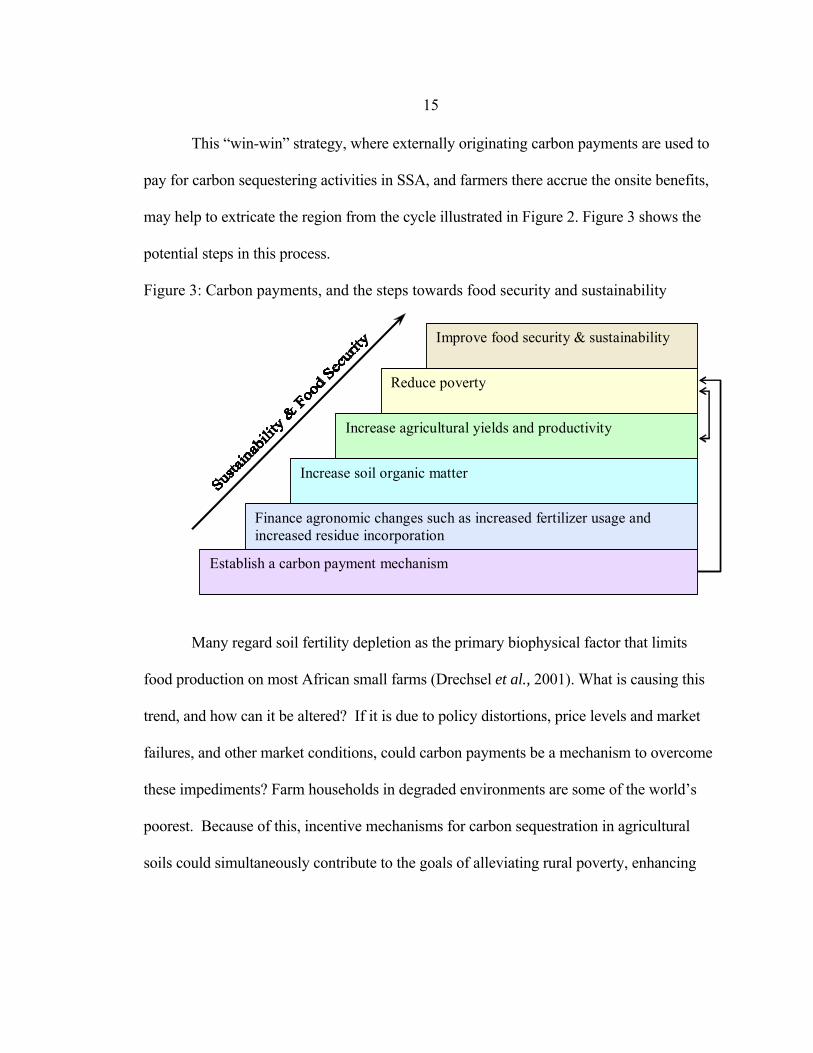
This “win-win” strategy, where externally originating carbon payments are used to
pay for carbon sequestering activities in SSA, and farmers there accrue the onsite benefits,
may help to extricate the region from the cycle illustrated in Figure 2. Figure 3 shows the
potential steps in this process.
Figure 3: Carbon payments, and the steps towards food security and sustainability
Finance agronomic changes such as increased fertilizer usage and increased residue incorporation
Establish a carbon payment mechanism
Increase soil organic matter
Increase agricultural yields and productivity
Reduce poverty
Improve food security & sustainability
Many regard soil fertility depletion as the primary biophysical factor that limits
food production on most African small farms (Drechsel et al., 2001). What is causing this
trend, and how can it be altered? If it is due to policy distortions, price levels and market
failures, and other market conditions, could carbon payments be a mechanism to overcome
these impediments? Farm households in degraded environments are some of the world’s
poorest. Because of this, incentive mechanisms for carbon sequestration in agricultural
soils could simultaneously contribute to the goals of alleviating rural poverty, enhancing

16
agricultural sustainability and mitigating greenhouse gas emissions (Soil Management
CRSP, 2002).
The use of agricultural soil carbon sequestration has been limited under the
Marrakesh Accords of the Kyoto Protocol (UNFCCC). The United States has not ratified
the Kyoto protocol, further limiting its role in policies to mitigate GHGs. The purpose of
this thesis is not to speculate about what role carbon sequestration may play under any
specific policy regime. Instead, this thesis will asses the role that soil carbon sequestration
might play in helping developing countries deal with soil degradation, if and when
governmental, non governmental or corporate entities take actions to reduce GHG
emissions.
Thesis Objectives
Human induced soil degradation has multiple forms, including: nutrient decline,
erosion, salinization and physical compaction (ISRIC GLASOD, 2004). In Sudo-Sahelian
Africa, erosion and nutrient mining are prominent causes of soil degradation. Nutrient
mining occurs when more nutrients, such as nitrogen, phosphorus, potassium, carbon, and
other micronutrients, are removed from the soil than are put back into the system. In the
case of Senegal, harvesting grains and crop residue from the land impact heavily on soil
carbon content, while insufficient replacement of soil nutrients with fertilizers leads to
negative nutrient balances. Policies that encourage or enable farmers to incorporate crop
residues into their soils, and to increase mineral fertilizer usage, would help to reduce or
reverse these types of soil degradation in the region.

17
Given the economic perspective of the rational farmer, and the dynamic nature of
crop and soil management issues, this thesis uses a regional case study in the Groundnut
Basin of Senegal to do the following:
• To describe and assess the economic incentives facing farmers specific to
the case study region. This study will examine institutions and conditions
that impact farmers' decisions.
• To model the farmer's production and decision making process.
• To design carbon contract policies and model them within the farmer’s
decision making process.
• To simulate the interaction between the current agricultural marketplace,
and the new carbon policies.
• To assess the role that carbon sequestration could play in helping the region
deal with soil degradation problems, if and when international action is
taken to reduce GHG emissions.
18
CHAPTER 2
THE FARMER AND THE CARBON CONTRACT
Nutrient Mining, and the Role of Fertilizer and Crop Residues in Agricultural Systems
Nutrient mining, a form of human-induced soil degradation, is prevalent
throughout Africa, including the Sudo-Sahelian region. Drechsel et al. (2001) define
nutrient mining as:
"…the net loss of plant nutrients from the soil or production system due
to higher nutrient outputs (through leaching, erosion, crop harvest, etc.)
than inputs (e.g. through rainfall, manure, mineral fertilizer, fallow),
resulting in a negative nutrient balance."
As described in Chapter 1, the majority of Sub Saharan Africa's soils are innately
poor. Most of the region's farmers operated in shifting cultivation systems until the mid
1900's. Until then, soil nutrient balance was largely maintained by a system that
interspersed crops with long periods of fallow. With population growth and
extensification, permanent cultivation replaced fallow systems, and the nutrient
equilibriums of those systems were upset. Without the use of fallows or other
management practices that would add organic matter and nutrients to soils, soil organic
carbon stocks will inevitably decline, often to less than 50 percent of natural conditions,
in several years (Koning and Smaling, 2005).

19
Throughout the Sahel, organic matter and nutrients are removed by harvesting
grains and by selling or burning the crop residues. While some processes, including
organic fertilizer application, atmospheric deposition, and biological fixation of nitrogen,
partially offset withdrawals from the system, they are not sufficient to sustain nutrient
balances. Stoorvogel and Smaling (1990, 2000) found that nutrient balances throughout
Sub Saharan Africa, including Senegal and other Sahelian Countries, were predominantly
negative. Multiple authors, including Joa and Kang (1989), Batiano et al.(1998), and
Swift et al. (1994), concur that a combination of mineral fertilizers, manure, and crop
residues need to be incorporated to maintain or improve crop production (Koning and
Smaling, 2005).
One reason for negative nutrient balances in Sub-Saharan Africa is that farmers
use very low quantities of fertilizer relative to other agricultural regions. Average
fertilizer use in SSA has been estimated at less than 15 kg per hectare as of 1994/95,
compared to more than 200 kg in East Asia, 125 kg for Asia as a whole and 65 kg in
Latin America (UNDP/UNECA Report in Diagana, 2003). Some farmers use no mineral
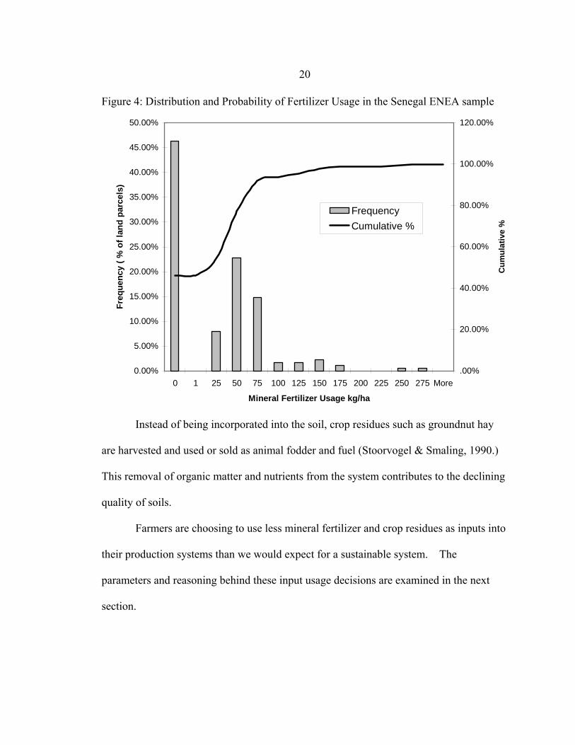
fertilizer at all in a given year. Figure 4 shows fertilizer usage distribution among the
Senegalese small holdings farmers used in the case study discussed in Chapter 4. This
figure shows that about 46 percent of parcels had no mineral fertilizer applied, and that
many who did apply fertilizer used relatively low rates.
20
Figure 4: Distribution and Probability of Fertilizer Usage in the Senegal ENEA sample
0.00%
5.00%
10.00%
15.00%
20.00%
25.00%
30.00%
35.00%
40.00%
45.00%
50.00%
0 1 25 50 75 100 125 150 175 200 225 250 275 More
Mineral Fertilizer Usage kg/ha
Freq
uenc
y ( %
of l
and
parc
els)
.00%
20.00%
40.00%
60.00%
80.00%
100.00%
120.00%
Cum
ulat
ive
%
FrequencyCumulative %
Instead of being incorporated into the soil, crop residues such as groundnut hay
are harvested and used or sold as animal fodder and fuel (Stoorvogel & Smaling, 1990.)
This removal of organic matter and nutrients from the system contributes to the declining
quality of soils.
Farmers are choosing to use less mineral fertilizer and crop residues as inputs into
their production systems than we would expect for a sustainable system. The
parameters and reasoning behind these input usage decisions are examined in the next
section.
21
Input Usage & the Rational Farmer
When farmers apply fertilizer or incorporate crop residue back into the soil, there
is a multi-period stream of benefits and costs associated with these practices. According
to economic theory, rational, risk-neutral farmers use mineral fertilizer such that VMPi =
wi, subject to spatial and temporal availability constraints. Where there are dynamic
effects of fertilizer and crop residue on SOC, the VMP can be interpreted as capturing all
(discounted) future productivity effects. In the absence of market distortions, farmers are
using fertilizer where their marginal benefit equals marginal cost (VMPi=wi). However,
distortions caused by poor infrastructure, import taxes , lack of capital markets for
wholesale and retail sectors, imperfect competition, and parastatal bureaucratic
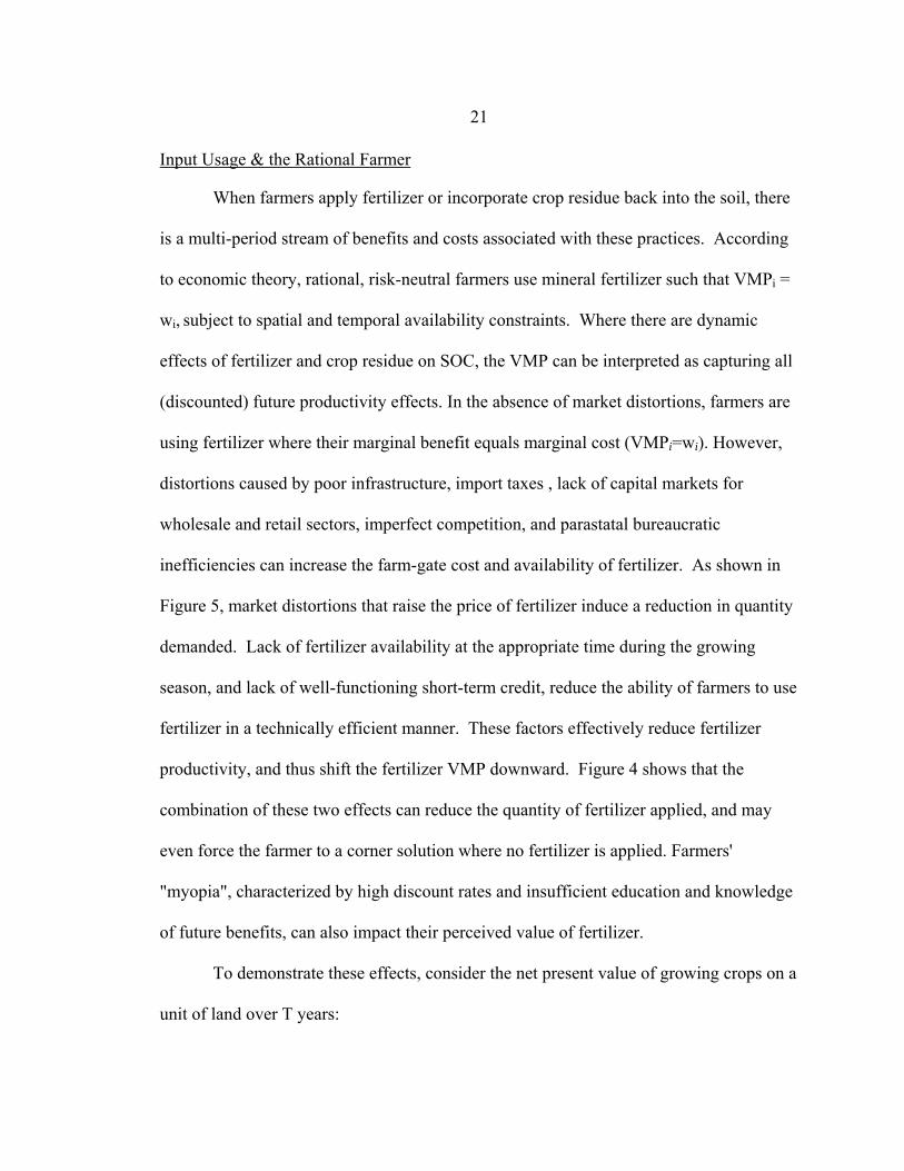
inefficiencies can increase the farm-gate cost and availability of fertilizer. As shown in
Figure 5, market distortions that raise the price of fertilizer induce a reduction in quantity
demanded. Lack of fertilizer availability at the appropriate time during the growing
season, and lack of well-functioning short-term credit, reduce the ability of farmers to use
fertilizer in a technically efficient manner. These factors effectively reduce fertilizer
productivity, and thus shift the fertilizer VMP downward. Figure 4 shows that the
combination of these two effects can reduce the quantity of fertilizer applied, and may
even force the farmer to a corner solution where no fertilizer is applied. Farmers'
"myopia", characterized by high discount rates and insufficient education and knowledge
of future benefits, can also impact their perceived value of fertilizer.
To demonstrate these effects, consider the net present value of growing crops on a
unit of land over T years:

22
(1) -1 -21
[ ( , ( , ,...)) - ]T
t t t t t t tt
NPV D p f x C x x w x=
= ∑
where Dt = (1/1+r)t, r is the interest rate, p and w are output and input prices, x is the
quantity of fertilizer, and C(.) is the stock of carbon which depends on past fertilizer
applications. Differentiating with respect to x1, the first-order condition for fertilizer use
in period 1 is:
1 1 1 12 1
T
t tt t
t t
f Cp f x D p wC x=
∂ ∂∂ ∂ + =
∂ ∂∑
The expression on the left-hand side is the value of the marginal product of fertilizer,
composed of the usual terms (price times marginal product) plus the discounted value of
the future impacts on productivity through carbon accumulation. As r increases, the
future stream of VMP, beyond year t, diminishes. As a result, the perceived VMP drops
as r rises, and farmers use less of the input.
Figure 5 shows how shifts in the VMP and in fertilizer markets can lower or
eliminate fertilizer usage. If the VMP of fertilizer is significantly suppressed by low
output prices or other factors discussed above, then a farmer that would have used F0
fertilizer with w0and VMP0 will instead use no fertilizer (F") in the VMP" case.
Similarly, where VMP=VMP0 if farm gate fertilizer prices are higher than w0, then
farmers would reduce fertilizer usage to F'b or F'a kilograms per hectare.
23
Figure 5: Fertilizer usage with market distortions
VMP''
kg fertilizer F'a,0 F0
w0
$/kg
w'a
Effect 1: higher input cost
F''
Effect 2: lower marginal productivity
VMP0
F'b
w'b
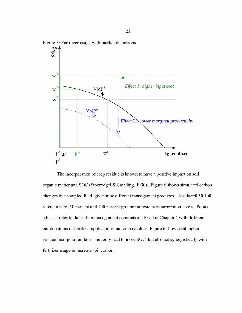
The incorporation of crop residue is known to have a positive impact on soil
organic matter and SOC (Stoorvogel & Smalling, 1990). Figure 6 shows simulated carbon
changes in a sampled field, given nine different management practices. Residue=0,50,100
refers to zero, 50 percent and 100 percent groundnut residue incorporation levels. Points
a,b,…, i refer to the carbon management contracts analyzed in Chapter 5 with different
combinations of fertilizer applications and crop residues. Figure 6 shows that higher
residue incorporation levels not only lead to more SOC, but also act synergistically with
fertilizer usage to increase soil carbon.

24
Figure 6: Average annual changes in SOC with carbon contracts on a sample field (Generated by the DSSAT/CENTURY model; t=20 years)
(16.00)
(14.00)
(12.00)
(10.00)
(8.00)
(6.00)
(4.00)
(2.00)
-
2.00
4.00
0 10 20 30 40 50 60 70
Annual Average Fertilizer kg/Ha
Ann
ual A
vera
ge ∆
Car
bon
(ton
nes/
ha)
Residue=100
Residue=50
Residue=0
g
d
i
h
cba = base practice
fe
In Senegal, there is a market for groundnut residue (hay) for livestock fodder, and it
is also valued for on-farm feed. If farmers incorporated residue, they would face these
opportunity costs, in addition to higher labor costs. As with fertilizer, farmers' high
discount rates lead to short time horizons, and undervaluing SOC maintenance. Farmers'
short-run VMP would be perceived as lower than it would be if they took into account the
long-term productivity effects. For this reason, and because relatively strong livestock
markets lead to high opportunity costs, residue incorporation is not common (if existent) in
the region of study.

25
Dynamics, Adoption Thresholds and the Role of Incentives
In this section, we consider farmers' decisions to adopt management practices that
sequester carbon (or slow the rate of carbon loss) in the soil. This analysis framework was
developed by Antle et al. (2001) and Antle and Diagana (2004).
To increase soil carbon stocks, a farmer must change from a given long-term
rotation system, i, (the historical land use baseline), and choose to adapt some carbon-
intensive land use system, k. We assume management practice i is used up to time 0,
resulting in soil carbon level Ci. The adoption of practice s at time 0 will cause Ci to rise to
Ck at time T. At this time T, soil carbon levels reach a new equilibrium level (referred to as
the "attainable maximum" by Ingram and Fernandes), until further management practice
changes occur. Literature (Watson et al., 2000) suggests that the path from Ci to Ck is
approximately linear over the time interval when most of the carbon is accumulated.
As discussed in Chapter 1, changes in management practices may have other
productivity inducing benefits beyond soil carbon accumulation, which can include
improvements in soil structure, water holding capacity, cation exchange capacity, and
increased topsoil depth. These other benefits, however, tend to occur after some time lag.
The magnitude of these long-term productivity effects, as well as farmers' discount rates
and financial positions, play crucial roles in the profitability of conservation investments
(Valdivia, 2002).
Carbon sequestration contracts could provide an additional financial incentive to
adapt these new management practices. Two types of carbon contracts are discussed in the
literature: per hectare contracts, where farmers are paid $gt dollars for each hectare on
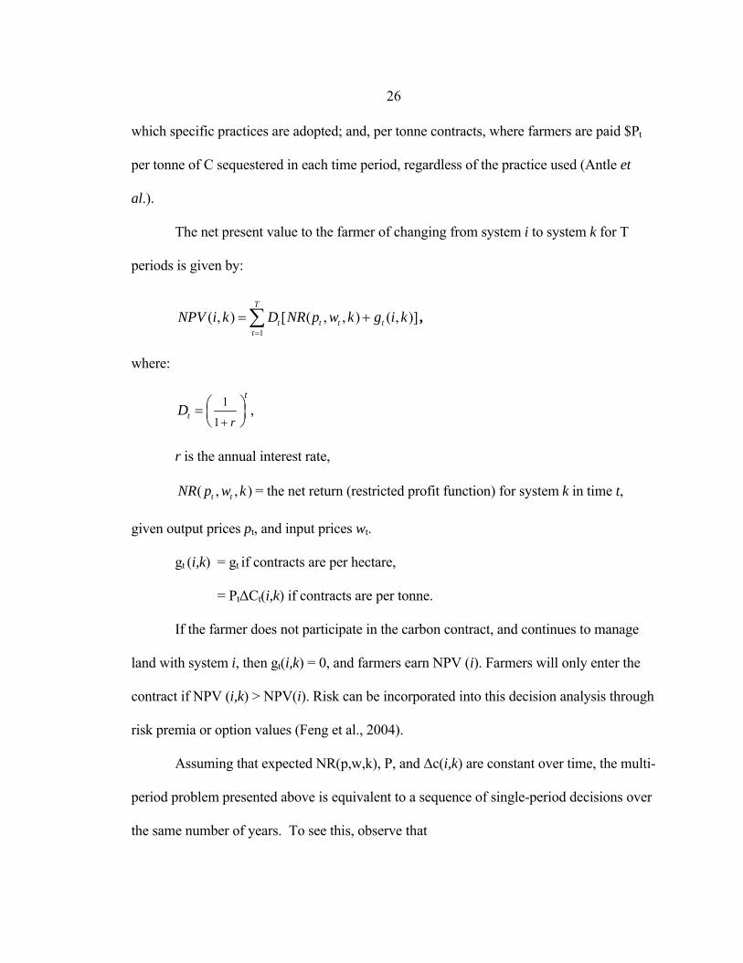
26
which specific practices are adopted; and, per tonne contracts, where farmers are paid $Pt
per tonne of C sequestered in each time period, regardless of the practice used (Antle et
al.).
The net present value to the farmer of changing from system i to system k for T
periods is given by:
1( , ) [ ( , , ) ( , )]
T
t t t tt
NPV i k D NR p w k g i k=
= +∑ ,
where:
1
1t
t
rD
+⎛ ⎞= ⎜ ⎟⎝ ⎠
,
r is the annual interest rate,
( , , )t tNR p w k = the net return (restricted profit function) for system k in time t,
given output prices pt, and input prices wt.
gt (i,k) = gt if contracts are per hectare,
= Pt∆Ct(i,k) if contracts are per tonne.
If the farmer does not participate in the carbon contract, and continues to manage
land with system i, then gt(i,k) = 0, and farmers earn NPV (i). Farmers will only enter the
contract if NPV (i,k) > NPV(i). Risk can be incorporated into this decision analysis through
risk premia or option values (Feng et al., 2004).
Assuming that expected NR(p,w,k), P, and ∆c(i,k) are constant over time, the multi-
period problem presented above is equivalent to a sequence of single-period decisions over
the same number of years. To see this, observe that
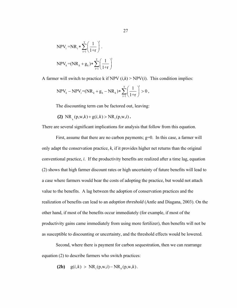
27
tT
i t=1
1NPV =NR1+ri
⎛ ⎞∗ ⎜ ⎟⎝ ⎠
∑ .
tT
t=1
1NPV =(NR g )1+rk k k
⎛ ⎞+ ∗ ⎜ ⎟⎝ ⎠
∑
A farmer will switch to practice k if NPV (i,k) > NPV(i). This condition implies: tT
t=1
1NPV NPV =(NR g NR ) 01+rk i k k k
⎛ ⎞− + − ∗ >⎜ ⎟⎝ ⎠
∑ ,
The discounting term can be factored out, leaving:
(2) NR (p,w, ) g( , ) NR (p,w, )k ik i k i+ > .
There are several significant implications for analysis that follow from this equation.
First, assume that there are no carbon payments; g=0. In this case, a farmer will
only adapt the conservation practice, k, if it provides higher net returns than the original
conventional practice, i. If the productivity benefits are realized after a time lag, equation
(2) shows that high farmer discount rates or high uncertainty of future benefits will lead to
a case where farmers would bear the costs of adopting the practice, but would not attach
value to the benefits. A lag between the adoption of conservation practices and the
realization of benefits can lead to an adoption threshold (Antle and Diagana, 2003). On the
other hand, if most of the benefits occur immediately (for example, if most of the
productivity gains came immediately from using more fertilizer), then benefits will not be
as susceptible to discounting or uncertainty, and the threshold effects would be lowered.
Second, where there is payment for carbon sequestration, then we can rearrange
equation (2) to describe farmers who switch practices:
(2b) g( , ) NR (p,w, ) NR (p,w, )i ki k i k> − .

28
The right hand side of this expression is the farmer's opportunity cost for switching from
system i to system k. The farmer will switch to practice k when the opportunity cost is less
than the payment per period. For per tonne contracts, g(i,k)= P∆c(i,k), and the participation
in these contracts can be expressed as:
(3)
NR(p,w, ) NR(p,w, )Pc( , )
i ki s
−>
∆ .
The right hand side of equation (3) is the farmer's opportunity cost per tonne of carbon.
The farmer will participate when the price per-tonne C is higher than the farmer's
opportunity cost per tonne C. In this case, the market price for carbon plays a pivotal role
in farmers' decisions to participate (Antle and Diagana, 2003).
Significantly, equation (3) demonstrates that when carbon payments are made, it
may be no longer necessary for the conservation practice to be privately more profitable
than the conventional practices. In cases where rational farmers are apprised of the benefits
of conservation practices, but they still do not adopt them, it is safe to assume that these
practices are not as profitable as the conventional ones. In these cases, additional positive
financial incentives are necessary to induce and maintain adoption.
Carbon Contracts for Fertilizer and Residue Incorporation
In this analysis per-tonne carbon contracts will be issued for adoption of carbon-
intensive management practices. Most of these possible contract scenarios will stipulate
minimum levels of mineral fertilizer usage, in concert with some level of crop residue
incorporation. On the whole, these contracts will encourage increased usage of mineral

29
fertilizer, which many West African farmers use at levels far lower than the rest of the
world. Long-term effects, such as carbon sequestration and those associated with increased
soil organic carbon are significant and dynamic; however, they are small in comparison to
the immediate short run productivity benefits of the increased fertilizer.
Figure 7 shows the net revenues, opportunity costs, and offset values required to
increase fertilizer usage. In this case, market distortions and conditions cause the VMP and
cost of using fertilizer to be VMP' and w', respectively. The profit function associated
with these conditions is NR'. Farmers are profit maximizers, and will use demand F' kg of
fertilizer per hectare.
Now, carbon contracts are offered to farmers, where, to fulfill these contracts, they
must switch from their current management practices, i, to a carbon-intensive management
system, k. This entails using fertilizer (and or residue) at rate F0, which is greater than F'.
There are two ways that this can be achieved. First, carbon payments can offset the
opportunity cost of changing practices, as shown in the top panel of Figure 7. From
equation (2b), the carbon payment, g, must be > (max NR' - NR^) for farmers to switch
practices.

30
Figure 7: Net revenue and opportunity costs associated with fertilizer usage
kg fertilizer0 F0
w 0
$/kg
w 'a
VMP0
F'
w ' VMP'
kg fertilizer0
NR^
NR $
max NR0
F0 F'
NR'
max NR'
NR0
opportunity cost

31
Carbon contracts may also increase fertilizer (and / or residue) inputs by offsetting
distortions and constraints in the input markets. If large-scale providers of carbon contracts
could provide fertilizer at lower cost to farmers, and provide it in a timely manner, it is
possible that farmers would use fertilizer at rate F0 because it would be cheaper and more
productive. In this case, farmers would be willing to enter carbon contracts simply to
obtain access to fertilizer. In this case, carbon payments do not need to be positive to spur
adoption of new practices because the opportunity cost of switching to the carbon-intensive
practice is negative.
When there are profitable uses of crop residues as feed or fuel, residue
incorporation carries a high price relative to the short-term agronomic benefits. In addition,
if farmers have high discount rates, or do not have access to credit markets, they will tend
to discount future benefits and thus will be likely to incorporate little if any residues into
the soil. If a carbon payment was used to promote residue incorporation (in concert with
fertilizer intensification), participating farmers would eventually capture the long-term
agronomic benefits of the practices, which would eventually increase the profitability of the
carbon-intensive management practices. An important empirical question is how large of
an incentive would be required to induce farmers to incorporate enough crop residues to
reduce or reverse the loss of SOC.
It is likely that a combination of carbon payments and market distortion offsetting
can be used to increase carbon intensive management practices. In simulation, we expect
that if the contracts simply make fertilizer temporally available to farmers, that some
farmers will join the contracts and switch practices, even without a carbon payment. This

32
would support the hypothesis that fertilizer availability is binding. We also expect, as
carbon payments increase, more and more farmers will switch practices, and would
increase the supply of carbon sequestration services.
In this analysis, we attempt to anticipate some of the possible farmer incentives
associated with participating in carbon contracts, and the likely ability of each policy to
induce farmers to undertake new management practices. While acknowledging the
importance of transaction cost and permanence issues, this thesis aims to establish the
economic potential of carbon sequestration, abstracting from these issues. We leave these
problems to future work.
33
CHAPTER 3
THE SIMULATION APPROACH
Modeling Complex Systems
The scientific community recognizes that many economic, environmental and other
biophysical phenomena are best described as complex systems. Biophysical models have
been applied to agricultural production systems to model a restricted set of properties,
including; crop growth (Whisler et al., Ritchie), hydrologic transport and cycling (e.g., de
Willigen et al., Ghardiri and Rose), soil OM and nutrient dynamics (Paustian, Powlson et
al.), and crop-livestock production systems (Thornton and Herrero) (Antle and Capalbo,
2002). Larger biogeochemical models, which incorporate all or most pertinent subsystems,
characteristically focus on the dynamics of the nutrients, biomass and carbon within an
ecosystem (e.g. Hunt et al., Parton et al). Ecological processes, such as primary
consumption, production, decomposition and energy transfers are concatenated at different
temporal and spatial scales with mechanistic and empirical formulations. In these cases,
however, human behavior and decisions are treated as exogenous, and their economic
behavior is “conceptually outside the boundaries of the system” (Antle and Capalbo, 2002).
In the same way, boundary conditions or constraining variables in biophysical
models are often endogenous to a system, yet economists typically take these biophysical
variables as exogenous or represent them with simple empirical relationships (Antle and

34
Capalbo, 2002). Mathematical programming and econometric production models have
been linked with biophysical models3, usually by taking the output from one model (e.g. an
input use decision for an economic model, or yield from a crop growth model), and using it
as the input into another model.
Integrated Assessment for Agricultural Production Systems_______________
Antle and Capalbo (2001) described the integrated assessment paradigm for
agricultural production systems. To paraphrase, soils and climate data are inputs into crop
and livestock process models, which calculate site and time specific productivity. Outputs
from the crop and livestock models, such as crop yield and livestock productivity, may then
be inputs into economic models. Outputs from these crop and livestock model, and
economic data are also used as inputs into economic production models. Outcomes of both
of these model types (crop yield, livestock productivity, and land and input use decisions)
may then be incorporated into environmental process models, which could model processes
such as chemical leaching, and soil erosion. Assuming that the biophysical and economic
data are representative of the land units and decision makers in a population, these models
can then be used to aggregate environmental and economic outcomes for a region,
demonstrating tradeoffs for policy makers within the region.
This multidisciplinary approach can be modeled with software that integrates the
economic and biophysical models. In this case the Tradeoff Analysis Model and Software,
version 3.1, will be used (Stoorvogel et al., 2001).
3 See Antle and Capalbo for a review of this literature.
35
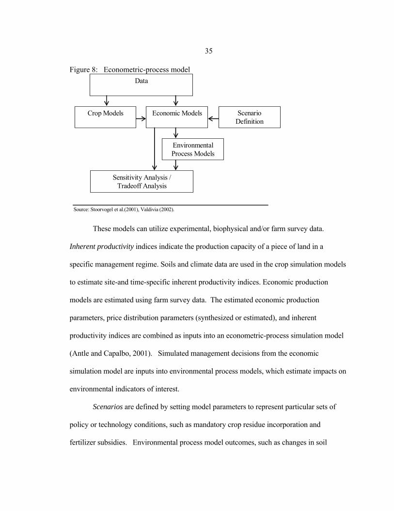
Figure 8: Econometric-process model Data
Economic Models
Sensitivity Analysis / Tradeoff Analysis
Environmental Process Models
Scenario Definition
Crop Models
Source: Stoorvogel et al.(2001), Valdivia (2002).
These models can utilize experimental, biophysical and/or farm survey data.
Inherent productivity indices indicate the production capacity of a piece of land in a
specific management regime. Soils and climate data are used in the crop simulation models
to estimate site-and time-specific inherent productivity indices. Economic production
models are estimated using farm survey data. The estimated economic production
parameters, price distribution parameters (synthesized or estimated), and inherent
productivity indices are combined as inputs into an econometric-process simulation model
(Antle and Capalbo, 2001). Simulated management decisions from the economic
simulation model are inputs into environmental process models, which estimate impacts on
environmental indicators of interest.
Scenarios are defined by setting model parameters to represent particular sets of
policy or technology conditions, such as mandatory crop residue incorporation and
fertilizer subsidies. Environmental process model outcomes, such as changes in soil
36
carbon, and predicted land use decisions and economic markers, such as tenure choice and
net returns, can be aggregated to assess the environmental and economic impacts of each
policy. Using the Tradeoff Analysis software, a set of parameters can be varied while
holding others constant to conduct sensitivity analysis.
Methods
This sub-section contains a description of the relationship between economic and
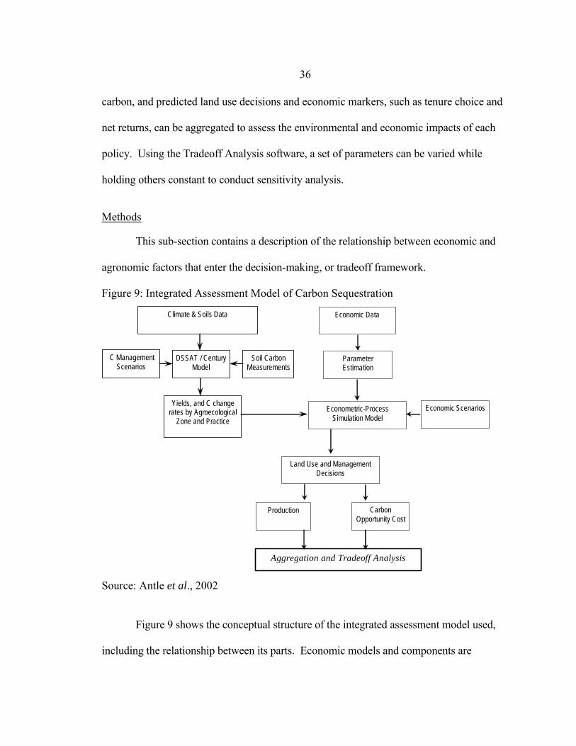
agronomic factors that enter the decision-making, or tradeoff framework.
Figure 9: Integrated Assessment Model of Carbon Sequestration
Parameter Estimation
Economic Data
Econometric-Process Simulation Model
Land Use and Management Decisions
Production Carbon Opportunity Cost
Aggregation and Tradeoff Analysis
Soil Carbon Measurements
Climate & Soils Data
Yields, and C change rates by Agroecological
Zone and Practice
DSSAT / Century Model
C Management Scenarios
Economic Scenarios
Source: Antle et al., 2002
Figure 9 shows the conceptual structure of the integrated assessment model used,
including the relationship between its parts. Economic models and components are

37
depicted on the right side of the figure, while agronomic, soils, and environmental models
are on the left.
Crop and Carbon Models
DSSAT/CENTURY. The DSSAT/CENTURY model (Gijsman et al., 2002) was
used by a collaborating team of scientists to estimate soil carbon changes and inherent
productivity for conditions representing each village in this study. The DSSAT/CENTURY
model was developed by linking the DSSAT crop modeling system to the CENTURY
model’s method of simulating soil carbon dynamics. The DSSAT/CENTURY model was
developed specifically for low input systems where most nutrients become available from
soil organic matter (SOM) and residue turnover. The DSSAT/CENTURY model estimates
changes in soil organic carbon stocks, using variables such as crop type, tillage mechanism,
fertilizer usage, residue incorporation and rainfall. Using the model, initial and final values
of soil carbon and crop yields were determined for each field, over a pre-determined time
period (in this case, twenty years). The model was implemented using soils and climate
data for the region and parameters for groundnut and millet crops from the region. The
model was simulated for representative soil and climate conditions in each village
represented in the study.
Modeling Changes in Inherent Productivity and Soil Carbon Stocks. The inherent
productivity attributed to a field in any year, t, is:
20 00
0 20 20
( )t
t
inprod inprodinprod inprod t
≤ ≤
−= + × .
38
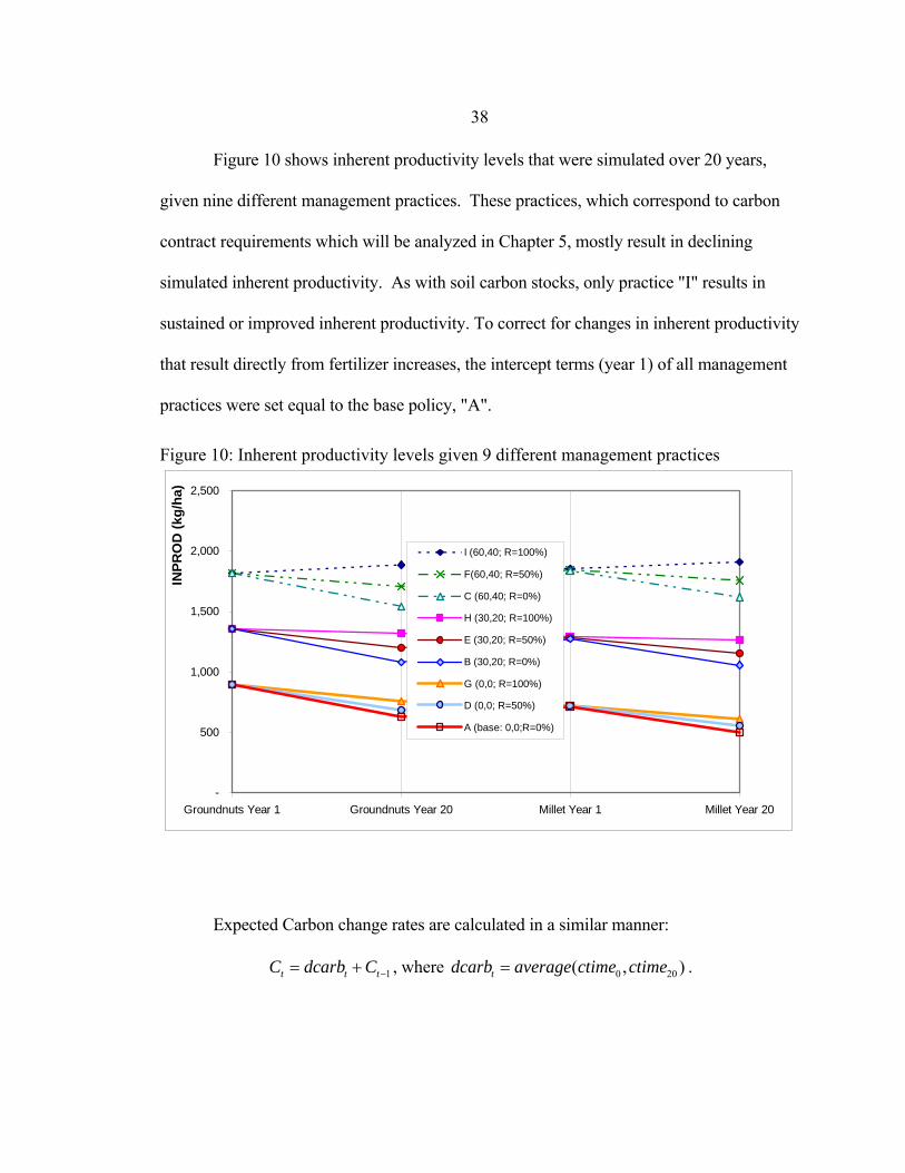
Figure 10 shows inherent productivity levels that were simulated over 20 years,
given nine different management practices. These practices, which correspond to carbon
contract requirements which will be analyzed in Chapter 5, mostly result in declining
simulated inherent productivity. As with soil carbon stocks, only practice "I" results in
sustained or improved inherent productivity. To correct for changes in inherent productivity
that result directly from fertilizer increases, the intercept terms (year 1) of all management
practices were set equal to the base policy, "A".
Figure 10: Inherent productivity levels given 9 different management practices
-
500
1,000
1,500
2,000
2,500
Groundnuts Year 1 Groundnuts Year 20 Millet Year 1 Millet Year 20
INPR
OD
(kg/
ha)
I (60,40; R=100%)
F(60,40; R=50%)
C (60,40; R=0%)
H (30,20; R=100%)
E (30,20; R=50%)
B (30,20; R=0%)
G (0,0; R=100%)
D (0,0; R=50%)
A (base: 0,0;R=0%)
Expected Carbon change rates are calculated in a similar manner:
1t t tC dcarb C −= + , where 0 20( , )tdcarb average ctime ctime= .

39
Figure 11 shows potential paths of carbon sequestration for a field, given two land
management practices, a and b. Path “a” shows the relative carbon change path of the field
if management “a” was adapted in year one, and used continually for twenty years. Path
“a2” shows the decision to follow management “a” for fourteen years, and then switch to
policy “b”. Similarly, path “b” depicts exclusive use of management “b”, while b2 depicts
the relative carbon change path of implementing management “b” for nine years, and then
switching to “a.” Unlike the inherent productivity numbers, all management practices start
with the same value, so no intercept correction was needed for this simulated variable (see
Figure 1 on page 13).
Figure 11: Time Paths of Carbon Changes in a Field
t
Exp
ecte
d C
arbo
n C
hang
e R
elat
ive
to B
ase
Prac
tice
10 20
b2
a2
dCt=20, policy b
t=0
dCt=20, policy a
b
α
φ
a
Two major simplifying assumptions are made here; first, expected soil carbon
increases or decreases linearly; and second, it increases or decreases at the same rate,
regardless of initial level. For example, it assumes that soil carbon decreases at the same
linear rate if a farmer used policy “b” from year 0, versus starting at point α in year 14.

40
Economic Models: The Econometric Process Simulation Model________
Antle and Capalbo (2001) developed the econometric process simulation model,
which merges econometric production models, represented by supply and demand
equations with discrete process-based land use decisions, represented by the threshold
equation for contract participation, Equation (3).
In the econometric process simulation model, parameters and state variables are
estimated in the biophysical and economic models, and those estimates are then used in
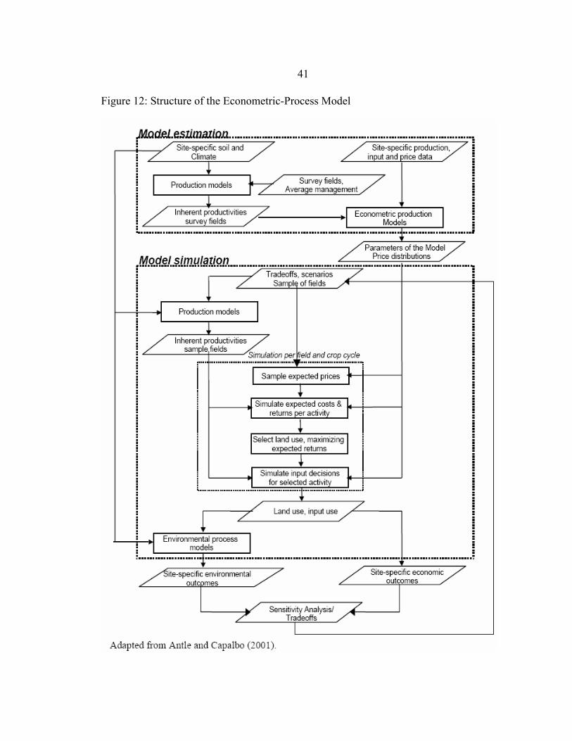
simulation to predict discrete land use decisions for each field in each year. Figure 12
depicts the structure of the econometric process simulation model, with the upper half
representing the estimation steps of the econometric models, and the lower part
representing the simulation model structure. The latter model simulates the farmer’s land
use choice on a given field in a given year, and the related output and input usage
corresponding to that choice.
The output can be interpreted as a “statistical representation of the population of
land units in an agricultural region” (Antle and Capalbo, 2001) because of the stochastic
nature of the sample data and the econometric models. In addition to this, because the
simulation operates at the field scale using site-specific data, it can represent temporal and
spatial variations in land use over time. These variations, such as tenure system, and crop
rotations, can lead to different regional economic and biophysical outcomes over space and
time.
41
Figure 12: Structure of the Econometric-Process Model

42
Sensitivity Analysis of Soil Carbon Management Using Integrated Assessment Models
The General Approach. Agricultural systems are complex, dynamic systems, with
biophysical and economics variables and parameters. Particularly in developing countries,
the quality of data available to researchers can be less than perfect. This, in addition to
inherent or unforeseen fluctuations in a system, can generate uncertainty in a model.
Changes in parameters and exogenous variables can affect model outcomes (Valdivia,
2002).
Influences on the reliability, efficiency and robustness of a model vary from
parameter to parameter. The appropriateness, or relevance, of a model highly depends on
the sensitivity of outcomes with respect to its parameters. Valdivia (2002) cites several
reasons to use analysis, including:
• Identifying critical thresholds, or values where the optimal strategy changes.
• Identifying sensitivity to important, changeable, variables.
• Testing the robustness of an optimal solution. This indicates the robustness
with regards to changes in key parameters, and speaks to the relevance of
those parameters and the model.
In an effort to understand the causal relationships within and between complex
systems, integrated analysis combines, interprets, and communicates knowledge from
diverse disciplines. Researchers have many tools for this approach, including computer-
aided modeling, scenario analyses, simulation and experience-and expertise-based
participatory integrated assessment (IPCC, 2001).

43
Comparisons of different models and model variants by the IPCC show that model
results are very sensitive to alternative climate model inputs, which explains the large
variance in yield estimates from crop models. Uncertainties in economic models alone are
substantial, implying that the "economic impacts of climate change on agriculture are given
a low degree of confidence" (Valdivia, 2002). As a result, integrated assessment and
econometric modelers need to use sensitivity analysis to identify key assumptions and
parameters, and focus research on those areas of the models. The scenario analysis
approach is used in this thesis to conduct sensitivity analyses of the model.
Scenario Analysis
The scenario analysis approach, also call parametric analysis, assumes scenarios by
specifying ranges and/or combinations of selected parameter values. The researcher solves
the problem repeatedly, obtains a range of solutions, and observes sensitivities. From this,
an approximation is chosen subjectively. Key parameters, distribution or range
specifications, and the assignment of specific values such as maximums, are usually also
obtained with this subjective method.
Scenarios are descriptions of possible future states that are described without
ascribed probabilities. While these scenarios may contain sources of uncertainty, they are
generally not explicitly acknowledged. Combinations of two or more scenarios can be
used to construct ranges of possible outcomes that are sensitive to these sources of
uncertainty.
The integrated simulation model applied in this thesis uses linked econometric and
biophysical models. It allows comparisons of tradeoffs between prevailing and future

44
economic and environmental outcomes. We conduct a sensitivity analysis with the
information produced by an integrated assessment model by varying important parameters,
including: input and output prices, yield responses, contract costs, and contract
requirements.
45
CHAPTER 4
CASE STUDY: SENEGAL
General work has been completed regarding factors impacting Carbon sequestration
in developing countries, however specific, “detailed case studies are needed to assess the
economic feasibility of soil Carbon sequestration under conditions representing different
parts of the world” (Antle & Diagana, 2003). This study will focus on the groundnut basin
of Senegal.
Geography
Senegal is located in the Atlantic Sahelian region of Sub Saharan Africa. Figure 13
depicts Senegal's location, and the Sahelian zone of Africa. Sub Saharan Africa is the
region south of the Sahara Desert, which includes all nations of the Sahel and southwards.
Most of Senegal's crop production is dryland, or un-irrigated. Senegal's national
crop composition is shown in Figure 14.

46
Figure 13: Map of Africa
S E N E GAL
Source: PERC, 2004, with Senegal emphasis by author
Figure 14: Crop Area in Senegal, 2001/2002 Crop Year
Crop Area 2001/2002total= 2,223,456 ha
Cotton1.4%
Maize4.0%
Rice(paddy)3.9%
Sugarcane0.3%
Manioc1.3%
Millet and Sorghum
43.9%
Groundnuts44.3%
Vegetables1.0%
Source: IMF, 2003

47
The Groundnut Basin of Senegal is dominated by millet and groundnut production.
Figure 15 shows the major agricultural zones of Senegal. This area represents roughly one
third of Senegal’s total landmass, and three quarters of its arable land (Kelly et. al., 1996;
Akobundu, 1998). Overall, the GB accounts for 80% of Senegal’s exportable groundnut
crop, and 70% of its national cereal crop. Of the total cultivated area in the Groundnut
Basin, groundnuts make up 50% of seeded acreage, followed by millet and sorghum (45%),
with the remainder planted in maize, cassava and cowpeas (Badiane, 2001).
The Groundnut Basin is comprised of the following regions; the Northern, Central,
and Southern Groundnut Basins, the Eastern Region and Casamance. Table 2 summarizes
the characteristics of these regions. In the literature, there is some variation in the
delineation and description of the different Groundnut Basin regions (Soufi, 2001). Overall,
however, it can be said that both rainfall and soil clay content increase as one moves from
North to South.
Figure 15: Map of Senegal, and Senegal’s Groundnut Basin
LEY
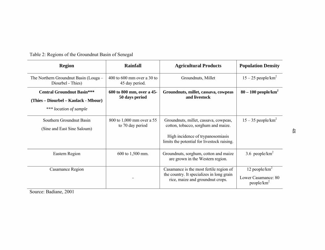
Table 2: Regions of the Groundnut Basin of Senegal
Region Rainfall Agricultural Products Population Density
The Northern Groundnut Basin (Louga – Diourbel - Thies)
400 to 600 mm over a 30 to 45 day period.
Groundnuts, Millet
15 – 25 people/km2
Central Groundnut Basin***
(Thies – Diourbel – Kaolack - Mbour)
*** location of sample
600 to 800 mm, over a 45-50 days period
Groundnuts, millet, cassava, cowpeas and livestock
80 – 100 people/km2
Southern Groundnut Basin
(Sine and East Sine Saloum)
800 to 1,000 mm over a 55 to 70 day period
Groundnuts, millet, cassava, cowpeas, cotton, tobacco, sorghum and maize.
High incidence of trypanosomiasis limits the potential for livestock raising.
15 – 35 people/km2
Eastern Region 600 to 1,500 mm. Groundnuts, sorghum, cotton and maize are grown in the Western region.
3.6 people/km2
Casamance Region
-
Casamance is the most fertile region of the country. It specializes in long grain
rice, maize and groundnut crops.
12 people/km2
Lower Casamance: 80 people/km2
Source: Badiane, 2001
48

49
Historical Background
Senegalese agriculture has changed substantially through the last century. The
policies of the colonial and independent governments, as well as those imposed by Bretton
Woods institutions are summarized in this section.
The Colonial Period. At the beginning of the 20th century, Senegal was a French
colony. Groundnut production was left to the peasants, while the Government tried to spur
economic development by investing in rail, road and harbour infrastructure development.
The transport of groundnuts was financed by French merchant companies who operated
with local, often Lebanese, agents. These agents also imported consumer goods and rice
for the farmers to purchase. In order to offset the rural food deficit, which was created by
farmers focusing groundnuts for export, and to supplement urban food needs, the colonial
Government encouraged importation of broken rice from French Indo-China. During this
period, credit was important to farmers, both for purchasing food during scarcity, and for
groundnut seed, which is required in high ratios relative to output. Low prices and
preparation ease soon made rice the preferred urban staple food and a significant millet
complement in rural households (Faye et al., 2001).
French colonial rule left Senegal highly dependant on groundnut export revenues.
For many years after Independence, Senegal's food strategy differed little from patterns
established during the colonial period. Specialization in producing and exporting groundnut

50
products to finance cereal importation was encouraged; and, there was substantial state
involvement in production and marketing (Akobundu, 1998).
Independence. In 1960, Senegal gained independence as a nation.
Demographically, there was a small, well educated urban elite who, because of the French
education system, had been largely differentiated from rural peoples (Wilson & Fall, 2000).
This elite and the political leadership were instilled with the prevailing socialist state
planning ideas of the time.
The new government’s Programme Agricole policies, which were in effect from
the 1960s to the 1980s, used co-operative parastatals to organize and handle Senegal's
farmers and their produce (Faye et al., 2001). In the 1960s, French firms were driven out of
intermediary roles, while the co-operative parastatals were slowly given monopolies in
domestic groundnut trade, farm inputs, rice and other cereals. As a result, farmers were
required to be members of these co-operatives. ONCAD (Office National de
Commercialisation et d'Assistance) was the large parastatal responsible for channeling
credit and inputs downwards and groundnuts upwards. French firms retained control of the
processing and exporting sectors. SATEC, which later became SODEVA (Société de
Développment et de Vulgarisation Agricole), provided training services to farmers who
were now using credit-provided animal-drawn equipment. With the Programme Agricole,
all prices were fixed by the state. Large margins were set between export prices and farm
gate prices, which financed the number of state employees, and increased the taxable
profits of downstream industries (Faye et al., 2001). Pricing was based on the principle of
paying farmers just enough to keep them producing groundnuts, but not enough for farm
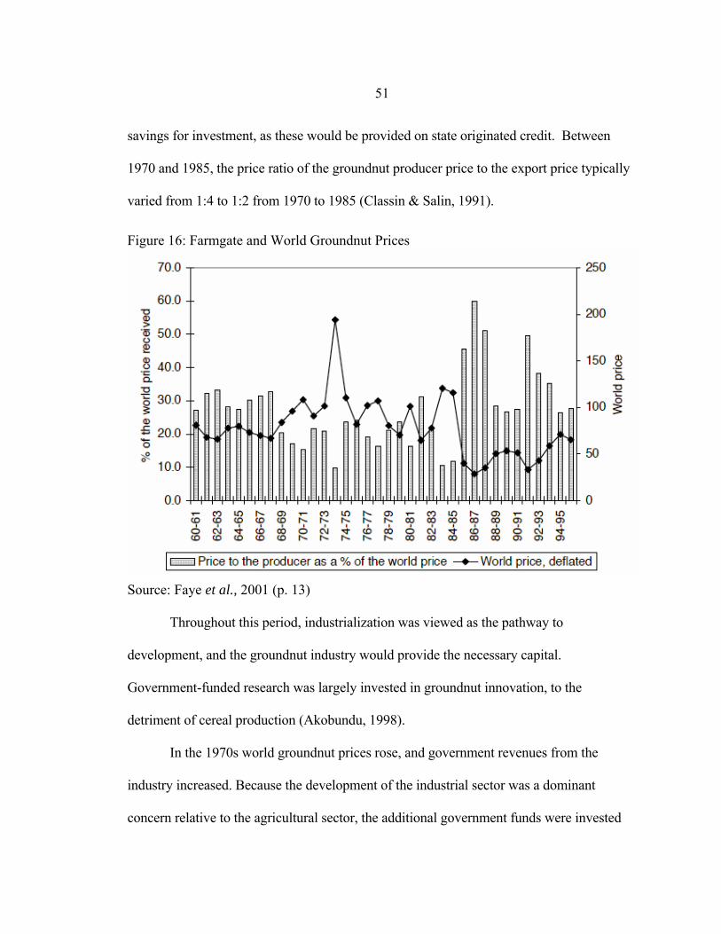
51
savings for investment, as these would be provided on state originated credit. Between
1970 and 1985, the price ratio of the groundnut producer price to the export price typically
varied from 1:4 to 1:2 from 1970 to 1985 (Classin & Salin, 1991).
Figure 16: Farmgate and World Groundnut Prices
Source: Faye et al., 2001 (p. 13)
Throughout this period, industrialization was viewed as the pathway to
development, and the groundnut industry would provide the necessary capital.
Government-funded research was largely invested in groundnut innovation, to the
detriment of cereal production (Akobundu, 1998).
In the 1970s world groundnut prices rose, and government revenues from the
industry increased. Because the development of the industrial sector was a dominant
concern relative to the agricultural sector, the additional government funds were invested

52
the industrial sector. This investment funded factories for textiles, phosphate fertilizer,
fishmeal, groundnut oil and feedcake.
When the economic boom of 1974 -1976 ended, groundnut prices returned to
approximately pre-1974 levels. Lower rainfall levels, from 1968 to the early 1970s
undermined farmer's production capacity, leaving many farmers unable to repay their credit
obligations. During that period, civil unrest led the Government to forgive farmer debt
three times. This, in addition to inefficiencies and corruption within ONCAD, led to huge
debts for that organization.
Structural Adjustment and Beyond. Senegal experienced a macroeconomic crisis
from the late 1970's to the early 1980's. Responding to this, Senegal agreed to undergo
structural adjustment measures imposed by the International Monetary Fund (IMF) and
World Bank. These adjustments, and the associated Nouveau Politique Agricole (NPA)
programs, took effect in 1985, and continued until 1994, when the currency, the Franc de
la Communauté Financière Africaine (FCFA or CFA Franc) was devalued. These drastic
reforms were aimed at using market forces to motivate farmer decisions - turning “peasants
into farmers”. ONCAD was abolished in 1980; some agricultural extension services were
phased out; large government fertilizer subsidies ended in 1984; and in 1985, credit supply
was halted (Faye et al., 2000). However, despite an overall trend towards less contribution,
the government was still involved in input markets, output markets, and in the setting of
price floors and ceilings for various crops.
In 1995, the Senegalese Government made a commitment to privatize the state-
owned groundnut enterprise, the Société Nationale de Commercialisation des Oléagineux
53
du Sénégal (SONACOS), although at the time no buyers could be found. The Societé
National de Graines de Semance du Sénégal (SONAGRAINES), which is a descendant of
the abolished input parastatal ONCAD, was downsized and transferred its seed
procurement functions to official cooperatives and licensed traders, but in reality, both of
these groups were “agents of SONACOS rather than independent and competing traders”
(Kherallah et.al., 2002). Today, SONACOS still handles most of the unshelled groundnut
and groundnut oil trade in Senegal, and is still state owned. Through SONACOS and
SONAGRAINES, the Government continues to control producer prices, and a large portion
of the marketing, processing and input supply channels to oil groundnuts in Senegal
(Kherallah et.al., 2002).
Crisis in Senegal
This section explores the perceived crisis in the natural resource based economies
of Senegal. It will cover the fall in production, the drought, demographic changes, the
elimination of subsidies, the fall in new land available for cultivation, and finally, the rise
of soil degradation
Falling Production. Between 1960-1970 and 1990-1996, there was a 28%
reduction in national groundnut production. This was due to both reduced acreage (19%
less) and lower yields (11% less). Over that same period of time, there was a slight
increase in millet production, but this was outstripped by population growth (Faye et al.,
2001). Figure 17 shows these trends for the Diourbel Region of the Groundnut Basin.

54
Besides minor changes in crop selection, these drops in production have been
attributed to “changes in rainfall and poor resource management and environmental
degradation leading to lower output, this being propelled by population growth and
pressure on the resource base” (Faye et al., 2001). However, economic factors such as
prices also contribute to decreased production.
Figure 17: Production of groundnuts and millet per capita (Diourbel Region), in tonnes
Source: Faye et.al., 2001, p. 6.
Drought in the Sahel. The entire Sahelian region, including the region of study, has
been subject to a prolonged drought. Figure 18 shows rainfall trends and levels in Senegal's
groundnut basin over the past 30 years. The Diourbel region has experienced substantial
demographic and climactic stresses (Mortimore et al., 2004). This area, in the Central and
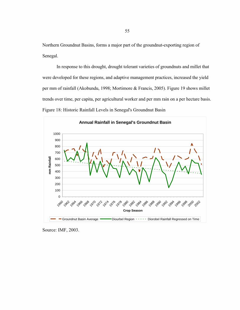
55
Northern Groundnut Basins, forms a major part of the groundnut-exporting region of
Senegal.
In response to this drought, drought tolerant varieties of groundnuts and millet that
were developed for these regions, and adaptive management practices, increased the yield
per mm of rainfall (Akobundu, 1998; Mortimore & Francis, 2005). Figure 19 shows millet
trends over time, per capita, per agricultural worker and per mm rain on a per hectare basis.
Figure 18: Historic Rainfall Levels in Senegal's Groundnut Basin
Annual Rainfall in Senegal's Groundnut Basin
0
100
200
300
400
500
600
700
800
900
1000
1960
1962
1964
1966
1968
1970
1972
1974
1976
1978
1980
1982
1984
1986
1988
1990
1992
1994
1996
1998
2000
2002
Crop Season
mm
Rai
nfal
l
Groundnut Basin Average Diourbel Region Diorobel Rainfall Regressed on Time
Source: IMF, 2003.
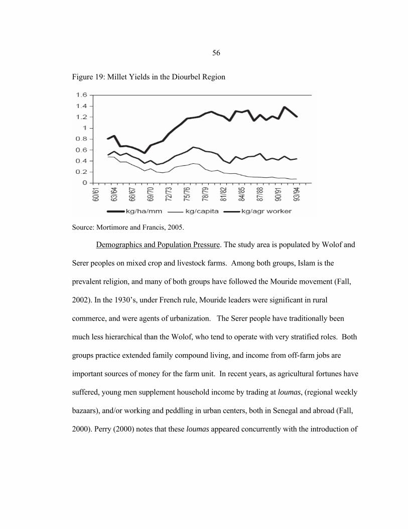
56
Figure 19: Millet Yields in the Diourbel Region
Source: Mortimore and Francis, 2005.
Demographics and Population Pressure. The study area is populated by Wolof and
Serer peoples on mixed crop and livestock farms. Among both groups, Islam is the
prevalent religion, and many of both groups have followed the Mouride movement (Fall,
2002). In the 1930’s, under French rule, Mouride leaders were significant in rural
commerce, and were agents of urbanization. The Serer people have traditionally been
much less hierarchical than the Wolof, who tend to operate with very stratified roles. Both
groups practice extended family compound living, and income from off-farm jobs are
important sources of money for the farm unit. In recent years, as agricultural fortunes have
suffered, young men supplement household income by trading at loumas, (regional weekly
bazaars), and/or working and peddling in urban centers, both in Senegal and abroad (Fall,
2000). Perry (2000) notes that these loumas appeared concurrently with the introduction of

57
structural adjustment policies in Senegal. The diminished importance of parastatals in the
rural marketplace gave rise to loumas as the local economic hubs.
This area has been subject to a high rate of population growth; the national growth
rate is 2.4% per annum (WHO, 2004), and regional rural growth estimates range from 2.8%
to 3.24% (Barry et al. 2000). People were living at variable densities of 46–151/km2 at the
time of the 1988 census (Barry et al., 2000). Fields are small (about .5 ha) with cereals
(mainly bulrush millet) grown for subsistence. Over 80% of the land has been under
cultivation or short, 1-year fallows since 1954 or earlier (Ba et al., 2000). In recent years,
fallow has dropped to very low levels (0.5-2%) in some areas, and has virtually
disappeared in others.
The Groundnut Basin is proximate to Dakar, population 2.6 million (World
Gazeteer, 2004). Between the Administrative Regions of Dakar, Diourbel, and Thiès,
there are over 5 million of Senegal’s 10 million people (see Table 3). This density not only
puts pressure on rural area for land cultivation, but it also creates a large demand center for
other regional resources and products.
Table 3: Population Statistics Admin Region
Population km2 persons/ km2
Dakar 2,613,700 550 4752 Diourbel 1,008,000 4,359 231
Thiès 1,461,700 6,601 221 3 Regions 5,083,400 11,510 442 Senegal 10,624,800 196,722 54
58
Price and Policy Roots of Production Decline. While population pressure and
drought have placed significant pressure on the agricultural systems of Senegal, production
has dropped for other reasons as well. Farmers, being rational, will adjust their
management practices, including input usage, based on the prices and information before
them.
Input Markets and Policies
During structural adjustment, once government fertilizer subsidies were eliminated,
prices rose, and in the absence of accompanying investments for physical and institutional
infrastructure to support markets, the availability of inputs decreased (Diagana, 2003). In
the Groundnut Basin,
"Fertilizer, agricultural equipment, seeds, and credit were all subjected to different
rules governing their supply and accessibility to farmers. Input supply policy
became as variable as the weather while the government sought the magic
combination of policies that would increase cereal production and involve the
private sector in the input and output marketing activities of the agricultural
sector."
(Akobundu, 1998, pp. 11-12)
Through this period, the documented lack of stability in policies pertaining to key
inputs was a likely cause of decreased input use, and therefore decreased production. In
response to the decreased fertilizer use, USAID/Senegal subsidized private sector fertilizer
purchases by farmers from 1986 through 1989 on a declining basis (Kelly et al., 1996).
Despite this effort, overall fertilizer usage did not recover to earlier levels, as farmers did

59
not have access to adequate credit markets to finance the private market purchases. When
the CFA Franc was devalued in 1994, fertilizer became relatively more expensive, which
again discouraged its use. Today, farmers still face liquidity constraints when buying
fertilizer, as payments for government purchased groundnuts (via SONACOS) are not
always made in time to purchase fertilizer for the next growing season.
Figure 20: Fertilizer Subsidy Rate in Senegal (% of full cost)
0102030405060708090
1975
1976
1977
1978
1979
1980
1981
1982
1983
1984
1985
1986
1987
1988
1989
1990
Data Source: (Kherallah et.al., 2000).
As discussed above, the policy changes associated with structural adjustment
adversely affected input usage. In the case of fertilizer, subsidies have been eliminated, and
private companies have not been fully able to fill the gaps efficiently. In combination with
these higher fertilizer prices, there is evidence that government involvement in output
markets suppresses output prices (see Figure 16). Figure 21 shows the relationship
between fertilizer and output prices over time. As this ratio increases, farmers will use less
and less fertilizer.

60
Other input markets have also been affected by policy changes. SONAGRAINES
and its predecessors used to provide funding for extension and research services, as well as
subsidies and credit services for certified groundnut seed. As the government has reduced
and eliminated these services, this has also lead to decreased potential returns to fertilizer
application. Also, given limited budgets and lack of credit, farmers tend to substitute
higher seeding densities for fertilizer usage (Kelly et al., 1996).
Figure 21: Kilograms of groundnuts necessary to purchase 1 kg of mineral fertilizer
Legend: "kg arachide" = groundnuts (kg); "Prix engrais-arachide" = Price fertilizer/groundnuts
Source: Faye et al., 2000, p. 13.
Crop Residue
Chapter 1 discusses how crop residue incorporation could play an important role in
reducing or even reversing soil degradation trends. In the Groundnut Basin, groundnut

61
residues are sold for animal fodder. Figure 22 shows how, from 1974 to 1996, real beef
prices remained relatively constant, while real mutton prices increased. At the same time,
livestock production, particularly that of small ruminants, increased significantly, as shown
in Figure 23. Increasing population density and urbanization is driving this meat demand,
and along with it, the demand for livestock feed. Consequently, this increases the
opportunity cost of applying residue (hay) to cropland.
Figure 22: Meat Prices in Senegal
Prix boeuf, mouton = Price beef, mutton Prix reel boeuf, mouton = Real prices
Source: Faye et.al., 2001, p.21.

62
Figure 23: Changes in Livestock owned, 1960-96, Diourbel Region
Source: Faye et al., 2001, p.21.
Table 4 shows the mean yields, revenues, and opportunity cost of incorporating
groundnut residues. Assuming that the costs of incorporation are the same as those for
harvesting as transporting the residue, farmers would need a 7.7% increase in yields in their
cropping system to compensate for incorporating all residues. If farmers incorporated
residue, this would restrict supply into the animal feed market, and likely drive up prices
further. This would increase the opportunity costs of the practice further.
Table 4: Average Yields & Revenues from the 2000 ENEA dataset GN
Residue Groundnuts Millet Total Revenue
Yield 1642 1194 1030 Price 15 135 107 Revenue CFA/ha 24630 161190 110210 296030 Revenue Share in 2 year rotation 8.3% 54.5% 37.2% 100% Groundnuts Millet Both crops
(2 yr rotation) Yield increase to offset incorporation of 100% groundnut residues
15.3%
22.4%
7.7%

63
Land Tenure
Given certain sets of rights, land tenure could affect the motivation to use fertilizer.
Generally, renters have less incentive to make long-term investments in land quality than
owners. However, rental is a relatively rare phenomenon in most African countries.
Traditionally, senior village or Mouride officials grant usufruct rights to farmers, which
tend to be secure enough to not dis-encourage investment. Structural adjustment brought
with it new land tenure policies (Kherallah et.al., 2000).
Similarly, most land in Senegal belongs to the state, which grants usufruct rights
rather than ownership to users. However, according to the current laws, traditional non-
cultivation practices, such as long-term fallow, renting, gifting, collateral provision and
loans, are limited to two years. Otherwise, usufruct rights may be revoked, and given to
someone else. Tschakert (2001) notes that this law discourages de-facto users, especially
in densely populated areas, from undertaking traditional fallow patterns. Temporary users
(those gifted land, renting or borrowing land) have less incentive to invest fertilizer and soil
quality because of their limited two year time horizon.
These new laws are enforced to differing degrees, and farmers have found ways to
cope with them:
“People have become more suspicious, but also more innovative. We have
encountered farmers who fake cultivation, by sowing only 1/10 of their plot, and
pretending a state of stubbornness close to mental illness -- with which
administrative officials usually don't want to deal -- simply to let their land lie
fallow. We have also met farmers who have lost precious land by voluntarily

64
renting it out to needy neighbors who, after the critical period of two years,
officially claimed the land and received it.” (Tschakert, 2001).
According to the IIED (1999), despite the official extinguishing of the customary
rights in Senegal, formalized and customary systems of tenure co-exist. Generally, the
restrictions on customary land tenure rights occur in peri-urban areas and project
development sites.
Private Markets
Since structural adjustment, farmers now deal with private companies. In many
areas of the Sahelian and SSA, farmers face relatively high transportation and transactions
costs when interacting in private markets (Kherallah et al., 2002). Senegal has relatively
good physical infrastructure, and is a port country, which reduces transportation costs
relative to other countries in the region.
Today, fertilizer is sold privately in the Groundnut Basin. These private companies
are different from past government supply avenues in that they so not have the same
capacity to obtain credit to make wholesale purchases or the capacity to provide retail
credit to farmers. Farmers have difficulty obtaining private market credit for farm
purchases in Senegal. Land tenure is usufruct, leaving farmers without collateral. Family
networks and informal credit are more prevalent in the region (Fall et al. 2000).
Anecdotally, timeliness of delivery is a major problem within the private system.

65
Discussion
Climactic shocks, population pressure and government policies all play roles in
farmers’ decisions to degrade soils. Population pressure, and to some extent land tenure
institutions, have caused farmers to abandon extensive traditional management systems
which used fallowing as a means to maintain soil fertility. To offset this change in land
management practices, farmers need to intensify their land usage with practices such as
increased fertilizer and crop residue incorporation. Unfortunately, market conditions and
government policies have not created the incentives for farmers to make these changes.
Increased fertilizer and seed prices, minimal to non-existent credit markets, and currency
devaluation all contributed to this. Droughts make fertilizer usage risky and less effective.
Using the ENEA dataset from this region, Chapter 5 will examine whether carbon
payments could help to offset some of these forces, and reduce or reverse soil degradation
in the region.
66
CHAPTER 5
MODEL IMPLEMENTATION, SCENARIOS & RESULTS
In the Nioro region of Senegal most farmers plant millet and groundnuts in a simple
alternating rotation, without the benefit of fallowing, residue incorporation, or significant
levels of fertilizer. This system often depletes soils, and has low productivity potential. As
discussed in Chapter 2, many of these farmers apply low rates of mineral nutrients. These
low nutrient use rates are hypothesized to be explained by a number of factors, including
availability constraints, high discount rates, and relatively high input prices. In addition,
farmers remove most organic material from their fields because it is valuable as animal
feed. Indeed, there is a growing demand for groundnut crop residues driven by the growing
demand for animal protein. Thus, farmers face a significant opportunity cost to incorporate
crop residues into their soils. The key question addressed in this chapter is whether the
trend towards soil nutrient depletion can be slowed or reversed by offering farmers carbon
contracts that provide farmers with an incentive to use more nutrients and to incorporate
crop residues into soils.
This chapter utilizes an econometric-process simulation model to simulate farmers’
willingness to participate in carbon contracts. The first part of this chapter describes the
estimation of the production models for groundnut and millet crops, taking into account its
salient features, including the low and zero rates of mineral fertilizer use observed. The

67
second part of this chapter defines carbon contracts and simulates them using an
econometric-process simulation model. Carbon supply curves for the region will be
estimated, and we will attempt to answer questions posed earlier: first, is fertilizer
availability a binding constraint? Second, could a carbon payment system induce carbon
sequestration and help to reduce soil degradation in the region?
The Nioro Dataset
The data used in this analysis was obtained by farm survey from the Nioro region of
Senegal and represents the 2001 growing season. The Nioro region of study is situated
between 13º35’ to 13º50’ North and 16º00’ to 16º30’ West. The region is arid, with a rainy
season that lasts from June until October. Average annual rainfall is approximately 750
mm (3”), and average annual temperature is 27.5ºC, ranging from 38ºC to 15ºC, averaged
monthly. Elevations are low, ranging up to 40m above sea level (Diagana et al., 2004).
Most soils of the Nioro region were formed from ironstone or the underlying
sandstones of the Continental terminal. The soils on the glacis, collovu-alluvial terraces
and bas-fonds are deep; whereas soils on the ironstone plateaus tend to be shallow and
rocky. Clay content generally increases with depth, and all Nioro soils tend to be
weathered, leached and rich in iron. Most of these soils are FAO classified as lixisols,
ferralsols or leptosols (Meerkerk, 2003 in Diagana et al., 2004).
Groundnuts and millet are the two main crops grown in this region, with minor
acreages of sorghum, maize, tomatoes, melons and orchards. Fallow, though common in

68
the past, is no longer common in crop rotations. Groundnuts are produced for sale, while
millet tends to be a subsistence crop used for household consumption. There is a thriving
animal fodder market in the region, and most groundnut residue (hay) is sold into it. There
are virtually no tractors in this region; animal and human labor is predominant.
The data used in this thesis is a cross section from 2001 collected by ENEA (École
Nationale de Economie Appliqué), an agricultural economics college in Senegal. Every
year, ENEA students are sent into a region to collect household production and
consumption data from a sample of rural households (their sample shifts locations every
year, so it is not a panel dataset). This dataset has the advantage of not relying on farmer’s
memories of input usage, as enumerators are present during all phases of the growing
season; however, there are obvious drawbacks to having multiple inexperienced
enumerators collecting and compiling data.
The data available for this case study was extensive, but somewhat patchy in
quality. The 2000 ENEA Nioro dataset was incomplete in some variables, including seed
prices, labor costs, fertilizer costs, and some output prices. Several steps were taken to
clean the data: extreme outliers were dropped from the sample; observations with extensive
missing or indecipherable data were dropped; and, some outliers were replaced with
plausible values. A distribution was constructed for each of these variables, using
predominant levels from the Nioro dataset, and other Senegalese data, including country
level aggregated price and quantity data for outputs and fertilizer. Tables 5 and 6 contain
summary statistics for the cleaned data used in this analysis.

69
Table 5: Sampled Variables Used in Analysis (Nioro region of Senegal, 2000)
Fields with Groundnuts
Description Unit n Mean Std Dev Min Max
Field Size ha 96 1.31 1.02 0.19 6.12 Farm Size ha 96 9.88 5.75 1.72 22.23 Grain Yield kg/ha 96 1304.2 430.0 625.0 2887.0 Groundnut Hay Yield kg/ha 70 1642.1 613.8 506.8 3806.1 Seed Price CFA/kg 96 250.5 84.0 120.0 405.0 Fungicide Price CFA/kg 96 748.8 421.8 10.0 1600.0 Mineral Fertilizer Price CFA/kg 96 281.2 94.1 111.1 600.0 Seed Used kg/ha 93 88.0 49.7 8.0 333.3 Organic Fertilizer Used kg/ha 6 1053.0 1042.9 7.0 2000.0 Fungicide Used units/ha 34 83.2 36.9 50 161.5 Fungicide Use Dummy O,1 79 43.0% 0.498 0 1 Labor Used hours/ha 82 65.1 36.9 10.0 205.1 Mineral Fertilizer Used kg/ha 49 68.2 51.7 10.8 264.7 Fertilizer Use Dummy O,1 79 62.0% 0.488 0 1 Crop = Groundnuts - 96 1 0 1 1 Crop = Millet - 96 0 0 0 0 Previous Crop Fallow - 96 2.1% 0.144 0 1 Previous Crop Millet - 96 74.0% 0.441 0 1 Previous Crop Maize - 96 6.3% 0.243 0 1 Previous Crop Groundnuts - 96 6.3% 0.243 0 1 Village Dummy 1 - 96 5.2% 0.223 0 1 Village Dummy 2 - 96 7.3% 0.261 0 1 Village Dummy 3 - 96 0.0% - 0 0 Village Dummy 4 - 96 13.5% 0.344 0 1 Village Dummy 5 - 96 21.9% 0.416 0 1 Village Dummy 6 - 96 6.3% 0.243 0 1 Village Dummy 7 - 96 6.3% 0.243 0 1 Village Dummy 8 - 96 5.2% 0.223 0 1 Village Dummy 9 - 96 11.5% 0.320 0 1 Village Dummy 10 - 96 2.1% 0.144 0 1
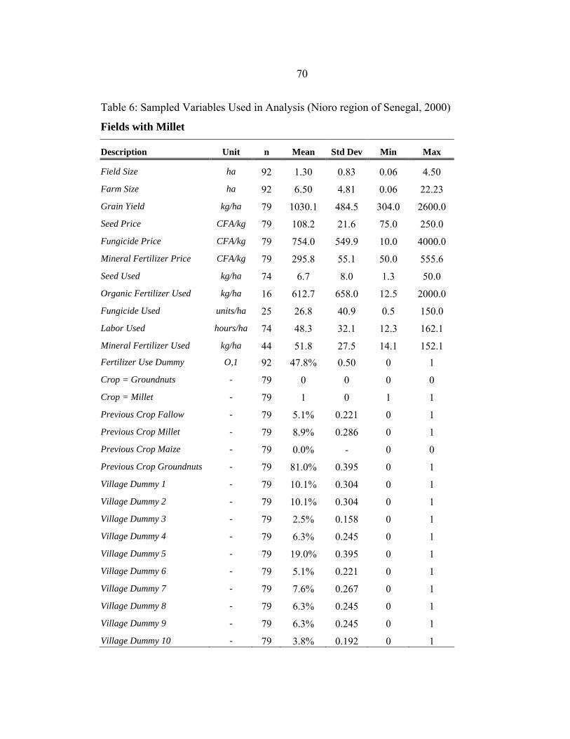
70
Table 6: Sampled Variables Used in Analysis (Nioro region of Senegal, 2000)
Fields with Millet
Description Unit n Mean Std Dev Min Max
Field Size ha 92 1.30 0.83 0.06 4.50 Farm Size ha 92 6.50 4.81 0.06 22.23 Grain Yield kg/ha 79 1030.1 484.5 304.0 2600.0 Seed Price CFA/kg 79 108.2 21.6 75.0 250.0 Fungicide Price CFA/kg 79 754.0 549.9 10.0 4000.0 Mineral Fertilizer Price CFA/kg 79 295.8 55.1 50.0 555.6 Seed Used kg/ha 74 6.7 8.0 1.3 50.0 Organic Fertilizer Used kg/ha 16 612.7 658.0 12.5 2000.0 Fungicide Used units/ha 25 26.8 40.9 0.5 150.0 Labor Used hours/ha 74 48.3 32.1 12.3 162.1 Mineral Fertilizer Used kg/ha 44 51.8 27.5 14.1 152.1 Fertilizer Use Dummy O,1 92 47.8% 0.50 0 1 Crop = Groundnuts - 79 0 0 0 0 Crop = Millet - 79 1 0 1 1 Previous Crop Fallow - 79 5.1% 0.221 0 1 Previous Crop Millet - 79 8.9% 0.286 0 1 Previous Crop Maize - 79 0.0% - 0 0 Previous Crop Groundnuts - 79 81.0% 0.395 0 1 Village Dummy 1 - 79 10.1% 0.304 0 1 Village Dummy 2 - 79 10.1% 0.304 0 1 Village Dummy 3 - 79 2.5% 0.158 0 1 Village Dummy 4 - 79 6.3% 0.245 0 1 Village Dummy 5 - 79 19.0% 0.395 0 1 Village Dummy 6 - 79 5.1% 0.221 0 1 Village Dummy 7 - 79 7.6% 0.267 0 1 Village Dummy 8 - 79 6.3% 0.245 0 1 Village Dummy 9 - 79 6.3% 0.245 0 1 Village Dummy 10 - 79 3.8% 0.192 0 1
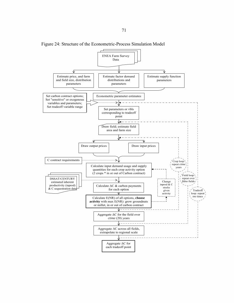
71
Figure 24: Structure of the Econometric-Process Simulation Model
Estimate factor demand distributions and
parameters
Estimate price, and farm and field size, distribution
parameters
Estimate supply function parameters
ENEA Farm Survey Data
Econometric parameter estimates
Calculate ∆C & carbon payments for each option
Set parameters or vbls corresponding to tradeoff
point
Draw field; estimate field area and farm size
Set carbon contract options; Set "sensitive" or exogenous
variables and parameters; Set tradeoff variable range
Draw output prices Draw input prices
Calculate input demand usage and supply quantities for each crop activity option (2 crops * in or out of Carbon contract)
Calculate E(NR) of all options, choose activity with max E(NR): grow groundnuts
or millet, in or out of carbon contract
Aggregate ∆C for the field over ctime (20) years
Aggregate ∆C across all fields, extrapolate to regional scale
Aggregate ∆C for each tradeoff point
C contract requirements
DSSAT/CENTURY estimated inherent
productivity (inprod) & C sequestration data
Change inprod & C
stocks given
activity
Crop loop: repeat ctime
years
Field loop: repeat over fldno fields
Tradeoff loop: repeat
tno times

72
Structure of the Analysis
Figure 24 shows the steps used to carry out this analysis. The simulation uses
estimated biophysical and economic parameters in order to simulate the land-use decisions
and corresponding outcomes for each field, across space and time. One hundred draws are
made from the sample set of fields. In order to simulate the spatial heterogeneity faced by
farmer, farm size, field area, and input prices are spatially varied.
Farm size and field size are modeled as spatially-varying lognormal distributions,
with the mean of the logged variable varying by village. These village effects were
estimated with OLS, and are reported in tables 7 and 8. Output and labor prices are
modeled as spatially varying log normal random variables. Village effects on seed,
fungicide, and fertilizer prices are estimated using OLS; these parameters are reported in
tables 9 to 11.
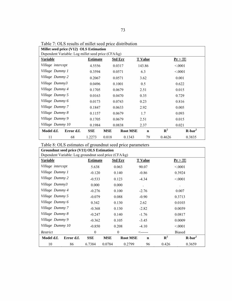
73
Table 7: OLS results of millet seed price distribution Millet seed price (V12) OLS Estimation Dependent Variable: Log millet seed price (CFA/kg) Variable Estimate Std Err T Value Pr > |T| Village intercept 4.5556 0.0317 143.86 <.0001 Village Dummy 1 0.3594 0.0571 6.3 <.0001 Village Dummy 2 0.2067 0.0571 3.62 0.001 Village Dummy3 0.0496 0.1001 0.5 0.622 Village Dummy 4 0.1705 0.0679 2.51 0.015 Village Dummy 5 0.0163 0.0470 0.35 0.729 Village Dummy 6 0.0173 0.0743 0.23 0.816 Village Dummy 7 0.1847 0.0633 2.92 0.005 Village Dummy 8 0.1157 0.0679 1.7 0.093 Village Dummy 9 0.1705 0.0679 2.51 0.015 Village Dummy 10 0.1984 0.0838 2.37 0.021 Model d.f. Error d.f. SSE MSE Root MSE n R2 R-bar2
11 68 1.2273 0.018 0.1343 79 0.4626 0.3835
Table 8: OLS estimates of groundnut seed price parameters Groundnut seed price (V11) OLS Estimation Dependent Variable: Log groundnut seed price (CFA/kg) Variable Estimate Std Err T Value Pr > |T| Village intercept 5.638 0.063 90.07 <.0001 Village Dummy 1 -0.120 0.140 -0.86 0.3924 Village Dummy 2 -0.533 0.123 -4.34 <.0001 Village Dummy3 0.000 0.000 . . Village Dummy 4 -0.276 0.100 -2.76 0.007 Village Dummy 5 -0.079 0.088 -0.90 0.3713 Village Dummy 6 0.342 0.130 2.62 0.0103 Village Dummy 7 -0.368 0.130 -2.82 0.0059 Village Dummy 8 -0.247 0.140 -1.76 0.0817 Village Dummy 9 -0.362 0.105 -3.45 0.0009 Village Dummy 10 -0.850 0.208 -4.10 <.0001 Restrict 0 0 <------ Biased Model d.f. Error d.f. SSE MSE Root MSE n R2 R-bar2
10 86 6.7384 0.0784 0.2799 96 0.426 0.3659

74
Table 9: OLS estimates of fungicide price parameters Groundnut fungicide price (V4) OLS Estimation Dependent Variable: fungicide units (CFA/unit) Variable Estimate Std Err T Value Pr > |T| Village intercept 5.363 0.349 15.380 <.0001 Village Dummy 1 0.942 0.780 1.210 0.230 Village Dummy 2 1.655 0.685 2.420 0.018 Village Dummy3 0.000 0.000 . . Village Dummy 4 -0.009 0.556 -0.020 0.987 Village Dummy 5 1.294 0.487 2.660 0.010 Village Dummy 6 1.083 0.726 1.490 0.140 Village Dummy 7 -1.600 0.726 -2.200 0.030 Village Dummy 8 1.178 1.157 1.020 0.312 Village Dummy 9 1.001 0.586 1.710 0.091 Village Dummy 10 0.852 1.157 0.740 0.464 Restriction 0 0 <------ Biased Model d.f. Error d.f. SSE MSE Root MSE n R2 R-bar2
10 83 201.9 2.4328 1.5597 93 0.2393 0.1568
Table 10: OLS estimation of mineral fertilizer price parameters Fertilizer NPK price (V6) OLS Estimation Dependent Variable: Log mineral fertilizer price (CFA/kg) Variable Estimate Std Err T Value Pr > |T| Village intercept 5.724 0.050 114.400 <.0001 Village Dummy 1 -0.010 0.099 -0.100 0.917 Village Dummy 2 0.055 0.094 0.590 0.556 Village Dummy3 0.004 0.224 0.020 0.988 Village Dummy 4 0.046 0.088 0.520 0.603 Village Dummy 5 -0.322 0.072 -4.490 <.0001 Village Dummy 6 -0.011 0.110 -0.100 0.918 Village Dummy 7 -0.070 0.102 -0.680 0.495 Village Dummy 8 -0.062 0.110 -0.570 0.571 Village Dummy 9 -0.469 0.092 -5.110 <.0001 Village Dummy 10 -0.027 0.147 -0.190 0.853 Model d.f. Error d.f. SSE MSE Root MSE n R2 R-bar2
11 164 15.5986 0.0951 0.3084 175 0.2544 0.209
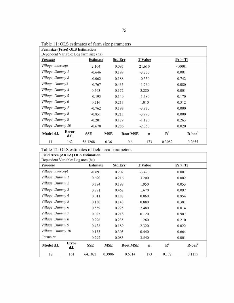
75
Table 11: OLS estimates of farm size parameters Farmsize (Fsize) OLS Estimation Dependent Variable: Log farm size (ha) Variable Estimate Std Err T Value Pr > |T| Village intercept 2.104 0.097 21.610 <.0001 Village Dummy 1 -0.646 0.199 -3.250 0.001 Village Dummy 2 -0.062 0.188 -0.330 0.742 Village Dummy3 -0.767 0.435 -1.760 0.080 Village Dummy 4 0.563 0.172 3.280 0.001 Village Dummy 5 -0.193 0.140 -1.380 0.170 Village Dummy 6 0.216 0.213 1.010 0.312 Village Dummy 7 -0.762 0.199 -3.830 0.000 Village Dummy 8 -0.851 0.213 -3.990 0.000 Village Dummy 9 -0.201 0.179 -1.120 0.263 Village Dummy 10 -0.670 0.286 -2.350 0.020
Model d.f. Error d.f. SSE MSE Root MSE n R2 R-bar2
11 162 58.3268 0.36 0.6 173 0.3082 0.2655
Table 12: OLS estimates of field area parameters Field Area (AREA) OLS Estimation Dependent Variable: Log area (ha) Variable Estimate Std Err T Value Pr > |T| Village intercept -0.691 0.202 -3.420 0.001 Village Dummy 1 0.690 0.216 3.200 0.002 Village Dummy 2 0.384 0.198 1.950 0.053 Village Dummy 3 0.771 0.462 1.670 0.097 Village Dummy 4 0.011 0.187 0.060 0.954 Village Dummy 5 0.130 0.148 0.880 0.381 Village Dummy 6 0.559 0.225 2.480 0.014 Village Dummy 7 0.025 0.218 0.120 0.907 Village Dummy 8 0.296 0.235 1.260 0.210 Village Dummy 9 0.438 0.189 2.320 0.022 Village Dummy 10 0.133 0.305 0.440 0.664 Farmsize 0.292 0.083 3.540 0.001
Model d.f. Error d.f. SSE MSE Root MSE n R2 R-bar2
12 161 64.1821 0.3986 0.6314 173 0.172 0.1155

76
For each field, farm size and field areas are drawn from the estimated distributions
which use village information. Fertilizer, seed and fungicide prices are estimated using the
OLS determined village effects. These parameters will remain with the field through all
years, through all tradeoff variable (carbon price) loops. For each growing season, output
and labour prices are sampled from non village-dependant distributions. Expected supply
and input use are simulated, given these sampled prices and estimated parameters of the
production models.
Expected net revenues (ENRs) for each crop are calculated using these calculated
production, input demand, and cost quantities. If alternative management options (such as
carbon sequestration contracts) are available to farmers, then the expected net returns will
be calculated for each available activity, for each crop, and the activity and crop
corresponding to the maximum ENR is selected.
After the model has simulated land usage, activity choice, production quantities,
input consumption and environmental changes for all draws from the sample, the same
procedure will be repeated on the same field for ctime cycles (20 years in this case). In
each subsequent year, output prices are again drawn, and the same economic parameters
are used to calculate ENRs for each activity. The activity choice simulated in the previous
year affects successive ENRs, through crop rotational effects (estimated econometrically in
the economic models), and changes in inherent productivity. If an activity that altered the
inherent productivity path, such as entering a carbon contract, was chosen previously, then
this will impact expected productivity in the next year.

77
In this simulation, carbon prices are varied from zero to $200/tonne (0 to 100,000
CFA/tonne) to derive carbon supply curves. In the simulation model structure, the carbon
price is defined as a “tradeoff variable” and each tradeoff point corresponds to a different
price. For each tradeoff point, another loop of the model (i fields * ctime years) is run, and
the results are aggregated. Results are scaled up to the regional level (there are
approximately 103,000 hectares of millet and groundnut production in the Nioro region),
and in this way carbon supply curves are generated.
Biophysical Parameters: Inherent Productivity_________________
Inherent productivity (INPROD) values were estimated using the
DSSAT/CENTURY model, as described in Chapter 1, using soils and climate data for each
village. These values, which are the predicted yields for each crop, exhibit relatively little
variation. There are five different soil types, and therefore five different simulated inherent
productivity and carbon paths for each management practice. Figure 25 shows the five
initial inherent productivities for both of the crops. This grouping of the inherent
productivities leads to clusters of farms with identical proxies for biophysical parameters.
When farmers make discrete choices (such as whether to use fertilizer, or participate in a
carbon contract, etc.), the inherent productivity variable can cause simulated groups of
farmers to make similar decisions. Later in this analysis, this causes supply curves to
assume a step-function shape (for example, see Figure 27).

78
Figure 25: Inherent productivity data, by soil type and crop
0
200
400
600
800
1000
1200
1400
0 2 4 6 8Soil types
Initi
al IN
PRO
Ds
Millet Initial INPROD Peanut Initial INPROD
size of bubble = f(number of fields in group)
Econometric Specification and Estimation of Groundnut and Millet Production Models__
A key issue identified in Chapter 2 is the low, and often zero, rates of mineral
fertilizer use in the Senegal groundnut/millet system. Conventional, neoclassical
production models do not allow for zero input use. This section describes how a
conventional log-linear specification of factor demand and output supply equations was
adapted to account for the zero-input problem.
The approach taken here is a pragmatic one, aimed at the development of a well-
behaved simulation model that captures farmers’ behavior in this system. Elaborate
econometric procedures, e.g. with mixed discrete-choice and continuous choice equations,
are not considered for two practical reasons. First, the data available for this analysis

79
undoubtedly contain significant measurement errors; and second, the simulation of
complex systems discrete and continuous choice models is not empirically tractable.
OLS (Ordinary Least Squares) was used to estimate each of the economic
equations, including input demand functions and supply functions. These are modeled as
constant elasticity functions with non additive error terms. Given these non additive errors,
these functions are non linear in the parameters, and therefore nonlinear least squares is
used. These errors are assumed to have mean (0) and constant variance. Equations were
estimated separately, and most equations contained non-linear elements. Generally, input
demand is a function of input prices, output prices, and agronomic potential and other fixed
effects.
Table 13 shows the OLS results of demand for seed and labor in the groundnut and
millet crops.

80
Table 13: OLS estimates of groundnut seed demand parameters Groundnut seed demand (X1) Non-Linear OLS Estimation Dependent Variable: groundnut seed (kg/ha) Variable Estimate Std Err T Value Pr > |T| Intercept -4.968 5.701 -0.870 0.387 Log (area) -0.302 0.064 -4.740 <.0001 Log (seed price) -1.046 0.159 -6.570 <.0001 Log (fertilizer price) 0.197 0.140 1.410 0.163 Fungicide use dummy -0.141 0.094 -1.500 0.137 Previous millet dummy -0.127 0.137 -0.930 0.358 Log (farm size) 0.135 0.063 2.160 0.034 Log (inherent prod.) 2.043 0.848 2.410 0.019 Model d.f. Error d.f. SSE MSE Root MSE n R2 R-bar2
8 69 85767.3 1243 35.2563 77 0.4822 0.4297
Table 14: OLS estimates of labor demand parameters in groundnut fields Groundnut labor demand (X5) Non-Linear OLS Estimation Dependent Variable: groundnut labour (person days/ha) Variable Estimate Std Err T Value Pr > |T| Intercept 13.208 5.617 2.350 0.022 Log (area) -0.348 0.069 -5.070 <.0001 Log (seed price) -0.439 0.155 -2.840 0.006 Fungicide use dummy -0.045 0.080 -0.560 0.576 Log (fertilizer price) -0.507 0.129 -3.920 0.000 Previous millet dummy -0.028 0.146 -0.190 0.849 Log (farm size) -0.266 0.072 -3.680 0.001 Log (inherent prod.) -0.472 0.878 -0.540 0.593 Model d.f. Error d.f. SSE MSE Root MSE n R2 R-bar2
8 61 34134 559.6 23.6553 69 0.662 0.6232
Table 15: OLS estimates of millet seed demand parameters Millet seed demand (X1) Non-Linear OLS Estimation Dependent Variable: millet seed (kg/ha) Variable Estimate Std Err T Value Pr > |T| Intercept -4.304 14.308 -0.300 0.764 Log (area) -0.278 0.191 -1.460 0.149 Previous groundnut dummy -0.007 0.263 -0.030 0.980 Log (farm size) -0.198 0.112 -1.770 0.081 Log (inherent prod.) 0.981 2.171 0.450 0.653 Model d.f. Error d.f. SSE MSE Root MSE n R2 R-bar2
5 83 3690.5 44.4636 6.6681 88 0.2096 0.1715
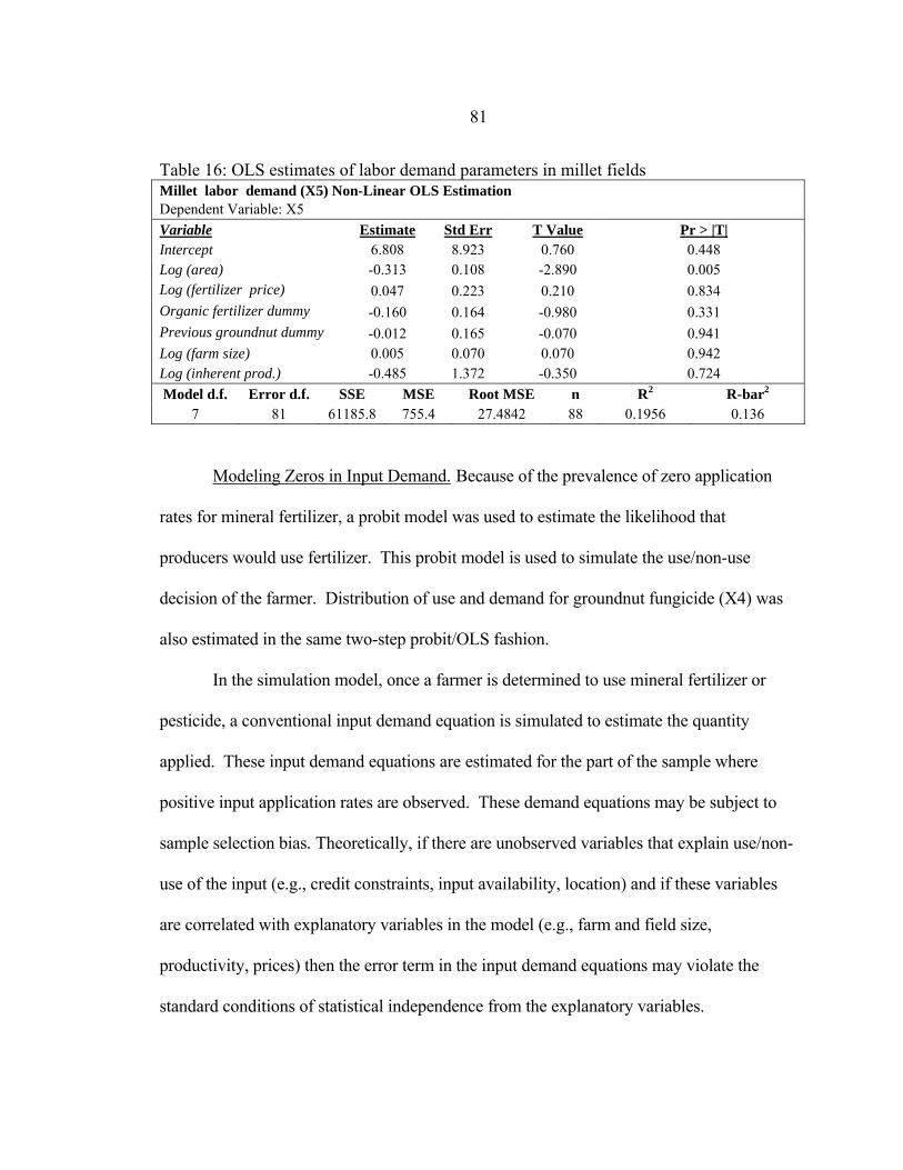
81
Table 16: OLS estimates of labor demand parameters in millet fields Millet labor demand (X5) Non-Linear OLS Estimation Dependent Variable: X5 Variable Estimate Std Err T Value Pr > |T| Intercept 6.808 8.923 0.760 0.448 Log (area) -0.313 0.108 -2.890 0.005 Log (fertilizer price) 0.047 0.223 0.210 0.834 Organic fertilizer dummy -0.160 0.164 -0.980 0.331 Previous groundnut dummy -0.012 0.165 -0.070 0.941 Log (farm size) 0.005 0.070 0.070 0.942 Log (inherent prod.) -0.485 1.372 -0.350 0.724 Model d.f. Error d.f. SSE MSE Root MSE n R2 R-bar2
7 81 61185.8 755.4 27.4842 88 0.1956 0.136
Modeling Zeros in Input Demand. Because of the prevalence of zero application
rates for mineral fertilizer, a probit model was used to estimate the likelihood that
producers would use fertilizer. This probit model is used to simulate the use/non-use
decision of the farmer. Distribution of use and demand for groundnut fungicide (X4) was
also estimated in the same two-step probit/OLS fashion.
In the simulation model, once a farmer is determined to use mineral fertilizer or
pesticide, a conventional input demand equation is simulated to estimate the quantity
applied. These input demand equations are estimated for the part of the sample where
positive input application rates are observed. These demand equations may be subject to
sample selection bias. Theoretically, if there are unobserved variables that explain use/non-
use of the input (e.g., credit constraints, input availability, location) and if these variables
are correlated with explanatory variables in the model (e.g., farm and field size,
productivity, prices) then the error term in the input demand equations may violate the
standard conditions of statistical independence from the explanatory variables.

82
One procedure used for sample selection correction is the Heckit method, after the
work of Heckman (Wooldridge, 2003). The Heckit procedure was run on the model, by
first estimating probit equations, calculating the inverse Mill's ratio, and then estimating the
input demand equations including the inverse Mill's ratio as an explanatory variable. The
estimated parameters of the inverse Mill's ratio were statistically insignificant, indicating
that error covariance was not a problem in the model. In addition to this, the other
parameter estimates had similar values to those in the truncated OLS model. As a result, a
probit and OLS method was used to estimate these discrete choice demand models. Table
17 and Table 18 show the estimated probit models of fertilizer usage.
Table 17: Probit Model for fertilizer use in groundnut fields (modeling the probability of no fertilizer usage: X6D1=0)
Variable
DF
Estimate
Std Error
95% Confidence Limits
Chi Square
Pr > ChiSq
- 1 -4.728 5.795 -16.086 6.630 0.670 0.415
Log(field area) 1 -0.414 0.221 -0.847 0.020 3.500 0.061
Log(farm area) 1 0.271 0.251 -0.220 0.762 1.170 0.280
Log(fertilizer price) 1 1.608 0.528 0.574 2.642 9.290 0.002
Log(inherent productivity)
1 -0.670 0.762 -2.163 0.824 0.770 0.380
Dependent Variable: X6D1 Name of Distribution: Normal
n total, n with X6>0: 79, 49 Log Likelihood: - 45.8127

83
Table 18: Probit Model for fertilizer use in millet fields (modeling the probability of no fertilizer usage: X6D2=0)
These probit models of fertilizer usage provide economically sensible parameter
estimates. In the case of groundnuts, only field area and fertilizer price parameters were
statistically significant. Field area is positively correlated with usage, which runs against
the conventional wisdom that small plots, generally closer to the home, tend to be farmed
more intensely. Higher fertilizer prices, of course, are associated with non-usage. This is
consistent with the ideas put forth in Chapter 2, namely that farmers who face high prices
are more likely to be at a corner solution. Although the inherent productivity parameter
estimate is not statistically significant, it is negative, which is consistent with the idea that
fertilizer use is positively related to productivity potential. Labor costs and time constraints
would create thresholds, where it could be more productive for a farmer to apply more or
all of their fertilizer on some fields, and none at all on others, rather than a lower average
level across all fields.
Variable
DF
Estimate
Std Error
95% Confidence Limits
Chi Square
Pr > ChiSq
- 1 34.951 19.628 -3.519 73.421 3.170 0.075 Log(field area) 1 -0.110 0.227 -0.555 0.335 0.240 0.628 Log(farm area) 1 0.021 0.178 -0.327 0.369 0.010 0.906 Log(seed price) 1 -2.770 1.085 -4.895 -0.644 6.520 0.011 Log(fertilizer price) 1 0.999 0.569 -0.116 2.113 3.080 0.079 Log(inherent productivity) 1 -4.205 2.779 -9.653 1.242 2.290 0.130
Dependent Variable: X6D2 Name of Distribution: Normal
n total, n with X6>0: 92, 44 Log Likelihood: -57.437
84
Table 18 shows the results of the millet probit model where the intercept, seed
price, fertilizer price and inherent productivity parameter estimates were statistically
significant. As seed prices increase, the probability of fertilizer usage increases (as non-
usage drops). This could be the result of farmers expecting higher output prices, since
millet seed and millet output markets are positively related. The fertilizer price and
inherent productivity parameters have the same signs, and likely the same causes, as in the
groundnut case.
The Fertilizer Demand Function. The following mineral fertilizer demand function
was estimated using OLS, with the sample truncated to where fertilizer usage (X6) is
greater than 0.
Generally, Mineral Fertilizer Quantity = f {intercept, log (field area), log (groundnut
seed price), log (fertilizer price), previous millet crop dummy variable, log
(farm size), log (inherent productivity in year 1)}
From the factor share equation:
( F01 + FAREA1*ln(AREA) + FV11*ln(V1) + FV61*ln(V6) + FPRML1*PR_ML + FFSIZE1*ln(FSIZE) + FINP1*ln(INP101))6X e=
Table 19 shows the estimated results of the fertilizer demand equations. In the
groundnut model, the estimated parameters for field area, fertilizer price, and the previous
crop being millet dummy were statistically significant. In the case of millet, the parameters
for field area, seed price, and farm area were significant.
In Senegal, larger fields are typically located further away from the village, and
tend to be farmed less intensively than those closer by. This is consistent with the
estimated parameters, FAREA1 and FAREA2, which were (-.39) and (-.57) respectively.
85
The farm size parameter was significant and positive in the millet equation. In this case,
farm size could be a proxy for greater farm household wealth, which would lead to more
access to credit and capital to make fertilizer purchases. In the case of groundnuts, the
parameter for fertilizer price was highly significant and negative. This demonstrates
downward-sloping input demand curves. For millet, seed price was negative and
significant. This is likely because farmers substitute seed density for fertilizer usage (Kelly
et al., 1996). In groundnuts, the seed price parameter was small, positive and insignificant.
Finally, in the groundnut equation, the millet rotation dummy variable was negative and
significant. Two factors influence this effect; the agronomics of crop rotations, and
financial constraints. If farmers grew millet the year before, it is likely that their soils have
lower nitrogen balances than if they grew groundnuts (groundnuts are a leguminous crop,
which has nitrogen fixing capability). For this reason, we could expect a positive value on
this parameter. However, because groundnuts are a cash crop, and millet is not, it is likely
that farmers will have lower financial reserves after growing millet. This second effect
appears to be dominant, and for this reason we see a negative algebraic sign on this
parameter. The statistical insignificance of inherent productivity is of concern. This was
probably a result of little variation in inherent productivity numbers across fields

86
Table 19: OLS estimates of groundnut fertilizer demand parameters (where X6>0) SAS Non Linear OLS Model Procedure – Groundnut Model
Dependent Variable: fertilizer use (kg/ha) where X6>0 (n=49/79 groundnut fields)
Variable Estimate Std Err T Value Pr > |T|
Intercept 7.22603 4.9777 1.45 0.154
Log(field area) -0.3914 0.1487 -2.63 0.0118
Log(groundnut seed price) 0.098841 0.4337 0.23 0.8208
Log(fertilizer price) -0.81154 0.2842 -2.86 0.0067
Previous millet crop dummy -0.57985 0.264 -2.2 0.0336
Log(farm area) -0.19658 0.1658 -1.19 0.2424
Log(inherent productivity) 0.203069 0.5685 0.36 0.7227
Model d.f. Error d.f. SSE MSE Root MSE n R2 R-bar2
7 42 49815 1186.1 34.4394 49 0.611 0.5554
Table 20: OLS estimates of millet fertilizer demand parameters (where X6>0) SAS Non Linear OLS Model Procedure – Millet Model
Dependent Variable: fertilizer use (kg/ha) where X6>0 (n=44/93 millet fields)
Variable Estimate Std Err T Value Pr > |T|
Intercept 10.19454 8.6724 1.18 0.2473 Log(field area) -0.56996 0.1338 -4.26 0.0001 Log(millet seed price) -1.05445 0.526 -2.000 0.052 Log(fertilizer price) -0.1323 0.106 -1.250 0.218 Log(organic fertilizer) -0.07754 0.162 -0.480 0.635 Log(farm area) 0.166472 0.092 1.820 0.077 Log(inherent productivity) -0.12485 1.214 -0.100 0.919
Model d.f. Error d.f. SSE MSE Root MSE n R2 R-bar2
7 37 18130.5 490 22.136 44 0.442 0.351

87
Table 21: Estimated groundnut fungicide use discrete choice and input demand parameters
Probit Model for Fungicide Usage with the Groundnut Crop (modeling the probability of no fungicide usage: X4D=0)
Variable
DF
Estimate
Std Error
95% Confidence Limits
Chi Square
Pr > ChiSq
- 1 36.73 20.23 -2.92 76.39 3.30 0.07
Log(farm area)
1 -0.24 0.23 -0.68 0.21 1.08 0.30
Log(fertilizer price)
1 -1.38 0.46 -2.27 -0.49 9.18 0.00
Log(inherent productivity) 1 -4.17 2.98 -10.01 1.67 1.96 0.16
Dependent Variable: X4D Name of Distribution:
Normal
n total, n with X4>0: 79,34 Log Likelihood: -46.7170
Groundnut Model : SAS Non Linear OLS Model Procedure
Dependant Variable: fungicide units/ha, where X4>0 (34/79 fields)
Variable Estimate Std Err T Value Pr > |T|
Intercept 8.890 12.207 0.730 0.473
Log(field area) -0.117 0.126 -0.930 0.361
Log(fertilizer price) -1.033 0.422 -2.450 0.021
Previous millet dummy -0.166 0.181 -0.920 0.367
Log (farm size) 0.236 0.151 1.560 0.131
Log (inherent prod.) 0.148 1.938 0.080 0.940 Model
d.f. Error d.f. SSE MSE Root MSE n R2 R-bar2
6 28 33057.6 1180.6 34.3603 34 0.2648 0.1335

88
Supply Equations
Conventional production function or supply function models do not allow for zero
input use. To estimate fertilizer productivity with both zero and positive application rates,
the supply function is specified as a function of a (0,1) dummy variable for fertilizer use.
The parameter on this dummy variable measures the average productivity of fertilizer in the
fertilizer-using group. To simulate fertilizer supply response, this mean productivity of
fertilizer is applied to all observations that use more than the mean application rate (X6*) in
the fertilizer-using group. For application rates below X6*, fertilizer productivity is
approximated by a linear relationship between zero and the mean level for the user group
(see Figure 26).
Figure 26: Crop yield and carbon sequestration returns to fertilizer use
Cro
p Y
ield
s So
il C
sequ
este
red
per h
a
Fertilizer usage kg/ha
X6
C (t/ha), CropYield
(kg/ha)
0 69
Functional form used in simulation
Possible theoretical functions with
diminishing returns

89
Table 22 shows the parameter estimates of the supply function. The parameter
QX6D1 is estimated to be 0.23, implying that farmers that use mineral fertilizer in
groundnut production obtain on average approximately 23 percent higher yield than
farmers not using fertilizer.
Table 22: OLS estimated groundnut grain supply parameters
Groundnut Grain Supply (QR1) Non-Linear OLS Estimation Dependent Variable: groundnut grain yield (kg/ha) Variable Estimate Std Err T Value Pr > |T|
Intercept 3.275 0.607 5.400 <.0001 Log(field area) -0.096 0.045 -2.130 0.036 Log(groundnut seed price) 0.015 0.103 0.150 0.883 Fertilizer use dummy 0.228 0.069 3.310 0.001 Previous millet dummy 0.181 0.089 2.040 0.045 Log(Inherent productivity) 0.500 0.000 . . Restriction 3.081 1.732 1.780 0.075 Model
d.f. Error d.f. SSE MSE Root MSE n R2 R-bar2
5 74 7179536 97021 311.5 79 0.1786 0.1342
Table 23: OLS estimated groundnut residue supply parameters Groundnut Residue Hay Supply (QB1) Non-Linear OLS Estimation Dependent Variable: groundnut residue yield (kg/ha) Variable Estimate Std Err T Value Pr > |T|
Intercept 0.192 0.942 0.200 0.839 Log(field area) -0.071 0.053 -1.350 0.182 Log(groundnut grain supply) 0.515 0.135 3.810 0.000 Fertilizer use dummy 0.239 0.087 2.750 0.007
Log(Inherent productivity) 0.500 0.000 . . Restriction 3.296 1.515 2.180 0.029 Model d.f. Error d.f. SSE MSE Root MSE n R2 R-bar2
4 75 1.9E+07 257061 507 79 0.2972 0.2691
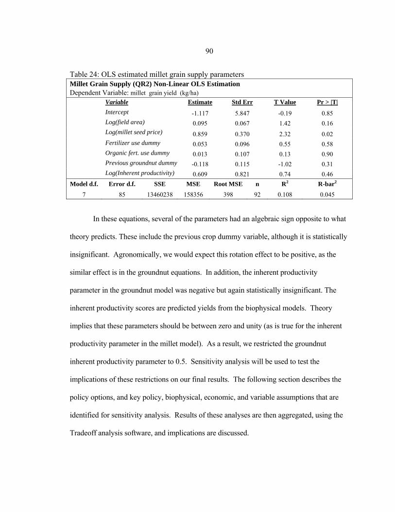
90
Table 24: OLS estimated millet grain supply parameters Millet Grain Supply (QR2) Non-Linear OLS Estimation Dependent Variable: millet grain yield (kg/ha) Variable Estimate Std Err T Value Pr > |T|
Intercept -1.117 5.847 -0.19 0.85 Log(field area) 0.095 0.067 1.42 0.16
Log(millet seed price) 0.859 0.370 2.32 0.02 Fertilizer use dummy 0.053 0.096 0.55 0.58 Organic fert. use dummy 0.013 0.107 0.13 0.90 Previous groundnut dummy -0.118 0.115 -1.02 0.31 Log(Inherent productivity) 0.609 0.821 0.74 0.46 Model d.f. Error d.f. SSE MSE Root MSE n R2 R-bar2
7 85 13460238 158356 398 92 0.108 0.045
In these equations, several of the parameters had an algebraic sign opposite to what
theory predicts. These include the previous crop dummy variable, although it is statistically
insignificant. Agronomically, we would expect this rotation effect to be positive, as the
similar effect is in the groundnut equations. In addition, the inherent productivity
parameter in the groundnut model was negative but again statistically insignificant. The
inherent productivity scores are predicted yields from the biophysical models. Theory
implies that these parameters should be between zero and unity (as is true for the inherent
productivity parameter in the millet model). As a result, we restricted the groundnut
inherent productivity parameter to 0.5. Sensitivity analysis will be used to test the
implications of these restrictions on our final results. The following section describes the
policy options, and key policy, biophysical, economic, and variable assumptions that are
identified for sensitivity analysis. Results of these analyses are then aggregated, using the
Tradeoff analysis software, and implications are discussed.
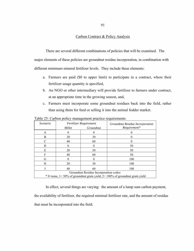
91
Carbon Contract & Policy Analysis
There are several different combinations of policies that will be examined. The
major elements of these policies are groundnut residue incorporation, in combination with
different minimum mineral fertilizer levels. They include these elements:
a. Farmers are paid ($0 to upper limit) to participate in a contract, where their
fertilizer usage quantity is specified,
b. An NGO or other intermediary will provide fertilizer to farmers under contract,
at an appropriate time in the growing season, and,
c. Farmers must incorporate some groundnut residues back into the field, rather
than using them for feed or selling it into the animal fodder market.
Table 25: Carbon policy management practice requirements Scenario Fertilizer Requirement
Millet Groundnut Groundnut Residue Incorporation
Requirement* A 0 0 0 B 20 30 0 C 40 60 0 D 0 0 50 E 20 30 50 F 40 60 50 G 0 0 100 H 20 30 100 I 40 60 100
Groundnut Residue Incorporation codes: * 0=none, 1= 50% of groundnut grain yield, 2= 100% of groundnut grain yield
In effect, several things are varying: the amount of a lump sum carbon payment,
the availability of fertilizer, the required minimal fertilizer rate, and the amount of residue
that must be incorporated into the field.
92
Implementation Issues
Buyers of carbon contracts would not want farmers to opt in and out of carbon
sequestration programs to ensure that the carbon is stored permanently.
Initial information problems are not significant in the area of study because almost
no farmers are in the "incumbent" position of already sequestering carbon. Residue
incorporation is rare in the groundnut basin, and this is the catalyst which leads most of the
carbon sequestration in this agricultural system. Even farmers using 70 kg/ha of fertilizer
can greatly increase their net carbon sequestration rate by incorporating residue. As a
result, there are no perverse incentives for incumbent fertilizer users to temporarily stop or
misrepresent their fertilizer usage in order to qualify for carbon contracts.
Contract Design and Incentives
An important set of contract design issues concerns the flexibility farmers have to
enter and exit contracts, whether farmers will be penalized for defaulting on contracts, and
the impact that flexibility has for the amount of carbon that is sequestered. We assume that
contracts would require farmers to maintain the prescribed practices (fertilizer applications
and residue incorporation) for the duration of the contract. Carbon accumulation is a
relatively slow process, often taking 20 to 30 years for soil carbon to converge to a new
equilibrium after farmers change practices.
Moreover, as explained in Chapter 1, soil carbon is likely to be lost if those
practices are not continuously maintained. Therefore, we would expect carbon contracts to
require maintaining practices for a relatively long period, and contract duration is assumed

93
to be 20 years in this analysis. However, farmers may either choose not to maintain the
practice continuously, or may not be able to do so, because of unanticipated changes in
economic or environmental conditions. When this happens, one could argue in principle
that farmers should be penalized for the carbon that is released back into the atmosphere. It
is not clear, however, whether it would be politically or administratively feasible to
implement such penalties. In this analysis we consider two possible approaches to contract
default. First, farmers are required to stay in the contract for the duration of the contract;
opting out is not an option (this will be used in most of the analysis). Second, farmers may
be allowed to enter and leave contracts without penalty, but when they stop complying with
the practices specified by the contract, they will not receive payments.
Carbon Rates and Carbon Payments. To calculate the carbon payment, changes in
carbon sequestration rates had to be estimated. The DSSAT/CENTURY crop and soil
carbon model estimated trends in soil carbon that were negative for all dataset and policy
management practices, with the exception of policy I.
Figure 6 (p. 24) shows that Carbon changes are approximately a linear function of
fertilizer usage and residue incorporation, in the form:
carbon=α+β*X6,
given a residue incorporation level (α and β vary with each level of residue incorporation).
The carbon rate attributed to using 30 kg/ha fertilizer is approximately the average
of the 0 and 60 kg/ha rates, given the same residue incorporation level. The annual
expected change in carbon for policy is modeled to be:

94
bcratep= (estimated carbon year 20- estimated carbon year 1)/20,
where p denotes the management practice prescribed by the contract
Ecratep is the annual expected change in carbon, relative to status quo (practice A):
ecratep= bcratep- bcrateA.
Annual carbon changes are calculated by taking the intercept (points A, D, and G on Figure
6), where fertilizer=0 for each residue level, and calculating a slope term for the function
by averaging the ecrates of the 0 and 60 kg/ha practices. For example, if all groundnut
residues are incorporated, (res_inc = 2), then the annual carbon change is:
_ 2
( - )( 6) 6
60 /i g
res inc g
ecrate ecrateCarbon X ecrate X
kg ha= = + ∗ .
To calculate the change in Carbon, relative to what it would have been outside of the
policy, we calculate the amount of carbon that would have been sequestered otherwise
(with no residue incorporation), and subtract that from the calculation above.
_ 2 _ 0 ( 6) ( 6 ) ( 6)res inc res incDCarb X Carbon X N Carbon X= == − ,
where X6N is the fertilizer used in contract, and X6 is the amount of fertilizer that would
have been used otherwise.
Finally, carbon payments were calculated by multiplying the price of carbon by the
calculated Dcarb.
95
Results of Simulation
The simulation was run across 21 tradeoff points, where the price of carbon per
tonne ranged from $0 to $200 USD; over 100 sample field draws; over 20 years. 31
scenarios, with different sets of policy restrictions, prices and other parameters of interest,
were run for the sensitivity analysis of the simulation results. SAS (v.9) was used to
estimate parameters, and run the simulations.
Base Policy Results
To begin, the nine carbon contract policy scenarios discussed earlier in this chapter
were simulated. Figure 27 and Figure 28 show the carbon supply curves simulated for the
Nioro region. With Policy A, which required no residue incorporation and had no fertilizer
requirements or provision, 0% of farmers participated and zero carbon was supplied. This
is to be expected, as it models the status quo, and without further incentives, farmers have
no reason to change practices. Policies B and C supplied trivial amounts of carbon, both
due to the very low carbon sequestration potential of those management practices. The
simulated supply curves are upward sloping, and diverge because of the differing carbon
potential of each policy. For example, contract I (fertilizer = 60, 40; res_inc=2) will
generate more per hectare than policies, such as E and H, which use half as much residue.
All policies with positive residue incorporation exhibited upward sloping supply
curves that supplied positive amounts of carbon at all positive price, even $0/t. As
described earlier, the bunching of the inherent productivity observations leads to clusters of
farms with identical proxies for biophysical parameters. Because of this, when farmers

96
make discrete choices, such as whether to participate in a carbon contract, the inherent
productivity variable can cause simulated groups of farmers to make similar decisions.
This causes the step-function shape that can be observed in the estimated supply curves.
Figure 27: Carbon supply with 6 residue-incorporating carbon contract policies
$-
$20
$40
$60
$80
$100
$120
$140
$160
$180
$200
- 200,000 400,000 600,000 800,000 1,000,000 1,200,000 1,400,000
Carbon (t)
$US/
t
D E F G H I
Policy: (groundnut fert kg/ha, millet fert kg/ha; R=residue incorporation) D: 0, 0; R=50% G: 0, 0; R=100%
E: 30, 20; R=50% H: 30,20; R=100% F: 60, 40; R=50% I: 60, 40; R=100%

97
Figure 28: Detail of carbon supply with 6 residue-incorporating carbon contract policies
$-
$5
$10
$15
$20
$25
$30
$35
$40
$45
$50
- 100,000 200,000 300,000 400,000 500,000 600,000
Carbon (t)
$US/
t
D E F G H I
Policy: (groundnut fert kg/ha, millet fert kg/ha; R=residue incorporation) D: 0, 0; R=50% G: 0, 0; R=100%
E: 30, 20; R=50% H: 30,20; R=100% F: 60, 40; R=50% I: 60, 40; R=100%
Figure 29: Contract participation in 6 residue incorporating carbon contract policies
$-
$20
$40
$60
$80
$100
$120
$140
$160
$180
$200
0% 10% 20% 30% 40% 50% 60% 70% 80% 90% 100%
% Participation
$US/
t
D E F G H I
Policy: (groundnut fert kg/ha, millet fert kg/ha; R=residue incorporation) D: 0, 0; R=50% G: 0, 0; R=100%
E: 30, 20; R=50% H: 30,20; R=100% F: 60, 40; R=50% I: 60, 40; R=100%

98
Figure 27, Figure 28, and Figure 29 show that contract participation with policies D
to I is positive when the price of carbon is $0/t. Farmers enter contracts for access to
fertilizer, even when carbon payments are zero, which implies that constraints on access to
fertilizer are relaxed with participation in carbon contracts, as hypothesized in Chapter 2.
Once these policies relaxed supply constraints, farmers increased their usage.
Contracts D and G, which require 0 fertilizer and residue incorporation levels 1 and
2, respectively, encourage more participation and C sequestration than their higher fertilizer
counterparts at the $0/t carbon price level. In the case of D and G, because farmers are not
forced to incorporate higher levels of fertilizer, but still have access to whatever fertilizer
they require; more farmers will enter these contracts at low carbon price levels. With all
contracts, participation and carbon supply increase with the price of carbon. Figure 27
shows that at higher price levels, more input use (i.e. policy I) results in more carbon
sequestration (i.e. policy E).
Sensitivity Analysis
Not all variables and parameters used in the analysis had known distributions, either
because they could not be statistically estimated, or perhaps because the statistically
estimated values were suspect. Sensitivity analysis is used to asses the affects of these
parameters. From this, we can compare and see how robust the original results of the
previous section are to our assumptions. Table 26 contains a complete listing of scenarios
tested.

99
Table 26: Scenario guide
Scenario X6C RES_INC TRANCOST MAN_CST PB1C X6KINK1 X6KINK2 QINP1 QBINP1 Exit & Entry Groundnuts Millet
A 0 0 0 1000 110 1 69 48 0.5 0.5 restricted B 30 20 0 1000 110 1 69 48 0.5 0.5 restricted C 60 40 0 1000 110 1 69 48 0.5 0.5 restricted D 0 0 1 1000 110 1 69 48 0.5 0.5 restricted E 30 20 1 1000 110 1 69 48 0.5 0.5 restricted F 60 40 1 1000 110 1 69 48 0.5 0.5 restricted G 0 0 2 1000 110 1 69 48 0.5 0.5 restricted H 30 20 2 1000 110 1 69 48 0.5 0.5 restricted I 60 40 2 1000 110 1 69 48 0.5 0.5 restricted
FT1 60 40 1 5000 110 1 69 48 0.5 0.5 restricted IT1 60 40 2 5000 110 1 69 48 0.5 0.5 restricted
FL90 60 40 1 1000 90 1 69 48 0.5 0.5 restricted IL90 60 40 2 1000 90 1 69 48 0.5 0.5 restricted
FL150 60 40 1 1000 150 1 69 48 0.5 0.5 restricted IL150 60 40 2 1000 150 1 69 48 0.5 0.5 restricted IPB50 60 40 2 1000 110 .5 69 48 0.5 0.5 restricted IPB90 60 40 2 1000 110 .9 69 48 0.5 0.5 restricted IPB110 60 40 2 1000 110 1.1 69 48 0.5 0.5 restricted IPB150 60 40 2 1000 110 1.5 69 48 0.5 0.5 restricted IPB200 60 40 2 1000 110 2 69 48 0.5 0.5 restricted IPB250 60 40 2 1000 110 2.5 69 48 0.5 0.5 restricted IKINK9 60 40 2 1000 110 1 62 43 0.5 0.5 restricted
IKINK12 60 40 2 1000 110 1 83 58 0.5 0.5 restricted FPARM25 60 40 1 1000 110 1 69 48 0.25 0.25 restricted IPARM25 60 40 2 1000 110 1 69 48 0.25 0.25 restricted FPARM75 60 40 1 1000 110 1 69 48 0.75 0.75 restricted IPARM75 60 40 2 1000 110 1 69 48 0.75 0.75 restricted INOUT_F 60 40 1 1000 110 1 69 48 0.5 0.5 free INOUT_I 60 40 2 1000 110 1 69 48 0.5 0.5 free

100
Variables of Interest for Sensitivity Analysis
• X6C. This is the minimum amount of fertilizer that must be applied if
participating in the carbon contract. Farmers participating in contracts will
have access to any amount of fertilizer equal or greater than X6C. This will
be available to farmers at prevailing (sampled from the dataset) prices.
• RES_INC. This indicates how much groundnut residue farmers must
incorporate into the soil. 0, 1, 2 indicate 0%, 50% and 100% of yield
respectively.
• TRANCOST. This is the cost of participating in carbon contracts. We
assume that when carbon prices are greater than zero, there will be a lump-
sum transaction cost applied each year.
• MAN_CST. This parameter is used to scale labor cost in order and test the
results’ sensitivity to this input.
• PB1C. This parameter is a scaling factor on the market price of crop
residues.
• X6KINK1, X6KINK2. These are the points at which the fertilizer
response functions concatenate, as discussed before and shown in Figure 26.
• QINP1. This inherent productivity parameter in the groundnut supply
function was estimated to be negative , but not statistically significant.
Agronomically, this is not possible, so three values between 0 and 1 will be
tested.
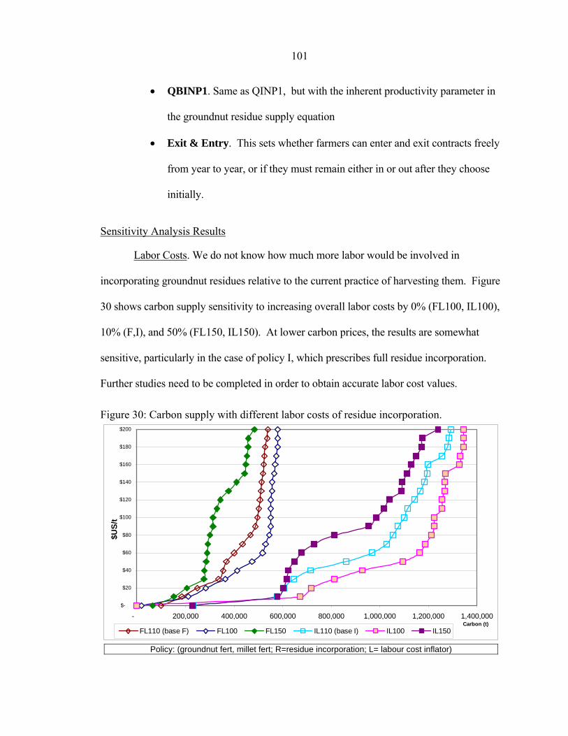
101
• QBINP1. Same as QINP1, but with the inherent productivity parameter in
the groundnut residue supply equation
• Exit & Entry. This sets whether farmers can enter and exit contracts freely
from year to year, or if they must remain either in or out after they choose
initially.
Sensitivity Analysis Results
Labor Costs. We do not know how much more labor would be involved in
incorporating groundnut residues relative to the current practice of harvesting them. Figure
30 shows carbon supply sensitivity to increasing overall labor costs by 0% (FL100, IL100),
10% (F,I), and 50% (FL150, IL150). At lower carbon prices, the results are somewhat
sensitive, particularly in the case of policy I, which prescribes full residue incorporation.
Further studies need to be completed in order to obtain accurate labor cost values.
Figure 30: Carbon supply with different labor costs of residue incorporation.
$-
$20
$40
$60
$80
$100
$120
$140
$160
$180
$200
- 200,000 400,000 600,000 800,000 1,000,000 1,200,000 1,400,000Carbon (t)
$US/
t
FL110 (base F) FL100 FL150 IL110 (base I) IL100 IL150
Policy: (groundnut fert, millet fert; R=residue incorporation; L= labour cost inflator)
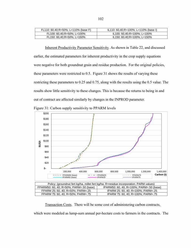
102
FL110: 60,40;R=50%; L=110% (base F) IL110: 60,40;R=100%; L=110% (base I) FL100: 60,40;R=50%; L=100% IL100: 60,40;R=100%; L=100% FL150: 60,40;R=50%; L=150% IL150: 60,40;R=100%; L=150%
Inherent Productivity Parameter Sensitivity. As shown in Table 22, and discussed
earlier, the estimated parameters for inherent productivity in the crop supply equations
were negative for both groundnut grain and residue production. For the original policies,
these parameters were restricted to 0.5. Figure 31 shows the results of varying these
restricting these parameters to 0.25 and 0.75, along with the results using the 0.5 value. The
results show little sensitivity to these changes. This is because the returns to being in and
out of contract are affected similarly by changes in the INPROD parameter.
Figure 31: Carbon supply sensitivity to PPARM levels
$-
$20
$40
$60
$80
$100
$120
$140
$160
$180
$200
- 200,000 400,000 600,000 800,000 1,000,000 1,200,000 1,400,000Carbon (t)
$US/
t
FPARM50 (base) FPARM25 FPARM75IPARM50 (base) IPARM25 IPARM75
Policy: (groundnut fert kg/ha, millet fert kg/ha; R=residue incorporation; PARM values)
FPARM50: 60, 40; R=50%; PARM=.50 (base) IPARM50: 60, 40; R=100%; PARM=.50 (base) FPARM 25: 60, 40; R=50%; PARM=.25 IPARM 25: 60, 40; R=100%; PARM=.25 FPARM 75: 60, 40; R=50%; PARM=.75 IPARM 75: 60, 40; R=100%; PARM=.75
Transaction Costs. There will be some cost of administering carbon contracts,
which were modeled as lump-sum annual per-hectare costs to farmers in the contracts. The

103
value used in the original policy analysis was 1000 CFA/ha, or $2 USD. Figure 32 and
Figure 33 show the sensitivity of the results to increasing this cost to $10 USD/ha. Series
“FT1”, representing the practice with 30 kg/ha fertilizer,50% residue incorporation and
$10/ha transaction costs, bends backwards because transactions costs are $0/ha when
carbon prices are $0/ha – when prices increase to $10 and $20/t, this is not enough to offset
the threshold created by the higher transaction cost. Higher transactions costs resulted in
lower participation rates and sequestration rates, particularly in the lower carbon price
ranges.
The results were particularly sensitive in the lower ranges. For example, at $20/t
Carbon, participation ranged from 15% to 41%. This shows that the cost efficiency of
potential carbon programs is important.
Figure 32: Carbon supply sensitivity to contract transaction costs
$-
$20
$40
$60
$80
$100
$120
$140
$160
$180
$200
- 200,000 400,000 600,000 800,000 1,000,000 1,200,000 1,400,000
Carbon (t)
$US/
t
F TC=$2 F TC=$10 I TC=$2 I TC=$10
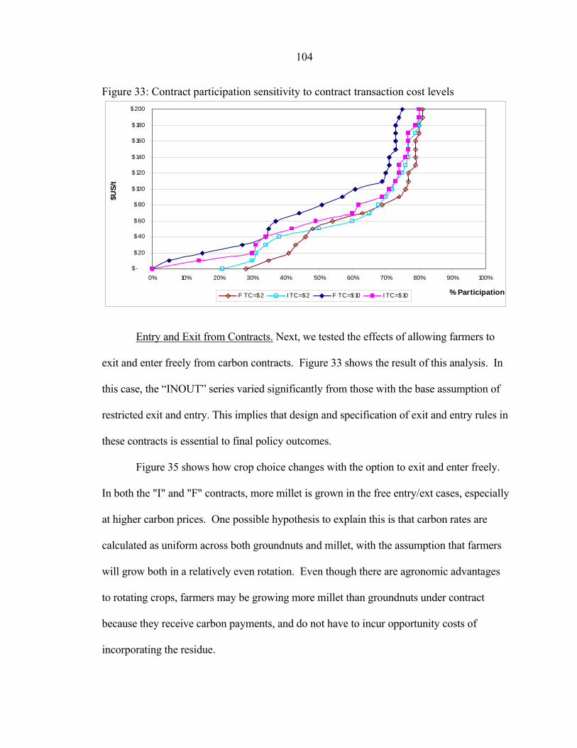
104
Figure 33: Contract participation sensitivity to contract transaction cost levels
$-
$20
$40
$60
$80
$100
$120
$140
$160
$180
$200
0% 10% 20% 30% 40% 50% 60% 70% 80% 90% 100%
% Participation
$US/
t
F TC=$2 I TC=$2 F TC=$10 I TC=$10
Entry and Exit from Contracts. Next, we tested the effects of allowing farmers to
exit and enter freely from carbon contracts. Figure 33 shows the result of this analysis. In
this case, the “INOUT” series varied significantly from those with the base assumption of
restricted exit and entry. This implies that design and specification of exit and entry rules in
these contracts is essential to final policy outcomes.
Figure 35 shows how crop choice changes with the option to exit and enter freely.
In both the "I" and "F" contracts, more millet is grown in the free entry/ext cases, especially
at higher carbon prices. One possible hypothesis to explain this is that carbon rates are
calculated as uniform across both groundnuts and millet, with the assumption that farmers
will grow both in a relatively even rotation. Even though there are agronomic advantages
to rotating crops, farmers may be growing more millet than groundnuts under contract
because they receive carbon payments, and do not have to incur opportunity costs of
incorporating the residue.

105
Figure 34: Participation sensitivity to entry and exit restrictions
$-
$20
$40
$60
$80
$100
$120
$140
$160
$180
$200
0% 10% 20% 30% 40% 50% 60% 70% 80% 90% 100%
Participation %
$US/
t
F INOUT_F I INOUT_I
Figure 35: Crop choice composition with and without entry/exit restrictions
$-
$20
$40
$60
$80
$100
$120
$140
$160
$180
$200
40% 42% 44% 46% 48% 50% 52% 54% 56% 58% 60%% of fields in groundnuts
$US/
t
F INOUT_F I INOUT_I
MORE MILLET MORE GROUNDNUTS
Fertilizer Response Functions. Figure 26 shows the fertilizer response function
imposed in the simulation model. In the sensitivity analysis we tested three different sets of
kink points for this function, for each crop. The base level used for most of the scenarios
was 69 kg/ha in groundnuts, and 48 kg/ha in millet. We also tested 90% and 120% of these

106
levels (62 and 43 kg/ha; 83 and 58 kg/ha) to see if this assumption affected the results.
Figure 36 shows the resultant participation levels, and Figure 37 show s the carbon supply
curves associated with contract "I" (60, 40 fertilizer; 100% residue). From these figures, it
is apparent that this specification has little impact on the results.
Figure 36: Contract "I" participation with 3 different fertilizer response functions (X6KINK)
$-
$20
$40
$60
$80
$100
$120
$140
$160
$180
$200
0% 10% 20% 30% 40% 50% 60% 70% 80% 90% 100%
% Participation
$US/
t
I: 69,48 kg/ha (base) I Kinks: 83,58 kg/ha I Kinks: 62,43 kg/ha

107
Figure 37: Carbon supply with 3 different fertilizer response functions (X6KINK)
$-
$20
$40
$60
$80
$100
$120
$140
$160
$180
$200
- 200,000 400,000 600,000 800,000 1,000,000 1,200,000 1,400,000
Carbon (t)
$US/
t
I Kinks: 62,43 kg/ha I Kinks: 83,58 kg/ha I Kinks: 69,48 kg/ha
Groundnut Residue Prices. Finally, we examined how groundnut residue prices
impacted the results. This price has the potential to increase with carbon sequestration
programs, for reasons of endogenaity discussed in Chapter 4. Figure 38 and Figure 39 show
how this price can impact the results substantially, particularly in the lower and
intermediate carbon price ranges. As expected, as this price rose, participation and carbon
supply shifted inwards.

108
Figure 38: Contract participation sensitivity to groundnut residue price (PB1C)
$-
$20
$40
$60
$80
$100
$120
$140
$160
$180
$200
0% 10% 20% 30% 40% 50% 60% 70% 80% 90% 100%Participation
$US/
t
IPB50 IPB150 IPB200 IPB250 I100 (base)
All "I" policies, requiring 60kg/ha, 40kg/ha (fert. on groundnuts, millet) and 100% residue incorp'n IPB50: Price(GN Residue) = 50% IPB150: Price(GN Residue) = 150% IPB200: Price(GN Residue) = 200% IPB250: Price(GN Residue) = 250% I100: Price(GN Residue) = 100% = Base "I" Simulation
Figure 39: Carbon supply sensitivity to groundnut residue price (PB1C)
$-
$20
$40
$60
$80
$100
$120
$140
$160
$180
$200
- 200,000 400,000 600,000 800,000 1,000,000 1,200,000 1,400,000
Carbon (t)
$US/
t
IPB50 IPB150 IPB200 IPB250 I100 (base)
All "I" policies, requiring 60kg/ha, 40kg/ha (fert. on groundnuts, millet) and 100% residue incorp'n IPB50: Price(GN Residue) = 50% IPB150: Price(GN Residue) = 150% IPB200: Price(GN Residue) = 200% IPB250: Price(GN Residue) = 250% I100: Price(GN Residue) = 100% = Base "I" Simulation

109
Discussion
From the sensitivity analysis, it is apparent that certain assumptions and variables
are highly influential on supply responses. For example, if groundnut residue prices
increase substantially for exogenous or endogenous reasons, this will cause adoption rates
(and therefore carbon sequestration rates) to be much lower at a given price level. Other
factors, such as entry and exit restrictions, costs of administering the program and
transactions costs can also impact participation and sequestration rates, particularly at lower
price levels.
Labor costs also play an important role in determining outcomes of policies. For
this reason, it is important that agronomists and economists effectively estimate the costs of
participating in the contract management practices, particularly the costs of incorporating
residue.
The results of this type of analysis can be used by policy makers to assess carbon
sequestration potential in Senegal's Groundnut Basin. World carbon prices, which will be
determined by the institutions and restrictions placed on polluters, are largely exogenous to
small countries like Senegal. For that reason, it is useful to see how much carbon
sequestering and storing services a region can supply, given a range of possible prices.
Policy "I", which required at least 60 kg/ha and 40 kg/ha fertilizer on groundnut and
millet fields, and 100% groundnut residue incorporation, was the only management regime
that could increase (or, for that matter, maintain) simulated SOC and inherent productivity
levels on a given field. For this reason, we are particularly interested in the simulated
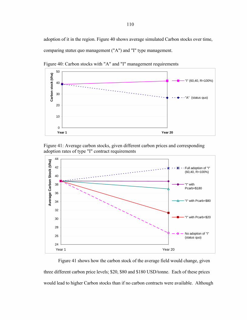
110
adoption of it in the region. Figure 40 shows average simulated Carbon stocks over time,
comparing status quo management ("A") and "I" type management.
Figure 40: Carbon stocks with "A" and "I" management requirements
0
10
20
30
40
50
Year 1 Year 20
Car
bon
stoc
k (t/
ha)
"I" (60,40, R=100%)
"A" (status quo)
Figure 41: Average carbon stocks, given different carbon prices and corresponding adoption rates of type "I" contract requirements
24
26
28
30
32
34
36
38
40
42
44
Year 1 Year 20
Ave
rage
Car
bon
Stoc
k (t/
ha)
Full adoption of "I"(60,40, R=100%)
"I" withPcarb=$180
"I" with Pcarb=$80
"I" with Pcarb=$20
No adoption of "I"(status quo)
Figure 41 shows how the carbon stock of the average field would change, given
three different carbon price levels; $20, $80 and $180 USD/tonne. Each of these prices
would lead to higher Carbon stocks than if no carbon contracts were available. Although

111
net carbon sequestration occurs at all prices with "I" contracts, only high prices (i.e. $180/t)
cause enough adoption to essentially stop SOC losses in the region.
Figure 42: Average inherent productivity, given three carbon prices and corresponding adoption rates of type "I" contract requirements
500
600
700
800
900
Year 1 Year 20
Aver
age
Inpr
od s
core
(est
imat
ed y
ield
kg/
ha)
Full adoption of"I" (60,40,R=100%)
"I" withPcarb=$180
"I" withPcarb=$80
"I" withPcarb=$20
No adoption of "I"(status quo)
Note: These inherent productivity scores are standardized to the same intercept, and averaged across fields
and between crops.
Carbon price levels would affect inherent productivity similarly. At all carbon
prices, offering carbon contract "I" would mitigate losses in land productivity. Given high
carbon prices, farmers could sustain, or even increase the inherent productivity of their
fields. Figure 42 shows these effects.

112
CHAPTER 6
CONCLUSION
Human induced soil degradation has multiple forms, including: nutrient decline,
erosion, salinization and physical compaction (ISRIC GLASOD, 2004). In Sudo-Sahelian
Africa, erosion and nutrient mining are prominent causes of soil degradation. Nutrient
mining occurs when more nutrients, such as nitrogen, phosphorus, potassium, carbon, and
micronutrients, are removed from the soil than are put back into the system. In the case of
Senegal, harvesting grains and crop residue from the land impact heavily on soil carbon
content, while insufficient replacement of soil nutrients with fertilizers leads to negative
nutrient balances. Policies that encourage or enable farmers to incorporate crop residues
into their soils, and to increase mineral fertilizer usage, would help to reduce or reverse
these types of soil degradation in the region.
Given the economic perspective of the rational farmer and the dynamic nature of
crop and soil management issues, this thesis used a regional case study in the Groundnut
Basin of Senegal to do the following: describe and assess economic incentives specific the
to the case study region; model the farmer's production and decision making process;
design carbon contract policies and model them within the farmer’s decision making
process; simulate the interaction between the current agricultural marketplace and the new
carbon policies; and to assess the role that carbon sequestration could play in helping the

113
region deal with soil degradation problems, if and when international action is taken to
reduce greenhouse gas emissions.
In Chapters 2 and 4, we hypothesized that farmers are using insufficient quantities
of fertilizers for several reasons. Information from farmers in the region indicates that
several factors constrain fertilizer use, including financial constraints and market
imperfections. The result of these constraints is to reduce the productivity and increase the
farm gate cost of fertilizers. The results of the simulation supported this hypothesis. The
carbon contracts that were simulated allowed farmers unrestricted access to fertilizer at
market prices. Even when carbon prices were $0/tonne, farmers still participated in
contracts, and used more fertilizer than they would have in a status quo environment.
The larger question that this thesis attempted to address was: can payments for
carbon sequestration services mitigate and/or reverse soil degradation trends in this region?
Using data from the Groundnut Basin in Senegal, and employing an econometric-
process simulation model, this study found that some carbon contracts could be used to
reduce losses in soil carbon and productivity; however, only the most intensive
management policy “I” resulted in sustained carbon stocks and simulated productivity
levels, and that only occurred at high Carbon prices ($180 USD/t carbon and higher).
Furthermore, the adoption of this practice, which requires farmers to incorporate at least 60
kg/ha of fertilizer in groundnut fields, 40 kg/ha in millet fields, 100% of groundnut residues
into the soil, was found to be sensitive to the assumptions maintained in the analysis. For
example, if groundnut residue prices, contract monitoring transactions costs, or labor costs
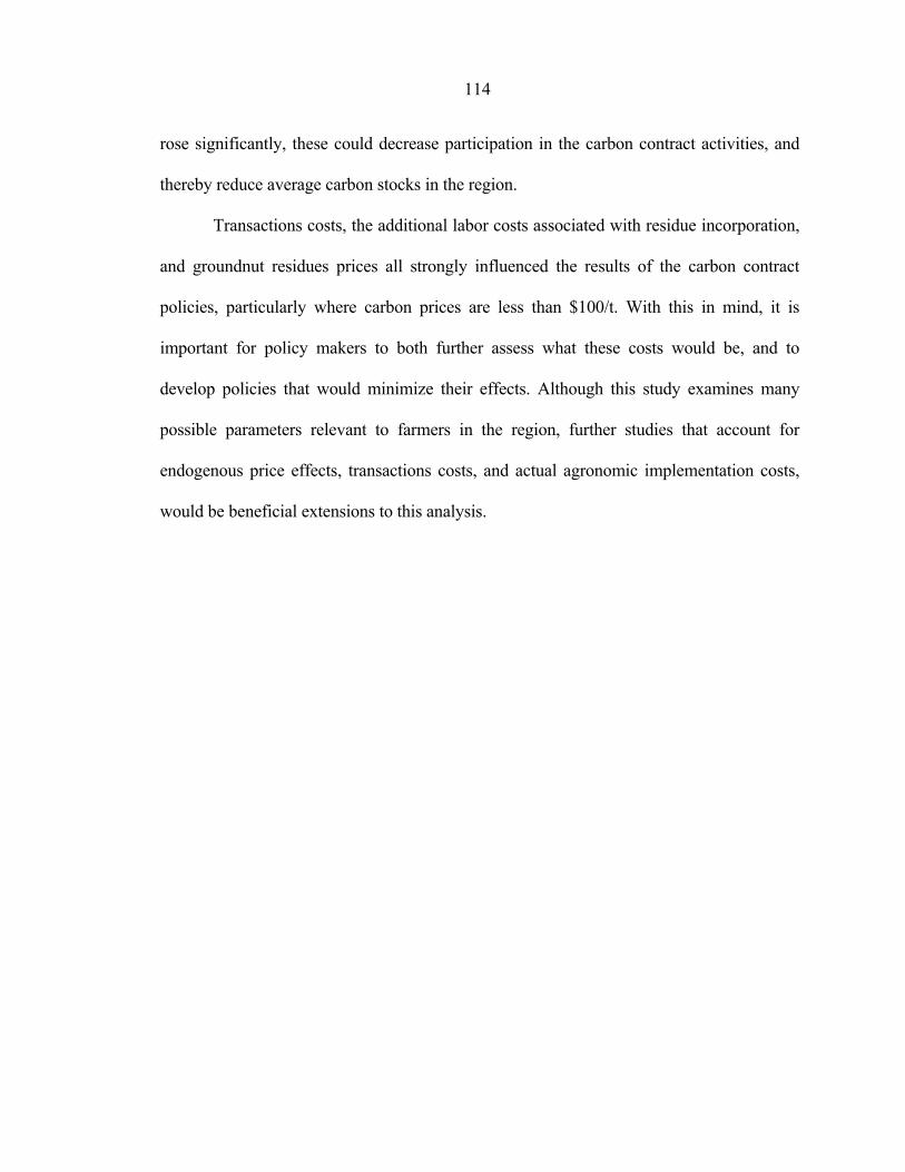
114
rose significantly, these could decrease participation in the carbon contract activities, and
thereby reduce average carbon stocks in the region.
Transactions costs, the additional labor costs associated with residue incorporation,
and groundnut residues prices all strongly influenced the results of the carbon contract
policies, particularly where carbon prices are less than $100/t. With this in mind, it is
important for policy makers to both further assess what these costs would be, and to
develop policies that would minimize their effects. Although this study examines many
possible parameters relevant to farmers in the region, further studies that account for
endogenous price effects, transactions costs, and actual agronomic implementation costs,
would be beneficial extensions to this analysis.

115
BIBLIOGRAPHY
Akobundu, E. 1998. "Farm-Household Analysis of Policies Affecting Groundnut Production in Senegal." Virginia Polytechnic Institute and State University.
Allard, C., A. D'Hoore, N. Le, L. Moers, and J. Wiegand. 2003. "Statistical Annex." International Monetary Fund.
Antle, J. M. and B. Diagana. 2003. "Creating Incentives for the adoption of sustainable agricultural practices in developing countries; The role of soil carbon sequestration." American Journal of Agricultural Economics, 85, pp. 1178-84.
Antle, J. M. and L. M. Young. 2003. "Policies and Incentive Mechanisms for the Permanent Adoption of Agricultural Carbon Sequestration Practices in Industrialized and Developing Countries." Paper presented at the Climate Change, Carbon Dynamics and World Food Security conference, The Ohio State University, Columbus, Ohio, USA, June 10–11.
Antle, J. M. and S.M. Capalbo. 2001. "Agriculture as a Managed Ecosystem: Policy Implications." Journal of Agricultural and Resources Economics.
Antle, J.M and J. Stoorvogel. 2001. "Integrating Site-Specific Biophysical and Economic Models to Assess Trade-Offs in Sustainable Land Use and Soil Quality," in Economic policy and sustainable land use: Recent advances in quantitative analysis for developing countries. Nico Heerink, Herman van Keulen and Marijke eds Kuiper eds. Antle, J.M and SM Capalbo. 2001. "Econometric-Process Models for Integrated Assessment of Agricultural Production Systems." American Journal of Agricultural Economics, 83:2, pp. 389-401.
Antle, J.M., S.M. Capalbo, S. Mooney, E.T. Elliott and K.H. Paustian. 2001. "Economic Analysis of Agricultural Soil Carbon Sequestration: An Integrated Assessment Approach." Journal of Agricultural and Resource Economics, 26:2, pp. 344-67.
Antle, J.M., S.M. Capalbo, S. Mooney, E.T. Elliott, and K.H. Paustian. 2003. “Spatial Heterogeneity, Contract Design, and the Efficiency of Carbon Sequestration Policies for Agriculture.” Journal of Environmental Economics and Management, 46(2):231-250.
Ba, M., M. Mbaye, S. Ndao, A. Wade, and L. Ndiaye. 2000. "Région de Diourbel: Cartographie des changements dans l'occupation-l'utilisation du sol dans le Centre-Ouest du Sénégal." Rapports entre les politiques gouvernementales et les investissements paysans en Afrique semi-aride: Série Sénégal: 32. Drylands Research: Crewkerne, Somerset.

116
Bachelier, M. 2004. "PERC Report Vol 22 No. 2 Special Issue: Africa." PERC Reports. The Property and Environment Research Center, Bozeman, Montana.
Badiane, C. 2001. Senegal's Trade in Groundnuts: Economic, Social and Environmental Implications, TED Case Studies: Number 646, December 2001. Available at http://www.american.edu/TED/senegal-groundnut.htm.
Ballantyne, B., M.Bristow, B. Davison, S. Harrington, and K. Khan. 2000. "How Can Land Tenure and Cadastral Reform Succeed? An Inter-Regional Comparison of Rural Reforms." Canadian Journal of Development Studies, 21:3, pp. 693-723.
Barry, A., Ndiaye, S., Ndiaye, F., and Tiffen, M. 2000. 'Région de Diourbel: Les aspects démographiques', Drylands Research Working Paper 13. Drylands Research, Crewkerne, United Kingdom.
Bationo, A., Lompo, F., Koala, S., 1998. "Research on nutrient flows and balances in West Africa: state-of-the-art." Agriculture, Ecosystems and Environment 71 (1–3), 19–35.
Boserup, E.. 1965. The Conditions of Agricultural Growth: The Economics of Agricultural Change Under Population Pressure, Chicago: Aldine.
Bouma, J., N.H. Batjes, and J.J.R. Groot. 1998. "Exploring land quality effects on world food supply." Geoderma, 86, pp. 43-59.
Breman, H., J.J.R. Groot, and H. van Keulen. 2001. "Resource limitation in Sahelian agriculture." Global Environmental Change, 11, pp. 59-68.
Breman, H., Uithol, P.W.J. 1984. The Primary Production in the Sahel (PPS) Project—A ‘Bird’s-Eye View. Centre for Agrobiological Research, Wageningen.
Cour, J.M.. 2000. "The Sahel in West Africa: countries in transition to a full market economy." Global Environmental Change, 11, pp. 31-47.
de Jager, A. 2005. "Participatory technology, policy and institutional development to address soil fertility degradation in Africa." Land Use Policy, 22:1.
de Jager, A., A.U. Mokwunye, and E.M.A. Smaling. 1998. "Do Fertilizers Play a Major Role in Sustainable Agricultural Development in West Africa?" in Economics of agro-chemicals: An international overview of use patterns, technical and institutional determinants, policies and perspectives: Selected papers of the symposium of the International Association of Agricultural Economists held at Wageningen, the Netherlands, 24-8, April 1996. A. Grada, A. Wossink, Gerrit C. van Kooten and George H. Peters eds.
117
de Willigen, P., L. Bergstrom, and R.G. Gerritse. 1990. “Leaching Models of the Unsaturated Zone, Their Potential Use for Management and Planning.” In Proceedings of The International Symposium on Water Quality Modeling of Agricultural Non-point Sources, ed., D.G. Decoursey, pp. 105–28. Washington, DC: U.S. Department of Agriculture.
Delgado, C. L., J. Hopkins, and V. A. Kelly. 1998. Agricultural growth linkages in sub-Saharan Africa. With Peter Hazell et al. Research Report 107. Washington, D.C.: International Food Policy Research Institute.
Diagana, B. 2003. Land Degradation in Sub Saharan Africa (SSA): What Explains the Widespread Adoption of Unsustainable Farming Practices? Draft working paper, Department of Agricultural Economics and Economics, Montana State University, Bozeman, MT, USA, June.
Diagana, B. and F. Akindes, K. Savadogo, T. Reardon, and J. Staatz.1999. "Effects of the CFA Franc Devaluation on Urban Food Consumption in West Africa: Overview and Cross-Country Comparisons." Food Policy, 24:5, pp. 465-78.
Diagana, B. and T. Reardon. 1999. "Household Consumption Responses to the Franc CFA Devaluation: Evidence from Urban Senegal." Food Policy, 24:5, pp. 495-515.
Diop, N., J. Beghin, and M. Sewadeh. 2004. "Groundnut Policies, Global Trade Dynamics, and the Impact of Trade Liberalization." The World Bank, Policy Research Working Paper Series.
Donovan, G. and F. Casey. 1998. "Soil fertility management in Sub-Saharan Africa." World Bank technical paper: 67. The World Bank: Washington, D.C.
Drechsel, P., L. Gyiele, D. Kunze, and O. Cofie. 2001. "Population density, soil nutrient depletion, and economic growth in sub-Saharan Africa." Ecological Economics, 38, pp. 251-58.
Economic Research Service. 2004. Food Security Assessment: GFA-15. Washington, DC: U.S. Department of Agriculture.
Ehrlich, P.R. 1968. The Population Bomb, New York: Ballantine Books.
English, J., M. Tiffen, and M. Mortimore. 1994. Land resource management in Machakos District, Kenya, 1930-1990: Environment Paper, no. 5. Washington, D.C.: World Bank.

118
Enyong, L. A., S. K. Debrah, and A. Bationo. 1999. "Farmers' perceptions and attitudes towards introduced soil-fertility enhancing technologies in western Africa." (Nutrient Cycling in Agroecosystems), 53:2, pp. 177.
Fall, W.W. 2001. "Région de Diourbel: The Family, Local Institutions and Education ", Drylands Research Working Paper 20. Drylands Research, Crewkerne, United Kingdom.
FAO/WFP. 2002. Crop and food supply Assessment mission to Senegal. FAO. Rome.
Faye, A., Fall, A., Tiffen,M., Mortimore, M., Nelson, J. 2001. "Région de Diourbel: Synthesis", Drylands Research Working Paper 23a. Drylands Research, Crewkerne, United Kingdom.
Feng, H, L.A. Kurkalova, C.L. Kling, and P.W. Gassman. 2004. "Environmental conservation in Agriculture: Land Retirement versus Changing Practices on Working Land." Center for Agricultural and Rural Development.
Fernandes, P., R. Oliver, and S. Diatta. 2000. "Changes in Organic Matter of a Ferrallitic Tropical Soil Degraded by Cropping Systems: The Case of Southern Senegal." Arid Soil Research and Rehabilitation, 14, pp. 137-50.
Ghadiri, H., and C.W. Rose. 1992. Modeling Chemical Transport in Soils. Boca Raton, FL: Lewis Publishers.
Gijsman, A. J., G. Hoogenboom, W. J. Parton, and P. C. Kerridge. 2002. "Modifring DSSAT Crop Models for Low-Input Agricultural Systems Using a Soil OrganicMatter-Residue Module from CENTURY." Agronomy Journal, 94.
Goetz, S. J. 1992. "Economies of Scope and the Cash Crop-Food Crop Debate in Senegal." World Development, 20 No. 5, pp. 727-34.
Golan, E. H. 1994. "Sustainability and Migration: Experiments from the Senegalese Peanut Basin." Annals of Regional Science, 28:1, pp. 91-106.
Goldsmith, P. D., K. Gunjal, and B. Ndarishikanye. 2004. "Rural-Urban Migration and Agricultural Productivity: The Case of Senegal." Agricultural Economics, 31:1, pp. 33-45.
Grigsby, W. J. 2002. "Subsistence and Land Tenure in the Sahel." Agriculture and Human Values, 19:2, pp. 151-64.
Hammer, J.S. 1986. "'Subsistence First': Farm Allocation Decisions in Senegal." Journal of Development Economics, 23:2, pp. 355-69.

119
Harsch, E. 2003. "Senegal: to fight hunger, modernize farming - an uncertain path amidst conflicting interests and pressures." Africa Recovery, Vol. 17: 14.
Hathie, I. and R.A. Lopez. 2002. "The Impact of Market Reforms on the Senegalese Peanut Economy." Journal of International Development, 14:5, pp. 543-54.
Heath, J. and H. Binswanger. 1996. "Natural Resource Degradation Effects of Poverty and Population Growth Are Largely Policy-Induced: The Case of Colombia." Environment and Development Economics, 1:1, pp. 65-84.
Heerink, N. 2005. "Soil Fertility decline and economic policy reform in Sub-Saharan Africa." Land Use Policy, 22:1.
Heisey, P.W. and W. Mwangi. 1996. "Fertilizer Use and Maize Production in Sub-Saharan Africa." CIMMYT Economics Working Paper 96-01.
Hunt, H.W., M.J. Trlica, E.F. Redente, J.C. Moore, J.K. Detling, T.G.F. Kittel, D.E. Walter, M.C. Fowler, D.A. Klein, and E.T. Elliott. 1991. “Simulation Model for the Effects of Climate Change on Temperate Grassland Ecosystems.” Ecol. Model. 53:205– 46.
IFDC. 2002. "Africa Fertilizer Situation." Market Information Unit; Market Development Division: FSR-1. Muscle Shoals, Alabama.
IIED. 1999. "Land Tenure and Resource access in West Africa: Issues and opportunities for the next twenty five years." International Institute for Environment and Development.
Ingram, J.S.I., and E.C.M. Fernandes. 2001. “Managing Carbon Sequestration in Soils: Concepts and Terminology.” Agriculture, Ecosystems and Environment 87:111–17.
IPCC. 2001. Climate change 2001: synthesis report. Cambridge University Press, Cambridge.
Johnson, S.R. and G.C. Rausser. 2001. "Effects of Misspecifications of Log-Linear Functions When Sample Values are Zero or Negative."
Juo, A.S.R., Kang, B.T. 1989. Nutrient effects of modification of shifting cultivation in West Africa. In: Proctor, J. (Ed.), Mineral Nutrients in Tropical Forest and Savanna Ecosystems. Blackwell, Oxford, pp. 289–300.
Kelly, V., A. A. Adesina, and A. Gordon. 2003. "Expanding access to agricultural inputs in Africa: a review of recent market development experiences." Food Policy, 28:379-404.

120
Kelly, V., B. Diagana, T. Reardon, M. Gaye, and E. Crawford. 1996. "Cash Crop and Foodgrain Productivity in Senegal: Historical View, New Survey Evidence, and Policy Implications." MSU International Development Papers. Michigan State University.
Kherallah, M., C. Delgado, E. Gabre-Madhin, N. Minot, and M. Johnson. 2000. "Agricultural Market Reforms in Sub-Saharan Africa: A Synthesis of Research Findings." 263. International Food Policy Research Institute: Washington D.C.
Kim, K.S. 2003. "Development Crisis in Sub-Sahel Africa: Globalization, Adjustment, and Roles of International Institutions." University of Notre Dame.
Kiome, R.M. and M. Stocking. 1995. "Rationality of farmer perception of soil erosion: the effectiveness of soil conservation in semi-arid Kenya". Global Environmental Change: Human and Policy Dimensions 5(4): 281-95.
Koning, N. and E. Smaling. 2005. "Environmental crisis or 'lie of the land'? The debate on soil degradation in Africa." Land Use Policy, 22:1, pp. 1-9.
Lal, R. 2004. "Soil Carbon Sequestration Impacts on Global Climate Change and Food Security." Science, 304:June, pp. 1623-27.
Lal, R. 2004. "Supplemental Online Material for Soil Carbon Sequestration Impacts on Global Climate Change and Food Security." Science, Vol. 304.
Lal, R., M. Griffin, J. Apt, L. Lave, and M. G. Morgan. 2004. "Managing Soil Carbon." Science, Vol. 304: 393.
Lutz, E., S. Pagiola, and C. Reiche. 1994. "The Costs and Benefits of Soil Conservation: The Farmers' Viewpoint." World Bank Research Observer, 9:2, pp. 273-95.
Malthus, T. 1798. An essay on the principle of population as it affects the Future Improvement of Society. London: Ward Lock.
McCarl, B.A., and U.A. Schneider. 2001. “The Cost of Greenhouse Gas Mitigation in U.S. Agriculture and Forestry.” Science 294(December 21): 2481-2482.
Meadows, D. H., D.L. Meadows, J. Randers, and W. Behrens. 1972. The Limits to Growth: A Report for the Club of Rome´s Project on the Predicament of Mankind. New York: Signet.
Metcalfe, L. 2003. "Nationmaster." Vol. 2004: Country data website. Rapid Intelligence Pty Ltd: Sydney.
Mortimore, M. and F. Harris. 2005. "Do small farmers' achievements contradict the nutrient depletion scenarios for Africa?" Land Use Policy, 22:1.

121
Mortimore, M. and M. Tiffen. 2004. "Introducing Research into Policy: Lessons from District Studies of Dryland Development in Sub-Saharan Africa." Development Policy Review, 22:3, pp. 259-85.
Mortimore, M. J. and W.M. Adams. 2000. "Farmer adaptation, change and 'crisis' in the Sahel." Global Environmental Change, 11, pp. 49-57.
Moseley, W. G. 2001. "African Evidence on the relation of poverty, time preference and the environment." Ecological Economics, 38, pp. 317-26.
Ndoye, O. 1992. "An Economic Analysis of Factors Affecting Millet Production and Transactions in the Peanut Basis of Senegal." Michigan State University.
Niang, A. 2004. "Organic matter stocks under different types of land use in the Peanut Basin of the Nioro area, Senegal." Department of Environmental Sciences. Wageningen University.
Niemeijer, D. and M. Valentina. 2002. "Soil Degradation in the West African Sahel How Serious Is It?" Environment, 44:2, pp. 12.
Oldeman, L. R., R. T. A. Hakkeling, and W. G. Sombroek. 1990. "World Map of the Status of Human-Induced Soil Degradation; Explanatory Note." ISRIC and UNEP.
Parton, W.J., D.S. Schimel, D.S. Ojima, and C.V. Cole. 1994. “A General Model for Soil Organic Matter Dynamics: Sensitivity to Litter Chemistry, Texture and Management.” In Quantitative Modeling of Soil Forming Processes, SSSA Special Publication 39, eds., R.B. Bryant and R.W. Arnold, pp. 147–67. Madison, WI: Soil Science Society of America.
Paustian, K. 1994. “Modelling Soil Biology and Biogeochemical Processes for Sustainable Agriculture Research.” In Management of Soil Biota in Sustainable Farming Systems, 30 eds., C. Pankhurst, B.M. Doube, V.V.S.R. Gupta, and P.R. Grace, pp. 182–96. Melbourne: CSIRO Publishing.
Pautsch, G.R., L.A. Kurkalova, B.A. Babcock, and C.L. Kling. 2001. “The Efficiency of Sequestering Carbon in Agricultural Soils.” Contemporary Economic Policy, 19(2): 123-134.
Perry, D. 2000. "Rural weekly markets and the dynamics of time, space and community in Senegal." The Jounal of Modern African Studies, pp. 461-86.
Pieri, C. 1989. Fertilite des terres de Savanes: bilan de trente ans de recherche et de developpement agricoles au sud du Sahara. Ministere de Cooperation et du Developpement, Paris.

122
Reardon, T., Barrett, C., Kelly, V., Savadogo, K. 1999. "Policy reforms and sustainable agricultural intensification in Africa." Development Policy Review 17 (4), 375–395.
Ritchie, J.T. 1994.“Classification of Crop Simulation Models.” In Crop Modeling and Related Environmental Data: A Focus on Applications for Arid and Semiarid Regions in Developing Countries, Monograph Series, Vol. 1, eds., P.F. Uhlir and G.C. Carter, pp. 3–14, Paris: CODATA Commission on Global Change.
Rosen, C. J., P. M. Bierman, and R. D. Eliason. 1998. "Soil Test Interpretations and Fertilizer Management for Lawns, Turf, Gardens, and Landscape Plants." Vol. 2004. University of Minnesota Extension Service.
Sanchez, P. A. 2002. "Soil fertility and hunger in Africa." Science, 295:5562, pp. 2019.
Scherr, S. J. 1999. Soil degradation: A threat to developing-country food security by 2020? Food, Agriculture, and the Environment Discussion Paper 27. Washington, D.C.: International Food Policy Research Institute.
Scoones, I., 1997. The dynamics of soil fertility change; historical perspectives on environmental transformation from Zimbabwe. Geographical Journal 163 (2), 161–169
Simon, J.L. 1986. Theory of Population and Economic Growth. Basil Blackwell, Oxford.
Soil Management CRSP. 2002. A Soil Carbon Accounting and Management System for Emissions Trading. Special Publication SM CRSP 2002-04, Soil Management Collaborative Research Support Program, University of Hawaii, Honolulu, Hawaii, pp. 69–98.
Soufi, W. 2001. Agricultural research in Senegal: Economic surplus evaluation of the adoption of variety La Fleur 11 by peanut farmers. M.S. Thesis, Virginia Tech.
Soorvogel, J.J. and E.M.A. Smaling. 1990. "Assessment of soil nutrient depletion in Sub-Saharan Africa." The Winand Staring Centre.
Stoorvogel, J.J., J.M. Antle, C.C. Crissman, and W. Bowen. 2001. The Tradeoff Analysis Model Version 3.1: A Policy Decision Support System for Agriculture – User Guide. Laboratory of Soil Science and Geology, Wageningen University, The Netherlands.
Stoorvogel, J., J.M. Antle, C. Crissman, and W. Bowen. 2002. "The Tradeoff Analysis Model: Integrated Bio-physical and Economic Modeling of Agricultural Production Systems." Montana State University.
123
Swift, M.J., P.D.Seward, P.G.H. Frost., J.N.Qureshi, and F.N. Muchena. 1994. Long-term experiments in Africa: developing a database for sustainable land use under global change. In: Leigh, F.A., Johnston, A.E. (Eds.), Long-term Experiments in Agricultural and Ecological Sciences. CAB International, Wallingford, pp. 229–251.
Templeton, S.R., and S.J. Scherr. 1999. "Effects of demographic and related microeconomic change on land quality in hills and mountains of developing countries." World Development 27 (6), 903–918.
Thornton, P. K., and M. Herrero. 2001. Integrated crop-livestock simulation models for scenario analysis and impact assessment. Agricultural Systems 70(2-3):581-602.
Tiffen, M. 2003. "Transition in Sub-Saharan Africa: Agriculture, Urbanization and Income Growth”. World Development 31(8), 1343-1366.
Tiffen, M. and M. Mortimore. 1997. "Environment, Population Growth and Productivity in Kenya: A Case Study of Machakos District," in The economics of population: Key modern writings. Volume 2. Julian L. Simon ed.
Tiffen, M. M. Mortimore, and F. Gichuki. 1994. More People, Less Erosion: Environmental Recovery in Kenya. Wiley, London.
Tiffen, M., M. Mortimore, and F. Gichuki. 1994. "Population Growth and Environmental Recovery." International Institute for Environment and Development, Gatekeeper Series No. 45.
Tschakert, P. 2001. "Human Dimensions of carbon sequestration: A political ecology approach to soil fertility management and desertification control in the Old Peanut Basin of Senegal." Arid Lands, No. 49.
Tschakert, P. 2004. "The costs of soil carbon sequestration: an economic analysis for small-scale farming systems in Senegal." Agricultural Systems, 81.
UNAIDS/WHO. 2003. "AIDS Epidemic Update." Joint United Nations Programme on HIV/AIDS (UNAIDS), World Health Organization (WHO), Geneva, Switzerland. Available at: http://www.who.int/hiv/pub/epidemiology/epi2003/en/.
UNFCCC. “Issues in the Negotiating Process: Land Use, Land Use Change and Forestry Under the Kyoto Protocol.” Available at http://unfccc.int/issues/lulucf.html. 2004.
Valdivia, R.O. 2002. The Economics of Terraces in the Peruvian Andes: An Application of Sensitivity Analysis in an Integrated Assessment Model. Thesis, Master of Sciences in Applied Economics, Montana State University-Bozeman, USA.

124
Warning, M. and E. Sadoulet. 1998. "The Performance of Village Intermediaries in Rural Credit Delivery under Changing Penalty Regimes: Evidence from Senegal." Journal of Development Studies, 35:1, pp. 115-38.
Watson, R.T., I.R. Noble, B. Bolin, N.H. Ravindranath, D.J. Verardo, and D.J. Dokken. 2000. Land Use, Land-Use Change, and Forestry, A special report of the IPCC, Cambridge University Press, Cambridge, England.
Whisler, F.D., B. Babcock, D.N. Baker, R.E. Fye, H.F. Hodges, J.R. Lambert, H.E. Lemmon, J.M. McKinion, and V.R. Reddy.1986. “Crop Simulation Models in Agronomic Systems.” Advances in Agronomy 40:141–208.
WHO. 2004. Core Health Indicators from the latest World Health Report. World Health Organization Statistical Information System (WHOSIS). Available at http://www3.who.int/whosis/country/indicators.cfm?country=sen.
Wood, E.C., G.G. Tappan, and A. Hadj. 2004. "Understanding the drivers of agricultural land use change in south-central Senegal." Journal of Arid Environments, 59: 565-82.
World Gazetteer. 2004. Population Data. Available at http://www.world-gazetteer.com/.