VOLUME 22 JOURNAL OF CLIMATE 15 SEPTEMBER 2009

Changing Frequency and Intensity of Rainfall Extremes over India from 1951 to 2003

CHANDRA KIRAN B. KRISHNAMURTHY

School of International and Public Affairs, Columbia University, New York, New York

UPMANU LALL

Department of Earth and Environmental Engineering, Columbia University, New York, New York

HYUN-HAN KWON

Water Resources Division, Korea Institute of Construction Technology, Gyeonggi-do, South Korea

(Manuscript received 17 October 2008, in final form 6 February 2009)

ABSTRACT

Using a 1951-2003 gridded daily rainfall dataset for India, the authors assess trends in the intensity and frequency of exceedance of thresholds derived from the 90th and the 99th percentile of daily rainfall. A nonparametric method is used to test for monotonic trends at each location. A field significance test is also applied at the national level to assess whether the individual trends identified could occur by chance in an analysis of the large number of time series analyzed. Statistically significant increasing trends in extremes of rainfall are identified over many parts of India, consistent with the indications from climate change models and the hypothesis that the hydrological cycle will intensify as the planet warms. Specifically, for the exceedance of the 99th percentile of daily rainfall, all locations where a significant increasing trend in frequency of exceedance is identified also exhibit a significant trend in rainfall intensity. However, extreme precipitation frequency over many parts of India also appears to exhibit a decreasing trend, especially for the exceedance of the 90th percentile of daily rainfall. Predominantly increasing trends in the intensity of extreme rainfall are observed for both exceedance thresholds.

1. Introduction

Anthropogenic climate change poses potentially sig­nificant risks for the Indian Subcontinent through changes in extreme rainfall characteristics. General circulation models ( G C M s ) of climate have had only limited success in reproducing the key attributes of the intraseasonal and interannual variations in the Indian monsoon. Conse­quently, it is not clear whether GCM simulations forced with the Intergovernmental Panel on Climate Change (IPCC)-style anthropogenic change scenarios adequately represent changes in Indian rainfall extremes, especially for extreme rainfall that translates into floods or for multiday dry periods that impact crop yield. Recently, a few papers (Guhathakurta and Rajeevan 2008; Goswami

et al. 2006) have investigated the trends in selected ex­treme rainfall attributes from a daily rainfall dataset that has become available through the Indian Meteo­rological Department ( I M D ) . Such analyses provide a useful backdrop for assessing whether forced GCM simulations, such as those by M a y (2004), Kumar et al. (2006), among others, provide plausible scenarios for changes in extreme rainfall in the twenty-first century.

This paper presents an exploratory, spatially dis­tributed analysis of the nature of monotonic trends in selected statistics of daily rainfall across India. The re­search presented differs from recent work on the issue (Goswami et al. 2006; Guhathakurta and Rajeevan 2008; Joshi and Rajeevan 2006; Rajeevan et al. 2008; Alexander et al . 2006; K l e i n Tank et al. 2006; Kumar et al. 2006; M a y 2004) in the specific statistics (frequency and intensity) of extremes considered, in the use of a nonparametric monotonie trend analysis (instead of a linear trend analysis, which is nonrobust to outliers, a concern in analyzing data on extremes), and in analyzing

Corresponding author address: Chandra Kiran B. Krishnamurthy, Columbia University. 918 S.W. Mudd Building, Mail Code 4711, 500 W. 120th St., New York, NY 10027. E-mail: cb2322@columbia.edu

DOI: 10.1175/2009JCLI2896.1

© 2009 American Meteorological Society 4737

4738 JOURNAL OF CLIMATE VOLUME 22

the complete spatially distributed dataset instead of an aggregate region. Further, we use methods for field sig­nificance analysis of spatial trends in each statistic and also document the concordance of trends across vari­ables. Trends in the frequency with which daily rainfall exceeds selected thresholds, as well as in the intensity (magnitude of such rainfall events) are considered at each grid cell over India. The rainfall amount considered to define the exceedance events corresponds to fixed per­centiles of the long-term rainfall data at that grid cell; hence, the threshold magnitude varies from grid cell to grid cell. Thus, changes in the local climatology of extremes, rather than the rate of occurrence of a fixed extreme magnitude across a region or even the entire country, are explored.

Further, analyzing trends in frequency and intensity separately is of interest since it is possible that the number of extreme events could increase without a correspond­ing increase in the intensity of each event (Trenberth 1999), and each measure provides information regarding different aspects of extreme rainfall. For instance, rainfall­-indexed insurance is being introduced by several organi­zations in India (Gine et al. 2007) and the determination of a fair premium, and the associated payout structure, requires an assessment of whether the upper tail of the probability distribution of daily rainfall is changing at the specific location where contracts are likely to be written. The need to inform these and similar applications moti­vates our spatially distributed analysis of trends in the exceedance of specific percentiles of the local distribution of daily rainfall.

In the monsoonal setting (Indian or As i an monsoon), there have been a few studies focused exclusively on trends in extreme rainfall and most of these have been based on greenhouse-gas-forced model-based scenarios of the IPCC for the twenty-first century (Lal et al. 2000; Bhaskaran and Mi tche l l 1998; M a y 2004; Kumar et al. 2006). Keeping in mind the biases in the models (indi­cated in Kumar et al. 2006), we note that most models appear to predict enhanced summer monsoonal pre­cipitation over parts of northwestern India, while pre­dicting little or no change over much of peninsular India (Kumar et al. 2006). Climate-model-based studies ap­pear to indicate an increase in the geographic extent of intense events but not necessarily an intensification of extreme events in areas already subject to high rainfall [which tend to be along the southwestern coast or the northeastern sub-Himalayan region (Kumar et al. 2006)]. M o d e l results also indicate intensification of rainfall in most of India except parts of central and northeastern India (May 2004), with the most intense (maximum 24-h rainfall) rainfall events predicted to occur over north­eastern and northwestern India.

The study by Goswami et al. (2006), using the same gridded dataset as here, reports an increasing trend in the frequency of extreme precipitation events, defined as events exceeding the thresholds of 100 and 150 mm, using pooled data from all grid cells over the central Indian region (the so-called monsoon belt), and also indicates an increase in the intensity of precipitation, as measured by the raw values of the 99.5th and 99.75th percentile of the rainfall distribution, over the same region.

Joshi and Rajeevan (2006) use station data (about 199 stations from 1901 to 2000) for India to carry out a linear, parametric trend analysis on various measures of extremes. They find increasing trends for certain regions (west coast and northwestern India) as well as an in­crease (as in Goswami et al . 2006) in the contribution of heaviest rains to total rainfall. Final ly , Rajeevan et al. (2008), using a longer station-level dataset (1901-2004), carry out an analysis very similar to Goswami et al. , over a slightly different region, and find increasing trends (after accounting for interdecadal variations in the ex­treme events) in both heavy and very heavy rainfall events (as defined in Goswami et al. 2006). They also make a preliminary attempt at l inking such trends to ocean surface temperatures.

a. Data

This study utilizes a recently available gridded daily dataset for India (Rajeevan et al. 2006), consisting of 1300 grid cells, each 1° latitude × 1° longitude, for 53 years (1951-2003), available from the I M D . O f these 1300 grids, 357 grids covering all of India's land area were used for the analysis. This is the same dataset from which Goswami et al. (2006) draw their subset for analysis.

b. Definition of statistics of extremes

W e consider two measures of extremes, frequency and intensity, defined, respectively, as the number of days with rainfall events (each year) exceeding a threshold and the average daily rainfall (for each year) on the days on which rainfall exceeds the specific threshold.

A threshold is defined in terms of a fixed percentile (two were considered: the 90th and the 99th) of the daily rainfall series at the grid cell , considering only days with nonzero rainfall. A s a result, the threshold magnitude varies from grid cell to grid cell (but not year to year). A time series of frequency at each grid cell is computed as

where t is the year, j the grid box, Pitj the rain on day i in year t at grid j, and P*

j is the rainfall threshold for grid j;

15 SEPTEMBER 2009 KRISHNAMURTHY ET AL. 4739

FIG. 1. Contours of exceedance thresholds of daily rainfall (mm) at each grid. The boxed area indicates the region considered in Goswami et al. (2006).

F is an indicator function that takes the value 1 if the argument is true and 0 otherwise.

Correspondingly, the intensity time series is derived as (following the same notation)

Fo r each grid cell , the number of nonzero precipita­t ion events during each year was identified and the 90th (99th) percentile of this series estimated. The median of these 90th (99th) percentile values across all years was then selected to be the threshold for that particular grid cell . The spatially varying climatology of extreme rain­fall across India is thus addressed (see also Joshi and Rajeevan 2006, p. 6).

W e feel that this procedure better represents the spatial aspects of the monsoon process than a threshold fixed across grids, since the monsoon rainfall varies substantially across India, and we are interested in how the spatial pattern of extreme rainfall may have changed across the country. This is evident from F ig . 1, which illustrates that the spatial pattern of the thresholds are very similar to the monsoonal precipitation patterns, with the largest thresholds obtained at the southwest­ern, western coast, and the northeastern region.

The primary analyses were carried out separately for data for the monsoon season, June-September, and for the rest of the year. The monsoon season results are reported here.

c. Trend analysis

The M a n n - K e n d a l l ( M K ) test is used for the detec­tion of monotonic trends in the derived frequency and intensity data for each grid cell. An estimate of the Sen slope, a robust estimate of the monotonic trend, is also computed, along with its significance level. The M K test is a rank-based test, with no assumptions as to the underlying probability distribution of data (Helsel and Hirsch 1992, 326-327). The test statistic, computed based on pairwise comparison between the values of a series, is asymptotically normally distributed, indepen­dent of the distribution of the original series. A robust estimate of the magnitude of the slope of the trend is estimated using the method of Sen, as the median of pairwise slopes between elements of the series (Yue et al. 2002, 16-17).

Fo r each grid cell , and separately for the frequency and the intensity data, we test (at the 10% significance level) (i) the null hypothesis of no trend, (ii) the nul l hypothesis of no increasing trend, and (iii) the null hypothesis of no decreasing trend. Recognizing that a certain number of rejections of the null hypothesis are to be expected, given the large number of tests conducted.

4740 JOURNAL OF CLIMATE VOLUME 22

F I G . 2. Spatial distribution of grids for which the null of no trend is rejected by the MK test (one-sided at the 10% significance level): blue indicates decreasing and brown indicates increasing trends: exceedance of the 90th and 99th percentile of daily rainfall is considered. The boxed area indicates the region considered in Goswami et al. (2006).

we construct a field significance test (described in the next section) to assess whether the outcomes of the significance tests at the grid level may be consistent with what is expected purely by chance. Here, we examine the general features of the trends revealed by the MK test.

Figure 2 provides the spatial distribution of the trends for grids where the null hypothesis of no monotonic trend is rejected at the 10% significance level, while Table 1 provides a tabulation of the number of such grids.

For exceedances of the 90th percentile, the number of decreasing trends in frequency dominates the number of increasing trends. This observation runs counter to the

assessments reported in the literature, where increasing trends in extremes are the focus. For instance, Goswami et al. (2006) and Kumar et al. (2006) find only increas­ing trends (in the first case over a restricted subset of the domain investigated here) with a fixed threshold of rainfall applied. Joshi and Rajeevan (2006), using thresholds varying with station, is the only study to re­port decreasing trends (at a few stations). Note from Table 1 that the number of increasing trends in intensity is higher than decreasing trends at the same threshold, which suggests that, when exceedance of the 90th per­centile of grid rainfall occur, the amount of rain has been increasing—an observation likely to support the

15 SEPTEMBER 2009 KRISHNAMURTHY ET AL 4741

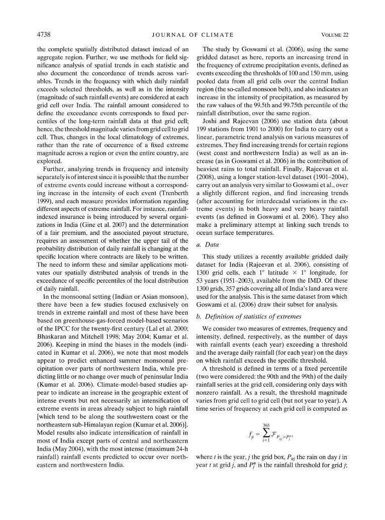
TABLE 1. Distribution of grids with statistically significant (at the αl = 10% significance level) trends (357 grid cells in total).

Number of grids with trend

Increasing Decreasing

90th percentile threshold Frequency 25 61 Intensity 44 27

99th percentile threshold Frequency 45 30 Intensity 42 25

direction of trends reported in Goswami et al. (2006) (with a fixed rainfall threshold) and in Joshi and Rajeevan (2006) (with a spatially varying threshold).

A perusal of the trends in frequency and intensity of exceedance of the 99th percentile threshold supports such a speculation, given the dominance of increasing trends in both frequency and intensity at this threshold. However, contrary to much of the literature, a fair number of decreasing trends are noted in our analyses. From the figures it is clear that, while the details vary by threshold and metric (frequency and intensity), increasing trends dominate in the coastal regions and in the eastern re­gion (west of Bangladesh), while decreasing trends ap­pear to be more prevalent in the northern, central, and northeastern parts of India. Indeed, from these figures, it is difficult to argue that there has been an increase in the frequency and intensity of extreme rainfall across India.

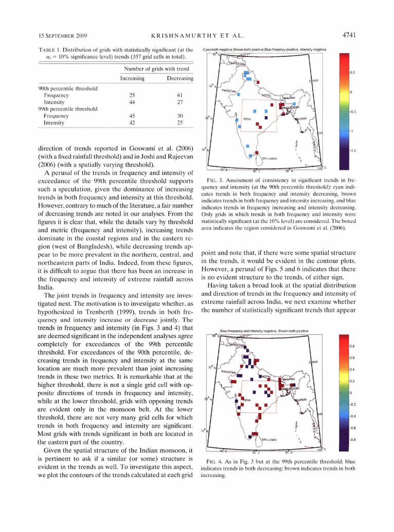
The joint trends in frequency and intensity are inves­tigated next. The motivation is to investigate whether, as hypothesized in Trenberth (1999), trends in both fre­quency and intensity increase or decrease jointly. The trends in frequency and intensity (in Figs. 3 and 4) that are deemed significant in the independent analyses agree completely for exceedances of the 99th percentile threshold. For exceedances of the 90th percentile, de­creasing trends in frequency and intensity at the same location are much more prevalent than joint increasing trends in these two metrics. It is remarkable that at the higher threshold, there is not a single grid cell with op­posite directions of trends in frequency and intensity, while at the lower threshold, grids with opposing trends are evident only in the monsoon belt. At the lower threshold, there are not very many grid cells for which trends in both frequency and intensity are significant. Most grids with trends significant in both are located in the eastern part of the country.

G i v e n the spatial structure of the Indian monsoon, it is pertinent to ask if a similar (or some) structure is evident in the trends as well . To investigate this aspect, we plot the contours of the trends calculated at each grid

FIG. 3. Assessment of consistency in significant trends in fre­quency and intensity (at the 90th percentile threshold): cyan indi­cates trends in both frequency and intensity decreasing, brown indicates trends in both frequency and intensity increasing, and blue indicates trends in frequency increasing and intensity decreasing. Only grids in which trends in both frequency and intensity were statistically significant (at the 10% level) are considered. The boxed area indicates the region considered in Goswami et al. (2006).

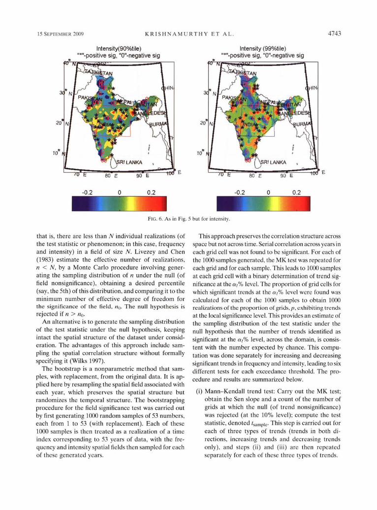
point and note that, if there were some spatial structure in the trends, it would be evident in the contour plots. However, a perusal of Figs. 5 and 6 indicates that there is no evident structure to the trends, of either sign.

Having taken a broad look at the spatial distribution and direction of trends in the frequency and intensity of extreme rainfall across India, we next examine whether the number of statistically significant trends that appear

FIG. 4. As in Fig. 3 but at the 99th percentile threshold: blue indicates trends in both decreasing: brown indicates trends in both increasing.

4742 JOURNAL OF CLIMATE VOLUME 22

FIG. 5. Contours of the trend estimated by the Sen slope for frequency of exceedance at each of the grids. Grids with statistically significant trends (at the 10% level of significance) are marked with an asterisk and 0. The boxed area indicates the region considered in Goswami et al. (2006).

to be different from zero at the 10% significance level could occur purely by chance, in an analysis of the spatially distributed dataset used here.

d. Field significance test

The question addressed in this section is whether the number of increasing or decreasing trends deemed significant at the gridcell level analysis could occur purely by chance, taking into account the possibility that the rainfall data, and hence the trends, have an underlying spatial structure. The answer to this ques­tion depends on the specific area or domain considered [all of India or the core monsoon region, as identified in Goswami et al . (2006) and indicated as a box in all figures]. Results for the all-India data are presented first and those for the smaller, core monsoon region are discussed next.

The so-called field significance test (Livezey and Chen 1983) has been typically used to address the question posed in this section. The nul l hypothesis of the test is that the number n out of N total grid cells exhibi t ing a trend at the αl% level of significance (local or at each grid cell) is not inconsistent wi th the value expected by chance, considering the potential for spatial correlat ion across the indiv idual time series analyzed for trends. The nul l hypothesis is rejected if n is larger than the number expected by chance

at the αf% significance level (global or across the domain) . 1

A one-sided test is used, to test whether the propor­tion of grids with significant trends p is greater than the (global) significance level αf, as below:

H0:p = αf vs Ha:p>αf.

The test statistic

is distributed N(0, 1) under the nul l .

In most applications, the validity of the field signifi­cance test is compromised by the finiteness of the dataset used and by the spatial and/or temporal correlation between the series used (Livezey and Chen 1983; Elmore et al. 2006; Wi lks 1997). W e outline a procedure that addresses the spatial dependence of data. Spatial correlation reduces the degree-of-freedom of the test;

1 Note that the local significance level αl is always taken to be 10%, while the global significance level αf is either 10% or 5% depending on whether the field significance test pertains to both increasing and decreasing (significant) trends or only increasing or decreasing trends.

15 SEPTEMBER 2009 KRISHNAMURTHY ET AL. 4743

FIG. 6. As in Fig. 5 but tor intensity.

that is, there are less than N individual realizations (of the test statistic or phenomenon; in this case, frequency and intensity) in a field of size N. Livezey and Chen (1983) estimate the effective number of realizations, n < N, by a Monte Car lo procedure involving gener­ating the sampling distribution of n under the null (of field nonsignificance), obtaining a desired percentile (say, the 5th) of this distribution, and comparing it to the minimum number of effective degree of freedom for the significance of the field, n0. The null hypothesis is rejected if n > n0.

An alternative is to generate the sampling distribution of the test statistic under the null hypothesis, keeping intact the spatial structure of the dataset under consid­eration. The advantages of this approach include sam­pling the spatial correlation structure without formally specifying it (Wilks 1997).

The bootstrap is a nonparametric method that sam­ples, with replacement, from the original data. It is ap­plied here by resampling the spatial field associated with each year, which preserves the spatial structure but randomizes the temporal structure. The bootstrapping procedure for the field significance test was carried out by first generating 1000 random samples of 53 numbers, each from 1 to 53 (with replacement). Each of these 1000 samples is then treated as a realization of a time index corresponding to 53 years of data, with the fre­quency and intensity spatial fields then sampled for each of these generated years.

This approach preserves the correlation structure across space but not across time. Serial correlation across years in each grid cell was not found to be significant. For each of the 1000 samples generated, the MK test was repeated for each grid and for each sample. This leads to 1000 samples at each grid cell with a binary determination of trend sig­nificance at the αl% level. The proportion of grid cells for which significant trends at the αl% level were found was calculated for each of the 1000 samples to obtain 1000 realizations of the proportion of grids, p, exhibiting trends

at the local significance level. This provides an estimate of the sampling distribution of the test statistic under the null hypothesis that the number of trends identified as significant at the αl% level, across the domain, is consis­tent with the number expected by chance. This compu­tation was done separately for increasing and decreasing significant trends in frequency and intensity, leading to six different tests for each exceedance threshold. The pro­cedure and results are summarized below.

(i) M a n n - K e n d a l l trend test: Carry out the MK test; obtain the Sen slope and a count of the number of grids at which the null (of trend nonsignificance) was rejected (at the 10% level); compute the test statistic, denoted tsample. This step is carried out for each of three types of trends (trends in both di­rections, increasing trends and decreasing trends only), and steps (ii) and (iii) are then repeated separately for each of these three types of trends.

4744 JOURNAL OF CLIMATE VOLUME 22

TABLE 2. Bootstrap test results [note i) t: raw statistic; t*: critical value—the (1 - αf) quantile of the bootstrap distribution ii) αf for increasing and decreasing trends is 0.05, while for all significant grids it is 0.1 and iii) null of field nonsignificance (p = αf) is rejected if t > t*].

Trend

Frequency Intensity

Trend t* t Null t* t Null

90th percentile threshold Both increasing and decreasing -0.078 0.141 Reject -0.042 0.099 Reject Increasing only 0.025 -0.03 Do not -0.039 0.023 Reject Decreasing only -0.073 0.071 Reject 0.008 -0.024 Do not

99th percentile threshold Both increasing and decreasing -0.056 0.11 Reject -0.034 0.088 Reject Increasing only -0.039 0.026 Reject -0.031 0.018 Reject Decreasing only 0 -0.016 Do not 0.014 -0.03 Do not

(ii) F i e ld significance test: • Randomly sample, with replacement from the

data, to obtain 1000 copies of the data matrix while retaining the spatial structure.

• Obta in 1000 realizations of the proportion of the grid cells, p, for which the hypothesis of no trend is rejected and the vector (of size 1000) of test

statistics (denoted tbootstrap). • Construct the bootstrap estimate of the sampling

distribution of the test statistic Tbootstrap = (tbootstrap - tsample). Sort this vector and obtain its

100(1 - αf)th percentile (denoted T*).2

• Test T = tsample - αf against T* (recall that a one-sided test is employed) 3 and reject the null hypothesis that the number of significant trends is what would be expected by chance i f T > T*.

(iii) Repeat the analysis for different thresholds.

The results of the bootstrap procedure are summa­rized in Table 2. First , if we consider the total number of trends (of either sign), we observe that the null hy­pothesis is rejected for all tests. Next , if we consider increasing trends only in the case of frequency of ex­ceedance of the 90th percentile is the null hypothesis not rejected. Changes in intensity indicate an increasing trend at both thresholds. The number of decreasing trends passes the significance test only for frequency at the 90th percentile. Thus, in summary, the hypothesis that overall there is an increasing trend in the frequency and intensity of extreme rainfall appears to have sup­port with the caveat that, at the 90th percentile, the frequency of exceedance appears to be decreasing in the central and northern regions, while the intensity

of these events is increasing. A contour plot of the slopes of frequency and intensity provides a smoother representation of the nature of these trends (Figs. 5 and 6).

Now consider the results over the region considered by Goswami et al. (2006), the main study with a similar analysis and dataset. Recal l that Goswami et al. define extremes over a homogeneous region and use the number of days of rainfall above 100 and 150 mm and the intensity of rainfall for a fixed percentile (99.5th and 99.75th) as measures of extremes. They report an increase in the frequency of extreme rainfall events as well as an increase in the intensity of extreme rainfall. Carrying out the field significance test outlined in the preceding section over their domain, we find that the broad conclusions from the national analysis are essentially unchanged (Tables 3 and 4); that is, while increasing trends do exist, they are more predominant in the southwestern coast and north­eastern regions, with decreasing trends being more promi­nent in the central regions.

Joshi and Rajeevan (2006), using a different dataset, find increasing trends (using somewhat different measures of extremes) in very similar regions; they also report negative trends (at only two stations).

Goswami et al. (2006) also performed a split sample analysis, splitting the data into two parts, pre- and post­-1981, and find an increasing trend in the post-1981

TABLE 3. Distribution of grids with statistically significant (at αl = 10% significance level) trends in the region defined by

Goswami et al. (2006) (74 grid cells in total).

Number of grids with slopes

Increasing Decreasing

90th percentile threshold Frequency 7 9 Intensity 17 2

99th percentile threshold Frequency 13 4 Intensity 12 4

2 This is known as the "percentile method" of bootstrap-based hypothesis testing (Davison and Hinkley 1997, 201-203).

3 We note that this approach differs from the conventional one, involving testing Tbootstrap vs α; the approach adopted here is more efficient than the conventional one (Hall and Wilson 1991; Wilks 1997).

15 SEPTEMBER 2009 KRISHNAMURTHY ET AL. 4745

TABLE 4. Bootstrap test results for slopes in region defined by Goswami et al. (2006) [note i) t: raw statistic; t*: critical value—the (1 - αf) quantile of the bootstrap distribution ii) αf for increasing and decreasing trends is 0.05, while for all significant grids, it is 0.1 and iii) null of field nonsignificance (p = αf) is rejected if t > t*].

Trend

Frequency Intensity

Trend t* t Null t* t Null

90th percentile threshold Both increasing and decreasing -0.014 0.103 Reject -0.068 0.143 Reject Increasing only 0.041 -0.019 Do not -0.122 0.116 Reject Decreasing only 0 0.022 Reject 0.068 -0.073 Do not

99th percentile threshold Both increasing and decreasing -0.041 0.116 Reject -0.027 0.103 Reject Increasing only -0.054 0.062 Reject -0.054 0.049 Reject Decreasing only 0.041 -0.046 Do not 0.041 -0.046 Do not

sample. We repeated our analysis for the same two subperiods. The results of this analysis indicate that the conclusions obtained using the full sample are unaltered, unlike Goswami et al. who find a increasing trend only in the post-1981 sample. The importance of the spatially distributed analysis performed here is that, if the spatial differences noted represent nonhomogeneous aspects of the monsoon, then the spatial patterns identified in the trends would potentially help inform mechanism iden­tification and model performance evaluation.

K u m a r et al. (2006) find significant increases in in­tense precipitation in much of western, northwestern, and especially the southwestern regions. The results of the present analysis indicate trends mostly in parts of the southwestern coastal regions, similar to the results of K u m a r et al., as well as in the eastern and central regions. M a y (2004) reports increases over much of the Indian peninsula, while the coarse spatial resolution of the model used does not provide detail over smaller regions of India. Further, our results that decreasing trends are likely in many areas are in concurrence with M a y (2004), who also finds similar decreases (in the scale and/or shape parameters of the gamma or the Generalised Pareto (GPA) distributions, which are fit to the rainfall data) for a small number of regions. H o w ­ever, the spatial coarseness of the model prevents a closer spatial comparison of the results.

2. Discussion and conclusions

An earlier examination of trends in extremes of In­dian monsoon rainfall was developed further in this work. The analysis considered the spatial structure of changes in the extremes across the country rather than over a box (homogenous region) in central India. Broadly speaking, there is support for the hypothesis that the frequency and intensity of extreme rainfall over India may be increasing over the previous 53 years.

However, there is considerable spatial variation as to the direction of change, and the spatial continuity of trends deemed statistically significant is weak. This is not unexpected since threshold crossings are a random process and the assessment of significance is also a threshold process. A visual examination of the spatial variation in the trends in frequency and intensity of extreme rainfall suggests that the north and central sections of the Indian Subcontinent have experienced a generally decreasing trend in the frequency and inten­sity of extremes, while the coastal regions in peninsular India and the region immediately west of Bangladesh have experienced increasing trends.

Even in central India, which was analyzed in aggre­gate by a previous study, there is some heterogeneity in the direction of the trends, and the larger-scale analysis performed here helps clarify the spatial structure of the changes in the region studied in Goswami et al. (2006).

W e do not attribute the trends observed to anthro­pogenic climate change or to interdecadal climate vari­ability, which may be of natural origin. Rather, we offer the results of this analysis as a benchmark to the climate community to consider more detailed studies of the spatial structure of changes in the Indian monsoon mechanisms so that a better informed attribution of change can be determined.

General ly, it is known that tropical depressions that form in the Bay of Bengal and then propagate westward or northward play a key role in extreme rainfall. These are associated with a mix of barotropic and baroclinic instabilities and their interaction with the mean mon­soonal flow (Gadgi l 2003). W e suspect that the details of these interactions may be associated with the indicated changes in the spatial structure of the trends and, nat­urally, with the trends themselves. A recent study by Guhathakurta and Rajeevan (2008) notes a significant decreasing trend in the frequency of depressions and storms over the Bay of Bengal, lending support to our

4746 JOURNAL OF CLIMATE VOLUME 22

conjecture. Model-based studies and detailed analysis

of individual extreme events are necessary to develop

this intuition and are being pursued.

The design of our study was somewhat different from

prior work. First, we considered changes in the cl ima­

tology of extremes for each spatial location, rather than

the frequency and intensity of exceedance of a fixed

threshold, which is more meaningful for an analysis of

the larger spatial scale considered. Second, instead of

considering linear trends, we considered the more gen­

eral case of monotonic trends (this would include, e.g., a

step change in the process at some time or an expo­

nential or logarithmic trend) and assessed the evidence

for such a trend using robust, nonparametric methods.

The field significance test was applied both nationally

and regionally and essentially confirms that the number

of cases for which the null hypothesis of no trend was

rejected was statistically different from that obtained

purely by chance (at the relevant level of significance).

Thus, our study lends credibility to previous assess­

ments that report increasing trends in frequency and

intensity of extreme rainfall over India, while identify­

ing areas where there is a systematic departure from

previous assessments. The issue of how these trends

may be reinforced or reversed over the twenty-first

century is not addressed here and is the subject of on­

going investigation. However, we note that the broad

direction of trends identified here is consistent with the

expectation from the model-based analysis for the twenty-

first century scenarios for climate change, as reported by

Kumar et al. (2006) and M a y (2004).

Acknowledgments. W e wish to acknowledge the as­

sistance of Dr M. Rajeevan, Director (NCC), Indian

Meteorological Department, Pune, whose support was

instrumental in obtaining the dataset on which the

present analyses is based. W e are also grateful to two

anonymous reviewers for providing suggestions that

helped improve the quality of the paper.

REFERENCES

Alexander, L. V., and Coauthors, 2006: Global observed changes in daily climate extremes of temperature and precipitation. J. Geophys. Res., 111, D05109, doi:10.1029/2005JD006290.

Bhaskaran, B., and J. Mitchell, 1998: Simulated changes in southeast Asian monsoon precipitation resulting from an­thropogenic emissions. Int. J. Climatol., 15, 1455-1462.

Davison, A. C., and D. V. Hinkley, 1997: Bootstrap Methods and Their Application. Cambridge Series in Statistical and Probabilistic Mathematics, No. 1, Cambridge University Press, 582 pp.

Elmore, K. L., M. E. Baldwin, and D. M. Schultz, 2006: Field significance revisited: Spatial bias errors in forecasts as ap­plied to the eta model. Mon. Wea. Rev., 134, 519-531.

Gadgil, S., 2003: The Indian monsoon and its variability. Annu. Rev. Earth Planet. Sci., 31, 429-467.

Gine, X., R. Townsend, and J. Vickrey, 2007: Statistical analysis of rainfall insurance payouts in southern India. Amer. J. Agric. Econ., 89, 1248-1254.

Goswami, B., V. Venugopal, D. Sengupta, M. Madhusoodanan. and P. K. Xavier, 2006: Increasing trends of extreme rain events over India in a warming environment. Science, 314, 1442-1444.

Guhathakurta, P., and M. Rajeevan, 2008: Trends in the rainfall pattern over India. Int. J. Climatol, 28, 1453-1469.

Hall, P., and S. Wilson, 1991: Two guidelines for bootstrap hy­pothesis testing. Biometrics, 47, 757-762.

Helsel, D. R., and R. M. Hirsch, 1992: Statistical Methods in Water Resources. Studies in Environmental Science, Vol. 49, Elsevier Science, 522 pp.

Joshi, U., and M. Rajeevan, 2006: Trends in precipitation extremes over India. Tech. Rep. 3, National Climate Centre, 25 pp.

Klein Tank, A. M. G., and Coauthors, 2006: Changes in daily tem­perature and precipitation extremes in central and south Asia. J. Geophys. Res., 111, D16105, doi:10.1029/2005JD006316.

Kumar, K. R., A. K. Sahai, K. K. Kumar, S. K. Patwardhan, P. K. Mishra, J. V. Revadekar, K. Kamala, and G. B. Pant, 2006: High-resolution climate change scenarios for India for the 21st century. Curr. Sci., 90, 332-345.

Lal, M., G. A. Meehl, and J. M. Arblaster, 2000: Simulation of Indian summer monsoon rainfall and its intraseasonal vari­ability. Reg. Environ. Change, 1, 163-179.

Livezey, R. E., and W. Chen. 1983: Statistical field significance and its determination by Monte Carlo techniques. Mon. Wea. Rev., 111, 46-59.

May, W., 2004: Simulation of the variability and extremes of daily rainfall during the Indian summer monsoon and future times in a global time-slice experiment. Climate Dyn., 22,183-204.

Rajeevan, M., J. Bhate, J. Kale, and B. Lal, 2006: High resolution daily gridded rainfall data for the Indian region: Analysis of break and active monsoon spells. Curr. Sci., 91, 296-306. —, —, and A. Jaswal, 2008: Analysis of variability and trends of extreme rainfall events over India using 104 years of gridded daily rainfall data. Geophys. Res. Lett., 35, L18707, doi:10.1029/2008GL035143.

Trenberth, K., 1999: Conceptual framework for changes of ex­tremes of the hydrological cycle with climate change. Climatic Change, 42, 327-339.

Wilks, D., 1997: Resampling hypothesis tests for autocorrelated fields. J. Climate, 10, 65-82.

Yue, S., P. Pilon, and G. Cavadias, 2002: Power of the Mann­-Kendall and Spearman's rho tests for detecting monotonic trends in hydrological series. J. Hydrol., 259, 254-271.

COPYRIGHT INFORMATION

TITLE: Changing Frequency and Intensity of Rainfall Extremesover India from 1951 to 2003

SOURCE: J Clim 22 no18 S 15 2009

The magazine publisher is the copyright holder of this article and itis reproduced with permission. Further reproduction of this article inviolation of the copyright is prohibited.