Ocean Modelling 15 (2006) 141–156

www.elsevier.com/locate/ocemod

Changes in ocean ventilation during the 21st Centuryin the CCSM3 q

Frank O. Bryan *, Gokhan Danabasoglu, Peter R. Gent, Keith Lindsay

National Center for Atmospheric Research, P.O. Box 3000, Boulder, CO 80307-3000, USA

Received 9 July 2005; received in revised form 28 December 2005; accepted 5 January 2006Available online 23 February 2006

Abstract

Changes in the ventilation rate of the global ocean during the 20th and 21st centuries, as indicated by changes in thedistribution of ideal age, are examined in a series of integrations of the Community Climate System Model version 3. Theglobal mean age changes little in the 20th Century relative to pre-industrial conditions, but increases in the 21st Century,by an amount that is independent of the range of climate forcings considered. The increase is primarily due to a decrease inthe ventilation rate of Antarctic Bottom Water (AABW), and to a lesser degree, North Atlantic Deep Water (NADW).Changes in a regional volumetric census of age indicate that the changes in AABW are predominantly for waters thatare already older than 100 years, so will likely have a moderate direct feedback on oceanic uptake of CO2 and other tracers.On the other hand, the changes in NADW occur most strongly in waters that are a few decades old, so are more likely tohave a feedback on the climate system. While the global mean age increases, the age does not increase everywhere in theocean. Regions newly exposed to strong atmospheric forcing as sea ice retreats experience an increase in convection anddecreasing age. Age also decreases over a large volume of the lower thermocline as the rate of upwelling of old deep waterdecreases with the weakening of the thermohaline circulation.� 2006 Elsevier Ltd. All rights reserved.

Keywords: Ocean ventilation; Water mass age

1. Introduction

Studies of the ocean response to climate change forcing have largely focused on the issues of ocean heatuptake (e.g. Gent et al., in press), sea level rise (e.g. Church and Gregory, 2001), the stability of the thermo-haline circulation (e.g. Wood et al., 2003), and changes in water mass properties (e.g. Banks et al., 2002). Eachof these issues can be related to the process of ocean ventilation, i.e., the rate and pathways by which surfacewaters are carried into the interior of the ocean (e.g. Church et al., 1991). Understanding the response ofventilation processes will become even more important as we begin to try to understand feedbacks between

1463-5003/$ - see front matter � 2006 Elsevier Ltd. All rights reserved.

doi:10.1016/j.ocemod.2006.01.002

q Submitted to the special issue of Ocean Modelling: Oceanic results from a new generation of coupled climate models.* Corresponding author. Tel.: +1 303 497 1394; fax: +1 303 497 1700.

E-mail address: bryan@ucar.edu (F.O. Bryan).

142 F.O. Bryan et al. / Ocean Modelling 15 (2006) 141–156

climate change and the rate of uptake of anthropogenic CO2 by the ocean (Fung et al., 2005). Yet, there havebeen relatively few studies that directly address changes in ocean ventilation in the late 20th Century (Doneyet al., 1998; Watanabe et al., 2001) or that make projections of ocean ventilation rates under climate changeforcing in the coming century. In this study, we present an initial analysis along these lines, evaluating changesin ocean ventilation in response to a range of climate change scenarios as simulated by the CommunityClimate System Model version 3 (CCSM3).

One measure of ocean ventilation is the distribution of age, defined as the time since a water parcel was lastat the sea surface. Observational estimates of water mass age have been derived from measurements of a vari-ety of tracers including natural and bomb radioisotopes and CFCs. Observational programs such as CLIVAR(www.clivar.org/carbon_uptake) are now underway to make systematic repeat global surveys of these tracersin order to detect variability in ocean ventilation rates and carbon storage. The ability of ocean models toreproduce the distributions of these tracers, and the age measures derived from them, provides a strong testof the reliability of their simulation of ventilation processes (England and Maier-Reimer, 2001; Gent et al., inpress). However, these tracer based age measures are subject to biases relative to the true mean water mass ageas a result of mixing and the nonlinearity of their input time histories (Waugh et al., 2003). Thiele and Sar-miento (1990) proposed a tracer for use in simulation studies, called ideal age, that provides an unbiased esti-mate of ventilation time scales. Ideal age has a surface boundary condition of zero concentration, and aninterior source strength of one unit per year. It is advected and diffused in the same manner as temperatureor salinity, and thus acts as a clock accumulating time since last contact with the sea surface. Further, underconditions of statistically stationary flow, ideal age can be shown to be equal to the first moment of the prob-ability distribution of transit times from the sea surface, which itself is a complete characterization of thetransport capacity of the flow (Waugh et al., 2003).

Ideal age was included in all CCSM3 integrations carried out for the IPCC Fourth Assessment Report inorder to provide a diagnostic for examining changes in ocean ventilation in response to climate forcing. Bryanet al. (in press) examined changes in ideal age in the North Atlantic Ocean between CCSM3 present daycontrol runs and 1% per year increasing CO2 experiments in the context of an analysis of the response ofthe meridional overturning circulation and its dependence on component model resolution. Bitz et al. (inpress) analyze changes in ideal age in the Arctic Ocean from the same 1% per year increasing CO2 experiment,as a measure of changes in convective activity that accompany increases in the fraction of open water as theclimate warms. In this paper, we analyse changes in the distribution of ideal age in the CCSM3 20th Centuryhistorical and several 21st Century scenario ensembles. In contrast to the papers cited above, the focus here isprimarily on ventilation, and the perspective is more global. We address the questions: Do ocean ventilationrates increase or decrease? Where are the largest changes? What range of initial ages are most stronglyimpacted? What water masses are affected? How does the response of the age distribution depend on thestrength of the climate forcing scenarios?

2. The CCSM3 ocean component and experiments

The ocean component of the CCSM3 is based on the POP code developed at Los Alamos National Lab-oratory. It uses a dipole grid (Smith et al., 1995) with the grid north pole singularity displaced into Greenlandat 80� N, 40� W. The horizontal grid has 320 (zonal) · 384 (meridional) grid points, and the resolution is uni-form in the zonal, but not in the meridional, direction. The meridional grid spacing varies from a minimum of0.27� at the equator, gradually increasing to a maximum of 0.66� at mid-latitudes. There are 40 levels in thevertical, whose thickness increases from 10 m near the surface to 250 m in the deep ocean. The minimum andmaximum depths are 30 m and 5.5 km. The domain is global, with open connections to Hudson Bay, the Med-iterranean Sea, and the Persian Gulf and an open Bering Strait. The time step used is 1 h, which is smallenough that no Fourier filtering is required around the displaced Greenland pole.

The horizontal viscosity is an anisotropic Laplacian operator in the form suggested by Smith and McWil-liams (2003), which uses different coefficients in the east–west and north–south directions. The vertical mixingscheme is the K-profile parameterization (KPP) scheme of Large et al. (1994), and the mesoscale eddy param-eterization is that of Gent and McWilliams (1990). A third-order upwind advection scheme is used, see Hol-land et al. (1998). This scheme is not monotonic and can give mild overshoots and undershoots in ideal age.

Table 1Numerical experiments used in this study are indicated by an X

Member Initial condition 20C TCC B1 A1B A2

1 C1 – 360 X X X2 C1 – 380 X X X X X3 C1 – 400 X X4 C1 – 420 X X5 C1 – 440 X X6 C2 – 380 X X X7 C2 – 410 X X X8 C2 – 460 X X X9 C2 – 540 X

C1 and C2 refer to the two pre-industrial controls, and the year refers to the date of the control that the initial condition for that ensemblemember family was taken. All dates refer to the start of the year shown.

F.O. Bryan et al. / Ocean Modelling 15 (2006) 141–156 143

Further details of the CCSM3 ocean component can be found in Danabasoglu et al. (in press) and Smith andGent (2004).

The atmospheric component model used in the experiments described here, CAM3, has T85 spectral trun-cation, or approximately 1.4� grid spacing. The land component model, CLM3, runs on the same grid as theatmospheric model, but includes a sub-grid scale representation of surface type heterogeneity. The sea icecomponent, CSIM4, runs on the same grid as the ocean model and includes a sub-grid scale representationof ice thickness categories. The component models are coupled through a flux coupler, and the ocean commu-nicates with the other components once per simulated day. As a point of reference, this configuration of theCCSM3 model has an equilibrium climate sensitivity to doubling of CO2 of 2.7 �C, and a transient climateresponse to 1% compound increase of CO2 of 1.5 �C at the time of doubling. Further details on the modelsand the characteristics of their coupled and uncoupled control simulations can be found in Collins et al.(in press) and references therein.

A pre-industrial control integration of the coupled system, from which all other CCSM3 IPCC experimentswere branched, was initialized with the ocean at rest and with modern day potential temperature and salinity,but pre-industrial concentrations of greenhouse gases and aerosols and run for 510 years. A second pre-indus-trial control ensemble member was branched from this simulation at year 300 (this branch and those listedbelow occur on 1 January of the year indicated) and run through year 950. A list of all the historical and futurescenario experiments used in this analysis is shown in Table 1. The initial states for the 20th Century historicalforcing experiments (20C hereafter) were taken from the two pre-industrial controls between years 360 and540 as indicated in Table 1 and run for the period 1870–2000. In the 20C experiments greenhouse gas concen-trations, aerosol emissions (including volcanic), and solar variability were prescribed from historical data.From the end of each 20C experiment a set of scenarios for the 21st Century were carried out. In the first sce-nario, referred to as 20th Century commitment (TCC hereafter), greenhouse gas concentrations and aerosolemissions were held fixed at their year 2000 levels. Climate change experiments following the IPCC SpecialReport Emissions Scenarios (SRES) B1, A1B and A2 were also run from the end of the 20C integrations.These represent low, medium, and high greenhouse gas emission scenarios, respectively. The global ensemblemean surface air temperature response at the end of the 21st Century relative to the end of the 20th Century is0.6 �C for the TCC scenario, and 1.5 �C, 2.6 �C, and 3.5 �C for the Bl, A1B, and A2 scenarios, respectively(Meehl et al., 2005). A total of nine ensemble members were run for the historical integrations, but not everyensemble member was run for every 21st Century scenario and some results were not available to us for thisstudy because of data management issues.

3. Spin-up and equilibration of ideal age

The ideal age tracer in our experiments was initialized to zero at the start of the first pre-industrial controlintegration. It was not reset when subsequent integrations, either the second pre-industrial control, or the 20thand 21st Century integrations, were branched. Fig. 1 shows the evolution of the horizontal mean age over the

Fig. 1. Timeseries of horizontal mean ideal age (years) versus depth over the Pacific Ocean from the pre-industrial control experiment.

144 F.O. Bryan et al. / Ocean Modelling 15 (2006) 141–156

Pacific Ocean through the period of the pre-industrial control experiment. The 20th and 21st Century exper-iments used in this analysis overlap the control between years 360 and 770. During this period, the horizontalmean ideal age is equilibrated only in the upper few hundred meters. The oldest waters are found at 2.4 kmand are just beginning to show signs of the influence of surface waters at the end of this period by growing atless than one unit per year. At the end of the 950 year integration, the maximum horizontal mean age is 675–700 years. In a very long integration of a coarser resolution, but similarly configured version of the POP oceanmodel, Peacock and Maltrud (in press) have shown that it takes in excess of 4000 years for the global mean ageto converge, and the oldest waters in the mid-depth North Pacific have ages of 1600–1700 years. A similarmaximum ideal age of 1500 years was found in a global ocean simulation by England (1995).

The incomplete spin-up of age introduces a degree of uncertainty in the results and limits comparisons withobserved tracer ages for older water masses. However, we are motivated to proceed with the analysis for tworeasons. First, there is relatively little information on projected changes in ventilation, so we should try tomake the best use of the results that are available. We can at least learn something about the sign of trendsand locations of changes by looking at differences in the scenario experiments relative to the drifting controlsimulation. In the following, when we perform differences between epochs we correct for age drift by subtract-ing the change in age of the pre-industrial control experiment over the same time interval as the experiments inquestion, i.e.,

dAðt2; t1Þ ¼ ðAE2ðt2Þ � AE1ðt1ÞÞ � ðACðt2Þ � ACðt1ÞÞ ð1Þ

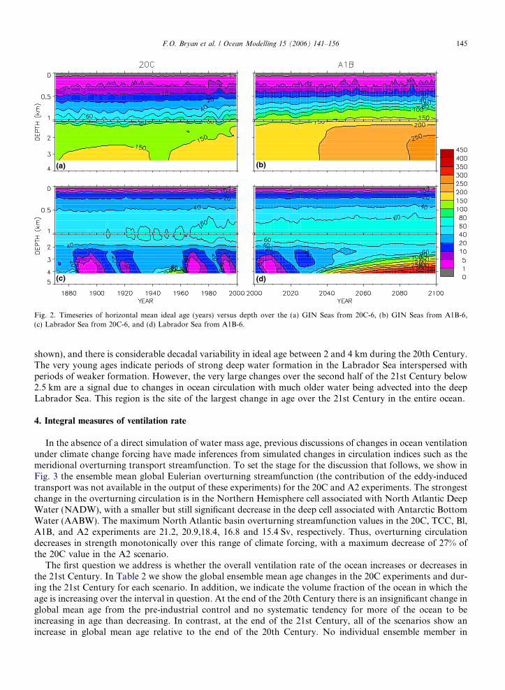
where AE1, AE2, AC denote the age field of experiments E1, E2, and the control respectively, and t1 and t2 de-note the time of the epochs being differenced. Unless otherwise noted, when we refer to age changes we arereferring to changes adjusted for drift as defined above. Also, the epochs between which we consider differ-ences are 20 year time averages from the beginning and end of the 20th Century integrations, i.e., 1870–1890 and 1980–2000, and the end of the 21st Century scenario experiments, 2080–2100.

Second, in considering the response to climate change forcing over the next century we are particularlyinterested in those waters with relatively young ages. Those will have been directly exposed to the transientclimate forcing and therefore play a role in carrying the climate change signal into the interior of the oceanand in the sequestration of anthropogenic CO2. These younger waters are closer to being equilibrated thanthe very old waters. In regions where deep water formation or strong subduction are occurring, ages are youngand have equilibrated through more of the water column than just the surface layers. For example, Fig. 2a andb shows age horizontally averaged over the Greenland, Iceland, and Norwegian (GIN) Seas as a function ofdepth for ensemble member 20C-6 from 1870 to 2000 and ensemble member A1B-6 from 2000 to 2100. Agehas equilibrated down to at least 1.5 km by year 380 of the control run in this basin (not shown), so that thechanges in age shown in the figure at 0.8–1.2 km depth between 1980 and 2050 are a signal due to the changesin ocean circulation during that time, and are not model drift. Fig. 2c and d also shows age versus depth, butfor the Labrador Sea. In this basin, age has equilibrated at all depths by year 380 of the control run (not

(a) (b)

(c) (d)

Fig. 2. Timeseries of horizontal mean ideal age (years) versus depth over the (a) GIN Seas from 20C-6, (b) GIN Seas from A1B-6,(c) Labrador Sea from 20C-6, and (d) Labrador Sea from A1B-6.

F.O. Bryan et al. / Ocean Modelling 15 (2006) 141–156 145

shown), and there is considerable decadal variability in ideal age between 2 and 4 km during the 20th Century.The very young ages indicate periods of strong deep water formation in the Labrador Sea interspersed withperiods of weaker formation. However, the very large changes over the second half of the 21st Century below2.5 km are a signal due to changes in ocean circulation with much older water being advected into the deepLabrador Sea. This region is the site of the largest change in age over the 21st Century in the entire ocean.

4. Integral measures of ventilation rate

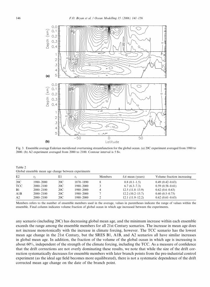
In the absence of a direct simulation of water mass age, previous discussions of changes in ocean ventilationunder climate change forcing have made inferences from simulated changes in circulation indices such as themeridional overturning transport streamfunction. To set the stage for the discussion that follows, we show inFig. 3 the ensemble mean global Eulerian overturning streamfunction (the contribution of the eddy-inducedtransport was not available in the output of these experiments) for the 20C and A2 experiments. The strongestchange in the overturning circulation is in the Northern Hemisphere cell associated with North Atlantic DeepWater (NADW), with a smaller but still significant decrease in the deep cell associated with Antarctic BottomWater (AABW). The maximum North Atlantic basin overturning streamfunction values in the 20C, TCC, Bl,A1B, and A2 experiments are 21.2, 20.9,18.4, 16.8 and 15.4 Sv, respectively. Thus, overturning circulationdecreases in strength monotonically over this range of climate forcing, with a maximum decrease of 27% ofthe 20C value in the A2 scenario.

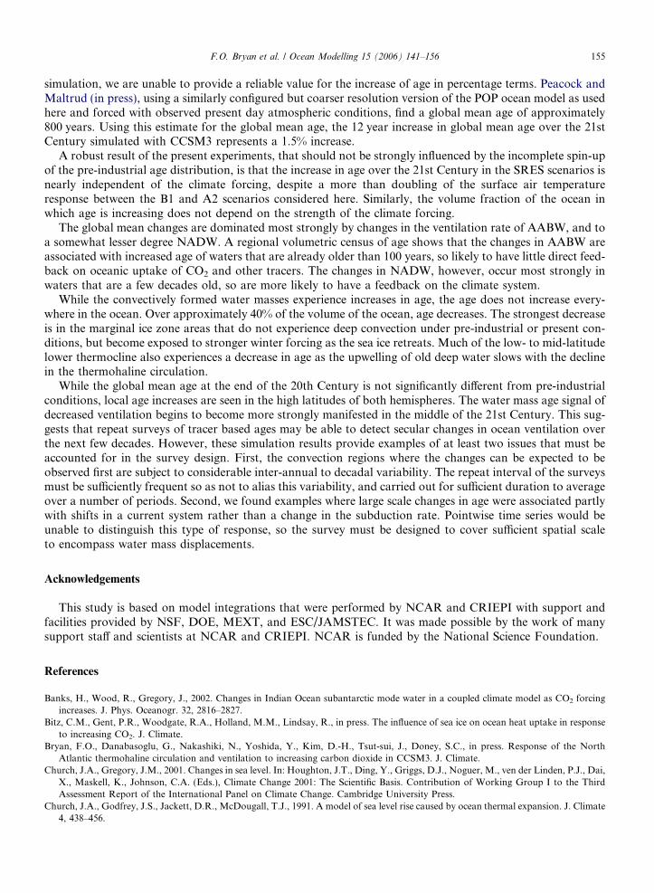
The first question we address is whether the overall ventilation rate of the ocean increases or decreases inthe 21st Century. In Table 2 we show the global ensemble mean age changes in the 20C experiments and dur-ing the 21st Century for each scenario. In addition, we indicate the volume fraction of the ocean in which theage is increasing over the interval in question. At the end of the 20th Century there is an insignificant change inglobal mean age from the pre-industrial control and no systematic tendency for more of the ocean to beincreasing in age than decreasing. In contrast, at the end of the 21st Century, all of the scenarios show anincrease in global mean age relative to the end of the 20th Century. No individual ensemble member in

(a)

(b)

Fig. 3. Ensemble average Eulerian meridional overturning streamfunction for the global ocean. (a) 20C experiment averaged from 1980 to2000. (b) A2 experiment averaged from 2080 to 2100. Contour interval is 5 Sv.

Table 2Global ensemble mean age change between experiments

E2 t2 E1 t1 Members dA mean (years) Volume fraction increasing

20C 1980–2000 20C 1870–1890 8 0.8 (0.1–1.5) 0.49 (0.42–0.63)TCC 2080–2100 20C 1980–2000 3 6.7 (6.3–7.3) 0.59 (0.58–0.61)B1 2080–2100 20C 1980–2000 4 12.5 (11.8–13.9) 0.62 (0.6–0.63)A1B 2080–2100 20C 1980–2000 7 12.2 (10.2–15.7) 0.60 (0.5–0.73)A2 2080–2100 20C 1980–2000 2 12.1 (11.9–12.2) 0.62 (0.61–0.63)

Members refers to the number of ensemble members used in the average, values in parentheses indicate the range of values within theensemble. Final column indicates volume fraction of global ocean in which age increased between the experiments.

146 F.O. Bryan et al. / Ocean Modelling 15 (2006) 141–156

any scenario (including 20C) has decreasing global mean age, and the minimum increase within each ensembleexceeds the range among the ensemble members for all 21st Century scenarios. The increase in mean age doesnot increase monotonically with the increase in climate forcing, however. The TCC scenario has the lowestmean age change in the 21st Century, but the SRES B1, A1B, and A2 scenarios all have similar increasesin global mean age. In addition, the fraction of the volume of the global ocean in which age is increasing isabout 60%, independent of the strength of the climate forcing, including the TCC. As a measure of confidencethat the drift corrections are not overly dominating these results, we note that while the size of the drift cor-rection systematically decreases for ensemble members with later branch points from the pre-industrial controlexperiment (as the ideal age field becomes more equilibrated), there is not a systematic dependence of the driftcorrected mean age change on the date of the branch point.

F.O. Bryan et al. / Ocean Modelling 15 (2006) 141–156 147

As indicated above, the degree to which age changes will have a direct feedback on climate change and car-bon sequestration depends on the initial age of the waters that are affected. To address this question, we per-form a volume census of age, i.e., compute the volume of water within a sequence of ranges of age (taken hereas 2 year intervals), and examine the changes in the census in response to climate forcing. Fig. 4 shows thepercentage changes in the volume of water with a given age for each scenario, integrated over the SouthernHemisphere Ocean. The largest signal is the 40–80% decrease in the volume of water with age in the rangeof 175–300 years and increase in the volume of waters with ages greater than 300 years (Fig. 4b–e). As willbe discussed further below, this represents a decrease in the ventilation rate of AABW under climate forcing.This signal even emerges weakly at the end of the 20th Century (Fig. 4a), primarily at the lower end of thisrange of ages. As in the case of the global mean age (Table 2), there is not a substantial difference in theresponse of AABW between the B1, A1B, and A2 scenarios.

Considering more recently ventilated waters, we see a weaker decrease in the volume of water with agesbetween 10 and 20 years, with increases in the volume of adjacent younger and older categories. While weakerin both percentage and absolute terms than the AABW change, the pattern seems robust across the scenarios.In contrast to the response of AABW, the volume shifts in the younger waters do become larger as the climateforcing increases. When considering individual sectors of the Southern Hemisphere Oceans, the shift in

(a)

(b) (c)

(d) (e)

Fig. 4. Percentage change in the volume of water with a given age integrated over the Southern Hemisphere oceans. Ensemble mean isshown as thick line, minimum and maximum changes among the ensemble members as thin lines: (a) difference between 20 year mean1870–1890 and 1980–2000 in 20C, (b) TCC vs. 20C, (c) B1 vs. 20C, (d) A1B vs. 20C, and (e) A2 vs. 20C.

148 F.O. Bryan et al. / Ocean Modelling 15 (2006) 141–156

ventilation rate of the bottom water is manifested most strongly in the South Atlantic and South IndianOceans, and is apparent but somewhat weaker in amplitude in the South Pacific. For the changes of volumein the age range of 10–30 years, the changes are again strongest in the South Indian Ocean, and clear in theSouth Pacific, but not reflected in the South Atlantic.

In the North Pacific (Fig. 5), changes in volume for ages greater than 100 years are very noisy with no dis-cernable systematic pattern across the scenarios. There is a general tendency for decreasing volumes of waterwith ages under 100 years, with the strongest decreases centered around 40 and 80 years reaching 20–30% inthe 21st Century. The spread among the ensemble members, especially at lower ages, is larger in the NorthAtlantic (Fig. 6) than for the other basins, probably reflecting the strong decadal timescale natural variabilitymentioned above. In the North Atlantic the strongest signal to emerge is the decrease in volume of water withage near 20 years for the B1, A1B, and A2 scenarios. This is the signature of decreased ventilation of NADW.

Thus, we see changes in the ventilation rates across a spectrum of ages including younger waters that weexpect to be directly exposed to anthropogenic tracers and climate change forcing. The strongest responseto climate forcing in the volume census of age is, however, a shift to older ages of already moderately oldAABW.

(a)

(b) (c)

(d) (e)

Fig. 5. As in Fig. 4 except for North Pacific Ocean.

(a)

(b) (c)

(d) (e)

Fig. 6. As in Fig. 4 except for North Atlantic Ocean.

F.O. Bryan et al. / Ocean Modelling 15 (2006) 141–156 149

5. Spatial distribution of ideal age changes over the 21st Century

Fig. 7a shows the ensemble mean, zonally averaged ideal age in the Atlantic Ocean averaged between 1980and 2000 from 20C, and the ensemble mean change in age at the end of the 20th Century relative to pre-indus-trial conditions. For present day conditions, water with ages less than 40 years reach down below 2 kmbetween 45� and 65� N, in contrast to about 125 m in the equatorial region. Ideal age is greater than 300 yearsat 1 km depth between 30� S and 5� N. The oldest waters, with age greater than 450 years, are found at 4.5 kmdepth between 45� and 50� N. Near Antarctica, water with ages less than 10 years reaches down to the depthof the Weddell Sea shelf, but in the zonal mean, water with age less than 100 years does not appear offshore ofthe continental slope. A local minimum in age of 175 years occurs at the base of continental slope between 60�S and 70� S.

At the end of the 20th Century (Fig. 7a) increases in age of up to 50 years relative to pre-industrial condi-tions are apparent throughout the water column poleward of 50� S, most strongly in the upper 1 km and near-est the Antarctic continental slope. Ages in the deep GIN Seas increase by 10–20 years as was apparent in thetime series of the 20C-6 ensemble member (Fig. 2a). Ages decrease in the Arctic between 0.2 and 1.0 km depth.Bitz et al. (in press) attribute the decrease in age in the Arctic to increases in the depth of convection as

(c)

(a)

(b)

Fig. 7. (a) Zonal mean ensemble average age in the Atlantic Ocean averaged from 1980 to 2000 in 20C (contours, interval of 25 yearsabove 1 km and 50 years below, dashed contours at 5 and 10 years) and change in ensemble mean age between 1870–1890 and 1980–2000in 20C (colors). (b) Zonal mean ensemble average age from 2080 to 2100 in TCC and age change between 20C years 1980–2000 and TCCyears 2080–2100. (c) Zonal mean ensemble average age in A1B from 2080 to 2100 and age change between 20C years 1980–2000 and A1Byears 2080–2100.

150 F.O. Bryan et al. / Ocean Modelling 15 (2006) 141–156

summer sea ice extents decrease and larger areas of the Arctic experience increased heat loss, wind mixing andbrine rejection with the onset of winter freezing.

The changes seen at the end of the 20th Century all become stronger at the end of the 21st Century, andseveral new areas with changes in age emerge. The basic pattern of changes is established in the relatively weakforcing of the TCC scenario (Fig. 7b) and becomes stronger in the SRES scenarios. As seen with the integralproperties in the previous section, the different SRES scenarios have a very similar response in both thedistribution and magnitude of zonal mean age changes, independent of forcing strength. We show the A1Bscenario here (Fig. 7c) because it has the largest ensemble size.

For the TCC scenario (Fig. 7b), the largest changes in age in the Atlantic sector of the Southern Oceanoccur at the bottom rather than in the upper ocean as they did in 20C, and the influence of reduced AABW

F.O. Bryan et al. / Ocean Modelling 15 (2006) 141–156 151

production extends out of the circumpolar region into the South Atlantic. In the A1B scenario (Fig. 7c) agesincrease by 75–150 years throughout most of the water column of the circumpolar region. Note that any ageincrease of more than 100 years during the 21st Century must be caused by the advection of older water intothat location, rather than the water aging in place. This change is the source of the shift seen in the age censusin Fig. 4 with decreasing volume of water with ages in the range 175–300 years and increase in volume of waterwith age greater than 300 years. The influence of decreased AABW ventilation is seen to extend into theNorthern Hemisphere of the Indian (Fig. 8a) and Pacific (Fig. 8b) Oceans as well. As noted in the discussionof the volumetric age census above, the maximum age increase in the deep Indian Ocean is comparable to thatin the Atlantic, but is somewhat smaller in the Pacific.

Fig. 9b shows the change in age at 1.4 km depth in the Weddell Sea region of the Southern Ocean duringthe 21st Century in the A1B-6 ensemble member. The ages in the plume of relatively young water descendingthe continental slope in the western Weddell Sea (Fig. 9a) increase most strongly, by up to 100% of the 20thCentury values. The age has increased between 80 and 100 years (40–50%) over most of the interior WeddellSea at this depth, resulting in a decreased age gradient across the basin. While the large scale flow pattern andstrength are not significantly different at the end of the 21st Century, there is a slight decrease in the northwarddirected velocity along the western edge of the Weddell Gyre (Fig. 9a and b). Fig. 9c shows the change in thewinter-averaged boundary layer depth, diagnosed from the KPP vertical mixing scheme, in the same regionover the same time period. Both coastal and central Weddell Sea boundary layer depths decrease between20 and 80 m (20–40%) over the 21st Century. The strong increase in age in the western Weddell Gyre is thusattributable to increasing age of the source water on the shelf due to decreased deep mixing, and the advectionof older water from the east.

In the North Atlantic, an increase in age in excess of 100 years occurs south of the Denmark Strait overflowat the base of NADW in the TCC scenario (Fig. 7b). This, combined with the weaker decrease in age between

(a)

(b)

Fig. 8. (a) Zonal mean ensemble average age in the Indian Ocean averaged from 1980 to 2000 in 20C (contours, interval of 25 years above1 km and 50 years below, dashed contours at 5 and 10 years) and change in ensemble mean age between 1980–2000 in 20C and 2080–2100in A1B (colors), (b) As in (a) except for Pacific Ocean.

(a)

(b)

(c)

Fig. 9. (a) Ideal age and velocity fields at 1.4 km depth in the Weddell Sea region for experiment 20C-6 averaged from 1980 to 2000. Agecontour interval is 20 years, reference vector is 25 cm/s. Every other vector is shown. (b) Change in age between the A1B-6 scenario for2080–2100 and 20C-6 for 1980–2000 and velocity (not change) for experiment A1B-6 averaged from 1980 to 2000 at 1.4 km depth in theWeddell Sea. Age change contour interval is 20 years, reference vector as in panel (a). (c) Change in winter boundary layer depth betweenthe A1B-6 scenario for 2080–2100 and 20C-6 for 1980–2000. Contour interval is 10 m.

152 F.O. Bryan et al. / Ocean Modelling 15 (2006) 141–156

30� N and 50� N in the depth range 1–2 km is an indication of a shallowing of the neutral buoyancy level andsouthward transport core of NADW as the climate warms. The magnitude of the age increase near 50� Nbecomes larger and the depth range of increasing age extends to shallower levels in the SRES scenarios(Fig. 7c). Fig. 10a shows the age at the end of the 20th Century over the northern North Atlantic andGIN Seas at 2.4 km depth, and Fig. 10b shows the change in age between the A1B-6 and 20C-6 ensemblemembers. There are very large reductions in winter-averaged boundary layer depth (Fig. 10c) in the Labradorand Irminger Seas and southeast of Iceland. The deep water formation rates in these areas have been substan-tially reduced, which cause the age changes shown in Figs. 7 and 10b. The volume-mean age below 1875 m inthe Labrador Sea is 22 years between 1980 and 2000, but has increased dramatically to 99 years between 2080and 2100. Another reason that age is increasing in the Labrador Sea is that the age of the water flowing overDenmark Strait and into the Labrador Sea as the deep western boundary current (Fig. 10a and b) is alsoincreasing quite quickly during the 21st Century, though there is only a slight decrease in the velocity itself.In contrast, Fig. 10c shows the winter boundary layer depth has deepened by a factor of three in the GIN Seasimmediately northeast of Iceland. The reason is that this area was covered by sea ice in winter at the end of the

(a)

(b)

(c)

Fig. 10. (a) Ideal age and velocity fields at 2.4 km depth in the North Atlantic for experiment 20C-6 averaged from 1980 to 2000. Agecontour interval is 20 years, reference vector is 10 cm/s. Every other vector is shown. (b) Change in age between the A1B-6 scenario for2080–2100 and 20C-6 for 1980–2000 and velocity (not change) for experiment A1B-6 averaged from 1980–2000 at 2.4 km depth in NorthAtlantic. Age change contour interval is 20 years, reference vector as in panel (a). (c) Change in winter boundary layer depth between theA1B-6 scenario for 2080–2100 and 20C-6 for 1980–2000. Contour interval is 10 m.

F.O. Bryan et al. / Ocean Modelling 15 (2006) 141–156 153

20th Century, but is ice free in winter at the end of the 21st Century. Thus, the boundary layer depth over theopen ocean is much deeper due to enhanced vertical mixing by strong winds. To the southeast of this area offNorway, where there was no winter sea ice at the end of the 20th Century, the winter boundary layer depth hasdecreased. In response, ideal age in the GIN Seas has decreased above about 600 m during the 21st Century,but increased markedly below this depth (see Fig. 7c). The average age at 1875 m in the GIN Seas is 149 yearsbetween 1980 and 2000, but has increased by 66% to 247 years between 2080 and 2100. This suggests that verylittle ventilation has occurred at this depth over this time. The volume of water with age less than 100 years inthe GIN Seas has decreased by 20% from 2.07 · 1015 km3 at the end of the 20th Century to 1.65 · 1015 km3 atthe end of the 21st Century.

In high latitudes of the North Pacific (Fig. 8b), there are age increases of up to 100 years centered on 1 kmdepth. This appears to result from an unrealistic feature of the control climate simulation. In CCSM3, there

Fig. 11. Ensemble mean sea surface height for 1980–2000 for 20C (contour, interval 25 cm) and ensemble mean change in sea surfaceheight between A1B for 2080–2100 and 20C for 1980–2000 (color).

154 F.O. Bryan et al. / Ocean Modelling 15 (2006) 141–156

are unrealistically deep winter mixed layers east of the Kamchatka Peninsula, with winter convection reachingas deep as 1 km. The origin of this model bias is not clear at this point. During the 21st Century the convectiondiminishes in a manner similar to other high latitude water mass source regions with a corresponding signaturein age.

Two additional regions of decreasing age emerge in the Atlantic zonal mean age distributions during the21st Century (Fig. 7b and c). The first is in low- to mid-latitudes below the thermocline down to the depthof the age maximum around 2 km. This decrease in age is a response to decreased upwelling of old deep wateras the thermohaline circulation weakens. The ensemble mean upward vertical mass flux across 1 km between30� S and 30� N in the 20C case is 0.56 Sv, whereas it becomes weak downwelling of 0.09 Sv in the A1B ensem-ble mean. The same signature is seen with lower amplitude in the Indian (Fig. 8a) and Pacific (Fig. 8b) basins.Bryan et al. (in press) point out that in this region, density is also decreasing in response to global warming,such that the mean age change on isopycnals is positive, i.e., the isopycnals are deepening faster than theisosurfaces of age.

The other region with decreasing ages is in the upper 1 km of the circumpolar belt. This change can beattributed in part to shifts in the latitude of the Antarctic Circumpolar Current (ACC). Note that in the Atlan-tic (Fig. 7c) and Indian Ocean (Fig. 8a) sectors, the decrease in age occurs on the poleward side of the ageminimum at 40� S, whereas in the Pacific Ocean (Fig. 8b) it occurs on the equatorward side of the minimum(though the minimum itself occurs at higher latitude). Fig. 11 shows the ensemble mean sea surface height inthe Southern Ocean from the 20C ensemble and the ensemble mean difference between the end of the 21st Cen-tury and the end of the 20th Century in the A1B scenario. In the Atlantic and Indian Ocean sectors, increasesin height along the axis of the ACC result in a poleward shift of the current, whereas in the Pacific Ocean sec-tor, decreasing sea surface height along the ACC axis results in an equatorward shift of the current. The agefront on the southern flank of the ACC shifts in concert with the current.

In summary, it is clear that in the 21st Century, the rates of deep water formation in the northern NorthAtlantic Ocean and in the Weddell Sea have been considerably reduced by 2100. This results in much olderages in these deep water formation regions, especially at those depths where convection occurred at the endof the 20th Century, but no longer occurs at the end of the 21st Century. Several regions, including the Arcticbasin and along the flanks of the ACC experience decreasing age, however.

6. Discussion and conclusions

During the 21st Century the ventilation rate of the global ocean, as measured by its mean age, will decreasein response to global warming. Because the age distribution has not equilibrated in our pre-industrial control

F.O. Bryan et al. / Ocean Modelling 15 (2006) 141–156 155

simulation, we are unable to provide a reliable value for the increase of age in percentage terms. Peacock andMaltrud (in press), using a similarly configured but coarser resolution version of the POP ocean model as usedhere and forced with observed present day atmospheric conditions, find a global mean age of approximately800 years. Using this estimate for the global mean age, the 12 year increase in global mean age over the 21stCentury simulated with CCSM3 represents a 1.5% increase.

A robust result of the present experiments, that should not be strongly influenced by the incomplete spin-upof the pre-industrial age distribution, is that the increase in age over the 21st Century in the SRES scenarios isnearly independent of the climate forcing, despite a more than doubling of the surface air temperatureresponse between the B1 and A2 scenarios considered here. Similarly, the volume fraction of the ocean inwhich age is increasing does not depend on the strength of the climate forcing.

The global mean changes are dominated most strongly by changes in the ventilation rate of AABW, and toa somewhat lesser degree NADW. A regional volumetric census of age shows that the changes in AABW areassociated with increased age of waters that are already older than 100 years, so likely to have little direct feed-back on oceanic uptake of CO2 and other tracers. The changes in NADW, however, occur most strongly inwaters that are a few decades old, so are more likely to have a feedback on the climate system.

While the convectively formed water masses experience increases in age, the age does not increase every-where in the ocean. Over approximately 40% of the volume of the ocean, age decreases. The strongest decreaseis in the marginal ice zone areas that do not experience deep convection under pre-industrial or present con-ditions, but become exposed to stronger winter forcing as the sea ice retreats. Much of the low- to mid-latitudelower thermocline also experiences a decrease in age as the upwelling of old deep water slows with the declinein the thermohaline circulation.

While the global mean age at the end of the 20th Century is not significantly different from pre-industrialconditions, local age increases are seen in the high latitudes of both hemispheres. The water mass age signal ofdecreased ventilation begins to become more strongly manifested in the middle of the 21st Century. This sug-gests that repeat surveys of tracer based ages may be able to detect secular changes in ocean ventilation overthe next few decades. However, these simulation results provide examples of at least two issues that must beaccounted for in the survey design. First, the convection regions where the changes can be expected to beobserved first are subject to considerable inter-annual to decadal variability. The repeat interval of the surveysmust be sufficiently frequent so as not to alias this variability, and carried out for sufficient duration to averageover a number of periods. Second, we found examples where large scale changes in age were associated partlywith shifts in a current system rather than a change in the subduction rate. Pointwise time series would beunable to distinguish this type of response, so the survey must be designed to cover sufficient spatial scaleto encompass water mass displacements.

Acknowledgements

This study is based on model integrations that were performed by NCAR and CRIEPI with support andfacilities provided by NSF, DOE, MEXT, and ESC/JAMSTEC. It was made possible by the work of manysupport staff and scientists at NCAR and CRIEPI. NCAR is funded by the National Science Foundation.

References

Banks, H., Wood, R., Gregory, J., 2002. Changes in Indian Ocean subantarctic mode water in a coupled climate model as CO2 forcingincreases. J. Phys. Oceanogr. 32, 2816–2827.

Bitz, C.M., Gent, P.R., Woodgate, R.A., Holland, M.M., Lindsay, R., in press. The influence of sea ice on ocean heat uptake in responseto increasing CO2. J. Climate.

Bryan, F.O., Danabasoglu, G., Nakashiki, N., Yoshida, Y., Kim, D.-H., Tsut-sui, J., Doney, S.C., in press. Response of the NorthAtlantic thermohaline circulation and ventilation to increasing carbon dioxide in CCSM3. J. Climate.

Church, J.A., Gregory, J.M., 2001. Changes in sea level. In: Houghton, J.T., Ding, Y., Griggs, D.J., Noguer, M., ven der Linden, P.J., Dai,X., Maskell, K., Johnson, C.A. (Eds.), Climate Change 2001: The Scientific Basis. Contribution of Working Group I to the ThirdAssessment Report of the International Panel on Climate Change. Cambridge University Press.

Church, J.A., Godfrey, J.S., Jackett, D.R., McDougall, T.J., 1991. A model of sea level rise caused by ocean thermal expansion. J. Climate4, 438–456.

156 F.O. Bryan et al. / Ocean Modelling 15 (2006) 141–156

Collins, W.D., Bitz, C.M., Blackmon, M., Bonan, G.B., Bretherton, C.S., Carton, J.A., Chang, P., Doney, S.C., Hack, J.J., Henderson, T.,Kiehl, J.T., Large, W.G., McKenna, D., Santer, B.D., Smith, R.D., in press. The Community Climate System Model, Version 3. J.Climate.

Danabasoglu, G., Large, W.G., Tribbia, J.J., Gent, P.R., Briegleb, B.P., McWilliams, J.C., in press. Diurnal coupling in the tropicaloceans of CCSM3. J. Climate.

Doney, S.C., Bullister, J.L., Wanninkhof, R., 1998. Climatic variability in upper ocean ventilation diagnosed using chlorofluorocarbons.Geophys. Res. Lett. 25, 1399–1402.

England, M.H., 1995. The age of water and ventilation timescales in a global ocean model. J. Phys. Oceanogr. 25, 2756–2777.England, M.H., Maier-Reimer, E., 2001. Using chemical tracers to assess ocean models. Rev. Geophys. 39, 29–70.Fung, I., Doney, S.C, Lindsay, K., Johns, J., 2005. Evolution of carbon sinks in a changing climate. Proc. Nat. Acad. Sci USA 102, 11201–

11206.Gent, P.R., McWilliams, J.C., 1990. Isopycnal mixing in ocean circulation models. J. Phys. Oceanogr. 20, 150–155.Gent, P.R., Bryan, F.O., Danabasoglu, G., Lindsay, K., Tsumune, D., Hecht, M.W., Doney, S.C., in press. Ocean chlorofluorocarbon and

heat uptake during the 20th Century in the CCSM3. J. Climate.Holland, W.R., Chow, J.C., Bryan, F.O., 1998. Application of a third-order upwind scheme in the NCAR ocean model. J. Climate 11,

1487–1493.Large, W.G., McWilliams, J.C., Doney, S.C., 1994. Oceanic vertical mixing: a review and a model with a nonlocal boundary layer

parameterization. Rev. Geophys. 32, 363–403.Meehl, G.A., Washington, W.M., Collins, W.D., Arblaster, J.M., Hu, A., Buja, L.E., Strand, W.G., Teng, H., 2005. How much more

global warming and sea level rise? Science 307, 1769–1772.Peacock, S., Maltrud, M., in press. Transit-time distributions in a global ocean model. J. Phys. Oceanogr.Smith, R.D., Gent, P.R., 2004. Reference manual for the Parallel Ocean Program (POP): Ocean Component of the Community Climate

System Model (CCSM2.0 and CCSM3.0). Los Alamos National Laboratory Technical Report LA-UR-02-2484. Available from:<http://www.ccsm.ucar.edu/models/ccsm3.0/pop>.

Smith, R.D., Kortas, S., Meltz, B., 1995. Curvilinear coordinates for global ocean models. Technical Report LA-UR-951146, Los AlamosNational Laboratory, 36pp.

Smith, R.D., McWilliams, J.C., 2003. Anisotropic horizontal viscosity for ocean models. Ocean Modell. 5, 129–156.Thiele, G., Sarmiento, J.L., 1990. Tracer dating and ocean ventilation. J. Geophys. Res. 95, 9377–9391.Watanabe, Y.W., Ono, T., Shimamoto, A., Sugimoto, T., Wakita, M., Watanabe, S., 2001. Probability of a reduction in the formation

rate of the subsurface water in the North Pacific during the 1980s and 1990s. Geophys. Res. Lett. 28, 3289–3292.Waugh, D.W., Hall, T.M., Haine, T.W.N., 2003. Relationships among tracer ages. J. Geophys. Res. 108. doi:10.1029/2002JC001325.Wood, R.A., Velinga, M., Thorpe, R., 2003. Global warming and thermohaline circulation stability. Philos. Trans. Roy. Soc. Lond. A

361, 1961–1975.