Changes in lifestyle risk factors: Health and economic impact as estimated by the population based RHS- model

Inna Feldman, PhD

nna.feldman@kbh.uu.seSocial Pediatrics Women’s and Children’s Health Uppsala University, Sweden

Problem to address

• Is it possible to estimate societal cost savings given a change in population lifestyles?

Support for health promotion specialists and decision-makers.

Estimation of future costs

Health (risk factors)

Morbidity

Costs

Now…

In future…

Risks, Health and Societal costs – RHS model*• Simulates changes in incidence and

related societal costs of several chronic diseases following changes in prevalence:

BMI>30, obesity

Daily tobacco smoking

Lack of physical activity, less than 2h/week

Risky consumption of alcohol (AUDIT)

* Feldman I. and Johansson P. The Swedish RHS-model (Risk factors, health and societal costs). Technical report. Available at http://www.hfsnatverket.se/lib/get/doc.php?id=15399bcf46ed95

Calculation methods• Based on Relative risks (RR) and Potential Impact Fractions (PIF) *

RR= P exposed / P non-exposed

RR men, age 50-64( smoker, stroke)=2.6

• The incidence rate of the disease after the change in

the related risk factor (I*):

Daily smoking and stroke:

P=0.13 (13%); P*=0.1 (10%); RR=2,6 IF=0,04

A reduction in prevalence of daily smoking from 13 % to

10 % results in a reduction in the incidence of stroke by 4 %.

( * )(RR 1)

( 1) 1

P PPIF

P RR

* (1 )I I PIF

* Morgenstern H, Bursic ES. A method for using epidemiologic data to estimate the potential impact of an intervention on the health status of a target population. J Community Health. 1982; 7:292-309.

• Time horizon – 10 yeas, from year 5.• Relative risks (RR) are changing linearly, from RR to 1 during

10 years; RRi = (RR/10)* i, where i - number of the year, i= 5 to 10

• Risk factors prevalence is changing linearly, from the year five (i=5 to 10), p2i=(p2/10)* i

The total reduction of incidence:

Where - reduction in incidence during the year i.

Time horizon

5( ) ( )

n

iF n f i

Risk factors: BMI>30, obesity Daily tobacco smoking Lack of physical activity, less than 2h/week Risky consumption of alcohol (AUDIT)

Source: Swedish population survey

Age groups: adults, 20-84 years old (3 age groups), men and women

Base for economic consequences:: Lower number of new cases (reduced incidence) due to positive development of risk factors

QALY1 & DALY2 – health economics measures

RHS - model

1 Swedish and international studies, 2 Salomon et al, 2012

The model diseases   Obesity,

BMI>30Daily

smokingPhysical inactivity

Risky consumption

of alcoho

l

ICD-10 code

 

Diabetes type 2 x x x   E11

Ischemic heart disease x x x   I20, I24, I25

Stroke x x x   I61, I63, I64

COPD   x x   J40-J44

Depression x x x x F32-F33

Hip fracture   x x x S72.0-S72.2

Liver cirrhosis       x K70, K74

Epilepsy       x G40- G41

Mental and behavioral disorders due to use of alcohol

      x F 10

Cancers:          

Colon x x x x C18

Lung   x     C34

Breast x x x x C50

Prostate x x     C61

Esophageal       x C15

Liver       x C22

Annual incidence in the diseases in the Swedish population.

Relative risks – some examples

Relative risks in for daily tobacco smokingMen Women Sources

  20-44 45-64 65-84   20-44 45-64 65-84  

Diabetes type 2

1.2 1.2 1.2 1.2 1.2 1.2 Willi et al, 2007

Ischaemic hd 3.1 1.8 1.4 3.6 2.1 1.5 Prochaska & Hilton, 2012

Stroke 2.8 1.9 1.5 3.2 2.1 1.3Colditz et al, 1998; Robbins et al, 1994

COPD 10.6 12.3 11.8 9.3 10.8 7.5 Lindberg et al, 2006

Depression 1.1 1.1 1.1 1.1 1.1 1.1 Buden et al, 2010

Hip fracture 1.8 1.8 1.8 1.8 1.8 1.8 Marks, 2010

Cancers:

Colon 1.2 1.2 1.2 1.2 1.2 1.2Giovannucci, 2001; Parkin, 2011

Lung 26.4 28.0 21.6 16.1 14.1 10.6 Parkin, 2011

Breast - - - 1.1 1.1 1.1 Terry et al, 2002

Prostate 1.1 1.1 1.1   -  -  - Huncharek et al, 2010

Costs: average annual costs• Health care: Swedish national and regional

registers: inpatient, specialist outpatient, and primary health care

• Municipal care: estimated based on level of dependency 1,2

• Sickness insurance: estimated based on the level of absence due to sickness 2, 80% of lost income, based on 24 000 SEK

Costs

1) Lindholm et al, 2012, 2) Salomon et al, 2012

Reflect costs for three Swedish sectors: the regional healthcare, the local authorities and the national social insurance,

QALY och DALY weights, for a year spent in disease

  QALY weight DALY weight

Diabetes type 2 0.66 0.03Ischaemic heart disease 0.60 0.06Stroke 0.52 0.08COPD 0.73 0.19Depression 0.68 0.41Hip fracture 0.67 0.31Liver cirrhosis 0.62 0.19Epilepsy 0.64 0.32Mental and behavioural disorders due to use of alcohol 0.70 0.39Cancers:   0.29Colon 0.67  Lung 0.56  Breast 0.76  Prostata 0.69  Oesophageal 0.82  Liver 0.82  

Sullivan et al, 2011, web table 3; Salomon et al, 2012, table 2

Outcomes

• Health gains :– decreased incidence– increased QALYs– increased DALYs

• Change in societal costs:– health care – municipality care – sickness insurance

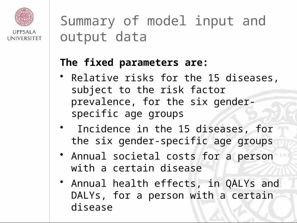
Summary of model input and output data

The fixed parameters are:• Relative risks for the 15 diseases, subject to the

risk factor prevalence, for the six gender-specific age groups

• Incidence in the 15 diseases, for the six gender-specific age groups

• Annual societal costs for a person with a certain disease

• Annual health effects, in QALYs and DALYs, for a person with a certain disease

Summary of model input and output data

The input parameters are:• Number of population, for the six gender-

specific age groups• Current prevalence of the four risk factors in the

six gender-specific age groups, expressed in percent

• Desired prevalence of the four risk factors in the six gender-specific age groups, expressed in percent

Summary of model input and output data

The model outputs for the 5 year horizon:• Changes in number of incident cases, in year 5• Changes in societal costs, total as well as per sector,

in year 5• Changes in health effects, in QALYs and DALYs, in

year 5

The model outputs for the n-year horizon (n=6 to 10):• Changes in number of incident cases, accumulated

from year 5 to year n• Changes in societal costs, total as well as per sector,

accumulated from year 5 to year n• Changes in health effects, in QALYs and DALYs,

accumulated from year 5 to year n

RHS-model as a computer application!

Strengths

• Can include as many diagnoses as we have data for:– Incidence– Risk factors and RR– Costs

• Easy to understand and to use, can be applied to local data

Limitations

• Based on the population at baseline, should include population prognosis

• Time aspect, more careful estimation

• Some risk factors significantly correlate, overestimation

• The model estimates only reduction in morbidity incidence, changes in life style affect morbidity prevalence, underestimation

Conclusions

• The decrease in the prevalence of risk factors can result in cost savings for the society

This model can be adapted to different

populations by taking into account the existing

age structure and the prevalence of risk factors

The model can be extended/adapted for

different diagnoses and risk factors

Development plans

• To include the population prognosis function

• More risk factors?• Web-based application, PC and Mac• ???

P.S. Similar models:

• Dutch RIVM model (Feenstra et al, 2011)• Australia (Cadilhac et al, 2011)