COMMON VALUE ALL-PAY AUCTIONS

Chang-Koo Chi Pauli Murto Juuso Valimaki∗

Department of EconomicsAalto University School of Business and HECER

November 29, 2015

Abstract

This paper analyzes all-pay auctions where the bidders have a common value for the objectfor sale and where the signals take finitely many values. We show that even with affiliatedsignals, it is quite common that monotonicity of symmetric equilibria fails in the sense thatbidders with higher signals do not always win over those with lower signals. We show thatrent equalization is surprisingly common for these games and hence the expected revenue thatthe seller can raise by such auctions is high. We also briefly investigate another non-standardauction format where losing bidders make payments: the war of attrition.

JEL CLASSIFICATION: D44, D82KEYWORDS: All-pay auctions, war of attrition, common values, affiliated signals

1. Introduction

This paper analyzes all-pay auctions under the assumption that the bidders have a common valu-ation for the good that is sold, but asymmetric private estimates of this value. This paper providesthe first steps towards understanding two interlinked features of such models. We look for con-ditions characterizing when bidding is monotone in the sense that bidders with more optimisticbeliefs about the value of the good always win against more pessimistic bidders. Secondly, we askwhen more optimistic bidders obtain positive rents in equilibrium. Our analysis also enables usto compare the equilibrium expected revenue in all-pay auctions to the expected revenues arisingin standard formats such as first-price and second-price auctions. Throughout the analysis, weconcentrate on symmetric Bayesian Nash equilibria.

An all-pay auction has a fixed set of bidders that compete for a fixed prize by submitting simul-taneous bids under the rule that the highest bidder wins and all bidders (regardless of whether

∗Chi: chang-koo.chi@aalto.fi, Murto: pauli.murto@aalto.fi, Valimaki: juuso.valimaki@aalto.fi

1

they win or not) must pay their bid. Even though auctions with such rules are seldom conducted,this format is viewed as an interesting one because of its theoretical connection to models ofwinner-takes-all contests where bidders take the role of contestants expending resources to win afixed prize (e.g., Hillman and Riley (1989) and Baye et al. (1993)). Such models have been exten-sively analyzed under the assumption of common knowledge of the payoffs of the bidders, andalso in the case where the bidders have imperfect information on their private value of the object.

In many contest situations, it is natural to assume that the value of the prize is common toall contestants, but each contestant has an imprecise estimate of this value. Examples includelobbying for a policy with uncertain economic effects or a contest for a rent-generating positionwith uncertainty about the size of the rent. A common value all-pay auction of a single-objectprovides a simple model where such economic problems can be analyzed.

Surprisingly, little is known about equilibrium bidding in common value auctions under all-pay rules. It is quite likely that the difficulty of analyzing such auctions reflects the difficulty ofestablishing the existence of an equilibrium in monotone strategies, i.e. strategies where bidderswith higher signals (i.e. higher estimates of the value of the object) submit higher bids. An earlycontribution by Krishna and Morgan (1997) derives sufficient conditions for the existence of asymmetric pure strategy equilibrium in monotone strategies. Unfortunately, the conditions arevery strong and furthermore not easily verified in terms of the primitives of the model. A recentpaper by Siegel (2014) analyzes a model with a finite set of possible signals on the value of theprize, and derives conditions for the existence of a monotonic mixed strategy equilibrium. Inthese equilibria, a bidder with a higher signal always wins against any bidder with a lower signal.

In our analysis, we keep the assumption of finite signals but we do not restrict attention tomonotone equilibria. With a finite number of bidder types, we can characterize equilibrium bid-ding in mixed strategies using familiar tools from games with discontinuous payoff functions asin capacity constrained pricing games. For the case where bidding is in non-monotone strategies,we do not know how to characterize equilibrium bidding if there is a continuum of signals.

We concentrate on the case where the true value of the prize is a binary random variable andthe signals are correlated with the value, but independent across bidders conditional on the value.We characterize the symmetric equilibria and find that monotone equilibria arise only under aquite limited range of parameters of the model. Our main focus is on determining when biddersearn a positive equilibrium rent in the symmetric equilibrium of the model. We show that under awide range of parameter values, rent dissipation holds in full. Even the bidders with the highestrealized signals compete away all their information rent. This is in sharp contrast with the con-clusion that obtains when monotone equilibrium exists (or with private values uncertainty in themodel). From a theoretical perspective, this finding is of some interest since it shows that the rev-enue to the auctioneer is the highest possible that can be achieved in an incentive compatible andan individually rational mechanism. This expected revenue also strictly dominates the expectedrevenue of other well-known auction formats such as first-price auction or second-price auction.1

1Focusing on a pure-strategy symmetric monotone equilibrium, Krishna and Morgan (1997) compare the expectedrevenue to the auctioneer in all-pay and first-price auctions and show that all-pay auctions are revenue-superior to

2

To get an idea why rent dissipation might hold in equilibrium, consider the case with a bi-nary signal. Suppose for starters that bidding is in monotone strategies and therefore the bidderswith more optimistic beliefs (those who observed the high signal) about the value of the goodalways win against the more pessimistic bidders (those who observed the low signal). Under theassumption that bidders’ signals are affiliated, however, bidders with high signals believe thatthey are more likely to face a competitor that has seen a high signal. Hence it follows that whilebidders with high signal are optimistic about the quality of the good, they are pessimistic aboutthe state of competition in the market: their expected level of competition is higher than the levelof competition that the low-signal bidders expect.

Up to this point in the discussion, we have not considered the auction format at all and hencethe reasoning above applies to standard auction formats as well. To understand why monotonicityfails under all-pay rules but not under standard rules, consider a first-price auction. In this case,a bidder makes a payment only if she wins the auction. With all-pay rules to the auction, a hightype bidder that submits the lowest bid in the equilibrium support of the high-type bidder makesa loss with probability one if the competing bidder is also of a high type. In standard auctions,this loss is not present and hence high-type bidders always outbid the low-type bidders.2

All-pay auctions are not the only auction format where losing bidders end up making pay-ments. Many competitive situations are naturally modeled as wars of attrition where the con-testants expend resources until all but one contestants have given up and the remaining playerwins the resource. In the last section of this paper, we consider the simplest war of attrition wheretwo players with binary signals compete for a resource whose true value is drawn from a binarydistribution. We model the war of attrition as a second-price all-pay auction as is common in theliterature. We show that the expected revenue in the war of attrition exceeds (weakly) the expectedrevenue of the all-pay auction (and hence also first- and second-price auctions).

The paper contributes to the auction and contest theory literature in that all-pay auctions lie intheir intersection.3 The early literature of all-pay auctions has generally focused on environmentswhere bidders have complete information about each player’s value of the object and cost of bid-ding (e.g., Hillman and Riley (1989) and Baye et al. (1993)). Siegel (2009) provides a definitivetreatment of this model, by allowing heterogeneity on the bidder’s characteristics, and character-izes the bidder’s expected payoff in equilibrium in terms of his power. Our payoff characterizationresult—Theorem 1 in Section 5—gives a similar flavor, but the key difference lies in the definitionof each bidder’s power.

first-price auctions.2The standard proof of existence of a monotone pure strategy Nash equilibrium in a Bayesian game relies on the

single-crossing condition developed by Athey (2001), which requires that if his opponents employ a nondecreasingbidding strategy, the incremental return of a bidder from placing a high bid rather than a low bid satisfies the single-crossing property in his type. In the all-pay auction with interdependent value, even when bidders’ signals are affili-ated, the condition does not hold. As a matter of fact, the monotonicity condition, exploited by Krishna and Morgan(1997) and subsequent works, is a sufficient condition for the all-pay auction game to satisfy the single-crossing condi-tion.

3An all-pay auction corresponds to a contest with the success function where the prize is awarded to the contestantwho put forth the greatest effort. The recent survey paper by Kaplan and Zamir (2015) gives a comprehensive pictureof recent developments in the auction and contest theory.

3

The literature of all-pay auctions with incomplete information has developed by relaxing theassumptions of the revenue equivalence theorem. However, in contrast with this paper, most ofthat literature has only considered monotone strategy equilibria (MSE).4 Amann and Leininger(1996) study the two-bidder case with independent private values but asymmetric distributions,and characterize a unique MSE.5 Krishna and Morgan (1997) derive a symmetric monotone pure-strategy equilibrium from the model with symmetric interdependent values and affiliated signalsa la Milgrom and Weber (1982).6 However, as it has been pointed out earlier, such an equilibriumexists under a restrictive monotonicity condition. Developing a discrete version of monotonicitycondition, Siegel (2014) provides a way to construct a monotone mixed-strategy equilibrium inthe asymmetric environment. The symmetric common value environment in our paper allows usnot only to derive a non-monotone strategy equilibrium but to establish a link between existenceof a MSE and rent dissipation through the payoff characterization theorem.

The paper is also related to auctions with entry costs. A recent paper by Murto and Valimaki(2015) compares the expected revenue in first- and second-price common value auctions whenprior to the auction stage, the bidders make a costly entry decision. The connection to the currentnon-standard auction forms comes from the observation that the total payment by losing biddersis positive even in these standard auction formats once we account for the entry cost.

We start with the simplest case of a two-bidder model with two possible signals. The resultsgeneralize easily to a model with N bidders with two signals. We also consider the two-biddermodel with M signals. This allows us to give easily interpretable conditions for the existenceof monotone equilibria and also for the case where full rent dissipation holds. The last sectionconsiders the binary model of war of attrition.

2. The Model

We set up the model in sufficient generality to cover all the remaining sections where we analyzevarious special cases of this model. The value of the single indivisible object is determined by arandom variable θ (which we also refer to as the state) with a finite support Θ = {θ1, · · · , θS} ⊂ <,and denote by q ∈ ∆(Θ) a common prior. The common value of the object in state θ is givenby v (θ) for all risk-neutral bidders i ∈ {1, ..., N}. The bidders are privately informed about θ asfollows: each i observes a conditionally i.i.d. signal ti with a common finite support Ti = T ≡{t1, · · · , tK} ⊂ <. Let αs(k) ≡ Pr(ti = tk|θ = θs) denote the information structure of the model.

4To the best of our knowledge, one exception is Turocy and Rentschler (2014) who study the symmetric environmentwith general affiliated valuations and two bidders, but focus on an algorithm to compute equilibria including non-monotonic ones. Our paper focuses on the common value case but gives a full characterization of the expected payoffin equilibrium as well as a systematic link to the existence of MSE.

5Parreiras and Rubinchik (2010) find that in the same environment with more than two bidders (possibly risk-averse), the monotone strategy equilibrium exhibits an ”all-or-nothing” feature. In particular, a bidder may completelydrop out by bidding zero even though he has a chance of winning.

6McAdams (2007) finds that the symmetric equilibrium of Krishna and Morgan (1997) is unique among the set ofmonotone pure-strategy equilibria (MPSE). More precisely, there is no asymmetric MPSE in symmetric all-pay auctions.Note that this uniqueness result does not apply to our model, because all-pay auctions with finite signals give rise toequilibrium in mixed strategies and we analyze non-monotone strategy equilibrium as well.

4

Throughout the paper, we assume that the model satisfies the monotone likelihood ratio property:for all tk′ > tk and θs, the likelihood ratio αs(k′)

αs(k) is increasing in s.The bidders i submit simultaneously a bid bi ≥ 0 and a bidder with the highest bi receives the

object. If two or more bidders are tied for the highest bid, then the object is allocated based on thesymmetric randomization rule. This does not happen with positive probability in any BNE of thegame. Regardless of who wins the auction, all bidders pay their bids. When the state of the worldis θ, the ex post payoff to bidder i at bid profile b = (b1, ..., bN) can be written as

ui (b, θ) =N−1

∑n=0

1n + 1

v (θ) 1Wni(b)− bi,

where for each n ∈ {0, 1, · · · , N − 1}, Wni ≡ {b|bi ≥ bj for all j, and bi = bj for n different j 6= i}

denotes the set of bid profiles such that bi is the highest bid and bidder i is tied with n differentopponents.

At the moment of bidding, the value v (θ) is uncertain and each bidder i has statistical infor-mation on θ only through ti. Hence the bid must be a function of ti only. It should come as nosurprise that in this finite type setting, we must consider mixed strategies. Hence we let σk

i denotethe mixed strategy by bidder i that has observed signal tk and supp[σk

i ] denote its support. We letσi =

(σ1

i , ..., σKi). We shall also make use of the c.d.f. Fk

i (b) that gives the probability that bidder iwith signal tk submits a bid bi that is no larger than b.

Since we have a model with common values, it is important that when choosing their bids,each i considers the expected value of the object conditional on her own signal and conditionalon the event of winning the auction. This latter conditioning obviously depends on the strategieschosen by all bidders in the auction. Hence we write the expected payoff for bidder i with signaltk when the other bidders employ strategies σ−i as:

vi

(bi, tk; σ−i

)=

N−1

∑n=0

Pσ−i (Wni )E

[v (θ)n + 1

∣∣∣ti = tk, Wni ; σ−i

]− bi,

where Pσ−i indicates the probability measure on <N−1 induced by σ−i.We can now define the Bayes Nash equilibrium for our game.

DEFINITION 1. A Bayes Nash equilibrium (BNE) of the all-pay auction is a vector of strategies σ =

(σ1, ..., σN) such that for all i, all k, and all bi ∈ supp[σki ], we have

bi ∈ argmaxb

vi

(b, tk; σ−i

).

A BNE is said to be symmetric if for all i, j, σi = σj. We denote by σ∗ = (σ1∗ , · · · , σK

∗ ) thesymmetric BNE strategy with the subscript ∗ rather than the index of bidders. Similarly, we denoteby F∗ = (F1

∗ , · · · , FK∗ ) the corresponding bid distribution function to σ∗. In this paper, we analyze

the symmetric BNE of the all-pay auction. Note that a symmetric BNE is characterized by either aprofile of strategies σ∗ or a vector of bid distribution functions F∗.

5

3. Binary Model

In this section, we restrict attention to the simplest model of all-pay auctions with common values,which shows the cleanest version of our result. We consider the symmetric binary all-pay auctionbetween two bidders, where each bidder i ∈ {1, 2} receives a signal ti which conveys partialinformation about the unknown state θ ∈ {L, H}. θ = H indicates the state where the value of theobject is high and L indicates the state where the value is low. We assume v(H) > v(L) ≥ 0. Wedenote the prior probability of the state being H by q = Pr{θ = H}.

Each bidder i observes an imperfect but informative signal (or type) ti ∈ {t1, t2}. Let Pr{ti =

t2|θ} = αθ ∈ (0, 1) for each θ. We assume throughout the paper that the signal structure satisfiesthe monotone likelihood ratio property (MLRP). In this binary information structure, the MLRPimplies αL ≤ αH. In the current model with just two states, the assumption of MLRP is withoutloss of generality.

The bidder i’s (mixed) strategy is then represented by σi : {t1, t2} → ∆(R+). For each k =

{1, 2}, we denote by

Fki (b) := Pr{his bid is less than or equal to b|ti = tk}

the bid distribution function associated with σki .

Since there are only two bidders, we can express the expected value of the object conditionalon the pair of signals

(ti, tj

)as v(k, m) ≡ E

[v(θ)|ti = tk, tj = tm] for k, m ∈ {1, 2}. It is also useful

to denote the probability that bidder i with signal tk assigns to her opponent being of type tm bypk(m) ≡ Pr{tj = tm|ti = tk}. It is a routine task to express v (k, m) and pk (m) in terms of theprimitives 〈q, αH, αL, v(H), v(L)〉 using Bayes rule.

Given her opponent’s strategy σj = (σ1j , σ2

j ), bidder i’s expected payoff conditioned on her bidb and type tk can be written

v(b, k; σj) = E[v(θ)1{i wins at b}|ti = tk

]− b

=2

∑m=1

v(k, m)pk(m)Fmj (b)− b

=2

∑m=1

φ(k, m)Fmj (b)− b

where we let φ(k, m) := v(k, m)pk(m).In this binary model, a symmetric BNE of the auction is given by two cumulative distribution

functions F1∗ (·) and F2

∗ (·) over equilibrium bids by bidders of type t1and t2, respectively. The fol-lowing easy (and unsurprising) lemma records the basic properties of these distributions. Noticethat all of the arguments in the lemma can easily be extended to the case where we have multiplesignals, multiple states or multiple bidders.

LEMMA 1. In any symmetric BNE(

F1∗ , ..., FK

∗)

of the all-pay auction, the following properties hold:

6

1. For each k, Fk∗ is continuous, i.e. neither distribution has mass points.

2. The union of the supports ∪k supp[Fk∗ ] is a connected interval beginning at 0.

Proof.

1. By the full support assumption for all signals, a bid of b′ results in a tie with a strictly positiveprobability πk (b′) if Fk

∗ has a mass point at b′ for some k. But then raising the bid to b′ + ε isa profitable deviation whenever ε < 1

2 πk (b′) v (L) . Hence there cannot be any mass points.

2. Assume to the contrary that there is a bid b′ /∈ ∪k supp[Fk∗ ] and mink{Fk

∗ (b′)} < 1. Let

b∗ = min{

b ≥ b′∣∣∣b ∈ ∪k supp[Fk

∗ ]}

.

Then a deviation from b∗ to b′ reduces the payment by b∗ − b′ > 0 while not affecting theprobability of winning the auction. This contradicts with b∗ ∈ ∪k supp[Fk

∗ ].

The next lemma shows that the low bidders start bidding at arbitrarily low bids. This allows usto conclude that the bidders with low signals receive no rent in equilibrium (as one would expect).

LEMMA 2. In every symmetric BNE of the all-pay auction, 0 ∈ supp[F1∗ ] and that supp[F1

∗ ] is connected.

Proof. Let b′ /∈ supp[F1∗ ]. Then by Lemma 1, b′ ∈ supp[F2

∗ ] and therefore by the indifferencecondition of the type t2 bidder, we have

φ (2, 2) f 2∗(b′)= 1,

where f 2∗ is the density of F2

∗ . But then

φ (1, 2) f 2∗(b′)=

φ (1, 2)φ (2, 2)

< 1,

since v (H) > v (L) and since MLRP holds.But this means that

∂v (1, b; σ)

∂b

∣∣∣∣b=b′

< 0

for all b′ such that b′ ∈ supp[F2∗ ], and b′ /∈ supp[F1

∗ ]. Hence it is not optimal for the bidder withsignal t1 to place any bid b ≥ b′. This implies immediately that supp[F1

∗ ] is connected and that0 ∈ supp[F1

∗ ].

A similar argument shows that the support of F2∗ is also connected.

LEMMA 3. If φ(2, 1) ≥ φ(1, 1), then supp[F1∗ ] ∩ supp[F2

∗ ] = ∅. If φ(2, 1) < φ(1, 1), then supp[F1∗ ] ∩

supp[F2∗ ] = supp[F1

∗ ] .

7

Proof. If b′ /∈ supp[F2∗ ], then φ (1, 1) f 1

∗ (b′) = 1, and therefore

∂v (2, b; σ)

∂b

∣∣∣∣b=b′

=φ (2, 1)φ (1, 1)

.

Hence it is never optimal for type t2 bidder to bid below any bid in the support of type t1 only bid-der if φ(2,1)

φ(1,1) > 1 . In the light of the previous lemma, this leaves open the possibility of consecutivenon-overlapping supports for the two bidders.

If φ(2,1)φ(1,1) < 1, then a bidder with signal t2 never submits bids that above b ∈ supp[F∗1] ∩(

supp[F2∗ ])C. In light of the previous two lemmas, the only possibility then is that the supports

are overlapping. In this case, the first order conditions for optimality give the following equationsystem:

φ (1, 1) f 1∗ + φ (1, 2) f 2

∗ = 1,

φ (2, 1) f 1∗ + φ (2, 2) f 2

∗ = 1.

Hence

f 1∗ =

φ (1, 2)− φ (2, 2)φ (1, 2) φ (2, 1)− φ (1, 1) φ (2, 2)

,

f 2∗ =

φ (2, 1)− φ (1, 1)φ (1, 2) φ (2, 1)− φ (1, 1) φ (2, 2)

.

The MLRP and v (H) > v (L) imply that φ (1, 2) < φ (2, 2). Hence we see that(

f 1∗ , f 2∗)≥ (0, 0) if

and only if φ (2, 1) < φ (1, 1) . This also shows that it is impossible to have overlapping supportswhen φ (2, 1) ≥ φ (1, 1) .

The only remaining thing to show is that when φ (2, 1) < φ (1, 1) , we have supp[F1∗ ] ⊂

supp[F2∗ ]. To see this, note from the above equations that

f 1∗

f 2∗=

φ (2, 2)− φ (1, 2)φ (1, 1)− φ (2, 1)

.

Some tedious but straightforward algebra allows us to write this ratio in terms of the primitivesof the model as follows;

φ (2, 2)− φ (1, 2)φ (1, 1)− φ (2, 1)

=v (H) αH − v(L)αL

v (H) αH − v(L)αL − (v (H)− v (L))> 1.

Hence if supp[F1∗ ] = [0, B1] and supp[F2

∗ ] = [0, B2], then B1 < B2 and the claim follows.

When we write φ(2, 1) and φ(1, 1) in terms of the primitives of the model, we get the followingcondition for φ(2, 1) ≤ φ(1, 1) :

v(H)

v(L)≤ 1− αL

1− αH .

8

1

<b20 b1

F1∗ (b)

F2∗ (b)

(a) φ(2, 1) ≥ φ(1, 1)

1

<B20 B1

F1∗ (b)

F2∗ (b)

(b) φ(2, 1) < φ(1, 1)

Figure 1: Symmetric Equilibrium F∗ = (F1∗ , F2∗ ) in the Binary Model

In their words, we need that the value of the good is not too different across the two states oralternatively the likelihood of signal t1 should be much smaller in state H than in state L. Underthese conditions, the all-pay auction displays complete rent dissipation. Since the support of bothbidders extends to zero, we see that even the more optimistic bidder gets a zero expected payoffin equilibrium since a bid of zero has a zero probability of winning.

We collect the results in the following proposition that gives a full characterization of thesymmetric equilibria of the all-pay auction.

PROPOSITION 1. The all-pay auction has a unique symmetric equilibrium with the following properties.

1. If φ(2, 1) ≥ φ(1, 1), then the unique symmetric equilibrium (F1, F2) = (F∗, F∗) is

F1∗ (b) =

0 for b < 0,

bφ(1,1) for b ∈ [0, b1],

1 for b > b1

F2∗ (b) =

0 for b < b1,

bφ(2,2) − φ (1, 1) for b ∈ [b1, b2],

1 for b > b2,

where b1 = φ(1, 1) and b2 = φ(1, 1) + φ(2, 2).

2. If φ(2, 1) < φ(1, 1), then the unique symmetric equilibrium (F1, F2) = (F∗, F∗) is

F1∗ (b) =

0 for b < 0,

φ(2,2)−φ(1,2)φ(1,1)φ(2,2)−φ(2,1)φ(1,2) b for b ∈

[0, B1

],

1 for b > B1

F2∗ (b) =

0 for b < 0,φ(1,1)−φ(2,1)

φ(1,1)φ(2,2)−φ(2,1)φ(1,2) b for b ∈[0, B1

],

bφ(2,2) −

φ(1,1)−φ(2,1)φ(2,2)−φ(1,2) for b ∈

[B1, B2

],

1 for b > B2,

9

where B1 = φ(1,1)φ(2,2)−φ(2,1)φ(1,2)φ(2,2)−φ(1,2) and B2 = φ(2, 1) + φ(2, 2).

Our last result in this section concerns the revenue ranking between all-pay auction and thestandard first-price and second-price auctions.

PROPOSITION 2. The symmetric equilibrium of the all-pay auction generates a higher revenue that thesymmetric equilibria of the first-price or second price auctions.

Proof. Since we have a common value auction, it is sufficient to compare the expected payoffs tothe bidders across the various auction formats. In first-price and second-price auctions, the bidderwith signal t1 has a zero expected payoff just as in the all-pay auction. Hence all the revenuedifferences result from differences in t2 bidder’s payoffs.

In the ex post equilibrium of the second-price auction, b(tk) = v (k, k) for k ∈ {1, 2}. Hence the

expected payoff to t2 is simply p2 (1) (v (2, 1)− v (1, 1)) . In the symmetric equilibrium of the firstprice equilibrium, b

(t1) = v (1, 1) and the bidder of type t2 plays a mixed strategy with support

starting at v (1, 1) . Hence her expected payoff is the same as in the second price auction since abid at v (1, 1) + ε gives the same payoff in the limit as ε→ 0.

If φ(2, 1) < φ(1, 1), then t2 gets a zero expected payoff in the all-pay auction and the resultfollows. If φ(2, 1) > φ(1, 1), then the equilibrium payoff of t2 is given by

p2 (1) v (2, 1)− φ (1, 1) = p2 (1) v (2, 1)− p1 (1) v (1, 1)

< p2 (1) (v (2, 1)− v (1, 1))

since by MLRP, p1 (1) > p2 (1) .

We have been perhaps overly pedantic in the arguments in this section. The reason for this isthat in the sections to follow, we extend our results to cover many players, many signals and manystates. We shall use similar reasoning as above but we will omit some details where the argumentsare similar to those above.

4. Many Players

In this section, we maintain the structure from the previous section, but we allow the numberof participants in the auction to be any integer N. Our aim here is to show that the likelihoodof monotone equilibria decreases as the number of players grows. The previous literature hasfocused to a large extent on the monotone equilibria. The results in this section indicate that atleast for the binary signal case, the non-monotone equilibria deserve some attention.

For each n ∈ {0, 1, · · · , N − 1}, we define

v(k, n) = E[v(θ)|t1 = tk, # of bidders with t2 among his opponents = n

]as bidder 1’s expected value conditioned on his type and the event that he faces n high-typeopponents.

10

Let pk(n) denote her interim belief of such event, i.e.,

pk(n) = Pr{

# of bidders with t2 among his opponents = n∣∣ t1 = tk

}.

Define the following function φ : N → R by

φ(n) := v(2, n)p2(n)− v(1, n)p1(n).

Notice the similarity of φ (n) to the expressions φ (2, 1)− φ (1, 1) and φ (2, 2)− φ (1, 2) that wereimportant for characterizing when we can have monotone equilibria in the two-bidder case.

In order to simplify the presentation, we assume further that αH = α > 12 , and αL = 1− α.7

Under this assumption, simple but tedious algebra shows that

sgn[φ(n)] = sgn

[v(H)

v(L)−(

α

1− α

)N−1−2n]

.

From this formula, we can deduce two properties of φ: (1) φ(N − 1) > 0 and (2) the strictsingle crossing property (SCP) of φ, i.e.,

φ(n) ≥ 0 implies φ(n′) > 0 ∀ n′ > n.

Since α > 1/2, note that as N grows large enough, φ(n) is likely to be negative.The following lemma gives a further implication of φ(N − 1) > 0. The proof is similar to the

corresponding proof in the two-bidder case and hence is omitted for brevity.

LEMMA 4. Let(σ1∗ , σ2∗)

be a symmetric BNE of the all-pay auction with the corresponding bid distributions(F1∗ , F2∗). Then 0 ∈ supp[F1

∗ ] so there is no information rent for low-type bidders in equilibrium.

The next proposition presents a sufficient (and necessary) condition for the existence of amonotone strategy equilibrium and for bidders of type t2 to earn positive information rent inequilibrium.

PROPOSITION 3. If φ(0) ≥ 0, then the all-pay auction has a unique symmetric BNE. In this equilibrium,supp[F1

∗ ] ∩ supp[F2∗ ] = ∅.

Proof. Since the function φ satisfies the strict SCP, φ(0) ≥ 0 implies φ(n) > 0 for all n = 1, · · · , N−1. Hence we can use an argument similar to Lemma 2 to conclude that the supports must bedisjoint in equilibrium. The monotone strategy equilibrium is characterized in Figure 2-(a).

PROPOSITION 4. If φ(0) < 0, then 0 ∈ supp[F2∗ ] so there is no informational rent for bidders of type t2

in equilibrium.7The details for general (αH , αL) are available upon request from the authors.

11

supp[F1∗ ]

supp[F2∗ ]

0 b1

b2 b2

b1 = b2 = v(1, 0)p1(0)

b2 = b2 + ∑N−1n=1 v(2, n)p2(n)

F1∗ (b) =

[b/b1

]N−1

F2∗ solves ∑N−1

n=0 v(2, n)p2(n)[F2∗ (b)]n = b + φ(0)

(a) Case1: φ(0) ≥ 0

supp[F1∗ ]

supp[F2∗ ]

0 B1

0 B2

B1 solves B1 =N−1

∑n=0

φ(n)[F2∗ (B1)]

n

B2 =N−1

∑n=0

v(2, n)p2(n) > B1

(b) Case 2: φ(0) < 0

Figure 2: Characterization of Symmetric Equilibrium F∗ in all-pay auctions with many participants

Proof. Suppose min{supp[F2∗ ]} = b > 0. Since the union of the supports is connected by Lemma

1, we must have F1∗ (b) > 0 in this case. Also, since bidding such b is indifferent to bidding 0 for

low-type bidders by Lemma 4, it must be the case that

b =N−1

∑n=0

v(1, n)p1(n)[F1∗ (b)]

N−1−n[F2∗ (b)]

n = v(1, 0)p1(0)[F1∗ (b)]

N−1.

However, the expected payoff of high-type bidders from making the bid b is then

u(b, 2|σ∗) =N−1

∑n=0

v(2, n)p2(n)[F1∗ (b)]

N−1−n[F2∗ (b)]

n − b = φ(0)[F1∗ (b)]

N−1 < 0,

which contradicts to b ∈ supp[F2∗ ]. Hence 0 ∈ supp[F2

∗ ].

We complete this section by showing that the analogue of Lemma 2 holds, both supp[F1∗ ] and

supp[F2∗ ] are a connected interval, and supp[F1

∗ ] is included in supp[F2∗ ]. The equilibrium with

overlapping supports is depicted in Figure 2-(b).

PROPOSITION 5. Suppose φ(0) ≤ 0. In any symmetric BNE of the all-pay auction, both supp[F1∗ ] and

supp[F2∗ ] are a connected interval.

Proof. Suppose not. Then there is a closed interval [b1, b2] such that supp[F1∗ ] ∩ [b1, b2] = {b1, b2}.

By Lemma 4, both b1 and b2 have an alternative expression:

b1 =N

∑n=0

v(1, n)p1(n)(

N − 1n

)[F1∗ (b1)]

N−1−n[F2∗ (b1)]

n

b2 =N

∑n=0

v(1, n)p1(n)(

N − 1n

)[F1∗ (b1)]

N−1−n[F2∗ (b2)]

n,

where we used F1∗ (b1) = F1

∗ (b2) for the expression of b2. Also, it follows from Lemma 1 and 4 that

12

b1 ∈ supp[F2∗ ] and the expected payoff from making b1 must be zero to high-type bidders, namely,

u(b1, 2|σ∗) =N

∑n=0

v(2, n)p2(n)(

N − 1n

)[F1∗ (b1)]

N−1−n[F2∗ (b1)]

n − b1

=N

∑n=0

φ(n)(

N − 1n

)[F1∗ (b1)]

N−1−n[F2∗ (b1)]

n = 0.

Observe that the expression φ(n)(N−1n )[F1

∗ (b1)]N−1−n[F2

∗ (b1)]n also satisfies the strict SCP in n. This

means that

u(b2, 2|σ∗) =N

∑n=0

φ(n)(

N − 1n

)[F1∗ (b1)]

N−1−n[F2∗ (b2)]

n

=N

∑n=0

φ(n)(

N − 1n

)[F1∗ (b1)]

N−1−n[F2∗ (b1)]

n ·[

F2∗ (b2)

F2∗ (b1)

]n

> 0,

where the inequality comes from the (discrete version) Folk single-crossing lemma and the fact

that[

F2∗ (b2)

F2∗ (b1)

]nis an increasing function in n.8 This implies that the high-type bidder obtains a

strictly positive information payoff by making the bid of b2, which contradicts with the result ofProposition 4. A similar argument can be applied to establish that supp[F2

∗ ] is also connected. Theproof is complete.

We could also show using similar techniques to the previous section that when monotonicequilibria fail to exist, then supp[F1

∗ ] ⊂ supp[F2∗ ]. Our main interest is nevertheless in character-

izing the equilibrium payoffs for the bidders across symmetric equilibria. The conclusions in thecurrent section are exactly as in the previous section. It is worth observing that for any fixed α, thepossibility of having a monotonic equilibrium vanishes as n grows large enough. For example atα = 2

3 , and n = 4, a monotone strategy equilibrium exists only if v (H) > 8v (L) .

5. Two Bidders with Many Signals

In this section, we extend the analysis to cover the case with two bidders, two states and manysignals, ti ∈ {t1, · · · , tK}. Whereas in Section 3, the restriction to two states was for notational ease,here that restriction involves some loss of generality. Unfortunately, the monotone comparativestatics results that we need in this section are not valid in the case of multiple states and we havenot been able to analyze the general case of many signals and many states.

We derive an intuitive characterization for the symmetric equilibria of the all-pay auction. Weshow that the different bidder types can be collected into two sets: bidders with low signals earnzero rents while in the other group, the bidders’ expected rent is increasing in their signal. Each

8For a discrete domain N, the single-crossing lemma states that if f : N → < satisfies the (strict) single-crossingproperty and ∑n∈N f (n) = 0, then ∑n∈N f (n)g(n) ≥ (>) 0 for an (strictly) increasing function g : N → <. Note thatthe given properties of f imply ∑n≥k f (n) ≥ 0 for every k. Hence the lemma follows from the fact that every increasingfunction can be approximated by step functions ∑i γi1{n≥ki}.

13

of these groups can be empty and hence full rent dissipation is possible in this case as well. Weregard the results as natural generalizations to those in the binary model.

We write the bidder i’s expected payoff conditional on (i) his type ti = k, (ii) his bid b, and (iii)his opponent’s strategy σj as before:

v(b, k; σj) = E[

v(θ) 1{β j(tj)≤b}(tj)∣∣∣ ti = k

]− b =

T

∑t=1

v(k, t)pk(t)Ftj (b)− b.

We define as before

φ(k, t) := v(k, t)pk(t).

We say that the model satisfies the monotonicity condition when φ(k, t) increases in k for every t,implying that a higher type is always a good news to bidder i regardless of his opponent’s type.It can be shown by simple algebra that for every k > m,

φ(k, t)− φ(m, t) = q(1− q)αH(k)αL(m)− αH(m)αL(k)

p(k)p(m)

[v(H)αH(t)− v(L)αL(t)

].

Due to the MLRP, the expression in the numerator is always nonnegative, and thus the signof φ(k, t)− φ(m, t) is determined by the expression in the bracket, v(H)αH(t)− v(L)αL(t), whichsatisfies the single-crossing property (SCP) in t by MLRP. Consequently, the function φ(k, t) sat-isfies the SCP in (k; t) in the sense that for every k > m, φ(k, t) − φ(m, t) < 0 for t < τ butφ(k, t)− φ(m, t) ≥ 0 for t ≥ τ, where τ indicates the tipping point at which v(H)αH(t)− v(L)αL(t)changes its sign from negative to positive.

It is worthwhile to note that the tipping point τ is not affected by the choice of k > m, andthat the monotonicity condition holds only when τ = 1.9 For future reference, we define τ∗ as thetipping point at which the t-th partial sum,

t

∑s=1

[v(H)αH(s)− v(L)αL(s)

]= v(H)AH(t)− v(L)AL(t) where Aθ(t) ≡

t

∑s=1

αθ(s),

changes its sign from negative to positive. Since the MLRP implies the monotone probability ratioproperty, i.e., AH(t)/AL(t) nondecreasing in t, the above partial sum satisfies the SCP in t as well.It is not difficult to verify that (i) τ∗ ≤ T is well-defined because v(H)AH(T) − v(L)AL(T) =

v(H)− v(L) > 0, (ii) τ∗ ≥ τ, and (iii) for every k > m, the t-th partial sum

t

∑s=1

[φ(k, s)− φ(m, s)] = q(1− q)αH(k)αL(m)− αH(m)αL(k)

p(k)p(m)

[v(H)AH(t)− v(L)AL(t)

]also changes its sign from negative to positive at t = τ∗.

9We should note here that the difficulties for the model with many states arise from the fact that this invariance of τin k, m does not hold in the more general case.

14

We characterize the bidder’s expected payoff in a symmetric equilibrium. For this purpose,we define by Uσ∗(k) the expected payoff of the type-k bidder in a symmetric equilibrium (σ∗, σ∗),namely,

Uσ∗(k) ≡∫ bk

bk

[−b +

K

∑t=1

φ(k, t)Ft(b)

]dFk(b).

We wish to highlight that the next payoff characterization theorem holds in every symmetric equi-librium.

THEOREM 1. In every symmetric equilibrium (σ∗, σ∗) in the all-pay auction, the expected payoff of thetype-k bidder is

Uσ∗(k) = max {0, w(k, τ∗)} ,

where the function w(k, τ∗) represents his power:

w(k, τ∗) ≡k

∑t=1

φ(k, t)−(

τ∗

∑t=1

φ(τ∗, t) +k

∑t=τ∗+1

φ(t, t)

)

Proof. See Appendix A.

The main implication of the payoff characterization theorem comes from the power functionw(k, τ∗). For an illustration, we demonstrate that w(k, τ∗) satisfies the SCP in k and, like the t-thpartial sum above, changes its sign from negative to positive at k = τ∗. To see this, note that fork ∈ {1, · · · , τ∗ − 1},

w(k, τ∗) =k

∑t=1

φ(k, t)−τ∗

∑t=1

φ(τ∗, t) ≤ −τ∗

∑t=1

[φ(τ∗, t)− φ(k, t)] < 0,

as the τ∗-th partial sum is positive. It is easy to check w(τ∗, τ∗) = 0. Lastly, note that for k ∈{τ∗ + 1, · · · , T}, the power function

w(k, τ∗) =k

∑t=1

φ(k, t)−(

τ∗

∑t=1

φ(τ∗, t) +k

∑t=τ∗+1

φ(t, t)

)

=τ∗

∑t=1

[φ(k, t)− φ(τ∗, t)] +k

∑t=τ∗+1

[φ(k, t)− φ(t, t)]

is always positive, since the first τ∗-th partial sum is positive for k > τ∗ and the difference φ(k, t)−φ(t, t) in the second partial sum is positive for every t ∈ {τ∗ + 1, · · · , k}.

Therefore, the theorem implies that the bidder of type k ≤ τ∗ earns no information rents,whereas the bidder of type k > τ∗ enjoys a positive information rent in every symmetric equilib-rium. When the primitive satisfies the monotonicity condition, i.e., when τ = 1, the new tipping

15

point τ∗ also becomes 1. Therefore, except for the lowest type bidder, every bidder earns a posi-tive information rent, leading to a monotone symmetric equilibrium as we will verify in the proof.When τ∗ = T, on the other hand, every bidder obtains zero expected payoff.

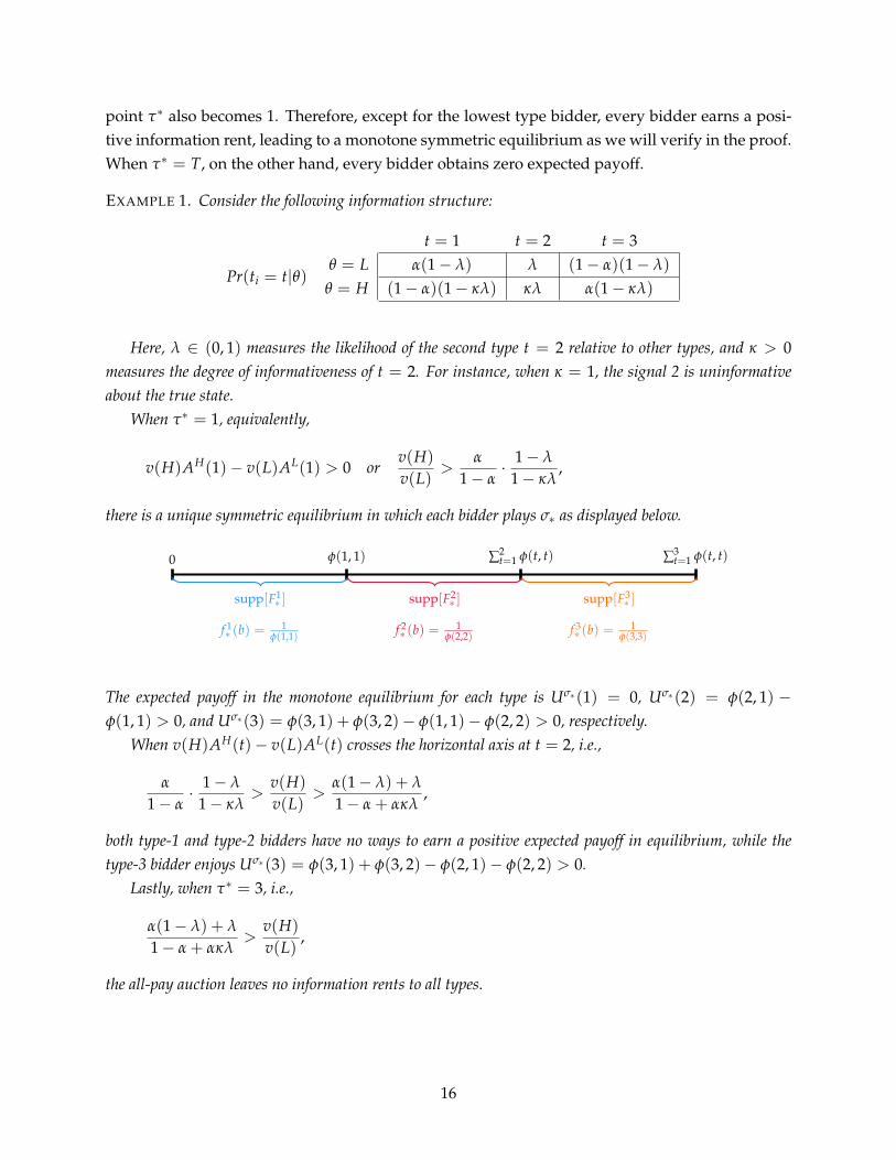
EXAMPLE 1. Consider the following information structure:

t = 1 t = 2 t = 3

Pr(ti = t|θ)θ = L α(1− λ) λ (1− α)(1− λ)

θ = H (1− α)(1− κλ) κλ α(1− κλ)

Here, λ ∈ (0, 1) measures the likelihood of the second type t = 2 relative to other types, and κ > 0measures the degree of informativeness of t = 2. For instance, when κ = 1, the signal 2 is uninformativeabout the true state.

When τ∗ = 1, equivalently,

v(H)AH(1)− v(L)AL(1) > 0 orv(H)

v(L)>

α

1− α· 1− λ

1− κλ,

there is a unique symmetric equilibrium in which each bidder plays σ∗ as displayed below.

0 φ(1, 1) ∑2t=1 φ(t, t) ∑3

t=1 φ(t, t)

supp[F1∗ ] supp[F2

∗ ] supp[F3∗ ]

f 1∗ (b) =

1φ(1,1) f 2

∗ (b) =1

φ(2,2) f 3∗ (b) =

1φ(3,3)

The expected payoff in the monotone equilibrium for each type is Uσ∗(1) = 0, Uσ∗(2) = φ(2, 1) −φ(1, 1) > 0, and Uσ∗(3) = φ(3, 1) + φ(3, 2)− φ(1, 1)− φ(2, 2) > 0, respectively.

When v(H)AH(t)− v(L)AL(t) crosses the horizontal axis at t = 2, i.e.,

α

1− α· 1− λ

1− κλ>

v(H)

v(L)>

α(1− λ) + λ

1− α + ακλ,

both type-1 and type-2 bidders have no ways to earn a positive expected payoff in equilibrium, while thetype-3 bidder enjoys Uσ∗(3) = φ(3, 1) + φ(3, 2)− φ(2, 1)− φ(2, 2) > 0.

Lastly, when τ∗ = 3, i.e.,

α(1− λ) + λ

1− α + ακλ>

v(H)

v(L),

the all-pay auction leaves no information rents to all types.

16

6. War of Attrition

In this last section, we consider a second-price all bid auction also known as war of attrition. Inthis auction, all but the highest bidder pay their own bids. The highest bidder wins the object andpays the second highest bid (again any ties are broken symmetrically). We consider the simplestsetting with two bidders, and binary states and signals.

We show that whenever the war of attrition has a monotone symmetric equilibrium, the all-pay auction with the same payoff and signal structure also has a monotone symmetric equilibrium.Conversely when all rents are dissipated in the symmetric equilibrium of the all-pay auction, thesymmetric equilibrium of the war of attrition also features zero expected payoffs to all bidders.For some parameter values, the all-pay auction has a monotone equilibrium while the war ofattrition displays a new type of equilibrium where the two bid distributions are overlapping butnot nested. In all of these cases, the expected rent of the bidders is smaller in the war of attritionthan in the all-pay auction, and as a result, the expected revenue to the seller is higher in the warof attrition.

Let σi = {σHi , σL

i } for i = {1, 2}. We can write the payoffs for the two bidders i as functions ofthe bids and the state as:

ui(bi, bj, θ

)=

v (θ)− bj if bj < bi,12 v (θ)− bj if bj = bi,

−bi if bj > bi.

Since the true value of the object θ is not known to the bidders when forming their bid, we mustlook at the interim expected payoff

vi

(bi, tk; σj

)= Pσj

(bj < bi

)E[v (θ)− bj

∣∣∣ti = tk, bi < bj; σj ]

+Pσj(bi = bj

) (E

[v (θ)

2

∣∣∣ti = tk, bi = bj; σj

]− bi

)−Pσj

(bi > bj

)bi.

Denote the corresponding bid distributions for the two players by Fki (·) . As before, we let

v(k, m) = E[v(θ)|ti = tk, tj = tm] for k, m ∈ {1, 2}, pk(m) = Pr(tj = tm|ti = tk), and φ (k, m) =

pk (m) v (k, m). Again we concentrate on symmetric equilibria in the game, i.e. on pairs of biddistributions

(F1∗ (b) , F2

∗ (b))

such that for all i, ti and all b ∈ supp[Fk∗ (·)],

b ∈ argmaxb′

vi

(b′, tk; σj

).

Again, it is easy to see by the usual arguments that the distribution functions Fk∗ (·) must be

continuous in any symmetric equilibrium of the game and that the union of the two supports isconnected and starts at zero. Even though the formula for vi

(bi, tk; σj

)looks complicated, notice

17

that a simple perturbation argument of changing the bid of agent i with signal ti from b to b+∆ inthe interior of the support yields a much simpler condition. This change in the bid is payoffrelevant only if bj ≥ b. The hazard rate for the bid of bidder j to lie in [b, b + ∆] if j has observed

signal tj = tm is thenpti (m) f m

∗ (b)∆1−pti (1)F1

∗ (b)−pti (2)F2∗ (b)

and the payoff from from winning at b + ∆ is v (ti, m) .

Notice that the added cost bj − b for bj ∈ [b, b + ∆] is of the order ∆ and hence vanishing incomparison to v (ti, m) for small ∆. Hence the condition for the equalization of the cost (1 per unitof time) and the benefits from the exits by the opponent becomes:

pti (1) f 1∗ (b) v (ti, 1)

1− pti (1) F1∗ (b)− pti (2) F2

∗ (b)+

pti (2) f 2∗ (b) v (ti, 2)

1− pti (1) F1∗ (b)− pti (2) F2

∗ (b)= 1

for all b ∈ int(

supp[Fti∗ (·)])

. This gives a pair of differential equations on that have to be solvedsubject to the relevant boundary conditions.

To see how to solve this pair of equations, consider the parametrized family of linear equationsystems (in ( f 1

∗ , f 2∗ )):

(1)φ (1, 1) f 1

∗ + φ (1, 2) f 2∗ = 1− x,

φ (2, 1) f 1∗ + φ (2, 2) f 2

∗ = 1− x′.

As long as the system on the left hand side has full rank, the pair of equations has a uniquesolution in

(f 1 (x, x′) , f 2 (x, x′)

). Since φ (k, m) > 0 for k, m ∈ {1, 2}, we know that for all x, x′ ∈

[0, 1], at least one of the f i (x, x′) is positive. If both f 1 (0, 0)and f 2 (0, 0) are positive, then we seeimmediately that 0 ∈supp[Fi

∗ (·)] for i = {1, 2}. The necessary and sufficient condition for this isthat:

(φ (1, 2)− φ (2, 2)) (φ (2, 1)− φ (1, 1)) ≥ 0.

Since φ (1, 2) < φ (2, 2), this is equivalent to requiring that

φ (2, 1) < φ (1, 1) .

Notice the similarity here to the analysis of the all-pay auction in Section 3.For this case, we have the initial value conditions F1

∗ (0) = F2∗ (0) = 0, and

(f 1∗ (0) , f 2

∗ (0))=(

f 1 (0, 0) , f 2 (0, 0))

, and we can integrate the system until

b∗ := min{b : max{F1∗ (b) , F2

∗ (b)} ≥ 1 or min{ f 1 (x (b) , x′ (b))

, f 2 (x (b) , x′ (b))} ≤ 0},

where x (b) = p1 (1) F1∗ (b) + p1 (2) F2

∗ (b) , x′ (b) = p2 (1) F1∗ (b) + p2 (2) F2

∗ (b) .It is not hard to show that the binding constraint is that F1

∗ (b∗) = 1. The bid distribution forbids above b∗ follows then from the solution of the complete information war of attrition since ifboth players bid above b∗, then it is common knowledge that both have observed the high signal.

18

If (φ (1, 2)− φ (2, 2)) (φ (2, 1)− φ (1, 1)) < 0, then only the bidder with low signals has b = 0in the support of her bid distribution. This follows from the fact that for affiliated signals, we have

φ (1, 1) + φ (1, 2) ≤ φ (2, 1) + φ (2, 2)

and hence we must have

(φ (1, 2)− φ (2, 2)) < 0 < (φ (2, 1)− φ (1, 1)) .

But as computed in Section 3, we have

φ (2, 1)− φ (1, 1) + φ (2, 2)− φ (1, 2) = (v (H)− v (L)) q(1− q){

αH(1− αL)− (1− αH)αL

p(1) · p(2)

}.

Since

(φ (2, 1)− φ (1, 1)) f 1 (0, 0) + (φ (2, 2)− φ (1, 2)) f 2 (0, 0) = 0,

we can multiply the first equation by f 1 (0, 0) and subtract the second from the first to get

(φ (2, 2)− φ (1, 2))(

f 1 (0, 0)− f 2 (0, 0))

= f 1 (0, 0) (v (H)− v (L)) q(1− q){

αH(1− αL)− (1− αH)αL

p(1) · p(2)

}> 0.

Hence

f 1 (0, 0) > 0 > f 2 (0, 0) .

This implies that 0 ∈ supp[F1∗ (·)] but 0 /∈ supp[F2

∗ (·)]. By comparison to our earlier results,there is a close connection between the two auction formats. If φ (2, 1) < φ (1, 1) , then the supportsof the two types of bidders overlap for small values of b. While the densities take a differentshape in the two auctions (uniform densities for the all-pay auction and densities consistent withconstant hazard rates for the war of attrition), the two cases are similar in the sense that both biddistributions have connected support.

When φ (2, 1) > φ (1, 1) , the situation is somewhat different. In the all-pay auction, the systemof equations that must be solved is essentially the same system as depicted in (1). In the war ofattrition, the right hand side of the equation system changes at we move to higher values of b.Hence it is possible that even if the solution to (1) at (x, x′) = (0, 0) yields f 1 (0, 0) > 0 > f 2 (0, 0) ,the system has positive solutions at different values of (x, x′) .

In order to investigate if this is of consequence in the current war of attrition, consider thefollowing algorithm. Solve the bid distribution of the bidder with signal 1 from the differential

19

supp[F1∗ ]

supp[F2∗ ]

0 b1

b2

b1 = b2 = v(1, 1) ln[p1(2)]−1

F1∗ (b) = 1 +

1p1(1)

[p1(2)− exp

(− b

v(1, 1)

)]F2∗ (b) = 1− exp

(− b

v(2, 2)

)

Figure 3: Characterization of Monotone Strategy Equilibrium F∗ in the war of attrition - When φ(2, 1) >p2(2)p1(2)

φ(1, 1), a monotone strategy equilibrium exists.

equation

φ (1, 1) f 1∗ (b) = 1− p1 (1) F1

∗ (b)

with initial value condition F1∗ (0) = 0. Let F1 (b) denote this solution. The solution is valid until b

such that F1(

b)

.Consider next the system

φ (1, 1) f 1∗ + φ (1, 2) f 2

∗ = 1− p1 (1) F1 (b) ,

φ (2, 1) f 1∗ + φ (2, 2) f 2

∗ = 1− p2 (1) F1 (b) .

for all b ∈ [0, b]. If f 2(

p1 (1) F1 (b) , p2 (1) F1 (b))

for all b ∈ [0, b], then the symmetric equilibriumbid distributions in the war of attrition have non-overlapping supports much as in the all-payauction.

Let bm = min{

b ≤ b : f 2(

p1 (1) F1 (b) , p2 (1) F1 (b))= 0

}. Then the solution is given by

F1∗ (b) =

F1 (b) for b ∈ [0, bm],

F1 (b) for b ∈ [bm, b∗],

1 for b ≥ b∗F2∗ (b) =

0 for b ∈ [0, bm],

F2 (b) for b ∈ [bm, b∗],

F2 (b) for b ≥ b∗.

Here(

F1 (b) , F2 (b))

denotes the solution to (1) in the appropriate range with initial condition(F1 (bm) , F2 (bm)

)=(

F1 (bm) , 0)

and F2 (b) solves

φ (2, 2) f 2∗ (b) = 1− p2 (2) F2

∗ (b)− p1 (1)

with initial condition F2∗ (b∗) = F2 (b∗) .

Given the explicit solution to the auction under war of attrition rules, it is easy to compare theexpected revenue to the all-pay auction. In fact, we formally prove in Appendix B that the war of

20

attrition generates a higher expected revenue than the all-pay auction and as a result, also a higherexpected revenue than first- or second-price auctions.

7. Conclusion

In this paper, we have taken the first steps towards analyzing auctions where losing bidders alsopay. Extending the informational set-up to include many states as well as many signals seemslike an important generalization. Of course, the characterization of equilibria with a continuum ofsignals in the non-monotonic case is a completely open problem.

The motivation for all-pay auctions and wars of attrition comes largely from the literature oncontests, and it would be interesting to extend our analysis towards more general contests. Firstof all, one should consider cases where the winner-takes-all assumption is not as sharp as in thetwo types of models that we analyzed. Second, it would be interesting to see how far our resultson rent dissipation would carry if the bidders are heterogenous (but heterogeneity a privatelyobserved draw from a symmetric distribution).

21

Appendix

A. Proof of Theorem 1

We begin with a few notations necessary for describing the support of a bid function. For acompact set X ⊂ R, denote by min X the minimal element of X and by max X the maximalelement. For each type t ∈ T and a symmetric equilibrium σ∗ with bid distributions

(F1∗ , ..., FK

∗),

define the lower and upper bound of supp[Fk∗ ] by

bk ≡ min supp[Fk∗ ] and bt ≡ max supp[Fk

∗ ], respectively.

Lemma 1 then says that in every symmetric BNE, the full support of bid functions is a connectedand compact interval, ∪K

k=1 supp[Fk∗ ] = [0, B] for some B > 0.

The proof of Theorem 1 consists of 3 parts as follows:

• In part 1, we decompose the full support [0, B] into ∪τ−1k=1 supp[Fk

∗ ] and ∪Kk=τ supp[Fk

∗ ] withthe type τ. Recall that at t = τ, the function φ(k, t)− φ(m, t) changes its sign from negativeto positive for every k > m. We then show that both ∪τ−1

k=1 supp[Fk∗ ] and ∪K

k=τ supp[Fk∗ ] are a

connected and compact interval beginning at 0, the former is included in the latter, and thatevery type m ∈ {1, 2, · · · , τ − 1} earns no information rent in equilibrium.

• In part 2, we decompose the full support in a different way: ∪τ∗k=1 supp[Fk

∗ ] and∪K

k=τ∗+1 supp[Fk∗ ] with the type τ∗ where the t-th partial sum ∑t

s=1[φ(k, s) − φ(m, s)]changes its sign from negative to positive for every k > m. We then show that the twosupports are a connected and compact interval but are disjoint with each other, and thatevery type m ∈ {1, 2, · · · , τ∗} earns no information rent in equilibrium.

• In the last part, we dissect ∪Kk=τ∗+1 supp[Fk

∗ ] and characterize supp[Fk∗ ] for each k ≥ τ∗ + 1

and information rent.

Part 1

We split up the type space T into two separate groups, {1, · · · , τ − 1} and {τ, · · · , K}, and showthat there exists at least one type in each subgroup, who obtains no information rent in equilib-rium. This is stated in the next lemma.

LEMMA A.1. min∪τ−1t=1 supp[Ft

∗] = min∪Kt=τ supp[Ft

∗] = 0.

Proof. Let b ≡ min∪τ−1t=1 supp[Ft

∗] and b′ ≡ min∪Kt=τ supp[Ft

∗]. Suppose to the contrary that b > 0.Then it follows by Lemma 1 that b′ = 0 and there exists a bidder of type k (k ≥ τ) such that Fk(b) >0 and his expected payoff from making the bid b is at most zero. In addition, b ∈ min∪τ−1

t=1 supp[Ft∗]

implies that there is a bidder of type-m (m ≤ τ − 1) who earns a nonnegative expected payoff by

22

making the same bid. The previous two statements are summarized by the following inequality:

−b +K

∑t=τ

φ(m, t)Ft∗(b) ≥ 0 ≥ −b +

K

∑t=τ

φ(k, t)Ft∗(b),

where we used Ft∗(b) = 0 for t ≤ τ − 1. The above inequality gives

T

∑t=τ

[φ(k, t)− φ(m, t)] Ft∗(b) ≤ 0,

a contradiction, since φ(k, t)− φ(m, t) > 0 for all t ≥ τ and Fk∗ (b) > 0 for the type k ≥ τ. b′ = 0

can be shown in an analogous way.

LEMMA A.2. Both ∪τ−1t=1 supp[Ft

∗] and ∪Kt=τ supp[Ft] are a connected interval.

Proof. Suppose to the contrary that ∪τ−1t=1 supp[Ft

∗] is not connected, or that there exists a closedinterval [b1, b2] such that [b1, b2] ∩

(∪τ−1

t=1 supp[Ft∗])

= {b1, b2}. It follows from Lemma 1 that

[b1, b2] is a subset of ∪Tt=τ supp[Ft

∗]. Then there is a bidder of type k ≥ τ and m ≤ τ− 1 within eachsubgroup for whom the incremental return from making the bid b2 rather than b1 is nonpositivefor type k but nonnegative for type m. This translates and simplifies into

K

∑t=τ

[φ(k, t)− φ(m, t)][Ft∗(b2)− Ft

∗(b1)]≤ 0.

Since φ(k, t)− φ(m, t) > 0 for all t ≥ τ and Ft∗(b2)− Ft

∗(b1) ≥ 0 with strict inequality for some t,the above inequality gives a contradiction. The connectedness of ∪K

t=τ supp[Ft∗] can be shown in a

similar way.

The previous lemma is useful in showing the next result:

LEMMA A.3. ∪τ−1t=1 supp[Ft

∗] ⊂ ∪Kt=τ supp[Ft

∗] = [0, B].

Proof. By the previous series of lemmas, it suffices to show that the maximum element of∪τ−1

t=1 supp[Ft∗] is smaller than the maximum element of ∪K

t=τ supp[Ft∗]. Suppose not. Then there

exists a bid b ∈ ∪τ−1t=1 supp[Ft

∗] larger than the maximum element of ∪Kt=τ supp[Ft

∗] such thattendering the bid b gives a nonnegative expected payoff to some m ≤ τ − 1 but a nonpositivepayoff to some k ≥ τ by Lemma A.1. Using Ft

∗(b) = 1 for t ≥ τ, we translate our findings into

v(b, k|σt∗)− v(b, k|σt

∗) =τ−1

∑t=1

[φ(k, t)− φ(m, t)] Ft∗(b) +

K

∑t=τ

[φ(k, t)− φ(m, t)] ≤ 0.

But since the total sum ∑Kt=1 [φ(k, t)− φ(m, t)] must be strictly positive and φ(k, t)− φ(m, t) ≤ 0

for all t ≤ τ − 1, the above expression must be strictly positive. This completes our proof.

The next proposition completes the proof of Part 1.

23

PROPOSITION A.1. There is no information rent to a bidder of type t ≤ τ − 1.

Proof. Choose an arbitrary bid b from ∪τ−1t=1 supp[Ft

∗]. Below we prove that the expected payofffrom making the bid b is at most zero for all bidders of type t ≤ τ − 1.

By Lemma A.3, the bid b must be an element of ∪Kt=τ supp[Ft

∗] and thus there exists a bidderof type k ≥ τ such that v(b, k|σt

∗) ≥ 0, i.e., b ≤ ∑Kt=1 φ(k, t)Ft

∗(b). By Lemma A.1, on the otherhand, there is at least one bidder of type m ≤ τ− 1 who earns a nonpositive expected payoff fromplacing the bid b; b ≥ ∑K

t=1 φ(m, t)Ft∗(b). Putting the previous two inequalities together leads us

to

(2)K

∑t=1

[φ(k, t)− φ(m, t)] Ft∗(b) ≥ 0.

Furthermore, Lemma A.1 also implies that a bidder of type k′ ≥ τ cannot obtain a positive ex-pected payoff in equilibrium. Put differently,

(3) b ≥K

∑t=1

φ(k′, t)Ft∗(b).

With the two inequalities (2) and (3) in hand, we now consider a bidder of type s ≤ τ − 1. Hisexpected payoff from making the bid b is written

v(b, k|σt∗) = −b +

K

∑t=1

φ(s, t)Ft∗(b)

≤ −K

∑t=1

[φ(k′, t)− φ(s, t)

]Ft∗(b)

= −K

∑t=1

[φ(k, t)− φ(m, t)] · φ(k′, t)− φ(s, t)φ(k, t)− φ(m, t)

· Ft∗(b), letting C ≡ φ(k′, t)− φ(s, t)

φ(k, t)− φ(m, t)

= −CK

∑t=1

[φ(k, t)− φ(m, t)] Ft∗(b) ≤ 0,

where we used (2) and (3) for the two inequalities and we brought out the expression C > 0 fromthe summation, as it is independent of t.

Part 2

Now with τ∗, we split up the type space T into two separate groups, {1, · · · , τ∗ − 1} and{τ∗, · · · , K}, and extend the rent dissipation result in Proposition A.1 to τ∗. The next lemmastates that at least one bidder of type k ≥ τ∗ earns no information rent in equilibrium, which iskey to the ensuing results:

LEMMA A.4. There is at least one bidder among {τ∗, · · · , K} who earns no information rent in equilib-rium.

24

Proof. Define b ≡ min∪Kt=τ∗ supp[Ft

∗]. We assume b > 0, for otherwise there is nothing to prove.We first prove by contradiction that b ≤ b′ := max

(∪τ−1

t=1 supp[Ft∗])

.

Suppose b > b′ and consider a bid b ∈ (b′, b). Then b /∈ ∪τ−1k=1 supp[Fk

∗ ], so it follows byProposition A.1 that for all m ≤ τ − 1, v(b, m|σ∗) ≤ 0. Since Ft

∗(b) = 0 for t ≥ τ∗, the expectedpayoff can be written

(4) v(b, m|σ∗) = −b +τ∗−1

∑t=1

φ(m, t)Ft∗(b) ≤ 0.

Furthermore, according to Lemma 1, the bid b must belong to ∪τ∗−1t=τ supp[Ft

∗] and Ft∗(b) < 1

for at least one t ∈ {τ, · · · , τ∗ − 1}. In this case, the expected payoff when a bidder of typek ∈ {τ, · · · , τ∗ − 1} places the bid b is

v(b, m|σ∗) ≤τ−1

∑t=1

[φ(k, t)− φ(m, t)] +τ∗−1

∑t=τ

[φ(k, t)− φ(m, t)] Ft∗(b) <

τ∗−1

∑t=1

[φ(k, t)− φ(m, t)] ≤ 0,

where the first inequality follows from (4) and the fact that b > b′ implies Ft∗(b) = 1 for all t ≤

τ− 1, the strict inequality from Ft∗(b) < 1 for some t ∈ {τ, · · · , τ∗− 1} and φ(k, t)− φ(m, t) > 0 for

such t, and the last inequality follows by the definition of τ∗. Hence the expected payoff is strictlynegative for all bidders with the type {τ, · · · , τ∗ − 1}, which contradicts with b ∈ ∪τ∗−1

t=τ supp[Ft∗].

This proves b ≤ b′, which along with Lemma A.2 implies b ∈ ∪τ−1t=1 supp[Ft

∗].Now we argue that the expected payoff by bidding b is at most zero for every type k ≥ τ∗,

which establishes the statement of the lemma because b ∈ ∪Kt=τ∗ supp[Ft

∗] implies that at leastone bidder has no information rent. To this end, note that the previous discussion provides analternative expression of b. To be more specific, we infer from Proposition A.1 that there exists abidder of type-m ≤ τ − 1 who obtains zero expected payoff from bidding b, namely,

(5) b =τ∗−1

∑t=1

φ(m, t)Ft∗(b).

Since we assume b > 0, the result ∪Kt=τ∗ supp[Ft

∗] = 0 in Lemma A.1 tells us that there must exista bidder of type k′ among {τ, · · · , τ∗ − 1} who earns no information rent and thus his expectedpayoff from placing the bid b is at most zero. With the alternative expression of b in (5), this canbe written as

v(b, k′|σ∗) = −b +τ∗−1

∑t=1

φ(k′, t)Ft∗(b) =

τ∗−1

∑t=1

[φ(k′, t)− φ(m, t)

]Ft∗(b) ≤ 0.

This in turn implies, however, that for every k ≥ τ∗ the expected payoff from making b is

v(b, k|σ∗) =τ∗−1

∑t=1

[φ(k, t)− φ(m, t)] Ft∗(b) = C

τ∗−1

∑t=1

[φ(k′, t)− φ(m, t)

]Ft∗(b),

25

where C ≡ φ(k,t)−φ(m,t)φ(k′,t)−φ(m,t) > 0 is not a function of t and thus can be taken out from the summation

as in the proof of Proposition A.1. Therefore, v(b, k|σ∗) ≤ 0 for all k ≥ τ∗.

One immediate but important consequence of the previous lemma is the next:

COROLLARY A.1. There is no information rent to a bidder of type t ≤ τ∗ in equilibrium.

PROOF OF COROLLARY A.1: Let t ≥ τ∗ represent the type that is left with no information rent inthe proof of Lemma A.4. We can use a similar argument to the proof of Lemma A.1 to show thatall bidders with type t ≤ t end up with no information rent in the all-pay auction game. We omitthe details. �

The next lemma characterizes the support of the subgroup {1, · · · , τ∗}.

LEMMA A.5. ∪τ∗t=1 supp[Ft

∗] =[0, bτ∗

].

PROOF OF LEMMA A.5: Let b ≡ max∪τ∗−1t=1 supp[Ft

∗]. We first show that b < bτ∗ = max supp[Fτ∗∗ ]

and thus bτ∗ constitutes the maximum element of ∪τ∗t=1 supp[Ft

∗]. For this purpose, we begin withfinding an alternative expression of b. Since there is a bidder of type m ≤ τ∗ − 1 whose supportincludes this b and since his expected payoff must be zero by Corollary A.1, we can write the bidas b = ∑K

t=1 φ(m, t)Ft∗(b). Then the expected payoff of the bidder with type τ∗ when he tenders

the bid b can be decomposed into the following three terms:

v(b, τ∗|σ∗) =τ∗−1

∑t=1

[φ(τ∗, t)− φ(m, t)] + [φ(τ∗, τ∗)− φ(m, τ∗)] Fτ∗∗ (b)

+K

∑t=τ∗+1

[φ(τ∗, t)− φ(m, t)] Ft∗(b),

where we used Ft∗(b) = 1 for all t ≤ τ∗ − 1. Recall that this expected payoff must be nonpositive

due to Corollary A.1. For v(b, τ∗|σ∗) ≤ 0, however, Fτ∗∗ (b) must be strictly smaller than 1, since

otherwise the sum of the first two terms becomes strictly positive (by the definition of τ∗) with thelast term being always nonnegative. This establishes b < bτ∗ .

The proof of connectedness of ∪τ∗t=1 supp[Ft

∗] is similar to the proof of Lemma A.2 and theproof of the minimum element being zero is already done by Lemma A.1. �

The next proposition characterizes the support of the other subgroup {τ∗+ 1, · · · , T} by show-ing that bτ∗ separates ∪τ∗

t=1 supp[Ft∗] from ∪K

t=τ∗+1 supp[Ft∗] as is displayed in Figure 4.

PROPOSITION A.2. ∪Kt=τ∗+1 supp[Ft

∗] =[bτ∗ , B

], where the maximum element of supp[Fτ∗

∗ ] is

bτ∗ =τ∗

∑t=1

φ(τ∗, t).

26

bτ∗0 BT∪

t=1supp[Ft

∗]

τ∗

∪t=1

supp[Ft∗]

T∪

t=τ∗+1supp[Ft

∗]

Figure 4: Proof of Part 2 - The full support [0, B] is subdivided at bτ∗ into the two disjoint parts,τ∗

∪t=1

supp[Ft∗] and

K∪

t=τ∗+1supp[Ft

∗].

Proof. For the support, we prove that bτ∗ becomes the minimum element of the support, whichwe will denote by b′ ≡ min∪K

t=τ∗+1 supp[Ft∗]. For this, however, it suffices to show that bτ∗ ≤ b′

because bτ∗ ≥ b′ is immediate from Lemma A.5. Suppose to the contrary that bτ∗ > b′ and considera deviation from b′ to bτ∗ . Below we demonstrate that this deviation is profitable for every bidderwith k ≥ τ∗ + 1, which contradicts with the fact that b′ belongs to ∪K

t=τ∗+1 supp[Ft∗].

We proceed by showing that when b′ < bτ∗ , v(b′, k|σ∗) is at most zero for every k ≥ τ∗ +

1. For this, note that due to Lemma A.5 and Corollary A.1, b′ < bτ∗ implies either (i) b′ =

∑Tt=1 φ(m, t)Ft

∗(b) for some m ≤ τ∗ − 1 or (ii) b′ = ∑Tt=1 φ(τ∗, t)Ft

∗(b). Put differently, accordingto whether b′ belongs to ∪τ∗−1

t=1 supp[Ft∗] or to supp[Fτ∗

∗ ], the bid can be rewritten as the expectedpayoff conditional on winning. Then a similar argument to the proof of Lemma A.4 establishesthat the bidder with type k ≥ τ∗ + 1 earns at most zero expected payoff by making the bid b′.

Now consider u(bτ∗ , k|σ∗) for k ≥ τ∗ + 1. Due to Corollary A.1 and Lemma A.5, the bid bτ∗

can be written as

(6) bτ∗ =τ∗

∑t=1

φ(τ∗, t) +K

∑t=τ∗+1

φ(τ∗, t)Ft∗(bτ∗).

Then the expected payoff from bidding bτ∗ is

v(bτ∗ , k|σ∗) =τ∗

∑t=1

[φ(k, t)− φ(τ∗, t)] +K

∑t=τ∗+1

[φ(k, t)− φ(τ∗, t)] Ft∗(bτ∗) > 0 for all k ≥ τ∗ + 1,

since each summation yields a strictly positive value. This implies that unlike b′, the bid bτ∗

presents a strictly positive expected payoff, and thus the deviation to bτ∗ is indeed profitable forall k ≥ τ∗ + 1.

The closed-form expression of bτ∗ is immediate from (6) and Ft∗(bτ∗) = 0 for all t ≥ τ∗ + 1.

Part 3

To characterize the expected payoff earned by the other types k ∈ {τ∗ + 1, · · · , T}, we exploitthe following lemma; it shows that the single-crossing condition developed by Athey (2001) is

27

satisfied for those types.

LEMMA A.6. For each k′ > k ≥ τ∗ + 1, supp[Fk′∗ ] is larger than supp[Fk

∗ ] in the strong set order.

Proof. Choose two arbitrary bids, b1 and b2 with b2 > b1, from ∪Kt=τ∗+1 supp[Ft

∗]. The incrementalreturn from making the bid b2 rather than b1 is

v(b2, k|σ∗)− v(b1, k|σ∗) = −(b2 − b1) +T

∑t=τ∗+1

φ(k, t)[Ft∗(b2)− Ft

∗(b1)]

for the type k, and

v(b2, k′|σ∗)− v(b1, k′|σ∗) = −(b2 − b1) +T

∑t=τ∗+1

φ(k′, t)[Ft∗(b2)− Ft

∗(b1)]

for the type k′, respectively. Hence the latter is always strictly larger than the former since φ(k′, t)−φ(k, t) > 0 for all t ≥ τ∗ + 1. The lemma then follows from Monotonicity Theorem in Milgromand Shannon (1994).

Several implications of the previous lemma are gathered in the next corollary.

COROLLARY A.2.

(i) supp[Ft∗] must be connected for each t ≥ τ∗ + 1.

(ii) min∪Kt=τ∗+1 supp[Ft

∗] = bτ∗+1.

(iii) The supports are not overlapped, that is, bk = bk+1 for each k = {τ∗ + 1, · · · , T − 1}.

Proof. (i) and (ii) are straightforward. To prove (iii), first note that supp[Fk∗ ] ≤ supp[Fk+1

∗ ] in thestrong set order implies bk ≥ bk+1. Hence it is enough to show that bk > bk+1 cannot occur inequilibrium. Suppose to the contrary that it is the case. Then the two distinct bids are indifferentto the type-k bidder, i.e., v(bk, k|σ∗) = v(bk+1, k|σ∗), and Fk+1

∗ (bk)− Fk+1∗ (bk+1) > 0. However, this

implies

v(bk, k + 1|σ∗) > v(bk+1, k + 1|σ∗),

in words, the bidder of type k + 1 has a profitable deviation to bidding bk.

PROPOSITION A.3. The unique symmetric equilibrium bid function for k = {τ∗ + 1, · · · , T} is

f k∗ =

1φ(k, k)

over the support [bk, bk],

where

bk = bk−1 and bk = bτ∗ +k

∑t=τ∗+1

φ(t, t).

28

Proof. Corollary A.2 tells us that each supp[Fk∗ ] is disjoint with others and connected. Hence the

indifference condition between b1 and b2 from supp[Fk∗ ] implies

v(b2, k|σ∗)− v(b1, k|σ∗) = −(b2 − b1) + φ(k, k)[

Fk∗ (b2)− Fk

∗ (b1)]= 0.

Thus, the equilibrium bid distribution Fk∗ follows a uniform distribution with density 1

φ(k,k) over

the support [bk, bk]. The lower and upper bound of each support can be obtained by mathematicalinduction.

We complete the proof of Theorem 1 by characterizing the expected payoff in equilibrium.

COROLLARY A.3. For each k = {τ∗+ 1, · · · , T}, the expected payoff in a symmetric equilibrium (σ∗, σ∗)

is

Uσ∗(k) =k

∑t=1

φ(k, t)−(

τ∗

∑t=1

φ(τ∗, t) +k

∑t=τ∗+1

φ(t, t)

).

Proof. Note that u(b, k|σ∗) = u(bk, k|σ∗) for all b ∈ [bk, bk], and that by tendering the bid bk thebidder of type k ≥ τ∗ + 1 can beat bidders with the lower types for sure. Therefore,

Uσ∗(k) =∫ bk

bk

u(b, k|σ∗)dσk∗(b) =

[−bk +

k

∑t=1

φ(k, t)

] ∫ bk

bk

dσk∗(b)︸ ︷︷ ︸

=1

= −(

bτ∗ +k

∑t=τ∗+1

φ(t, t)

)︸ ︷︷ ︸

=bk

+k

∑t=1

φ(k, t).

B. War of Attrition and Revenue Comparison

In this section, we present a sharp revenue-ranking result between all-pay auctions and the warof attrition. To this end, we first establish the following fundamental lemma, which holds in everysymmetric equilibrium in the war of attrition. The proof is analogous to the proof of Lemma 1 inthe all-pay auction, so is omitted.

LEMMA B.1. In every symmetric equilibrium F∗ = (F1∗ , F2∗ ), Fk

∗ is an atomless distribution for each k and∪2

k=1 supp[Fk∗ ] = [0, ∞).

Lemma B.1 says that in every symmetric equilibrium, a tie happens with probability zero sothere is no need for a special tie-breaking rule. This allows us to write the expected payoff in asimple form. Suppose that bidder 1 observes t1 = tk and places a bid of b, and that bidder 2 adopts

29

a symmetric equilibrium strategy F∗ = (F1∗ , F2∗ ). Then bidder 1’s expected payoff v1(b, k|F∗) can be

written

v1(b, k|F∗) = E[(v(θ)−W)1{W≤b} − b 1{W>b}

∣∣ ti = tk, F∗]

= −b +2

∑t=1

pk(t)[

v(k, t)Ft∗(b) +

∫ b

0Ft∗(w)dw

],

where integration by parts is used to obtain the second expression.

LEMMA B.2. In every symmetric equilibrium F∗ = (F1∗ , F2∗ ), supp[F1

∗ ] is a connected interval andmin supp[F1

∗ ] = 0 so there is no information rent for low-type bidders.

Proof. Suppose b ≡ min supp[F1∗ ] > 0, i.e., F1

∗ (w) = 0 for all w ∈ [0, b]. Then it follows fromthe preceding lemma that 0 ∈ supp[F2

∗ ] and F2∗ (b) > 0, implying that bidding b and 0 must be

indifferent for the high-type bidder. Hence we can obtain an alternative expression of b by settingv(b, 2|F∗) = 0:

b =v(2, 2)p2(2)F2

∗ (b)1− p2(2)F2

∗ (c)for some c ∈ (0, b),

where we used the mean value theorem for integrals to reformulate the integral∫ b

0 F2∗ (w)dw as

bF2∗ (c) for some c ∈ (0, b). Writing the expected payoff v(b, 1|F∗) and substituting the alternative

expression for b, we have

u(b, 1|F∗) = −b[1− p1(2)F2∗ (c)]+ v(1, 2)p1(2)F2

∗ (b) ≤ v(2, 2)p2(2)F2∗ (b)

[1− 1− p1(2)F2

∗ (c)1− p2(2)F2

∗ (c)

]< 0,

where the weak inequality follows from F2∗ (c) ≤ F2

∗ (b) and the strict inequality from p2(2) >

p1(2). Therefore, the type-1 bidder has a profitable deviation to bidding 0, a contradiction.To see that supp[F1

∗ ] is connected, suppose to the contrary that there is a closed interval [b1, b2]

such that supp F1∗ ∩ [b1, b2] = {b1, b2} so F1

∗ (·) is constant over the interval, but F2∗ (b2) > F2

∗ (b1).Since a type-1 bidder must be indifferent between b1 and b2, we have

−(b2 − b1) + v(1, 2)p1(2)[F2∗ (b2)− F2

∗ (b1)]+ p1(2)

∫ b2

b1

F2∗ (w)dw = 0.

The same indifference condition for the type-2 bidder can be written

−(b2 − b1) + v(2, 2)p2(2)[F2∗ (b2)− F2

∗ (b1)]+ p2(2)

∫ b2

b1

F2∗ (w)dw = 0.

However, the above two equations are not compatible, since v(1, 2)p1(2) < v(2, 2)p2(2) andp1(2) < p2(2).

The following proposition provides a condition under which the war of attrition has a mono-

30

tone strategy equilibrium, and characterizes the equilibrium.

PROPOSITION B.1. Suppose that

(MW) φ(2, 1) ≥ p2(2)p1(2)

φ(1, 1).

Then the war of attrition has a symmetric monotone strategy equilibrium.

Proof. For each type k = 1, 2, let vb(b, k|F∗) denote the partial derivative of the expected payoffv(b, k|F∗) with respect to b, and let f k

∗ the density function of Fk∗ . Note that

ub(b, 2|F∗)p2(2)

− ub(b, 1|F∗)p1(2)

=[1− F1

∗ (b)] [ 1

p1(2)− 1

p2(2)

]︸ ︷︷ ︸

=(i)

+ f 2∗ (b) [v(2, 2)− v(1, 2)]︸ ︷︷ ︸

=(ii)

+ f 1∗ (b)

[v(2, 1) · p2(1)

p2(2)− v(1, 1) · p1(1)

p1(2)

]︸ ︷︷ ︸

=(iii)

.

Due to the MLRP, p1(2) < p2(2) so the factor (i) is positive, and v(2, 2) > v(1, 2) so (ii) is positive.Lastly, the factor (iii) is nonnegative by the (MW) condition. Thus, the above difference must bepositive. Furthermore, since p2(2) > p1(2), it must be the case that

ub(b, 2|F∗) > ub(b, 1|F∗),

implying that the payoff function u(b, k|F∗) is supermodular in (b; k). Hence it follows from Mil-grom and Shannon (1994) that supp F2

∗ is larger than supp F2∗ in the strong set order, and hence

each support must take a form of

supp[F1∗ ] = [0, B1] and supp[F2

∗ ] = [B2, B2].

For the separating supports, it remains to show that B1 ≤ B2. Suppose not. Then there exists ab ∈ (B2, B1) for which

(i) = ∑2t=1 v(1, t)p1(t) f t

∗(b)

∑2t=1 p1(t) [1− Ft

∗(b)]= 1 and (ii) = ∑2

t=1 v(2, t)p2(t) f t∗(b)

∑2t=1 p2(t) [1− Ft

∗(b)]= 1.

In words, bidding b and b + ε (ε > 0) must be indifferent for both types. However, under (MW),

(i) =v(1, 1) · p1(1)

p1(2)· f 1∗ (b) + v(1, 2) f 2

∗ (b)1−F1

∗ (b)p1(2)

+ F2∗ (b)− F1

∗ (b)<

v(2, 1) · p2(1)p2(2)· f 1∗ (b) + v(2, 2) f 2

∗ (b)1−F1

∗ (b)p2(2)

+ F2∗ (b)− F1

∗ (b)= (ii)

Therefore, B1 ≤ B2. The equilibrium strategy F∗ = (F1∗ , F2∗ ) described above can be derived from

31

the following system of linear differential equations:

v(1, 1)p1(1) f 1∗ (b)

p1(1)[1− F1∗ (b)] + p1(2)

= 1 andv(2, 2)p2(2) f 2

∗ (b)p2(2)[1− F1

∗ (b)]= 1.

A complete characterization of F∗ can be found in Figure 3.

Now we are ready to present the first revenue-ranking result:

PROPOSITION B.2. Suppose that the condition (MW) holds. Then the war of attrition is revenue-superiorto the all-pay auction.

Proof. Note that whenever (MW) holds, φ(2, 1) ≥ φ(1, 1) as p2(2) > p1(2). Hence the all-payauction also has a symmetric BNE in monotone strategies as we established in Proposition 1.Furthermore, by the payoff characterization theorem (Theorem 1), the expected payoff of type-2bidder in the equilibrium is v(2, 1)p2(1)− v(1, 1)p1(1). In the war of attrition, on the other hand,her expected payoff is

UF∗W (2) = v(2, 1)p2(1)− v(1, 1)

[p2(1)− ln p1(2)

(p2(2)− p2(1)

p1(2)p1(1)

)].

Note that the expression in the bracket is larger than p1(1), since

p2(1)− ln p1(2)(

p2(2)− p2(1)p1(2)p1(1)

)> p2(1) + p1(1)

(p2(2)− p2(1)

p1(2)p1(1)

)= p1(1),

where the strict inequality follows from the inequality x − 1 > ln x for every x ∈ (0, 1). Thisestablishes that the type-2 bidder obtains a higher expected payoff in the all-pay auction than inthe war of attrition. Since the type-1 bidder has no rents in both mechanisms, the revenue-rankingresult follows.

The next result demonstrates that whenever rent dissipation holds in the all-pay auction, sodoes in the war of attrition. Put differently, under the condition (MA) below, the two mechanismsare revenue-equivalent.

PROPOSITION B.3. Suppose that

(MA) φ(1, 1) > φ(2, 1).

Then there is no information rent for the type-2 bidder in equilibrium.

Proof. We shall prove 0 ∈ supp F2∗ by contradiction. Suppose b ≡ min supp F2

∗ > 0. Then it followsby Lemma B.1 that F1

∗ (b) > 0 but F2∗ (w) = 0 for all w ∈ [0, b]. Since both 0 and b are in the support

of F1∗ , the type-1 bidder must be indifferent between those bids. Solving v(b, 1|F∗) = 0 for b gives

an alternative expression of b, just as in the proof of Lemma B.2:

b = v(1, 1)p1(1)F1∗ (b) ·

11− p1(1)F1

∗ (c)

32

Consider now the expected payoff of the type-2 bidder when he places the bid of b. It can bewritten

−b + v(2, 1)p2(1)F1∗ (b) + p2(1)

∫ b

0F1∗ (w)dw = −b[1− p2(1)F1

∗ (c)] + v(2, 1)p2(1)F1∗ (b).

Plugging into the above expression of b and rearranging, we obtain

(7) v(1, 1)p1(1)F1∗ (b)

[v(2, 1)p2(1)v(1, 1)p1(1)

− 1− p2(1)F1∗ (c)

1− p1(1)F1∗ (c)

].

Note that the function

m(x) ≡ 1− p2(1)x1− p1(1)x

increases with x since p1(1) > p2(1). Therefore, the expected payoff (7) must be lower than

(7) ≤ v(1, 1)p1(1)F1∗ (b)

[v(2, 1)p2(1)v(1, 1)p1(1)

− 1]

because 0 ≤ F1∗ (c). Hence if (MA) holds, the expected payoff of the type-2 bidder by placing b is

strictly lower than zero, so she would be strictly better off by deviating to bidding 0.

The last result presents the second revenue-ranking result, concluding that the war of attritionalways yields a higher expected revenue.

PROPOSITION B.4. Suppose that

φ(1, 1) < φ(2, 1) <p2(2)p1(2)

φ(1, 1).

Then supp[F1∗ ] and supp[F2

∗ ] are partially overlapped. Furthermore, the type-2 bidder earns a positiveinformation rent, but which is lower than the rent in the all-pay auction.

Proof. Let B ≡ min supp F2∗ . For any B > 0, the type-1 bidder’s best response has to satisfy the

condition

v(1, 1)p1(1) f 1∗ (b)

p1(1)[1− F1∗ (b)] + p1(2)

= 1, ∀ b ≤ B

or

F∗1 (b) =1

p1(1)

[1− exp

(− b

v(1, 1)

)], ∀ b ≤ B.

Anticipating this, the type-2 bidder chooses B to maximize his expected payoff:

maxB

u(B, 2|F∗) = −B + v(2, 1)p2(1)F1∗ (B) + p2(1)

∫ B

0F1∗ (w)dw.

33

The first-order condition is −1 + v(2, 1)p2(1) f 1∗ (B) + p2(1)F1

∗ (B) = 0, or solving for B gives

B = v(1, 1) ln [x(λ)]−1 , where x(λ) ≡ p1(1)− p2(1)p1(1)λ− p2(1)

and λ ≡ φ(2, 1)φ(1, 1)

.

The second-order condition is

1v(1, 1)

exp(− B

v(1, 1)

) [−λ +

p2(1)p1(1)

]< 0

whenever λ > p2(1)p1(1)

(clearly satisfied; furthermore, we already know that both types have noinformation rents in case λ ≤ 1). This result serves not only to prove that the two supports are(partially) overlapped, but to give a link to our previous findings:

• Note that when λ ≤ 1, i.e., (MA) holds, [x(λ)]−1 ≤ 1 so B ≤ 0. This is consistent withProposition B.3 that min supp F2

∗ = 0 so there is no information rent for the type-2 bidder.

• When λ ≥ p2(2)p1(2)

, i.e., (MW) holds, B ≥ B1 = v(1, 1) ln[p1(2)]−1. So in this case, the game hasa separating equilibrium as predicted by B.1

• When λ ∈(

1, p2(2)p1(2)

), we have 0 < B < B1.

To compute the expected payoff of the type-2 bidder from the optimal B (should be his informationrent in equilibrium), we substitute B into the payoff function, getting

U(λ) ≡ v(1, 1)[(

1− p2(1)p1(1)

)ln x(λ) +

(λ− p2(1)

p1(1)

)(1− x(λ))

].

So we express the equilibrium payoff as a function of λ. Note that when λ = 1, x(λ) = 1 and thusU(λ) = 0. To prove that U(λ) > 0 for every λ > 1, we take the derivative of U(λ) to obtain

U′(λ) = v(1, 1)

[x′(λ)

{(1− p2(1)

p1(1)

)· 1

x(λ)−(

λ− p2(1)p1(1)

)︸ ︷︷ ︸

=0

}+(1− x(λ))

]= v(1, 1)(1− x(λ)) > 0,

where the last inequality follows from x(λ) < 1 for λ > 1. Even in this case, it is easy to provethat U(λ) < v(2, 1)p2(1) − v(1, 1)p1(1) for every λ ∈

(1, p2(2)

p1(2)

). Hence the war of attrition

leaves lower information rent to the type-2 bidder, and thus it is revenue-superior to the all-payauction.

References

AMANN, E. and LEININGER, W. (1996). Asymmetric All-Pay Auctions with Incomplete Informa-tion: The Two-Player Case. Games and Economic Behavior, 14 (1), 1–18.

ATHEY, S. (2001). Single crossing properties and the existence of pure strategy equilibria in gamesof incomplete information. Econometrica, 69 (4), 861–89.

34

BAYE, M. R., KOVENOCK, D. and DE VRIES, C. G. (1993). Rigging the Lobbying Process: AnApplication of the All-Pay Auction. American Economic Review, 83 (1), 289–94.

HILLMAN, A. L. and RILEY, J. G. (1989). Politically Contestable Rents And Transfers. Economicsand Politics, 1 (1), 17–39.

KAPLAN, T. and ZAMIR, S. (2015). Advances in auctions. In Handbook of Game Theory with EconomicApplications, vol. 4, 7, Elsevier, pp. 381–453.

KRISHNA, V. and MORGAN, J. (1997). An Analysis of the War of Attrition and the All-Pay Auction.Journal of Economic Theory, 72 (2), 343–362.

MCADAMS, D. (2007). Uniqueness in symmetric first-price auctions with affiliation. Journal ofEconomic Theory, 136 (1), 144–166.

MILGROM, P. and SHANNON, C. (1994). Monotone comparative statics. Econometrica, 62 (1), 157–80.

MILGROM, P. R. and WEBER, R. J. (1982). A theory of auctions and competitive bidding. Econo-metrica, 50 (5), 1089–1122.

MURTO, P. and VALIMAKI, J. (2015). Common Value Auctions with Costly Entry. Tech. rep., AaltoUniversity School of Business and HECER.

PARREIRAS, S. O. and RUBINCHIK, A. (2010). Contests with three or more heterogeneous agents.Games and Economic Behavior, 68 (2), 703–715.

SIEGEL, R. (2009). All-Pay Contests. Econometrica, 77 (1), 71–92.

— (2014). Asymmetric all-pay auctions with interdependent valuations. Journal of Economic Theory,153 (C), 684–702.

TUROCY, T. L. and RENTSCHLER, L. (2014). Two Bidder All-Pay Auctions with Interdependent Val-uations, including the Highly Competitive Case. University of East Anglia School of EconomicsWorking Paper Series 063, School of Economics, University of East Anglia, Norwich, UK.

35