Embed Size (px)
Citation preview

Report No. 00/3
CHALMERS UNIVERSITY OF TECHNOLOGYDepartment of Thermo and Fluid Dynamics
Large-eddy simulations of turbulent flows in stationary and rotatingchannels and in a stationary square duct
by
Jordi Pallares and Lars Davidson
Gothenburg, 2000

2
ABSTRACT
Turbulent flows at low Reynolds numbers in stationary and rotating
channels were simulated using the large-eddy simulation technique and
compared with direct numerical simulations (DNS). In the rotating cases,
the rotation axis is parallel to the walls of the channel. Large-eddy
simulation in a stationary square duct at a Reynolds number based on the
friction velocity (Reτ) of 300 is also reported and validated. In all the
simulations the flow is assumed to be fully developed, incompressible and
driven by an imposed pressure gradient. The Reynolds number for channel
flows (Reτ=194) was kept constant in the range of the rotational numbers
studied (0Roτ3.6). Computations were carried out using a second-order
finite volume code with a localized one-equation dynamic subgrid scale
(SGS) model. Forced heat advection (Pr=0.7) in a stationary channel has
been conducted and compared with DNS results to check the ability of the
SGS model used to correctly describe passive scalar transport. It has been
found that the assumption of a constant SGS Prandtl number produces
averaged temperature and turbulent heat fluxes profiles in agreement with
existing DNS.

3
1. INTRODUCTION
Rotation effects in wall-bounded flows appear in many natural and
engineering situations. Prediction of flow in rotating devices and,
particularly, demanding blade cooling technology for industrial and aircraft
turbines have motivated many of the existing studies dealing with rotating
channel or duct flows. Fluid flow in most of these circumstances is
turbulent, and the coupling of the rotation-induced forces on turbulence
structure has been extensively studied in two-dimensional channels.
Physical phenomena occurring in turbulent channel flows subjected to
spanwise rotation have been investigated experimentally (Johnston, 1972)
and numerically (Miyake and Kajishima, 1986; Tafti and Vanka, 1991;
Kristoffersen and Andersson, 1993; Piomelli and Liu, 1995; Lamballais et
al., 1996 and Alvelius, 1999). Two main features arise when the axis of
rotation is perpendicular to the plane of mean shear. First, it is well
established that the interaction of the Coriolis force with the mean shear
produces stabilization or destabilization of the flow near the two walls.
Here, the concept of stability is related to an increase (destabilization) or
with a decrease (stabilization) of the turbulence levels with respect to the
non-rotating case. On the unstable side (or pressure side) of the channel,
the mean shear vorticity is parallel to the rotation vector while, on the
stable side (or suction side), these two vectors are anti-parallel. This
situation can lead to the complete suppression of turbulence and the
relaminarization of the flow on the stable side of the channel if the rotation
rate is sufficiently high. A second effect of rotation is the development of
longitudinal large-scale counter-rotating roll cells. These Taylor-Görtler
vortices, analogous to those that develop due to the centrifugal instability
arising from the streamline curvature, are localized on the unstable side but
tend to drift along the spanwise and cross-stream directions and convect
high momentum fluid towards the stable side.

4
Turbulent flow in a non-rotating duct with a rectangular cross-section is of
engineering interest. It also has structurally remarkable features, especially
near the corners where the flow has two inhomogeneous directions and
where, on average, secondary flows of second kind occur. The mean
structure of these flows in a cross-section of the duct consists of eight
counter-rotating vortices which are distributed in pairs in the four quadrants
and convect high momentum fluid from the central region of the duct to the
corner region along the corner bisector. Low Reynolds number
computations (Madabhushi and Vanka, 1991; Gavrilakis, 1992 and Huser
and Biringen, 1993) show that secondary flows are relatively weak, with
maxima of 2% of the mean axial velocity, but contribute considerably to
the wall stress distributions. Huser and Biringen (1993) proposed an
explanation of the mechanism for the generation of secondary flows based
on quadrant analysis carried out with direct numerical simulations (DNS)
data. According to these authors, the bursting events in the corners are
suppressed by the reduced mean shear in the corner bisector. This, together
with the fact that ejections of low momentum fluid from the walls generate
a pair of streamwise counter-rotating vortices, results in the situation that
the sense of rotation of the vortex closer to the corner determines the sense
of rotation of the secondary circulation in that octant.
The Large-eddy simulation (LES) technique was chosen to keep the
computational requirements at a moderate level. Previous numerical studies
carried out to simulate turbulent flows in non-rotating ducts (Madabhushi
and Vanka, 1991) and flows in rotating channel flows (Miyake and
Kajishima, 1986; Tafti and Vanka, 1991 and Piomelli and Liu, 1995).
showed the capability of the LES approach to give accurate results in these
flows. The localized one-equation dynamic subgrid scale (SGS) model
proposed by Kim and Menon (1997) was used in the present computations.
The details on the SGS model are given in Section 2, where the physical
and mathematical models are described. Validation of the simulations in

5
non-rotating channel and square duct flows and rotating channel flow are
reported in Section 3.
2. MODEL
Figure 1 shows the physical model of the plane channel (Lz= ∞) and the
straight square duct (Lz=Ly). The flow, driven by an externally imposed
mean pressure gradient, is assumed to be fully developed and
incompressible. The two walls of the infinite channel (y=-Ly/2 y=Ly/2)
and the four walls of the duct (y=0, y=Ly, z=0, z=Lz) are rigid and smooth.
The channel is rotating with respect to a fixed frame of reference with a
constant positive angular velocity parallel to the z direction, Ωr
=(0, 0, Ω).
Directions of the two components of the Coriolis acceleration are indicated
in Figure 1.
Figure 1. Physical model and coordinate system.
The flow is assumed to be hydrodynamically and thermally fully developed
in the simulations of turbulent forced convection in a channel. The two
walls of the channel are heated with a constant and uniformly distributed
heat flux. The physical properties of the fluid with a Prandtl number of 0.7,
are assumed to be constant with the temperature.
The large-eddy simulation technique is based on decomposition of the flow
variables into a large-scale (or resolved) component and a subgrid scale
LxLz
Ly
z, w
y, v
x, u
Ω
-2Ωu
2ΩvFlow

6
component. The resolved scales, denoted with a overbar, and the
corresponding governing transport equations are defined by the filtering
operation (Piomelli, 1993). The non-dimensional filtered continuity,
Navier-Stokes and energy equations are
0ixiu
=∂∂
, (1)
j3ijjj
i2
uRoxx
u
Re
1
ix
p
ix
Pj1
jx
ij
jx
juiu
tiu
τ∈+∂∂
∂
τ+
∂∂
+∂∂
δ−∂
τ∂−=
∂
∂+
∂∂
(2)
and
jj
2
b
1
xxRePr
1
U
u4
jx
jh
jxiu
t ∂∂θ∂
τ++
∂
∂−=
∂θ∂
+∂
θ∂(3)
respectively. The scales used to obtain the non-dimensional variables are
the channel half-width (D=Ly/2) and the hydraulic diameter (D=Ly=Lz) as
length scales for channel and square duct flow, respectively, and the
average friction velocity (uτ). For the forced convection channel flow
simulations, the nondimensional temperature is defined as
( ) w’’q/uCpTTw τρ−=θ , where wT is the wall temperature averaged along
the spanwise direction as well as in time.
∫ ∫∆=
=
=
=∞→∆
∆=
tt
0t
Lz
0zw
ztw dtdzT
L
1
t
1limT
z
(4)
Pressure has been scaled with the average wall stress, 2uτρ . In Equation (1),
3ij∈ is the Levi-Civita’s alternating tensor, Reτ=uτD/ν, Roτ=2ΩD/uτ and
Pr=ν/α are the Reynolds, the rotational and the Prandtl numbers,
respectively. The first terms on the right hand side of Equations (2) and (3)
are the contributions of the SGS stresses (τij) and heat fluxes (hj) to the
resolved momentum and thermal energy transport, respectively.
According to the assumption of fully developed flow, the pressure and
temperature fields (p* and Τ*) are decomposed into an averaged value
which only depends on the streamwise coordinate (P and wT ) and a
fluctuating resolved term ( p and T ), as shown in Equations (5) and (6).
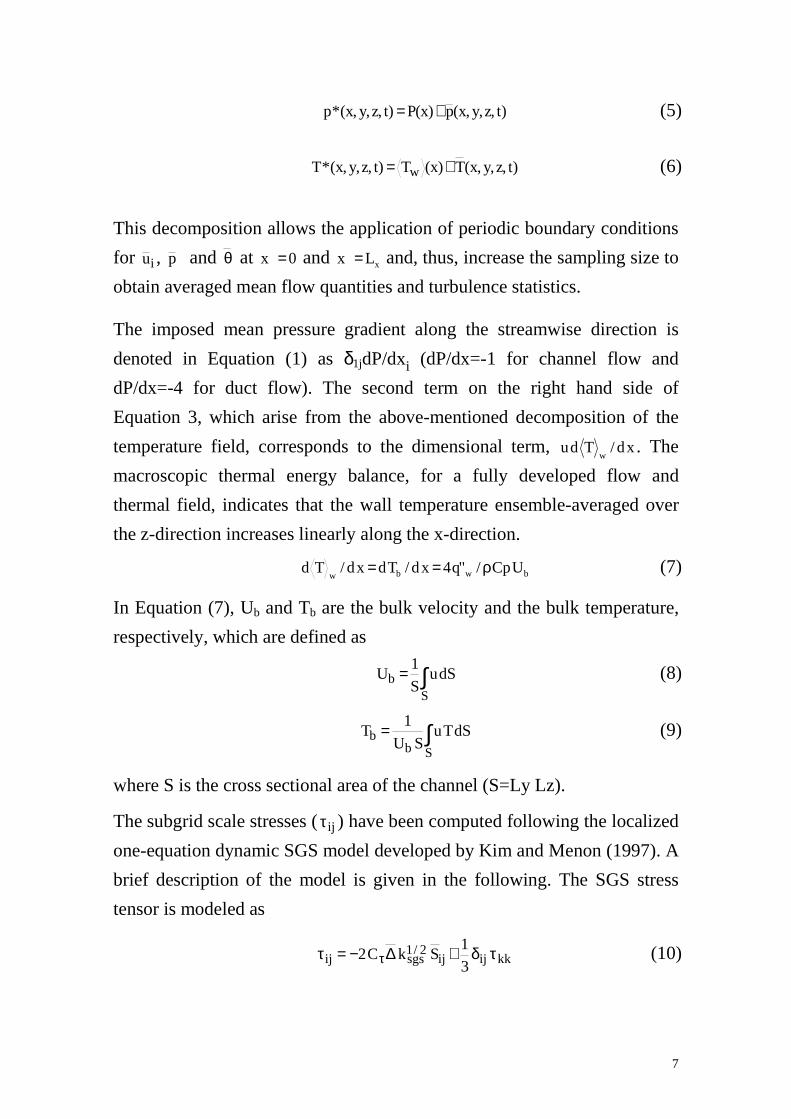
7
)t,z,y,x(p)x(P)t,z,y,x(*p += (5)
)t,z,y,x(T)x(T)t,z,y,x(*T w += (6)
This decomposition allows the application of periodic boundary conditions
for iu , p and θ at 0x = and xLx = and, thus, increase the sampling size to
obtain averaged mean flow quantities and turbulence statistics.
The imposed mean pressure gradient along the streamwise direction is
denoted in Equation (1) as δ1jdP/dxi (dP/dx=-1 for channel flow and
dP/dx=-4 for duct flow). The second term on the right hand side of
Equation 3, which arise from the above-mentioned decomposition of the
temperature field, corresponds to the dimensional term, xd/Tduw
. The
macroscopic thermal energy balance, for a fully developed flow and
thermal field, indicates that the wall temperature ensemble-averaged over
the z-direction increases linearly along the x-direction.
bwbwUCp/"q4xd/Tdxd/Td ρ== (7)
In Equation (7), Ub and Tb are the bulk velocity and the bulk temperature,
respectively, which are defined as
∫=S
b dSuS
1U (8)
∫=Sb
b dSTuSU
1T (9)
where S is the cross sectional area of the channel (S=Ly Lz).
The subgrid scale stresses ( ijτ ) have been computed following the localized
one-equation dynamic SGS model developed by Kim and Menon (1997). A
brief description of the model is given in the following. The SGS stress
tensor is modeled as
kkijij2/1
sgsij 3
1SkC2 τδ+∆−=τ τ (10)

8
where Cτ is a coefficient to be computed dynamically, ∆ is the
characteristic subgrid scale energy length (or grid scale), ksgs is the subgrid
scale kinetic energy and ijS is the resolved strain tensor. The second term
on the left-hand side of Equation (10) is included in the pressure term. The
subgrid scale kinetic energy (ksgs) is obtained by solving its transport
equation (see Kim and Menon, 1997), in which the dissipation term (εsgs) is
modeled as
∆=ε ε
2/3sgs
sgskC
(11)
where Cε is another coefficient also determined dynamically.
The procedure for computing the localized values of the model coefficients,
Cτ and Cε, is based, as in other localized dynamic SGS models (Piomelli,
1993) on the definition of a test scale field. The test filter, characterized by
∆ and equal to ∆2 , and applied to any variable φ , is denoted by φ . The
experimentally measured similarity (Liu et al. 1994) between the test scale
Leonard stresses, ( )jijiij uuuuL −= , and the SGS stresses allows a
reasonable assumption of the same parameterization for both tensors, τij
and Lij
kkijij2/1
testij L3
1SkˆC2L δ+∆−= τ (12)
where Lij is the resolved kinetic energy at the test scale. The over-
determined model coefficient Cτ in Equation (12) can be computed from
resolved quantities at the test filter level, using the least-square
minimization procedure.
ijij
ijij
SS
SL
2
1C =τ (13)
The dissipation rate of the test scale kinetic energy at the small scales is
produced by the molecular (ν) and the SGS viscosity (νSGS) and can be
written as

9
( )
∂∂
∂∂
−
∂∂
∂∂
ν+ν=εj
i
j
i
j
i
j
iSGStest x
u
x
u
x
u
x
u(14)
Similarity between the dissipation rates at the grid filter level (εsgs) and the
test filter level (εtest) is also invoked, and the dissipation model coefficient
(Cε) is computed as
2/3test
test
k
ˆC
ε∆=ε (15)
This model, based on the similarity between the SGS stress tensor and the
test scale Leonard stress tensor, overcomes the numerical stability
problems of the earlier dynamic models without any averaging or
adjustment of the model coefficients because the denominators of
Equations. (13) and (15) have well defined quantities. This is an important
feature when simulating turbulent flows under rotation because of the
stabilizing/destabilizing effects of rotation on turbulence. Kim and Menon
(1997) examined the properties of the model by conducting LES of
turbulent flows such as decaying, forced and rotating isotropic turbulence,
turbulent mixing layer and plane Couette flow. Their results showed good
agreement with existing experimental and DNS data.
As shown in Cabot and Moin (1993), who computed PrSGS=νSGS/αSGS from
DNS data of forced convection channel flow at Pr=0.7, PrSGS tends to reach
relatively constant values at large times and in the central region of the
channel (PrSGS≈0.4). Consequently, the SGS heat fluxes, hj, in Equation (3)
have been computed by assuming constant SGS Prandtl number (PrSGS
=0.4)
jSGS
SGSj xPr
h∂
θ∂ν−= (16)
The governing transport equations [Equations. (1 to 3)] were solved
numerically with the CALC-LES code (Davidson, 1997). This second-
order accuracy finite volume code uses central differencing of the diffusive
and convective terms on a collocated grid and a Crank-Nicolson scheme for

10
the temporal discretization. The coupling between the velocity and pressure
fields is solved efficiently by means of an implicit, two-step, time
advancement method and a multigrid solver for the resulting Poisson
equation (Emvin, 1997). This code has several optional SGS models
implemented and has been successfully tested in simulating various
transitional and turbulent flows of engineering interest such as flow around
obstacles (Krajnovic and Davidson, 1999; Sohankar et al. 1999 and
Sohankar, 2000) and buoyancy-driven and forced convection recirculating
flows in enclosures (Peng, 1997).
The computational domain was divided into 66x66x66 grid nodes for the
channel and duct flow simulations. They were uniformly distributed along
the homogeneous directions (∆x+ ≈37 and ∆z
+≈9 for the channel and
∆x+≈29 for the square duct) in which periodic boundary conditions were
imposed, while tanh distributions were used to stretch the nodes near the
walls where the no-slip condition was applied. For the Reynolds numbers
considered, the minimum and maximum grid spacing in the directions
perpendicular to the walls are (∆y+)min≈0.7 and (∆y
+)max≈11 for the
channel flow (Reτ=194) and (∆y+)min=(∆z
+)min≈0.4 and
(∆y+)max=(∆z
+)max≈9 for the square duct flow (Reτ=300). A constant wall
temperature, 0w =θ , was imposed at the four walls when simulating forced
convection channel flow.

11
3. RESULTS
Simulations of the isothermal stationary channel and duct flows started
from laminar velocity distributions at the final Reynolds numbers (Reτ=194
for channel flow and Reτ=300 for duct flow). With time, the flow
progressively and spontaneously became turbulent. The sampling
procedure used to obtain the average velocity fields and the turbulent
intensities was not started until the flow was statistically fully developed.
Results at the lowest rotation rate (Roτ=1.5) were obtained starting from an
instantaneous isothermal non-rotating flow field until a new statistically
steady state was reached. The rotation number was increased from 0 to 1.5
and from 1.5 to 3.6 maintaining a constant imposed pressure gradient (i.e.
constant value of Reτ). The computed mean wall stress (τw) is balanced by
the imposed pressure gradient within 0.05% in all the simulations reported
in this work. Instantaneous fully developed velocity and pressure fields of
channel flow were used as initial condition for the forced convection
simulation. The initial temperature field was computed from the
instantaneous streamwise velocity component using the analogy between
the momentum and heat transfer in the viscous sublayer (θ=Pr u). The bulk
velocity in Equation (3) was computed from the isothermal channel flow
simulations (Ub=15.9).
The sampling procedure used to obtain the average velocity fields and the
turbulent intensities and heat fluxes was not started until the flow and
thermal fields were statistically fully developed. The flow quantities were
averaged along the homogeneous directions as well as in time, typically
over about 15 and 40-70 non-dimensional time units for channel and duct
flows, respectively.
Table I summarizes the characteristics of rotating and non-rotating channel
and square duct flow studies used to validate the present simulations. In the
following discussion, the averaged resolved velocities, turbulent stresses

12
and turbulent heat fluxes are denoted as Ui, ’j
’iuu and ’’
iu θ , respectively,
for simplicity.Grid points Domain Reτ Roτ
Authorsx y z Lx Ly Lz (uτ D/ν) (2ΩD/uτ)
Kim et al. (1987)*1
192x129x160 4πx2x2π 180 0
Piomelli (1993) 48x65x64 4πx2xπ 200 0
Kristoffersen &
Andersson (1993)* 128x128x128 4πx2x2π 194 -7.5≤Roτ≤0
Alvelius (1999)* 384x129x240 8πx2x3π 180 0.1≤Roτ≤7.3
Isothermal channel flow
Present 66x66x66 4πx2xπ 194 0, 1.5, 3.6
Kasagi et al. (1992)1 128x97x128 5πx2x2π 150 0
Kawamura et al. (1999)2 128x66x128 3πx2x2π 180 0Forced convection
channel flow (Pr=0.71)
Present 66x66x66 4πx2xπ 194 0
Gavrilakis (1992)*1000x127x12
710πx1x1 300 0
Duct flow
Present 66x66x66 2πx1x1 300 0
Table I. Characteristics of direct* and large-eddy simulations.1Data available at: http://cfd.me.umist.ac.uk/ercofold/database/homepage.html2Data available at: http://muraibm.me.noda.sut.ac.jp/homepage/e-database1.html
Figures 2a and 2b show the streamwise mean velocity (U) profile along the
vertical direction and the computed turbulence intensities in the non-
rotating channel flow, respectively. It can be seen that the present results
are in good agreement with the DNS of Kim et al. (1987) and LES of
Piomelli (1993). The predicted non-dimensional centerline velocity is 18.2,
the same value reported by Kim et al. (1987) and the dimensionless bulk
velocity (Ub=15.9, Re=2ReτUb=6170) is 1.7% higher than the DNS results.
The computed friction factor (f= 2τw/ρ =0.0078) is within 5% of the
correlation of experimental data (Dean, 1978).

13
y+
U
100
100
101
101
102
102
0 0
5 5
10 10
15 15
20 20(a)
Law of the wallDNS. Kim et al. (1987)LES. Piomelli (1993)LES. Present
y+
u rms,
v rms,
wrm
s
0
0
50
50
100
100
150
150
200
200
0 0
0.5 0.5
1 1
1.5 1.5
2 2
2.5 2.5
3 3(b)
urms
vrms
wrms
Lines: DNS. Kim et al. (1987)Filled symbols: LES. Piomelli (1993)Open symbols: Present
Figure 2. Averaged velocity (a) and turbulence intensities (b) profiles in non-rotating channel flow.
The results of Piomelli (1993) were obtained using the dynamic SGS model
of Germano et al. (1991) to compute the model coefficient. This procedure
assumes the model coefficient to be a function only of time and
inhomogeneous directions, C(y,t). It can be seen that the urms values in the
logarithmic layer are better reproduced by the present predictions. This
may be attributed to the slightly higher grid resolution in the streamwise
direction of the present simulations (see Table I). However, the fact that the
LES of Piomelli (1993) were conducted with a higher accuracy code seems
to indicate that the difference may be connected with a better performance
of the Kim and Menon (1997) SGS model.

14
y
U
-1
-1
-0.75
-0.75
-0.5
-0.5
-0.25
-0.25
0
0
0.25
0.25
0.5
0.5
0.75
0.75
1
1
0 0
5 5
10 10
15 15
20 20
25 25(a)DNS. Reτ=180, Roτ=1.8. Alvelius (1999)LES. Reτ=194, Roτ=1.5. Present
y
U
-1
-1
-0.75
-0.75
-0.5
-0.5
-0.25
-0.25
0
0
0.25
0.25
0.5
0.5
0.75
0.75
1
1
0 0
5 5
10 10
15 15
20 20
25 25(b)DNS. Reτ=180. Roτ=3.6. Alvelius (1999)LES. Re’t=194. Roτ=3.6. Present
y
u rms,
v rms,
wrm
s
-1
-1
-0.5
-0.5
0
0
0.5
0.5
1
1
0 0
0.5 0.5
1 1
1.5 1.5
2 2
2.5 2.5
3 3
3.5 3.5(c)
Lines: DNS. Reτ=180, Roτ=1.8. Alvelius (1999)Symbols: LES. Reτ=194, Roτ=1.5. Presenturms
wrms
vrms
y
u rms,
v rms,
wrm
s
-1
-1
-0.5
-0.5
0
0
0.5
0.5
1
1
0 0
0.5 0.5
1 1
1.5 1.5
2 2
2.5 2.5
3 3
3.5 3.5(d)
vrms
urms
wrms
Lines: DNS. Reτ=180, Roτ=3.6. Alvelius (1999)Symbols: LES. Reτ=194, Roτ=3.6. Present
Figure 3. Averaged velocity (a and b) and turbulence intensities (c and d) inrotating channel flow.

15
Figures 3a and 3b show the mean streamwise velocity and turbulence
intensities’ vertical profiles of rotating channel flow at Roτ=1.5,
respectively. The DNS of Alvelius (1999) at Roτ=1.8 and Roτ=3.6 were
selected for the comparison because the computational domain used by this
author is the largest of the rotating channel flow studies shown in Table I
and has the same grid resolution as the DNS of Kim et al. (1987). Good
agreement is found when comparing, in Figure. 3, the DNS of Alvelius
(1999) and the present results. As shown in Figures 3a and 3b, the average
velocity profile becomes asymmetric as the rotation number is increased. It
can be seen in Figures 3a and 3b that the present predictions accurately
reproduce the quasi-linear region of the profile U(y), where the absolute
mean vorticity, -(dU/dy)+Roτ becomes approximately zero (see
Kristoffersen and Andersson, 1993)
Figures 3b and 3d show that Reynolds stresses are generally reduced in
comparison with the non-rotating case (Figure 2b) on the stable side (near
the stable wall, y=1) and that they are generally increased on the unstable
side (near the unstable wall, y=-1). Detailed analyses of the effects of
rotation on the different Reynolds stresses based on the generation terms of
the transport equations, are reported in Johnston et al. (1972) and
Kristoffersen and Andersson (1993).
Comparison of averaged temperatures and heat fluxes in forced convection
flow at Reτ=194 (Re=6170) and Pr=0.7 are shown in Figure 4. It can be
seen that a good agreement is found comparing the present LES obtained
with a constant PrSGS number and DNS data of Kasagi et al. (1992) and
Kawamura et al. (1998). The value of the Nusselt number (Nu=20.7) is a
5% larger than the one predicted by the Gnielisky’s correlation (Gnieliski,
1976).

16
y+
Θ+
10-1
10-1
100
100
101
101
102
102
0 0
2 2
4 4
6 6
8 8
10 10
12 12
14 14
16 16Law of the wall
DNS, Reτ=150, Kasagi et al. (1992)
DNS, Reτ=180, Kawamura et al. (1998)
LES, Reτ=194, Present
(a)
y+
⟨θ’2 ⟩,
⟨u’θ
’⟩,-
⟨v’θ
’⟩
0
0
50
50
100
100
150
150
200
200
0 0
1 1
2 2
3 3
4 4
5 5
6 6
7 7
Lines: DNS, Reτ=150, Kasagi et al. (1992)
Open symbols: DNS, Reτ=180, Kawamura et al. (1998)
Solid symbols: LES, Reτ=194, Present
⟨u’θ’⟩⟨θ’2⟩
- ⟨v’θ’⟩
(b)
Figure 4. Averaged temperature (a) and turbulent heat fluxes (b) profiles in non-rotating channel flow
Turbulent flow in a non-rotating square duct was simulated at Reτ=300 and
the results compared with DNS of Gavrilakis (1992) at the same value of
Reτ and experiments of Cheesewright et al. (1990) at Rec=4900, based on
the centerline velocity, which is close to the value in the present
computation (Rec=5900).

17
181610
18
16
10
z
y
0
0
0.1
0.1
0.2
0.2
0.3
0.3
0.4
0.4
0.5
0.5
0 0
0.1 0.1
0.2 0.2
0.3 0.3
0.4 0.4
0.5 0.5
1
Figure 5. Averaged flow field in a non-rotating square duct in terms of contours ofthe streamwise velocity component and cross-stream vector field. The vector nearthe bottom right corner has a length of 1.
y
u rms,
v rms,
wrm
s
0 0.25 0.5 0.75 10
0.5
1
1.5
2
2.5
3
3.5
urms
wrms
vrms
Lines: DNS. Gavrilakis (1992)Symbols: LES. Present
Figure 6. Averaged turbulent intensity profiles along the wall bisector (z=0.5) innon-rotating duct flow at Reτ=300.
18
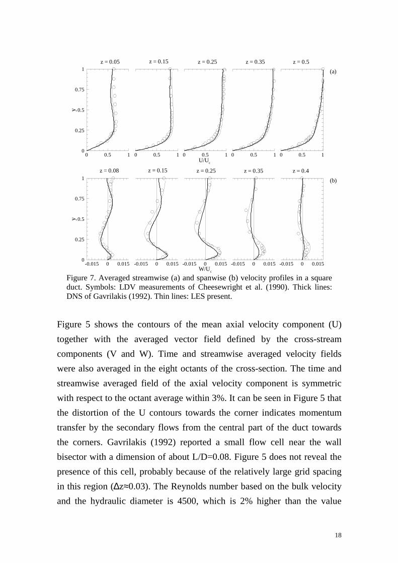
Figure 7. Averaged streamwise (a) and spanwise (b) velocity profiles in a squareduct. Symbols: LDV measurements of Cheesewright et al. (1990). Thick lines:DNS of Gavrilakis (1992). Thin lines: LES present.
Figure 5 shows the contours of the mean axial velocity component (U)
together with the averaged vector field defined by the cross-stream
components (V and W). Time and streamwise averaged velocity fields
were also averaged in the eight octants of the cross-section. The time and
streamwise averaged field of the axial velocity component is symmetric
with respect to the octant average within 3%. It can be seen in Figure 5 that
the distortion of the U contours towards the corner indicates momentum
transfer by the secondary flows from the central part of the duct towards
the corners. Gavrilakis (1992) reported a small flow cell near the wall
bisector with a dimension of about L/D=0.08. Figure 5 does not reveal the
presence of this cell, probably because of the relatively large grid spacing
in this region (∆z≈0.03). The Reynolds number based on the bulk velocity
and the hydraulic diameter is 4500, which is 2% higher than the value
y
-0.015 0 0.0150
0.25
0.5
0.75
1
z = 0.08
y
0 0.5 10
0.25
0.5
0.75
1z = 0.05
0 0.5 1U/Uc
z = 0.25
0 0.5 1
z = 0.15
-0.015 0 0.015
z = 0.15
-0.015 0 0.015W/Uc
z = 0.25
0 0.5 1
z = 0.35
-0.015 0 0.015
z = 0.35
0 0.5 1
z = 0.5
(a)
-0.015 0 0.015
z = 0.4
(b)

19
calculated by Gavrilakis (1992). The predicted friction factor (f=0.0093) is
the same as that obtained with Dean’s correlation for ducts (Dean, 1978).
The volume averaged turbulent kinetic energy, 2.14, agrees well with that
reported by Gavrilakis (1992), 2.1. Figure 6 shows the profiles of the
normal turbulent stresses along the wall bisector (z=0.5). The maximum
value of the averaged secondary velocities (≈0.3) is well below the
magnitude of the rms values shown in Figure 6. Figures 7a and 7b show the
vertical profiles of the axial and cross-stream velocities at different
horizontal positions. The centerline velocity (Uc) was adopted as the
velocity scale in these figures because it is the only one available in the
experiments of Cheesewright et al. (1990). Good agreement is found when
comparing present predictions of the velocity fields (Figures 7a and 7b) and
the turbulence statistics (Figure 6) along the wall bisector with DNS and
experiments.
4. CONCLUSIONS
Fully developed turbulent flows at low Reynolds numbers in stationary and
rotating channels as well as in a non-rotating square duct have been
simulated using a second order code with a one-equation dynamic subgrid
scale model. Present predictions of the averaged velocity and turbulent
stresses are in good agreement with existing direct numerical simulations.
Large-eddy simulations of turbulent forced convection flows in a stationary
channel have been also conducted. It has been found that the assumption of
constant subgrid scale Prandlt number reproduces accurately the averaged
temperature and turbulent heat fluxes of available direct numerical
simulations.

20
AKNOWLEDGMENTS
This work was conducted during the first author stay at the Department of
Thermo and Fluid Dynamics (Chalmers University of Technology). The
support of SEUID (Ministry of Education and Technology of Spain) is
gratefully aknowledged. We would like to thank S. Gavrilakis, K. Alvelius
and A. Johansson for providing us the data from their simulations.
REFERENCES
Alvelius K. (1999) Studies of turbulence and its modeling through large
eddy- and direct numerical simulation PhD thesis, Dept. of Mechanics,
Royal Institute of Technology, Stockholm
Cabot W. and Moin P. "Large eddy simulations of scalar transport with the
dynamic subgrid-scale model" in Large eddy simulation of complex
engineering and geophysical flows. B. Galperin and S. A. Orszag, editors.
Cambridge University Press, 1993
Cheesewright R., McGrath G. and Petty D. G. (1990) LDA measurements
of turbulent flow in a duct of square cross section at low Reynolds number
Aeronautical Engineering Dept. Rep. ER 1011. Queen Mary Westfield
College. University of London.
Davidson L. (1997) LES of recirculating flow without any homogeneous
direction: A dynamic one-equation subgrid model, in 2nd Int. Symp. on
Turbulence Heat and Mass Transfer, Delft, Delft University Press. pp 481-
490
Dean R. B. (1978) Reynolds number dependence of skin friction and other
bulk flow variables in two-dimensional rectangular duct flow J. Fluids
Eng. 100, 215

21
Emvin P. (1997) The full multigrid method applied to turbulent flow in
ventilated enclosures using structured and unstructured grids, PhD thesis,
Dept. of Thermo and Fluid Dynamics, Chalmers University of Technology,
Gothenburg
Gavrilakis S. (1992) Numerical simulations of low-Reynolds-number
turbulent flow through a straight square duct J. Fluid Mech. 244, 101
Germano M., Piomelli U., Moin P. and Cabot W. H. (1991) A dynamic
subgrid-scale eddy viscosity model," Phys. Fluids A 3, 1760
Gnielisky V. (1976) New equations for heat and mass transfer in turbulent
pipe and channel flow, Int. Chem. Eng. 16, 359.
Huser A. and Biringen S. (1993) Direct numerical simulation of turbulent
flow in a square duct J. Fluid Mech. 257, 65
Johnston J. P., Hallen R. M. and Lezius D. K. (1972) Effects of spanwise
rotation on the structure of two-dimensional fully developed turbulent
channel flow J. Fluid Mech. 56, 533
Kasagi N., Tomita Y. and Kuroda A. (1992) Direct numerical simulation of
passive scalar field in a turbulent channel flow J. Heat Transfer 114, 598
Kawamura H., Abe H. and Matsuo Y. (1999) DNS of turbulent heat
transfer in channel flow with respect to Reynolds and Prandtl number effect
Int. J. Heat and Fluid Flow 20, 196.
Kim J., Moin P. and Moser R. (1987) Turbulence statistics in fully
developed channel flow at low Reynolds number J. Fluid Mech. 177, 133
Kim W. and Menon S. (1997) Application of the localized dynamic
subgrid-scale model to turbulent wall-bounded flows, AIAA Paper 97-
0210. 35th Aerospace Sciences Meeting & Exhibit, Reno, NV
22
Krajnovic S. and Davidson L. (1999) Large-eddy simulation of the flow
around a surface-mounted cube using a dynamic one-equation subgrid
model, 1st Int. Symp. on Turbulence and Shear Flow Phenomena, Santa
Barbara.
Kristoffersen R. and Andersson H. (1993) Direct simulations of low-
Reynolds-number turbulent flow in a rotating channel J. Fluid Mech. 256,
163
Lamballais E., Lesieur M. and Métais O. (1996) Effects of spanwise
rotation on the vorticity stretching in transitional and turbulent channel
flow Int. J. Heat and Fluid Flow, 17, 324
Liu S., Meneveau C. and Katz J. (1994) On the properties of similarity
subgrid-scale models as deduced from measurements in a turbulent jet J.
Fluid Mech. 275, 83
Madabhushi R. V. and Vanka S. P. (1991) Large-eddy simulation of
turbulence-driven secondary flows in a square duct Phys. Fluids A 3, 2734
Miyake Y. and Kajishima T. (1986) Numerical simulation of the effect of
Coriolis force on the structure of turbulence Bulletin of JSME. 29, 3341
Peng S. (1997) Modelling of turbulent flow and heat transfer for building
ventilation, PhD thesis, Dept. of Thermo and Fluid Dynamics, Chalmers
University of Technology, Gothenburg.
Piomelli U. (1993) High Reynolds number calculations using the dynamic
subgrid-scale stress model Phys. Fluids A 5, 1484
Piomelli U. and Liu J. (1995) Large-eddy simulation of rotating channel
flows using a localized dynamic model," Phys. Fluids A 7, 839

23
Sohankar A., Davidson L. and Norberg C. (2000) Large eddy simulation of
flow past a square cylinder: Comparison of different subgrid scale models,
J. Fluids Eng. 122, 39. See also Erratum, J. Fluids Eng. 122, 643
Sohankar A., Norberg C. and Davidson L. (1999) Simulation of three-
dimensional flow around a square cylinder at moderate Reynolds numbers
Phys. Fluids A 11, 288
Tafti D. K. and Vanka S. P. (1991) A numerical study of the effects of
spanwise rotation on turbulent channel flow Phys. Fluids A 3, 642