Embed Size (px)
Citation preview

Chalmers Publication Library
Copyright Notice
©2012 IEEE. Personal use of this material is permitted. However, permission to
reprint/republish this material for advertising or promotional purposes or for creating new
collective works for resale or redistribution to servers or lists, or to reuse any copyrighted
component of this work in other works must be obtained from the IEEE.
This document was downloaded from Chalmers Publication Library (http://publications.lib.chalmers.se/),
where it is available in accordance with the IEEE PSPB Operations Manual, amended 19 Nov. 2010, Sec.
8.1.9 (http://www.ieee.org/documents/opsmanual.pdf)
(Article begins on next page)

1
Cooperative Received Signal Strength-Based
Sensor Localization with Unknown Transmit
PowersReza Monir Vaghefi,Student Member, IEEE,Mohammad Reza Gholami,Student
Member, IEEE,
R. Michael Buehrer,Senior Member, IEEE,and Erik G. Strom,Senior Member, IEEE,
Abstract
Cooperative localization (also known as sensor network localization) using received signal strength
(RSS) measurements when the source transmit powers are different and unknown is investigated. Previous
studies were based on the assumption that the transmit powers of source nodes are the same and perfectly
known which is not practical. In this paper, the source transmit powers are considered as nuisance
parameters and estimated along with the source locations. The corresponding Cramer-Rao lower bound
(CRLB) of the problem is derived. To find the maximum likelihood (ML) estimator, it is necessary to
solve a nonlinear and nonconvex optimization problem, which is computationally complex. To avoid the
difficulty in solving the ML estimator, we derive a novel semidefinite programming (SDP) relaxation
technique by converting the ML minimization problem into a convex problem which can be solved
efficiently. The algorithm requires only an estimate of the path loss exponent (PLE). We initially assume
that perfect knowledge of the PLE is available, but we then examine the effect of imperfect knowledge
of the PLE on the proposed SDP algorithm. The complexity analyses of the proposed algorithms are
also studied in detail. Computer simulations showing the remarkable performance of the proposed SDP
algorithm are presented.
Copyright (c) 2012 IEEE. Personal use of this material is permitted. However, permission to use this material for any otherpurposes must be obtained from the IEEE by sending a request to [email protected].
R. M. Vaghefi and R. M. Buehrer are with the Mobile and PortableRadio Research Group, Bradley Department of Electricaland Computer Engineering, Virginia Polytechnic Instituteand State University (Virginia Tech), Blacksburg, VA 24061USA(e-mail: [email protected]; [email protected])
M. R. Gholami and E. G. Strom are with the Division of Communication Systems and Information Theory, Departmentof Signals and Systems, Chalmers University of Technology,SE-412 96 Gothenburg, Sweden (e-mail: [email protected];[email protected]).
This work was supported in part by the Swedish Research Council (contract no. 2007-6363). This paper was presented inpart at the IEEE International Conference on Acoustics, Speech and Signal Processing (ICASSP), Prague, Czech Republic, May22-27, 2011.
October 25, 2012 DRAFT

2
Index Terms
Received Signal Strength (RSS), cooperative sensor localization, transmit power, maximum like-
lihood (ML), semidefinite programming (SDP), linear least squares (LLS), path loss exponent (PLE),
computational complexity.
I. INTRODUCTION
Recently, wireless sensor networks (WSN) have been the subject of great interest in many studies
because of their wide applications in control, tracking, and monitoring. Location information is a vital
aspect of many WSNs. Indeed, the location of each sensor is often required to make the collected
information useful. Generally, in a WSN, the positions of a number of sensors are known (anchor nodes),
while there are some sensors (source nodes) whose positionsare unknown and thus must be estimated
using sensor localization. The main purpose of sensor localization is to determine the location of sensors
in a WSN via noisy measurements [1]. These measurements may include received signal strength (RSS)
[2]–[4], time-of-arrival [5], [6], time-difference-of-arrival [7]–[9], and angle-of-arrival [10], [11]. Among
the different types of measurements, RSS is a popular methodmainly because of its low complexity and
cost in software and hardware implementations [1].
Sensor localization is generally divided into two cases: non-cooperative and cooperative. In the non-
cooperative case, source nodes can communicate only with anchor nodes [1], [12]. The lack of accessible
anchor nodes and also limited connectivity among anchor nodes and source nodes have led to the
emergence of cooperative localization in which source nodes are able to communicate with both anchor
nodes and other source nodes. Therefore, not only are the RSSvalues between source nodes and anchor
nodes (source-anchor measurements) measured, but also thesource nodes themselves are involved and
collect RSS measurements from each other (source-source measurements). Furthermore, in cooperative
localization, anchor nodes can estimate the location of allsource nodes simultaneously. Thus, both
estimation performance and robustness are improved by employing cooperative localization [1], [3],
[13].
The maximum likelihood (ML) estimator and the Cramer-Rao lower bound (CRLB) of cooperative RSS
localization were studied in [1]. The cost function of the MLestimator is severely nonlinear and noncovex
and, therefore, it can be optimized by iterative algorithmsonly with an appropriate initialization [14], [15].
October 25, 2012 DRAFT

3
The performance of iterative algorithms strongly depends on the initial solution. If the initialization is not
sufficiently close to the global minimum, the iterative algorithm may converge to a local minimum or a
saddle point causing a large estimation error. Therefore, determining an appropriate initialization point is
a crucial problem in optimizing the ML cost function. As a result, some approaches such as grid search
methods, linear estimators, and convex relaxation techniques have been introduced to address the ML
problem [3], [12], [16]. The grid search methods are not generally popular because they are very time-
consuming and require a huge amount of memory when the numberof the unknown parameters is too
large. Linear estimators having a closed-form solution areusually derived based on many approximations
[12], [17]–[19] which affect its performance, especially when shadowing is very high [19]. A convex
relaxation technique such as semidefinite programming (SDP) is another solution for the ML convergence
problem [13], [16], [19]–[24]. In the semidefinite relaxation technique, the nonlinear and nonconvex ML
problem is transformed into a convex optimization problem.The advantage of an SDP is that its cost
function does not have local minima and thus convergence to the global minimum is guaranteed [25], [26].
The downside is that the SDP technique is sub-optimal and cannot achieve the best possible performance
in all conditions. Most studies mentioned above on RSS localization assume that the source transmit
powers are the same and known [4], [13], [17], [23].
The RSS measurement model depends on the transmit power of the source nodes. Therefore, the anchor
nodes are not able to find the location of a source node if its transmit power is not accounted for. Each
source node has a specific transmit power depending on, e.g.,its battery and antenna gain. In addition,
the transmit power might change with time, e.g., when batteries begin to exhaust. Consequently, each
source node has to report its transmit power to anchor nodes constantly during RSS measurements which
requires additional hardware and software in both anchor nodes and source nodes making the network
more convoluted [1]. When the transmit powers are not available, there are generally two common
solutions suggested to address this problem. First, one canestimate the transmit power of the source
along with its location [19], [27]. Second, one can eliminate the dependency of the transmit power from
the RSS measurement model by using the differential RSS between a source node and two anchor nodes
[19], [28], [29]. The number of unknown parameters in the latter method is fewer than in the former
method. However, employing the latter method introduces noise correlation and noise enhancement which
complicate the computations and degrade the accuracy [19].It should also be noted that all previous
October 25, 2012 DRAFT

4
studies on RSS localization with unknown transmit power arefor the non-cooperative case. In this paper,
for the first time, we examine this problem for the cooperative localization case. Some range-free and
non-model-based techniques were also suggested [30], [31]in which the localization algorithms do not
require the model parameters, such as the transmit power andthe path loss exponent, and the estimate of
the source location was basically obtained based on the comparisons among RSS measurements. However,
having a cooperative network and source nodes with different transmit powers make those algorithms
complex and inapplicable.
Thus, cooperative localization using RSS in the practical case where transmit powers are different and
unknown is currently an open problem. In this paper, we consider this problem and provide a solution.
Specifically, the source transmit powers are considered as nuisance parameters and estimated jointly with
the source node locations. A novel SDP technique is introduced for this expanded estimation problem.
To make the derivations easier to understand, we start by describing the proposed SDP algorithm for
the non-cooperative case. Then, the measurement model is extended to the cooperative case and the
corresponding SDP algorithm is derived. The original ML estimator is transformed into an approximate
nonlinear least squares (NLS) problem. Then, an appropriate relaxation is applied to convert the NLS
problem into an SDP optimization problem. It is worth mentioning that the SDP techniques introduced
in [16], [20] are not applicable here, since they assumed that noisy pairwise distances between source
nodes and anchor nodes are available. However, in our study,the distances cannot be computed because
the transmit powers of the source nodes are not available to the estimator. Ouyang et al. [13] also derived
an SDP approach which is directly applied to the RSS model. However, they assumed that all source
nodes have the same known transmit power which is not practical. Conversely, in the current work, we
assume that each source node has a unique transmit power which is not known. The Cramer-Rao lower
bound (CRLB) of this problem is computed. We also propose a linear estimator for comparison with the
proposed SDP algorithm. Moreover, we investigate the effect of imperfect knowledge of the path loss
exponent (PLE) on the algorithms’ accuracy and introduce a novel technique to improve performance
when the PLE is estimated. We also study the computational complexity of the considered algorithms in
detail.
The rest of the paper is organized as follows. Section II presents the non-cooperative RSS localization
problem, introducing the measurement model and proposed localization algorithms. The extension of RSS
October 25, 2012 DRAFT

5
localization to the cooperative case is discussed in Section III. Section IV describes the effect of imperfect
knowledge of the PLE on the proposed algorithms. Complexityanalyses of the proposed algorithms are
given in Section V. The simulation results and algorithm comparisons are discussed in Section VI. Finally,
Section VII concludes the paper. In Appendix A, the corresponding CRLB of the measurement model
is derived. The proposed linear estimator is derived in Appendix B. The full details of the complexity
analyses are given in Appendix C.
Notation. Throughout the paper, the following notations are used. Lowercase and uppercase symbols
denote scalar values. Bold uppercase symbols and bold lowercase symbols denote matrices and vectors,
respectively.‖ · ‖ denotesℓ2 norm. diag {·} represents a diagonal matrix.|A| represents the cardinality
(number of elements) of the setA. IM and 0M denote theM by M identity and theM by M zero
matrices, respectively. For arbitrary symmetric matricesA andB, A � B means thatA−B is positive
semidefinite.[a]i and [A]i,j denote theith element of vectora and the element at theith row andjth
column of matrixA, respectively.[A;B] means that matricesA andB are concatenated vertically.
II. N ON-COOPERATIVE LOCALIZATION
This section describes the RSS localization model for the non-cooperative case. In non-cooperative
localization problems, only the measurements between a source node and the anchor nodes are considered
and the location of each source node is estimated independently. A network in a two-dimensional space
is considered1. Let x = [a, b]T ∈ R2 be the unknown coordinates of the source node to be determined.
Denote byC = {1, . . . ,M} the set of indices of the anchor nodes, byyi = [xi, yi]T ∈ R
2, i ∈ C, the
known location of the anchor nodes. LetA = { i | i ∈ C,anchor nodei is connected to source node}
be the set of the indices of the anchor nodes connected to the source node. The received power (in dBm)
at theith anchor node,Pi, under log-normal shadowing is modeled as [2]
Pi = P0 − 10β log10did0
+ ni, i ∈ A, (1)
whereP0 (in dBm) is the reference power at distanced0 from the source (which depends on the transmit
power),β is the path loss exponent,di = ‖yi − x‖ is the true distance between the source node and
the ith anchor node, andni are the log-normal shadowing terms modeled as independent and identically
1The generalization to a three-dimensional space is straightforward, but is not explored in this paper.
October 25, 2012 DRAFT
6
distributed (i.i.d.) zero-mean Gaussian random variableswith standard deviationσdB for i ∈ A. The
variance of the shadowing term is constant with distance andonly depends on the environment where the
network is set up [1]. Without loss of generality, we assumed0 = 1 m. In this case, there are 3 unknown
parameters that should be estimated including the source node coordinates and its transmit power.
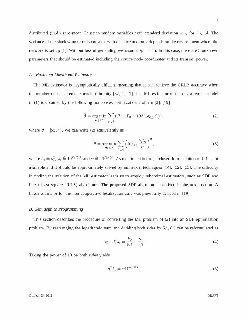
A. Maximum Likelihood Estimator
The ML estimator is asymptotically efficient meaning that itcan achieve the CRLB accuracy when
the number of measurements tends to infinity [32, Ch. 7]. The ML estimator of the measurement model
in (1) is obtained by the following nonconvex optimization problem [2], [19]
θ = argminθ∈R3
∑
i∈A
(Pi − P0 + 10β log10 di)2 , (2)
whereθ = [x;P0]. We can write (2) equivalently as
θ = argminθ∈R3
∑
i∈A
(
log10hiλi
α
)2
, (3)
wherehi , d2i , λi , 10Pi/5β , andα , 10P0/5β . As mentioned before, a closed-form solution of (2) is not
available and it should be approximately solved by numerical techniques [14], [32], [33]. The difficulty
in finding the solution of the ML estimator leads us to employ suboptimal estimators, such as SDP and
linear least squares (LLS) algorithms. The proposed SDP algorithm is derived in the next section. A
linear estimator for the non-cooperative localization case was previously derived in [19].
B. Semidefinite Programming
This section describes the procedure of converting the ML problem of (2) into an SDP optimization
problem. By rearranging the logarithmic term and dividing both sides by5β, (1) can be reformulated as
log10 d2i λi =
P0
5β+
ni
5β. (4)
Taking the power of 10 on both sides yields
d2iλi = α10ni/5β . (5)
October 25, 2012 DRAFT

7
For sufficiently small noise, the right-hand side (RHS) of (5) can be approximated using the first-order
Taylor series expansion as
d2iλi = α
(
1 +ln 10
5βni
)
. (6)
This can be rewritten as
d2i λi = α+ ǫi, (7)
whereǫi is a zero-mean Gaussian random variable with variance(ln10)2α2σ2dB/25β
2. The corresponding
NLS estimator of the unknown parameters[x; α] in (7) is [32, Ch. 8]
[x; α] = argmin[x;α]∈R3
∑
i∈A
(hiλi − α)2 . (8)
The cost function (8) is still nonlinear and noncovex. In thenext step, an auxiliary variablez is defined
as
z = xTx. (9)
The minimization problem of (8) can be relaxed to an SDP optimization problem as [25]
minimizex,z,α,hi
∑
i∈A
(hiλi − α)2 (10a)
subject to hi =
yi
−1
T
I2 x
xT z
yi
−1
, (10b)
I2 x
xT z
� 03. (10c)
The solution of (10) can be effectively found with well knownalgorithms such as interior point methods
[25], [26]. In MATLAB simulations, standard SDP solvers such as SeDuMi or SDPT3 [34], [35] are
employed to solve SDP optimization problems. Note that we have employed the inequality constraint
(10c) instead of the equality in (9) to relax the cost function in (8) to a convex problem in (10) [16],
[20], [25].
In summary, an SDP solution for RSS localization with unknown transmit power is introduced by
converting the nonconvex cost function of the ML estimator into a convex cost function using two steps
of approximations and relaxations. In the first step, the ML cost function in (3) is approximated by
October 25, 2012 DRAFT

8
0
0.5
1
1.5
2
00.5
11.5
2
0
1
2
3
4
hα
(λh− α)2 log210(λh/α)
(a)
0
5
10
15
20
0
5
10
15
200
1000
2000
3000
4000
5000
ab
(b)
0
5
10
15
20
0
5
10
15
200
800
1600
2400
3200
4000
ab
(c)
Fig. 1. (a) illustration of functions(λh−α)2 and log210(λh/α) versus unknown variablesh andα (for simplicity, λ = 1), (b)
cost function of (3), (c) cost function of (8) versusa andb coordinates (source location), the minimum of the cost functions isindicated by a white square.
another cost function of (8). More specifically, the function∑
i(λihi−α)2 is substituted for the function∑
i log210(λihi/α). Fig. 1 depicts the two mentioned functions versus unknown parametersh andα (λ
is a known parameter). As can be seen, these functions have similar behaviors; the minimum of both
functions appears atλh = α and both monotonically increase and decrease in the same regions. Note that
the valueλ changes the minimum of the functions but does not affect their general behaviors. Hence, for
simplicity λ = 1 has been selected for the illustration. Fig. 1 also depicts one realization of the ML cost
function of (3) and the cost function of (8). A source is located at [10, 10]T and five anchor nodes are
randomly placed inside a square area 20 m× 20 m. The standard deviation of log-normal shadowing is
3 dB and the path loss exponent is set to 4. Since it is not possible to show a plot in four-dimensional
space, the value ofP0 is fixed at the true value (-10 dBm) and the functions are plotted versusa and
b coordinates. Fig. 1b shows the cost function of the ML estimator given in (3) which has a global
minimum at [10.5, 11.5]T (the step of the mesh grid is 0.5) and some local minima and saddle points,
e.g., a local minimum at[2.5, 17.5]T . The cost function of (8), shown in Fig. 1c, is much smoother
than (3) and has a global minimum at[10, 11.5]T . However, it has some concave areas around its global
minimum. It, therefore, still must be relaxed to a convex shape. In the next step, by using the relaxation
of (10c), the function in (8) is relaxed to a convex function in (10). The solution of (8) and (10) for the
source location will coincide if the minimum of (10) occurs for x andz such thatz = xTx.
October 25, 2012 DRAFT
9
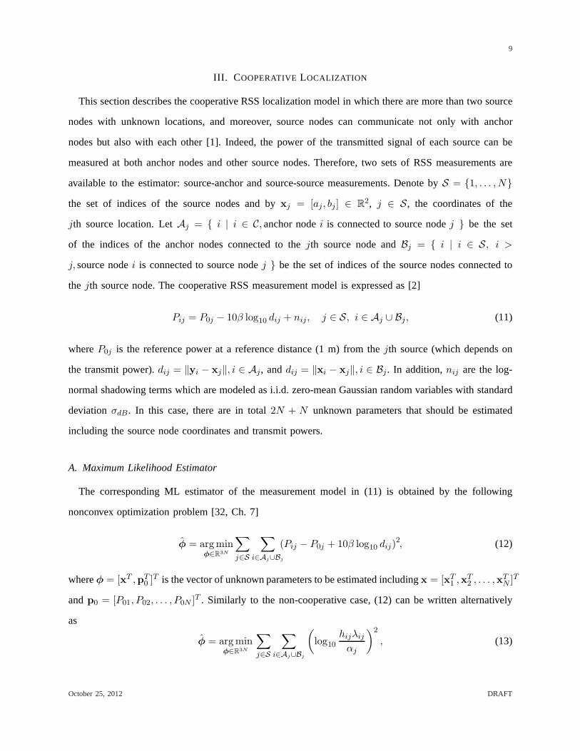
III. C OOPERATIVE LOCALIZATION
This section describes the cooperative RSS localization model in which there are more than two source
nodes with unknown locations, and moreover, source nodes can communicate not only with anchor
nodes but also with each other [1]. Indeed, the power of the transmitted signal of each source can be
measured at both anchor nodes and other source nodes. Therefore, two sets of RSS measurements are
available to the estimator: source-anchor and source-source measurements. Denote byS = {1, . . . , N}
the set of indices of the source nodes and byxj = [aj, bj ] ∈ R2, j ∈ S, the coordinates of the
jth source location. LetAj = { i | i ∈ C,anchor nodei is connected to source nodej } be the set
of the indices of the anchor nodes connected to thejth source node andBj = { i | i ∈ S, i >
j, source nodei is connected to source nodej } be the set of indices of the source nodes connected to
the jth source node. The cooperative RSS measurement model is expressed as [2]
Pij = P0j − 10β log10 dij + nij, j ∈ S, i ∈ Aj ∪ Bj, (11)
whereP0j is the reference power at a reference distance (1 m) from thejth source (which depends on
the transmit power).dij = ‖yi − xj‖, i ∈ Aj, anddij = ‖xi − xj‖, i ∈ Bj. In addition,nij are the log-
normal shadowing terms which are modeled as i.i.d. zero-mean Gaussian random variables with standard
deviationσdB . In this case, there are in total2N + N unknown parameters that should be estimated
including the source node coordinates and transmit powers.
A. Maximum Likelihood Estimator
The corresponding ML estimator of the measurement model in (11) is obtained by the following
nonconvex optimization problem [32, Ch. 7]
φ = argminφ∈R3N
∑
j∈S
∑
i∈Aj∪Bj
(Pij − P0j + 10β log10 dij)2, (12)
whereφ = [xT ,pT0 ]
T is the vector of unknown parameters to be estimated includingx = [xT1 ,x
T2 , . . . ,x
TN ]T
andp0 = [P01, P02, . . . , P0N ]T . Similarly to the non-cooperative case, (12) can be writtenalternatively
as
φ = argminφ∈R3N
∑
j∈S
∑
i∈Aj∪Bj
(
log10hijλij
αj
)2
, (13)
October 25, 2012 DRAFT
10
wherehij , d2ij , λij , 10Pij/5β , andαj , 10P0j/5β . The proposed SDP algorithm is derived in the next
section. We also formulate the proposed LLS algorithm for cooperative localization in Appendix B.
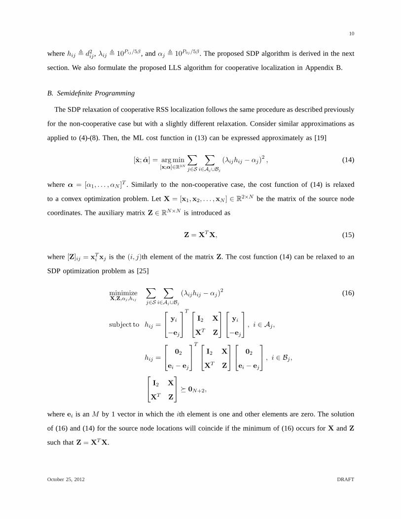
B. Semidefinite Programming
The SDP relaxation of cooperative RSS localization followsthe same procedure as described previously
for the non-cooperative case but with a slightly different relaxation. Consider similar approximations as
applied to (4)-(8). Then, the ML cost function in (13) can be expressed approximately as [19]
[x; α] = argmin[x;α]∈R3N
∑
j∈S
∑
i∈Aj∪Bj
(λijhij − αj)2 , (14)
whereα = [α1, . . . , αN ]T . Similarly to the non-cooperative case, the cost function of (14) is relaxed
to a convex optimization problem. LetX = [x1,x2, . . . ,xN ] ∈ R2×N be the matrix of the source node
coordinates. The auxiliary matrixZ ∈ RN×N is introduced as
Z = XTX, (15)
where[Z]ij = xTi xj is the (i, j)th element of the matrixZ. The cost function (14) can be relaxed to an
SDP optimization problem as [25]
minimizeX,Z,αj,hij
∑
j∈S
∑
i∈Aj∪Bj
(λijhij − αj)2 (16)
subject to hij =
yi
−ej
T
I2 X
XT Z
yi
−ej
, i ∈ Aj,
hij =
02
ei − ej
T
I2 X
XT Z
02
ei − ej
, i ∈ Bj ,
I2 X
XT Z
� 0N+2,
whereei is anM by 1 vector in which theith element is one and other elements are zero. The solution
of (16) and (14) for the source node locations will coincide if the minimum of (16) occurs forX andZ
such thatZ = XTX.
October 25, 2012 DRAFT

11
IV. PATH LOSSEXPONENT
The PLE determines the rate of RSS attenuation with distance. The value of the PLE depends on the
propagation environment and varies typically between 2 (free space) and 4 [1]. In RSS-based localization,
the accuracy of the estimate of the source node location highly relies on the PLE value. Generally in
wireless localization, first the PLE of the environment is obtained through experimental analysis [36],
and then the network is established. However, the value of the PLE might change with time, for instance,
due to changes in environment. Therefore, it may be requiredto calibrate the PLE and collect RSS
measurements simultaneously. In [37], the PLE is considered as a nuisance parameter and estimated
jointly with the source location. However, in our model, estimating the PLE together with the source
location and transmit power appears to be very difficult. In the simulation section, we will examine a
condition where the estimators have an imperfect estimate of the PLE and its impact on the performance
of proposed algorithms will be presented. Here, we introduce a technique to deal with an inaccurate
estimate of the PLE. First, we make an estimate for the PLE (based on the network environment) and
compute the source location with the proposed algorithms. Then, we update the value of the PLE as
ψ = argminψ∈RN+1
∑
j∈S
∑
i∈Aj∪Bj
(
Pij − P0j + 10β log10 dij
)2, (17)
whereψ = [β; p0] is the unknown vector to be estimated andp0 = [P01, P02, . . . , P0N ]T . dij are the
estimates of the distances calculated from the estimates ofthe source node locations. The least squares
solution of (17) is obtained as [32, Ch. 4]
ψ = (BTB)−1BTp, (18)
whereB = [b, B0] and
p =
p1
...
pN
, pj =
...
Pij
...
i∈Aj∪Bj
b =
b1
...
bN
, bj =
...
−10 log10 dij...
i∈Aj∪Bj
October 25, 2012 DRAFT

12
B0 = diag{1n(1)+m(1) , . . . ,1n(N)+m(N)},
wherem(j) = |Aj| andn(j) = |Bj|. We estimateβ = [ψ]1. Now, the algorithms will be computed with
the updated PLE and the iterative procedure continues untilthe change inβ is sufficiently small. As
can be seen in (17), we estimate the transmit powers jointly with the PLE. The main reason is that, in
our simulations, we observed that the imperfect PLE causes large error in the estimates of the transmit
powers, while the estimates of the source locations suffer less from the imperfect PLE estimate. Hence,
when updating the PLE value in (18), we have used the source location estimates but not the transmit
power estimates.
V. COMPLEXITY ANALYSIS
In this section, we evaluate the computational complexity of the estimators considered in this study
based on the total number of floating-point operations orflops. The full details of the complexity analysis
for each algorithm are given in Appendix C. The complexitiesare expressed in Appendix C as a function
of N , the number of source nodes,M , the number of anchor nodes, andL =∑
j∈S |Aj |+ |Bj|, the total
number of connections. Table I shows the computational complexity of the algorithms for cooperative
localization, assuming a network with full connectivity, where|Aj| = M andL = N(M + (N − 1)/2).
Table I is obtained by substitutingM andN(M + (N − 1)/2) for |Aj| andL respectively in (48), (50),
and (52). It should be noted that Table I provides asymptoticcomplexities of the algorithms, meaning
that only the dominating elements are presented. As can be seen, linear estimators (LLS and PLE) require
only one iteration. The number of iterations for the SDP algorithm depends on the required accuracyǫ
[25], [38]. The number of iterations for the ML estimator using Gauss-Newton method depends on its
initial point and required accuracy [32, Ch. 8]. We will later mention the experimental values for the
number of iterations required for each algorithm in the simulation results section. From Table I, we can
observe that for a dense network with many source nodes, the complexities per iteration of SDP and ML
algorithm are similar but much larger than that of LLS algorithm, however for a modest network size
(e.g., 10 source nodes), the complexities per iteration of all algorithms are approximately the same.
VI. SIMULATION RESULTS
Computer simulations were conducted to evaluate the performance of the proposed algorithms. Two
scenarios were examined; in the first scenario, five anchor nodes were placed regularly on the corners
October 25, 2012 DRAFT

13
TABLE ICOMPLEXITY OF THE ALGORITHMS FOR COOPERATIVE LOCALIZATIONWITH FULL CONNECTIVITY, |Aj | = M ,
L = N(M + (N − 1)/2).N NUMBER OF SOURCE NODES, M NUMBER OF ANCHOR NODES, L TOTAL NUMBER OF CONNECTIONS.
Algorithm Iterations Complexity per Iteration
ML in (12) k O(N3(M +N/2)3)
SDP in (16)√N log(1/ǫ) O(N4(M +N/2)2)
LLS in (34) 1 O(6N3(M +N/2)2)PLE in (18) 1 O(2N3(M +N/2)2)
and in the center of a square 20 m× 20 m and ten source nodes were distributed in a square area 19 m
× 19 m inside the convex hull of the anchor nodes. Fig. 2a shows the coordinates of the anchor nodes,
source nodes, and reference powers for the first scenario. Inthe second scenario, the location of the
source nodes is the same as in Fig. 2a, but the anchor nodes were placed irregularly. Fig. 2b shows the
configuration of the network in the second scenario. The value of the path loss exponentβ was known
and set to 4, unless otherwise noted. The standard deviationof the shadowingσdB varied from 1 to 8 dB.
The ML estimator was solved by the MATLAB routinelsqnonlin using the Levenberg-Marquardt
method. The proposed SDP was implemented by theCVX toolbox [39] using SeDuMi as the solver [34].
The value of the regularization parameterδ was set to 0.1 for the linear estimator. A summary of the
considered algorithms is given in Table II.
TABLE IITHE SUMMARY OF THE CONSIDEREDALGORITHMS.
Algorithm Description
SDP-URSS The proposed SDP algorithm in (16) with unknown transmit powersML The ML estimator in (12) initialized with the true valuesLLS The proposed linear estimator in (47)SDP-UNS The SDP estimator in [23] with unknown transmit powersSDP-RSS The SDP estimator in [13] with true transmit powersSDP-RSS-WP The SDP estimator in [13] with -10 dBm reference power assumed for all source nodesSDP-RSS-P2 The SDP estimator in [13] with 2 dB uncertainty about transmit powersSDP-RSS-P5 The SDP estimator in [13] with 5 dB uncertainty about transmit powersML-SDP-URSS The ML estimator in (12) initialized with the solution of SDP-URSSML-LSS The ML estimator in (12) initialized with the solution of LLSML-RAND The ML estimator in (12) initialized with random values
October 25, 2012 DRAFT

14
0 2 4 6 8 10 12 14 16 18 200
2
4
6
8
10
12
14
16
18
20
−5.11
−12.42
−14.65
−9.48 −2.51
−10.00
−11.55
−19.47
−19.63
−3.92
x [m]
y [m
]
(a) The first scenario
0 2 4 6 8 10 12 14 16 18 200
2
4
6
8
10
12
14
16
18
20
−5.11
−12.42
−14.65
−9.48 −2.51
−10.00
−11.55
−19.47
−19.63
−3.92
x [m]
y [m
]
(b) The second scenario
Fig. 2. The configuration the proposed networks. The solid squares and crosses represent the anchor nodes and source nodes,respectively. The value of the reference power, in dBm, for each source node is indicated next to it.
A. Cramer-Rao Lower Bound (CRLB)
In this section, we show the effect of unknown transmit powers on the CRLB accuracy, evaluated on
a regular grid. Figs. 3a and 3b show the CRLB ellipse [40] of non-cooperative RSS localization with
either known or unknown transmit power when the anchor nodesare placed based on the first and second
scenarios, respectively. Fig. 3a illustrates that there isno significant difference between the CRLB of RSS
localization with known and unknown transmit power of a source located inside the convex hull of the
anchor nodes, whereas, when the source node is relatively close to the anchor nodes or between two
October 25, 2012 DRAFT

15
−5 0 5 10 15 20 25−5
0
5
10
15
20
25
x [m]
y [m
]
(a) The first scenario
−5 0 5 10 15 20 25−5
0
5
10
15
20
25
x [m]
y [m
]
(b) The second scenario
Fig. 3. The CRLB of non-cooperative RSS localization. Black(solid) and red (dashed) circles represent the CRLB ellipsewithknown transmit power and unknown transmit power, respectively. The solid squares and crosses indicate the anchor nodesandsource nodes, respectively. The standard deviation of shadowing term is 3 dB. The difference between the two CRLBs in thesecond scenario is more significant.
adjacent anchor nodes, the effect of unknown transmit poweron the CRLB is more significant. On the
other hand, as depicted in Fig. 3b, the differences between the CRLBs for the second scenario are much
larger, especially when the source node is located outside the convex hull of the anchor nodes. Thus, when
the source node is outside the convex hull, the impact of unknown transmit power is significant. However,
the impact is minor when the source node is inside the convex hull. The CRLBs for the cooperative case
are more or less similar to the non-cooperative case.
October 25, 2012 DRAFT

16
1 2 3 4 5 6 7 80
1
2
3
4
5
6
Shadowing [dB]
RM
SE
[m]
LLSSDP−UNSSDP−URSSMLCRLB−URSSCRLB−RSS
(a) The first scenario
1 2 3 4 5 6 7 80
1
2
3
4
5
6
Shadowing [dB]
RM
SE
[m]
LLSSDP−UNSSDP−URSSMLCRLB−URSSCRLB−RSS
(b) The second scenario
Fig. 4. The RMSE of the proposed algorithms versus the standard deviation of shadowing. The proposed SDP (SDP-URSS)performs very well and its performance is very close to the original ML estimator, especially in regular networks.
B. Root-Mean-Square-Error (RMSE)
Now consider the configuration of the network given in Fig. 2a. Full connectivity was initially assumed,
meaning that each source node was connected to all anchor nodes and also to all other source nodes. The
locations of the anchor and source nodes were fixed and 500 measurement noise realizations were drawn.
The RMSE of each algorithm is calculated by averaging over all estimated source locations and noise
realizations. The RMSE performance of the proposed algorithms is depicted in Fig. 4. The solver for the
ML estimator was initialized with the true value of the source location. The term URSS is used for RSS
October 25, 2012 DRAFT
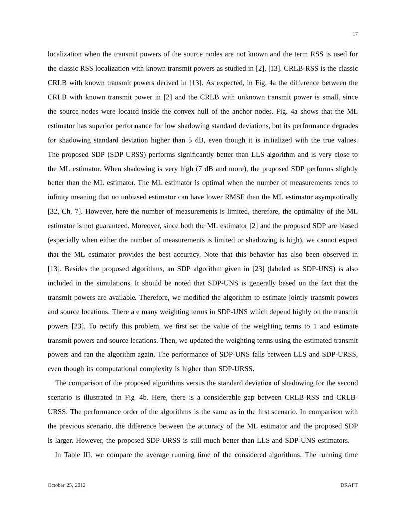
17
localization when the transmit powers of the source nodes are not known and the term RSS is used for
the classic RSS localization with known transmit powers as studied in [2], [13]. CRLB-RSS is the classic
CRLB with known transmit powers derived in [13]. As expected, in Fig. 4a the difference between the
CRLB with known transmit power in [2] and the CRLB with unknown transmit power is small, since
the source nodes were located inside the convex hull of the anchor nodes. Fig. 4a shows that the ML
estimator has superior performance for low shadowing standard deviations, but its performance degrades
for shadowing standard deviation higher than 5 dB, even though it is initialized with the true values.
The proposed SDP (SDP-URSS) performs significantly better than LLS algorithm and is very close to
the ML estimator. When shadowing is very high (7 dB and more),the proposed SDP performs slightly
better than the ML estimator. The ML estimator is optimal when the number of measurements tends to
infinity meaning that no unbiased estimator can have lower RMSE than the ML estimator asymptotically
[32, Ch. 7]. However, here the number of measurements is limited, therefore, the optimality of the ML
estimator is not guaranteed. Moreover, since both the ML estimator [2] and the proposed SDP are biased
(especially when either the number of measurements is limited or shadowing is high), we cannot expect
that the ML estimator provides the best accuracy. Note that this behavior has also been observed in
[13]. Besides the proposed algorithms, an SDP algorithm given in [23] (labeled as SDP-UNS) is also
included in the simulations. It should be noted that SDP-UNSis generally based on the fact that the
transmit powers are available. Therefore, we modified the algorithm to estimate jointly transmit powers
and source locations. There are many weighting terms in SDP-UNS which depend highly on the transmit
powers [23]. To rectify this problem, we first set the value ofthe weighting terms to 1 and estimate
transmit powers and source locations. Then, we updated the weighting terms using the estimated transmit
powers and ran the algorithm again. The performance of SDP-UNS falls between LLS and SDP-URSS,
even though its computational complexity is higher than SDP-URSS.
The comparison of the proposed algorithms versus the standard deviation of shadowing for the second
scenario is illustrated in Fig. 4b. Here, there is a considerable gap between CRLB-RSS and CRLB-
URSS. The performance order of the algorithms is the same as in the first scenario. In comparison with
the previous scenario, the difference between the accuracyof the ML estimator and the proposed SDP
is larger. However, the proposed SDP-URSS is still much better than LLS and SDP-UNS estimators.
In Table III, we compare the average running time of the considered algorithms. The running time
October 25, 2012 DRAFT

18
TABLE IIITHE AVERAGE RUNNING TIME OF THE CONSIDEREDALGORITHMS.
N = 10, |Aj | = 5, L = 95.CPU: INTEL CORE 2 DUO E7500 2.93 GHZ
Algorithm Iterations Time [ms]
ML 22 268.72SDP-URSS 19 218.34SDP-UNS 35 462.16LLS 1 11.81
is measured by averaging over 500 noise realizations when the first network with full connectivity is
considered and the standard deviation of the shadowing is set to 3 dB. LLS has the lowest complexity
and therefore the fastest running time. The required running time of the proposed SDP-URSS is about
20% lower than the ML estimator. From Table I, the complexity periteration for all algorithms is almost
identical for this network size (N = 10, |Aj | = 5). However, they require different numbers of iterations.
Moreover, we empirically computed the average number of iterations for the ML and SDP algorithms.
The average number of iterations for the ML and SDP-URSS were22 and 19, respectively. Consequently,
the running time of the ML and SDP-URSS is approximately 22 and 19 times higher than LLS (which
requires only one iteration). As mentioned in Section V, therunning time of the ML estimator depends
highly on the initialization. Here, the ML estimator has been initialized with the true values which cuts
down its running time and improves its performance. Later, we will discuss the effect of initialization
on the complexity and performance of the ML estimator. The computational of complexity of SDP-UNS
in [23] is almost the same as that of the proposed SDP-URSS. However, as mentioned above, SDP-
UNS should be run twice because of the estimation of the weighting terms. Therefore, the required
running time of SDP-UNS is nearly as twice as that of SDP-URSS. Thus, complexity and performance
are directly related for the considered algorithms, exceptfor SDP-UNS which was designed for known
transmit powers.
Fig. 5 illustrates the performance of the proposed SDP compared with the previously studied algorithm
in [13] (labeled as SDP-RSS) for the first scenario. Since SDP-RSS is based on the availability of source
transmit powers, the true values of the source nodes transmit powers were given to SDP-RSS in Fig. 5.
In SDP-RSS-WP, the same algorithm in [13] was used, however,the algorithm did not have the exact
value of the transmit powers and the value of -10 dBm was givento the algorithm as the reference power
October 25, 2012 DRAFT
19
1 2 3 4 5 6 7 80
0.5
1
1.5
2
2.5
3
3.5
4
Shadowing [dB]
RM
SE
[m]
SDP−URSSSDP−RSS−WPSDP−RSSSDP−RSS−S2SDP−RSS−S5CRLB−URSSCRLB−RSS
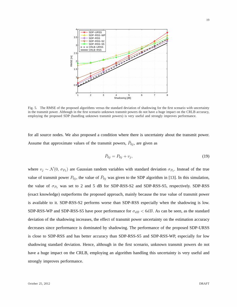
Fig. 5. The RMSE of the proposed algorithms versus the standard deviation of shadowing for the first scenario with uncertaintyin the transmit power. Although in the first scenario unknowntransmit powers do not have a huge impact on the CRLB accuracy,employing the proposed SDP (handling unknown transmit powers) is very useful and strongly improves performance.
for all source nodes. We also proposed a condition where there is uncertainty about the transmit power.
Assume that approximate values of the transmit powers,P0j , are given as
P0j = P0j + vj , (19)
wherevj ∼ N (0, σP0) are Gaussian random variables with standard deviationσP0
. Instead of the true
value of transmit powerP0j , the value ofP0j was given to the SDP algorithm in [13]. In this simulation,
the value ofσP0was set to 2 and 5 dB for SDP-RSS-S2 and SDP-RSS-S5, respectively. SDP-RSS
(exact knowledge) outperforms the proposed approach, mainly because the true value of transmit power
is available to it. SDP-RSS-S2 performs worse than SDP-RSS especially when the shadowing is low.
SDP-RSS-WP and SDP-RSS-S5 have poor performance forσdB < 6dB. As can be seen, as the standard
deviation of the shadowing increases, the effect of transmit power uncertainty on the estimation accuracy
decreases since performance is dominated by shadowing. Theperformance of the proposed SDP-URSS
is close to SDP-RSS and has better accuracy than SDP-RSS-S5 and SDP-RSS-WP, especially for low
shadowing standard deviation. Hence, although in the first scenario, unknown transmit powers do not
have a huge impact on the CRLB, employing an algorithm handling this uncertainty is very useful and
strongly improves performance.
October 25, 2012 DRAFT

20
1 2 3 4 5 6 7 80
1
2
3
4
5
6
7
8
9
Shadowing [dB]
RM
SE
[m]
SDP−URSSMLML−LLSML−RANDML−SDP−URSSCRLB−URSSCRLB−RSS
(a) The first scenario
1 2 3 4 5 6 7 80
1
2
3
4
5
6
7
8
9
Shadowing [dB]
RM
SE
[m]
SDP−URSSMLML−LLSML−RANDML−SDP−URSSCRLB−URSSCRLB−RSS
(b) The second scenario
Fig. 6. The RMSE of proposed algorithms versus the standard deviation of shadowing and different initializations for theML estimator. The initialization has a huge impact on the ML estimator performance. The proposed SDP algorithm providesasuitable initial point for the ML estimator if better accuracy is required.
C. Initialization
It is well-known that the performance of the ML estimator depends heavily on its initial solution, since
most implementations of the ML estimator are iterative. To further compare the proposed SDP and the ML
estimator, we initialized the solver of the ML estimator with different values. Fig. 6a and 6b illustrate the
RMSE of the proposed algorithms as a function of the standarddeviation of the shadowing with different
initial points for the solver of the ML estimator for the firstand second scenarios, respectively. The curve
labeled as ML stands for the ML estimator initialized with the true values, whereas ML-SDP, ML-LLS,
October 25, 2012 DRAFT

21
TABLE IVTHE AVERAGE RUNNING TIME OF THE ML ESTIMATOR WITH DIFFERENTINITIALIZATIONS .
Algorithm Iterations Time [ms]
ML 22 268.72ML-SDP 23 282.51ML-LLS 26 316.16ML-RAND 43 514.58
and ML-RAND stand for the ML estimator when its solver was initialized with the SDP solution, LLS
solution, and random values, respectively. Fig. 6 shows that in both scenarios, the ML estimator initialized
with the true values outperforms other algorithms as expected. However, the initial point can have a large
effect on ML accuracy. The proposed SDP algorithm offers better performance compared to ML-LLS
and ML-RAND, especially for large shadow fading standard deviation. It is interesting that when the ML
estimator is initialized with the solution of the proposed SDP (ML-SDP-URSS), we can achieve almost
the same accuracy as the ML algorithm initialized with the true solution. Therefore, although the proposed
SDP algorithm has excellent standalone performance, it canalso be used as an initial point for the ML
estimator when even better accuracy is required. Fig. 6 alsoshows that randomly initializing the ML
estimator yields extremely poor performance even at lowσdB values. Table IV shows the running time of
the ML estimator for different initializations. We can see that the initial point has a huge impact on not
only the performance of the ML estimator, but also the required number of iterations and the running time.
When the initial point is not sufficiently close to the globalminimum, the number of iterations increases
significantly. Moreover, there is no guarantee that the algorithm converges to the global minimum. This
is the major drawback of the ML estimator. In this case, an increase in running time (complexity) does
not result in performance improvement because of initialization; in fact the opposite is true.
D. Connectivity
In the previous simulations, we assumed that the network hasfull connectivity. However, this as-
sumption is not valid in all practical cases where the connections among sensors are limited. In this
section, we examine the first scenario but with limited connectivity. Fig. 7 shows the RMSE of the
proposed algorithms versus the number of connections when the shadowing standard deviation is 4 dB.
For instance, the value of 10 on the x-axis means that each source node is connected to the 10 closest
sensors, either anchor nodes or source nodes. The LLS estimator in (47) is no longer applicable here
October 25, 2012 DRAFT

22
6 7 8 9 10 11 12 13 141.5
2
2.5
3
3.5
4
4.5
Number of connections
RM
SE
[m]
SDP−URSSMLCRLB−URSSCRLB−RSS
Fig. 7. The RMSE of the proposed algorithms versus the numberof connections. The standard deviation of the shadowingis 4 dB. As the number of connections increases, the estimation accuracy improves. The proposed SDP algorithm has betterperformance than the ML estimator when the connectivity in the network is limited.
because in its formulation, each source node should be connected to at least four noncollinear anchor
nodes, but in low connectivity there is no guarantee that each source node can communicate with four
neighboring anchor nodes. Fig. 7 shows that by increasing the number of connections, the estimation
accuracy improves, as expected. Comparing the two CRLBs, weobserve that the unknown transmit
power has more effect on the CRLB accuracy when the network connectivity is limited. The proposed
SDP performs better than the ML estimator when the number of connections in the network is very low.
Potential reasons were previously mentioned in the description of Fig. 4. When the number of connections
is 6 or 7, the proposed SDP is slightly lower than CRLB. As mentioned previously in Section VI-B,
both SDP-URSS and ML estimators are biased (especially whenthe number of connections is limited)
and thus the CRLB cannot provide an absolute lower bound for them [2], [13], [41].
E. Path Loss Exponent (PLE)
In this section, we investigate the effect of imperfect PLE knowledge on the performance of the
proposed algorithms. The first scenario was considered for this simulation. However, we assume that the
estimators do not have the exact value of the PLE and instead they have an approximate value modeled
as
β = β +N (0, 1), (20)
October 25, 2012 DRAFT

23
1 2 3 4 5 6 7 80
1
2
3
4
5
6
7
Shadowing [dB]
RM
SE
[m]
LLSSDP−URSSMLCRLB−URSSCRLB−RSS
Fig. 8. The RMSE of the proposed algorithms versus the standard deviation of shadowing for the first scenario with uncertaintyin the PLE. Imperfect PLE decreases the performance of all algorithms, especially at lowσdB values. When the shadowing islarger than 6 dB, the proposed SDP is more robust against imperfect PLE than the ML estimator.
where β = 4 in our simulations. Fig. 8 shows the performance of the proposed algorithms in this
condition. The order of the algorithms remains unchanged compared to Fig. 4a. It is obvious that the
performance of all the algorithms degrades, especially at low values ofσdB . The proposed SDP-URSS
performs better than the ML estimator in the presence of PLE uncertainty when the shadowing standard
deviation is larger than 5 dB. Now, assume that we have an imperfect value of the PLE and the proposed
algorithms are computed based on the approach given in (18).Fig. 9 shows the estimate of the PLE
versus the number of iterations and different shadowing standard deviations for the proposed SDP in
(16). The true value of the PLE was set to 4 and we started the algorithm with the PLE of 3 and 5. It can
be seen from Fig. 8 that the RMSE performance of the proposed algorithms is poor at the low shadowing
standard deviations. However, as depicted in Fig. 9, by exploiting the iterative approach given in (18),
the imperfect PLE estimate converges to a value very close tothe true value for a small number of
iterations. It is worth mentioning that we have only plottedthe convergence of the PLE for the proposed
SDP in (16). However, the PLE convergence for the ML and LLS algorithms is more or less the same.
Our simulations show that once the PLE has converged, the RMSE of the proposed algorithms for the
source locations is almost identical to Fig. 4a.
October 25, 2012 DRAFT

24
1 2 3 4 5 6 7 8 9 10 113
3.2
3.4
3.6
3.8
4
4.2
4.4
4.6
4.8
5
Number of iterations
β
σdB = 0.1, β0 = 3
σdB = 0.1, β0 = 5
σdB = 3, β0 = 3
σdB = 3, β0 = 5
σdB = 6, β0 = 3
σdB = 6, β0 = 5
Fig. 9. The convergence rate of the PLE for the proposed SDP. The algorithm starts with the initial valueβ0. The true valueof β is 4. Once the PLE has converged, the proposed algorithms achieve performance nearly identical to what is achieved withperfect knowledge.
VII. C ONCLUSION
In this paper, cooperative RSS-based sensor localization with unknown and different transmit powers
was examined. The CRLB of the measurement model was derived and through computer simulations it
was shown that the effect of unknown transmit powers on the CRLB accuracy of the source locations
depends strongly on the network deployment geometry. A novel SDP technique was derived to estimate the
source transmit powers jointly with the source node locations. The complexity analyses of the considered
algorithms were presented. Simulation results demonstrated that the proposed SDP algorithm has excellent
performance, close to the original ML estimator in most conditions. Not only does the proposed SDP
exhibit good accuracy alone but also gives a good initial point for the ML estimator if further refinement
is required. We also introduced an approach for dealing withimperfect information about the path loss
exponent which can strongly impact the performance of RSS-based localization algorithms.
ACKNOWLEDGMENT
The authors would like to thank the associate editor, Prof. K. C. Ho, and the anonymous reviewers for
their valuable comments and suggestions which improved thequality of the paper.
October 25, 2012 DRAFT
25
APPENDIX A
CRAMER-RAO LOWER BOUND OF COOPERATIVE RSSLOCALIZATION
In this section, the CRLB of cooperative RSS localization with unknown transmit power is derived.
The CRLB defines a lower bound on the variance of any unbiased estimator and is employed as a
benchmark for evaluating the performance of estimators [32, Ch. 3], [1], [2], [13]. Since the transmit
power of the source nodes is not available to the estimator, it should also be taken into account as an
unknown parameter. Let us recall the vector of unknown parametersφ = [xT ,pT0 ]
T including the source
node locationsx = [xT1 ,x
T2 , . . . ,x
TN ]T and the source node transmit powersp0 = [P01, P02, . . . , P0N ]T .
From the measurement model in (11), the logarithm of the probability density function of the RSS
measurements is written as
ln p(p;φ) = k − σ−2dB(µ(φ)− p)T (µ(φ)− p), (21)
wherek is a constant which does not depend on the unknown parametersand p is the measurement
vector defined in (18).µ(φ) is the mean of the measurement vectorp defined as
µ(φ) =
µ1(φ)...
µN (φ)
, µj(φ) =
...
µij
...
i∈Aj∪Bj
(22)
where
µij = P0j − 10β log10 dij .
The CRLB of the unknown parameters are the diagonal elementsof the inverse of the Fisher information
matrix [32, Ch. 3]. The Fisher information matrix of the measurement model in (11) is obtained as [32,
Ch. 3]
J(φ) = σ−2dBF
TF, (23)
where
F =∂µ(φ)
∂φ=
F1
...
FN
, Fj =
...
fij...
i∈Aj∪Bj
October 25, 2012 DRAFT

26
and fij = [fyij, fpij],
fyij =
[
01×2(j−1),uTij ,01×2(N−j)
]
, i ∈ Aj
fyij =
[
01×2(j−1),uTij ,01×2(i−j−1),−uT
ij ,01×2(N−i)
]
, i ∈ Bj
fpij =
[
01×(j−1), 1,01×(N−j)
]
, i ∈ Aj ∪ Bj
uij =10β
ln 10
(yi − xj)
d2ij, i ∈ Aj
uij =10β
ln 10
(xi − xj)
d2ij, i ∈ Bj.
Therefore, the CRLB of the unknown parametersφ is computed as
CRLB([φ]r) =[
J−1(φ)]
r,r, r = 1, 2, . . . , 3N. (24)
APPENDIX B
L INEAR ESTIMATOR FORCOOPERATIVE RSS LOCALIZATION
In this work, we derived an SDP estimator to deal with the convergence problem of the ML estimator
and its complexity. Another solution for the ML convergenceproblem is to use a linear estimator which
has an analytical closed-form solution. To obtain a linear estimator, some approximations should be
applied to linearize the nonlinear measurement model of (1). Linear estimators for RSS localization have
been previously considered in the literature [4]. However,to the best of our knowledge, all of them
are based on availability of the transmitted power. Here, wederive a similar technique to the one used
in [4] with considering unknown transmit powers. Since linearizing the source-source measurements is
difficult, we propose a two-step algorithm. In the first step (called coarse estimation), we estimate the
location of each source node independently using only source-anchor measurements. Then, in the next
step (called fine estimation), we improve the accuracy of theestimated source locations by using source-
source measurements. The main drawback of this approach is that we require at least four source-anchor
measurements for each source node, otherwise we cannot find acoarse estimate for the source location
in the first step and therefore the second step will be not applicable. We now start by describing the first
step. Let us rewrite (7) for cooperative localization as (j ∈ S)
hijλij = αj + ǫij, i ∈ Aj, (25)
October 25, 2012 DRAFT

27
whereǫij = −nijαj(ln10)/5β is a zero-mean Gaussian random variable with variance(ln10)2α2jσ
2dB/25β
2.
Expanding the left-hand side (LHS) of (25) and rearranging gives
2λijyTi xj − λijx
Tj xj + αj = λijy
Ti yi + ǫij, i ∈ Aj . (26)
Let θ1,j = [xTj ,x
Tj xj , αj ]
T be the unknown vector to be estimated. Then (26) can be expressed in matrix
form as
G1,jθ1,j = h1,j + ǫ1,j, (27)
where
G1,j =
......
...
2λijyTi −λij 1
......
...
,
h1,j =
...
λijyTi yi
...
, ǫ1,j =
...
ǫij...
, i ∈ Aj ∪ Bj.
The LLS solution of (27) is [32, Ch. 4]
θ1,j = (GT1,jW1,jG1,j)
−1GT1,jW1,jh1,j , (28)
whereW1,j is the weighting matrix which is the inverse of the covariance matrix of the residual error
vectorǫ1,j
W1,j = E[ǫ1,jǫT1,j]
−1 = ((ln10)αjσdB/5β)−2
Im(j). (29)
wherem(j) = |Aj |. The covariance matrix of the estimated vectorθ1,j is [32, Ch. 4]
Cθ1,j= (GT
1,jW1,jG1,j)−1. (30)
The weighting matrixW1,j depends on the unknown parameterαj . Therefore, to compute the weighting
matrix, we can eliminate the value ofαj in (29) and determine the solution of (28). Sinceαj is a constant
factor inW1,j , its value does not change the solution ofθ1,j in (28). However, for further computations,
we can calculate the weighting matrixW1,j approximately byαj obtained from (28).
October 25, 2012 DRAFT

28
Since the elements of estimated parameters in (28) are dependent, one method to improve the estimation
accuracy, called correction technique [5], [17], [42], is to take this relation between elements ofθ1,j into
account. Here we extend the correction technique to our problem. The unknown vectorθ1,j can be
expressed as
θ1,j = θ1,j +∆θ1,j, (31)
where∆θ1,j is the estimation error. Squaring the first two elements of (31) (element-wise) yields
[θ1,j]21 = [θ1,j ]
21 + 2[θ1,j ]1[∆θ1,j ]1 + [∆θ1,j ]
21
≃ [θ1,j ]21 + 2[θ1,j ]1[∆θ1,j ]1,
[θ1,j]22 = [θ1,j ]
22 + 2[θ1,j ]2[∆θ1,j ]2 + [∆θ1,j ]
22
≃ [θ1,j ]22 + 2[θ1,j ]2[∆θ1,j ]2, (32)
where we assume that the estimation error∆θ1,j is sufficiently small. Now, consider the following
expressions [17]
G2θ2,j = h2,j + ǫ2,j, (33)
whereθ2,j = [a2j , b2j , αj ]
T and
G2 =
1 0 0
0 1 0
1 1 0
0 0 1
, h2,j =
[θ1,j ]21
[θ1,j ]22
[θ1,j ]3
[θ1,j ]4
, ǫ2,j = −Bj∆θ1,j,
andBj = diag{2[θ1,j]1, 2[θ1,j ]2, 1, 1}. The LLS solution of (33) is [32, Ch. 4]
θ2,j = (GTW2,jG)−1GTW2,jh2,j , (34)
whereW2,j is the weighting matrix equal to the inverse of the covariance matrix of the residual error
vectorǫ2,j
W2,j = E[ǫ2,jǫT2,j]
−1 =(
BTj Cθ1,j
Bj
)−1, (35)
whereCθ1,jis computed in (30). It should be noted that the weighting matrix W2,j depends on the
October 25, 2012 DRAFT

29
unknown parametersθ1. Therefore, the weighting matrix is approximately calculated by availableθ1
rather thanθ1. Our simulations show that the accuracy degradation due to the approximation is not
significant. The covariance matrix of the estimated vectorθ2,j is [32, Ch. 4]
Cθ2,j= (GT
2 W2,jG2)−1. (36)
Finally, the estimation of the source locationxj = [aj , bj ]T is [17], [18], [43]
aj = sgn([θ1,j]1)
√
|[θ2,j ]1|
bj = sgn(|[θ1,j ]2|)√
|[θ2,j]2|, (37)
wheresgn(z) = z/|z| is the sign function. The covariance matrix of the estimatedsource locationxj is
computed as [18], [43]
Cxj= DT
j [Cθ2,j]1:2,1:2Dj, (38)
whereDj =12diag{|aj |−1, |bj |−1} and [A]1:n,1:m denotes the upper-leftn×m part of matrixA.
Now we continue describing the second step using both source-source and source-anchor measurements.
The relationships between the estimated and the true value of the source location and the transmit power
of the source node are
xj = xj −∆xj ,
P0j = P0j −∆P0j , (39)
whereP0j = 5β log10(αj) (αj = [θ2,j]3 is computed for each source node from (34)),∆xj and∆P0j are
the estimation error of the source location and the source transmit power, respectively. Equation (11) is
a function of the unknown parametersxj andP0j . We substitute (39) forxj andP0j in (11). Therefore,
∆P0j and∆xj are the new unknown parameters to be estimated in (11).
Pij = (P0j − P0j) (40)
− 10β log10 ‖yi − (xj −∆xj)‖+ nij, i ∈ Aj,
Pij = (P0j −∆P0j)
− 10β log10 ‖(xi −∆xi)− (xj −∆xj)‖+ nij, i ∈ Bj.
October 25, 2012 DRAFT

30
Taking the power of 10 on both sides of (40) and rearranging yields
ξij∆αj10nij/10β = ‖yi − (xj −∆xj)‖, i ∈ Aj, (41)
ξij∆αj10nij/10β = ‖(xi −∆xi)− (xj −∆xj)‖, i ∈ Bj,
whereξij , 10(P0j−Pij)/10β and∆αj , 10−∆P0j/10β . By using the first-order Taylor series approximation
for the third element of the LHS and the element of the RHS, (41) turns into
ξij∆αj(1 +ln 10
10βnij) = dij − uT
ij∆xj, i ∈ Aj, (42)
ξij∆αj(1 +ln 10
10βnij) = dij − uT
ij∆xj + uTij∆xi, i ∈ Bj,
where
uij =(xj − yi)
dij, dij = ‖yi − xj‖, i ∈ Aj,
uij =(xj − xi)
dij, dij = ‖xi − xj‖, i ∈ Bj.
Rearranging (42) gives
uTij∆xj + ξij∆αj = dij + ǫij, i ∈ Aj,
−uTij∆xi + uT
ij∆xj + ξij∆αj = dij + ǫij, i ∈ Bj, (43)
whereǫij , (ln10) ξij∆αjnij/10β. Let ∆θ3 = [∆xT1 , . . . ,∆xT
N ,∆α1, . . . ,∆αN ]T be unknown param-
eters to be estimated. We can write (43) in matrix form as
G3∆θ3 = h3 + ǫ3, (44)
where
G3 =
G3,1
...
G3,N
, h3 =
h3,1
...
h3,N
, ǫ3 =
ǫ3,1...
ǫ3,N
,
October 25, 2012 DRAFT

31
G3,j =
...
gij...
, h3,j =
...
dij...
, ǫ3,j =
...
ǫij...
i∈Aj∪Bj
andgij = [gyij , g
pij ],
gyij =
[
01×2(j−1), uTij ,01×2(N−j)
]
, i ∈ Aj
gyij =
[
01×2(j−1), uTij ,01×2(i−j−1),−uT
ij,01×2(N−i)
]
, i ∈ Bj
gpij =
[
01×(j−1), ξij,01×(N−j)
]
, i ∈ Aj ∪ Bj
Since as prior knowledge, we know that the unknown vector∆θ3 is not too large, (44) can be solved
by the Tikhonov-regularized LS formulation in which the cost function includes the weighted squared
norm of∆θ3 to keep it as small as possible. The Tikhonov-regularized LSsolution of (44) is obtained
as [44], [26, Ch. 6]
∆θ3 = argmin∆θ3∈R3N
‖G3∆θ3 − h3‖2 + δ‖∆θ3‖2, (45)
whereδ is a regularization parameter controlling the trade-off between‖G3∆θ3 − h3‖2 and ‖∆θ3‖2.
The closed-form solution of (45) is given by [26, Ch. 6]
∆θ3 =(
GT3 G3 + δIL
)−1GT
3 h3. (46)
Finally, the location of each source node is determined as
xj = xj −∆xj, j ∈ S. (47)
APPENDIX C
COMPLEXITY ANALYSIS OF THE ALGORITHMS
The computational complexity of the considered algorithmsbased on the required number of flops is
derived in this section. We assume that an addition, subtraction, multiplication, division, or square root
operation in the real domain can be computed by one flop [45], [46]. For simplicity, we keep only the
leading terms of the complexity expressions. We derive the complexity of cooperative approaches which
includes non-cooperative case as a special case (N = 1). Note that the worst-case complexity is derived
October 25, 2012 DRAFT

32
without any attempt to optimize computations to take advantage of, e.g., the structure of matrices. The
complexity of the considered algorithms is computed as a function of N , the number of source nodes,
M , the number of anchor nodes, andL =∑
j∈S |Aj |+ |Bj|, the total number of connections. Note that
for a network with full connectivity, we haveL = N(M + (N − 1)/2).
A. Maximum Likelihood
As previously mentioned, the ML estimator is nonlinear and nonconvex. Therefore, ML complexity
highly depends on the solution method. In addition, the complexity of every method also depends on
many parameters, e.g., the number of iterations, the initial point, or the solution accuracy. Gauss-Newton
(GN) is the one of the most popular methods used in solving nonlinear optimization problems [32, Ch.
8]. GN is an iterative technique and requires initialization. Assuming a nonlinear problem with a set of
m equations andn unknown variables, the asymptotic computational complexity (m ≫ n) of the GN
method in each iteration isO(m3) [47]. The number of iterations depends highly on the initialpoint
and required accuracy. AssumingO(k) iterations on average is required to solve a specific problem, the
total complexity of the GN method isO(km3). For the proposed ML, we havem = L, andn = 3N .
Consequently, the asymptotic complexity of the ML estimator in (12) is
ML Complexity ≃ O(kL3). (48)
B. Semidefinite Programming
Consider the general form of a semidefinite programming problem [25]
minimizex
cTx
subject to F(x) � 0,(49)
wherex ∈ Rm and
F(x) = F0 +
m∑
i=1
xiFi.
The available data includes the vectorc ∈ Rm andm+ 1 symmetric matricesF0, . . . ,Fm ∈ R
n×n. An
SDP problem can be solved by iterative optimization techniques, e.g., interior-point methods [25], [26].
The worst-case computational complexity of solving SDP in each iteration isO(m2n2) [25]. The number
of iterations is also bounded byO(√n log(1/ǫ)), whereǫ is the accuracy of SDP solution [25], [34]. For
October 25, 2012 DRAFT

33
the proposed SDP, we havem ≃ L+ 3N andn ≃ N . Therefore, the complexity of the SDP in (16) is
SDP Complexity≃ O(√N(L+ 3N)2N2 log(1/ǫ)). (50)
C. Linear estimator
Consider a weighted linear least squares problem with a set of m equations andn unknown variables
defined as [32, Ch. 5]
θ = (GTWG)−1GTWh, (51)
whereθ ∈ Rn, G ∈ R
m×n, W ∈ Rm×m, andh ∈ R
m. Computingθ includes five matrix multiplications
and one matrix inversion. Therefore, the computational complexity of (51) isO(2m2n+mn2+mn+n3+
n2) [45], [48]. Assumingm ≫ 2n, the complexity of (51) is upper bounded byO(m3). The complexity
of the proposed LLS algorithms can be simply expressed as follows,
TABLE VCOMPLEXITY OF LLS ALGORITHMS.
Algorithm m n Complexity
LLS in (28) |Aj | 4 O(8|Aj |2 + 20|Aj |+ 80)LLS in (34) 4 3 O(180)
LLS in (46) L 3N O(6L2N + 9LN2)PLE in (18) L N + 1 O(2L2(N + 1) + L(N + 1)2)
The cooperative LLS algorithm includes (28), (34) which arecalculated forN source nodes and (46).
Therefore, from Table V, the total computational complexity of the cooperative LLS approach is
LLS Complexity ≃ O(6L2N + 9LN2 +∑
j∈S
8|Aj |2). (52)
REFERENCES
[1] N. Patwari, J. N. Ash, S. Kyperountas, A. O. Hero III, R. L.Moses, and N. S. Correal, “Locating the nodes: Cooperative
localization in wireless sensor networks,”IEEE Signal Process. Mag., vol. 22, no. 4, pp. 54–69, July 2005.
[2] N. Patwari, A. O. Hero III, M. Perkins, N. S. Correal, and R. J. O’Dea, “Relative location estimation in wireless sensor
networks,” IEEE Trans. Signal Process., vol. 51, no. 8, pp. 2137–2148, August 2003.
[3] X. Li, “Collaborative localization with received-signal strength in wireless sensor networks,”IEEE Trans. Veh. Technol.,
vol. 56, no. 6, pp. 3807–3817, November 2007.
[4] H. C. So and L. Lin, “Linear least squares approach for accurate received signal strength based source localization,” IEEE
Trans. Signal Process., vol. 59, no. 8, pp. 4035–4040, August 2011.
October 25, 2012 DRAFT

34
[5] I. Guvenc and C.-C. Chong, “A survey on TOA based wirelesslocalization and NLOS mitigation techniques,”IEEE
Commun. Surveys Tuts., vol. 11, no. 3, pp. 107–124, 2009.
[6] S. Venkatesh and R. M. Buehrer, “NLOS mitigation using linear programming in ultrawideband location-aware networks,”
IEEE Trans. Veh. Technol., vol. 56, no. 5, pp. 3182–3198, September 2007.
[7] A. Catovic and Z. Sahinoglu, “The Cramer-Rao bounds of hybrid TOA/RSS and TDOA/RSS location estimation schemes,”
IEEE Commun. Lett., vol. 8, no. 10, pp. 626–628, October 2004.
[8] L. Yang and K. C. Ho, “An approximately efficient TDOA localization algorithm in closed-form for locating multiple
disjoint sources with erroneous sensor positions,”IEEE Trans. Signal Process., vol. 57, no. 12, pp. 4598–4615, December
2009.
[9] M. Sun and K. C. Ho, “An asymptotically efficient estimator for TDOA and FDOA positioning of multiple disjoint sources
in the presence of sensor location uncertainties,”IEEE Trans. Signal Process., vol. 59, no. 7, pp. 3434–3440, July 2011.
[10] R. M. Vaghefi, M. R. Gholami, and E. G. Strom, “Bearing-only target localization with uncertainties in observer position,”
in Proc. IEEE PIMRC, September 2010, pp. 238–242.
[11] L. Cong and W. Zhuang, “Hybrid TDOA/AOA mobile user location for wideband CDMA cellular systems,”IEEE Trans.
Wireless Commun., vol. 1, no. 3, pp. 439–447, July 2002.
[12] K. W. Cheung, H. C. So, W.-K. Ma, and Y. T. Chan, “A constrained least squares approach to mobile positioning: Algorithms
and optimality,”EURASIP J. Appl. Signal Process., pp. 1–23, 2006.
[13] R. W. Ouyang, A. K.-S. Wong, and C.-T. Lea, “Received signal strength-based wireless localization via semidefinite
programming: Noncooperative and cooperative schemes,”IEEE Trans. Veh. Technol., vol. 59, no. 3, pp. 1307–1318, March
2010.
[14] Y.-T. Chan, H. Y. C. Hang, and P. chung Ching, “Exact and approximate maximum likelihood localization algorithms,”
IEEE Trans. Veh. Technol., vol. 55, no. 1, pp. 10–16, Januray 2006.
[15] X. Sheng and Y.-H. Hu, “Maximum likelihood multiple-source localization using acoustic energy measurements with
wireless sensor networks,”IEEE Trans. Signal Process., vol. 53, no. 1, pp. 44–53, Januray 2005.
[16] C. Meng, Z. Ding, and S. Dasgupta, “A semidefinite programming approach to source localization in wireless sensor
networks,” IEEE Signal Process. Lett., vol. 15, pp. 253–256, 2008.
[17] C. Meesookho, U. Mitra, and S. Narayanan, “On energy-based acoustic source localization for sensor networks,”IEEE
Trans. Signal Process., vol. 56, no. 1, pp. 365–377, January 2008.
[18] M. Sun and K. C. Ho, “Successive and asymptotically efficient localization of sensor nodes in closed-form,”IEEE Trans.
Signal Process., vol. 57, no. 11, pp. 4522–4537, November 2009.
[19] R. M. Vaghefi, M. R. Gholami, and E. G. Strom, “RSS-basedsensor localization with unknown transmit power,” inProc.
IEEE ICASSP, May 2011, pp. 2480–2483.
[20] P. Biswas, T.-C. Liang, K.-C. Toh, Y. Ye, and T.-C. Wang,“Semidefinite programming approaches for sensor network
localization with noisy distance measurements,”IEEE Trans. Autom. Sci. Eng., vol. 3, no. 4, pp. 360–371, October 2006.
[21] A. M.-C. So and Y. Ye, “Theory of semidefinite programming for sensor network localization,”Math. Program., Series B,
vol. 109, no. 2–3, pp. 367–384, October 2007.
October 25, 2012 DRAFT

35
[22] R. M. Vaghefi and R. M. Buehrer, “Cooperative sensor localization with NLOS mitigation using semidefinite programming,”
in Proc. 9th Workshop on Positioning, Navigation and Communication (WPNC), March 2012.
[23] G. Wang and K. Yang, “A new approach to sensor node localization using RSS measurements in wireless sensor networks,”
IEEE Trans. Wireless Commun., vol. 10, no. 5, pp. 1389–1395, May 2011.
[24] E. Xu, Z. Ding, and S. Dasgupta, “Reduced complexity semidefinite relaxation algorithms for source localization based
on time difference of arrival,”IEEE Trans. Mob. Comput., vol. 10, no. 9, pp. 1276–1282, September 2011.
[25] L. A. Vandenberghe and S. B. Boyd, “Semidefinite programming,” SIAM Rev., vol. 38, no. 1, pp. 49–95, March 1996.
[26] S. Boyd and L. Vandenberghe,Convex Optimization. Cambridge, UK: Cambridge University Press, 2004.
[27] S. Kim, H. Jeon, and J. Ma, “Robust localization with unknown transmission power for cognitive radio,” inProc. IEEE
MILCOM, October 2007, pp. 1–6.
[28] J. H. Lee and R. M. Buehrer, “Location estimation using differential RSS with spatially correlated shadowing,” inProc.
IEEE GLOBECOM, December 2009, pp. 1–6.
[29] G. Wang and K. Yang, “Efficient semidefinite relaxation for energy-based source localization in sensor networks,” in Proc.
IEEE ICASSP, 2009, pp. 2257–2260.
[30] M. R. Gholami, M. Rydstrom, and E. G. Strom, “Positioning of node using plane projection onto convex sets,” inProc.
IEEE WCNC, April 2010, pp. 1–5.
[31] C. Liu, K. Wu, and T. He, “Sensor localization with ring overlapping based on comparison of received signal strength
indicator,” in Proc. IEEE MASS, October 2004, pp. 516–518.
[32] S. M. Kay, Fundamentals of Statistical Signal Processing: Estimation Theory. Upper Saddle River, NJ: Prentice-Hall,
1993.
[33] W. H. Foy, “Position-location solution by Taylor-series estimation,”IEEE Trans. Aerosp. Electron. Syst., vol. 12, no. 3,
pp. 187–194, March 1976.
[34] J. F. Sturm, “Using SeDuMi 1.02, a MATLAB toolbox for optimization over symmetric cones,” 1998.
[35] R. H. Tutuncu, K. C. Toh, and M. J. Todd, “Solving semidefinite-quadratic-linear programs using SDPT3,”Math. Program.,
vol. 95, no. 2, pp. 189–217, February 2003.
[36] J. Kivinen, X. Zhao, and P. Vainikainen, “Empirical characterization of wideband indoor radio channel at 5.3 GHz,”IEEE
Trans. Antennas Propag., vol. 49, no. 8, pp. 1192–1203, August 2001.
[37] X. Li, “RSS-based location estimation with unknown pathloss model,”IEEE Trans. Wireless Commun., vol. 5, no. 12, pp.
3626–3633, December 2006.
[38] P. Biswas, T.-C. Lian, T.-C. Wang, and Y. Ye, “Semidefinite programming based algorithms for sensor network localization,”
ACM Trans. Sen. Netw., vol. 2, no. 2, pp. 188–220, May 2006.
[39] M. Grant and S. Boyd, “CVX: Matlab software for disciplined convex programming, version 1.21,” http://cvxr.com/cvx,
May 2010.
[40] D. Torrieri, “Statistical theory of passive location systems,”IEEE Trans. Aerosp. Electron. Syst., vol. 20, no. 2, pp. 183–198,
July 1984.
[41] T. Jia and R. M. Buehrer, “On the optimal performance of collaborative position location,”IEEE Trans. Wireless Commun.,
vol. 9, no. 1, pp. 374–383, January 2010.
October 25, 2012 DRAFT

36
[42] Y. T. Chan and K. C. Ho, “A simple and efficient estimator for hyperbolic location,”IEEE Trans. Signal Process., vol. 42,
no. 8, pp. 1905–1915, August 1994.
[43] M. R. Gholami, S. Gezici, E. G. Strom, and M. Rydstrom,“Positioning algorithms for cooperative networks in the presence
of an unknown turn-around time,” inProc. IEEE SPAWC, June 2011, pp. 166–170.
[44] ——, “Hybrid TW-TOA/TDOA positioning algorithms for cooperative wireless networks,” inProc. IEEE ICC, June 2011,
pp. 1–5.
[45] G. Golub and C. F. V. Loan,Matrix computations, 3rd ed. Johns Hopkins University Press, 1996.
[46] M. R. Gholami, S. Gezici, and E. G. Strom, “Improved position estimation using hybrid TW-TOA and TDOA in cooperative
networks,” IEEE Trans. Signal Process., vol. 60, no. 7, pp. 3770–3785, July 2012.
[47] C. A. Floudas and P. M. Pardalos,Encyclopedia of Optimization, 2nd ed. New York, NY: Springer-Verlag, 2009.
[48] S. Arora and B. Barak,Computational Complexity: A Modern Approach. Cambridge University Press, 2009.
October 25, 2012 DRAFT