Embed Size (px)
Citation preview

Challenges for Worst-case Execution Time Analysis of Multi-core Architectures Jan Reineke @
Intel, Braunschweig April 29, 2013
computer science
saarlanduniversity

Jan Reineke, Saarland 2
The Context: Hard Real-Time Systems
Safety-critical applications: ¢ Avionics, automotive, train industries, manufacturing
¢ Embedded controllers must finish their tasks within given time bounds.
¢ Developers would like to know the Worst-Case Execution Time (WCET) to give a guarantee.
computer science
saarlanduniversityHard Real-Time Systems
Safety-critical applications:Avionics, automotive, train industries, manufacturing control
Side airbag in car Crankshaft-synchronous tasksReaction in < 10 msec Reaction in < 45 µsec
Embedded controllers must finish their tasks within given time
bounds.Developers would like to know the Worst-Case Execution Time
(WCET) to give a guarantee.
Jan Reineke Timing Analysis and Timing Predictability 11. Februar 2013 4 / 38
Side airbag in car Reaction in < 10 msec
Crankshaft-synchronous tasks Reaction in < 45 microsec

Jan Reineke, Saarland 3
The Timing Analysis Problem
Embedded Software
Timing Requirements ?
Our Vision: PRET Machines
PREcision-Timed processors: Performance & Predicability
+ = PRET
(Image: John Harrison’s H4, first clock to solve longitude problem)
Precision-Timed (PRET) Machines – p. 11/19
Microarchitecture
+

Jan Reineke, Saarland 4
computer science
saarlanduniversityWhat does the execution time depend on?
1 The input, determining which path is taken through the program.2 The state of the hardware platform:
I Due to caches, pipelines, speculation, etc.3 Interferences from the environment:
I External interferences as seen from the analyzed task on sharedbusses, caches, memory.
Simple CPU
Memory
Jan Reineke Timing Analysis and Timing Predictability 11. Februar 2013 6 / 38
What does the execution time depend on?
¢ The input, determining which path is taken through the program.
¢ The state of the hardware platform: l Due to caches, pipelining, speculation, etc.
¢ Interference from the environment: l External interference as seen from the analyzed
task on shared busses, caches, memory.

Jan Reineke, Saarland 5
computer science
saarlanduniversityWhat does the execution time depend on?
1 The input, determining which path is taken through the program.2 The state of the hardware platform:
I Due to caches, pipelines, speculation, etc.3 Interferences from the environment:
I External interferences as seen from the analyzed task on sharedbusses, caches, memory.
Simple CPU
Memory
Jan Reineke Timing Analysis and Timing Predictability 11. Februar 2013 6 / 38
computer science
saarlanduniversityWhat does the execution time depend on?
1 The input, determining which path is taken through the program.2 The state of the hardware platform:
I Due to caches, pipelines, speculation, etc.3 Interferences from the environment:
I External interferences as seen from the analyzed task on sharedbusses, caches, memory.
Complex CPU(out-of-order execution,
branch prediction, etc.)
MainMemory
L1 Cache
Jan Reineke Timing Analysis and Timing Predictability 11. Februar 2013 6 / 38
What does the execution time depend on?
¢ The input, determining which path is taken through the program.
¢ The state of the hardware platform: l Due to caches, pipelining, speculation, etc.
¢ Interference from the environment: l External interference as seen from the analyzed
task on shared busses, caches, memory.

Jan Reineke, Saarland 6
computer science
saarlanduniversityWhat does the execution time depend on?
1 The input, determining which path is taken through the program.2 The state of the hardware platform:
I Due to caches, pipelines, speculation, etc.3 Interferences from the environment:
I External interferences as seen from the analyzed task on sharedbusses, caches, memory.
Simple CPU
Memory
Jan Reineke Timing Analysis and Timing Predictability 11. Februar 2013 6 / 38
computer science
saarlanduniversityWhat does the execution time depend on?
1 The input, determining which path is taken through the program.2 The state of the hardware platform:
I Due to caches, pipelines, speculation, etc.3 Interferences from the environment:
I External interferences as seen from the analyzed task on sharedbusses, caches, memory.
Complex CPU(out-of-order execution,
branch prediction, etc.)
MainMemory
L1 Cache
Jan Reineke Timing Analysis and Timing Predictability 11. Februar 2013 6 / 38
computer science
saarlanduniversityWhat does the execution time depend on?
1 The input, determining which path is taken through the program.2 The state of the hardware platform:
I Due to caches, pipelines, speculation, etc.3 Interferences from the environment:
I External interferences as seen from the analyzed task on sharedbusses, caches, memory.
Complex CPU
L1 Cache
Complex CPU
L1 Cache
...L2
CacheMain
Memory
Jan Reineke Timing Analysis and Timing Predictability 11. Februar 2013 6 / 38
What does the execution time depend on?
¢ The input, determining which path is taken through the program.
¢ The state of the hardware platform: l Due to caches, pipelining, speculation, etc.
¢ Interference from the environment: l External interference as seen from the analyzed
task on shared busses, caches, memory.
Jan Reineke, Saarland 7
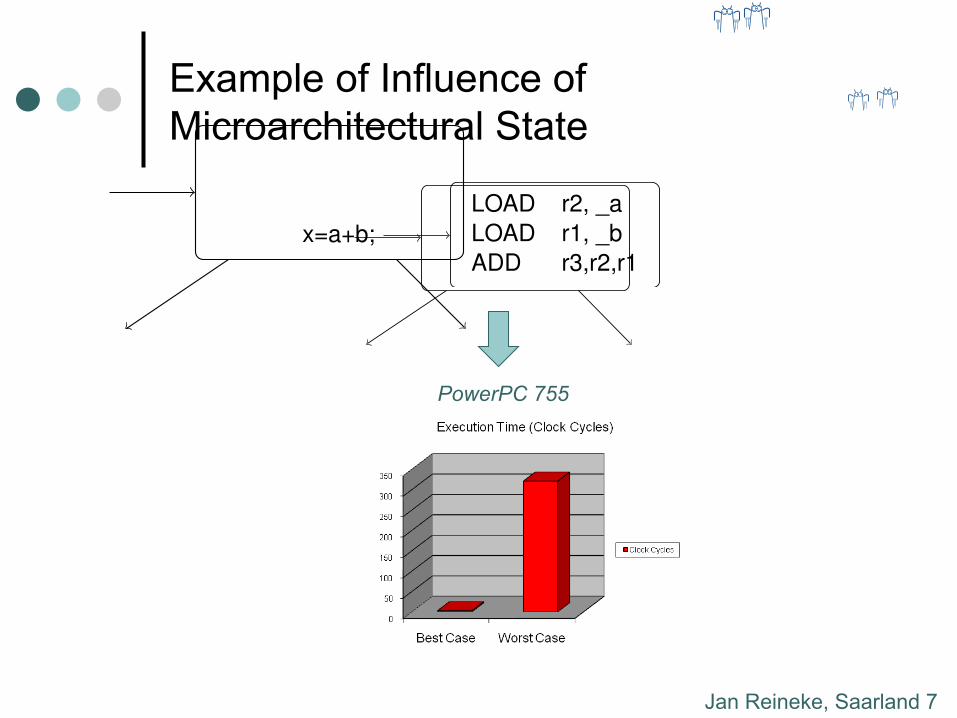
Example of Influence of Microarchitectural State
PowerPC 755
Reineke et al., Berkeley 5
Example of Influence of
Microarchitectural State computer science
saarlanduniversityAccess Time
x=a+b;LOAD r2, _aLOAD r1, _bADD r3,r2,r1
MPC5xx PPC755
Reinhard Wilhelm Timing Analysis and Timing Predictability Tutorial ISCA 2010 5 / 63
computer science
saarlanduniversityAccess Time
x=a+b;LOAD r2, _aLOAD r1, _bADD r3,r2,r1
MPC5xx PPC755
Reinhard Wilhelm Timing Analysis and Timing Predictability Tutorial ISCA 2010 5 / 63
Motorola PowerPC 755
Courtesy of Reinhard Wilhelm.

Jan Reineke, Saarland 8
Example of Influence of Corunning Tasks in Multicores
Radojkovic et al. (ACM TACO, 2012) on Intel Atom and Intel Core 2 Quad:
up to 14x slow-down due to interference on shared L2 cache and memory controller

Jan Reineke, Saarland 9
Challenges
1. Modeling How to construct sound timing models?
2. Analysis How to precisely & efficiently bound the WCET?
3. Design How to design microarchitectures that enable precise & efficient WCET analysis?

Jan Reineke, Saarland 10
The Modeling Challenge
Timing model = Formal specification of microarchitecture’s timing
Incorrect timing model
à possibly incorrect WCET bound.
Our Vision: PRET Machines
PREcision-Timed processors: Performance & Predicability
+ = PRET
(Image: John Harrison’s H4, first clock to solve longitude problem)
Precision-Timed (PRET) Machines – p. 11/19
Timing Model
Micro-architecture
?

Jan Reineke, Saarland 11
Current Process of Deriving Timing Model Our Vision: PRET Machines
PREcision-Timed processors: Performance & Predicability
+ = PRET
(Image: John Harrison’s H4, first clock to solve longitude problem)
Precision-Timed (PRET) Machines – p. 11/19
Micro-architecture
Timing Model
?

Jan Reineke, Saarland 12
Current Process of Deriving Timing Model Our Vision: PRET Machines
PREcision-Timed processors: Performance & Predicability
+ = PRET
(Image: John Harrison’s H4, first clock to solve longitude problem)
Precision-Timed (PRET) Machines – p. 11/19
Micro-architecture
Timing Model
?

Jan Reineke, Saarland 13
Current Process of Deriving Timing Model Our Vision: PRET Machines
PREcision-Timed processors: Performance & Predicability
+ = PRET
(Image: John Harrison’s H4, first clock to solve longitude problem)
Precision-Timed (PRET) Machines – p. 11/19
Micro-architecture
Timing Model
?

Jan Reineke, Saarland 14
Current Process of Deriving Timing Model Our Vision: PRET Machines
PREcision-Timed processors: Performance & Predicability
+ = PRET
(Image: John Harrison’s H4, first clock to solve longitude problem)
Precision-Timed (PRET) Machines – p. 11/19
Micro-architecture
Timing Model
?

Jan Reineke, Saarland 15
Current Process of Deriving Timing Model
à Time-consuming, and à error-prone.
Our Vision: PRET Machines
PREcision-Timed processors: Performance & Predicability
+ = PRET
(Image: John Harrison’s H4, first clock to solve longitude problem)
Precision-Timed (PRET) Machines – p. 11/19
Micro-architecture
Timing Model
?

Jan Reineke, Saarland 16
Current Process of Deriving Timing Model
à Time-consuming, and à error-prone.
Our Vision: PRET Machines
PREcision-Timed processors: Performance & Predicability
+ = PRET
(Image: John Harrison’s H4, first clock to solve longitude problem)
Precision-Timed (PRET) Machines – p. 11/19
Micro-architecture
Timing Model
?

Jan Reineke, Saarland 17
1. Future Process of Deriving Timing Model Our Vision: PRET Machines
PREcision-Timed processors: Performance & Predicability
+ = PRET
(Image: John Harrison’s H4, first clock to solve longitude problem)
Precision-Timed (PRET) Machines – p. 11/19
Micro-architecture
Timing Model
VHDL Model

Jan Reineke, Saarland 18
1. Future Process of Deriving Timing Model Our Vision: PRET Machines
PREcision-Timed processors: Performance & Predicability
+ = PRET
(Image: John Harrison’s H4, first clock to solve longitude problem)
Precision-Timed (PRET) Machines – p. 11/19
Micro-architecture
Timing Model
VHDL Model
Derive timing model automatically from formal specification of microarchitecture.
à Less manual effort, thus less time-consuming, and à provably correct.

Jan Reineke, Saarland 19
1. Future Process of Deriving Timing Model Our Vision: PRET Machines
PREcision-Timed processors: Performance & Predicability
+ = PRET
(Image: John Harrison’s H4, first clock to solve longitude problem)
Precision-Timed (PRET) Machines – p. 11/19
Micro-architecture
Timing Model
VHDL Model
Derive timing model automatically from formal specification of microarchitecture.
à Less manual effort, thus less time-consuming, and à provably correct.

Jan Reineke, Saarland 20
1. Future Process of Deriving Timing Model Our Vision: PRET Machines
PREcision-Timed processors: Performance & Predicability
+ = PRET
(Image: John Harrison’s H4, first clock to solve longitude problem)
Precision-Timed (PRET) Machines – p. 11/19
Micro-architecture
Timing Model
VHDL Model
Derive timing model automatically from formal specification of microarchitecture.
à Less manual effort, thus less time-consuming, and à provably correct.
Jan Reineke, Saarland 21
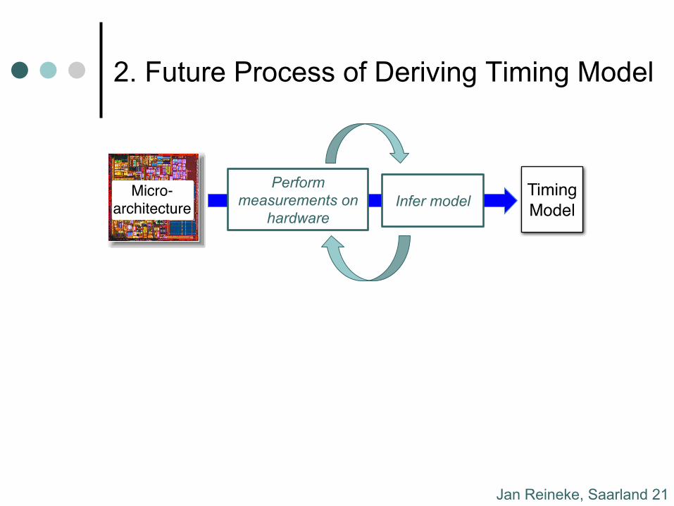
2. Future Process of Deriving Timing Model Our Vision: PRET Machines
PREcision-Timed processors: Performance & Predicability
+ = PRET
(Image: John Harrison’s H4, first clock to solve longitude problem)
Precision-Timed (PRET) Machines – p. 11/19
Micro-architecture
Timing Model
Perform measurements on
hardware
Infer model

Jan Reineke, Saarland 22
2. Future Process of Deriving Timing Model Our Vision: PRET Machines
PREcision-Timed processors: Performance & Predicability
+ = PRET
(Image: John Harrison’s H4, first clock to solve longitude problem)
Precision-Timed (PRET) Machines – p. 11/19
Micro-architecture
Timing Model
Perform measurements on
hardware
Derive timing model automatically from measurements on the hardware using ideas from automata learning.
à No manual effort, and à (under certain assumptions) provably correct. à Also useful to validate assumptions about microarch.
Infer model

Jan Reineke, Saarland 23
2. Future Process of Deriving Timing Model Our Vision: PRET Machines
PREcision-Timed processors: Performance & Predicability
+ = PRET
(Image: John Harrison’s H4, first clock to solve longitude problem)
Precision-Timed (PRET) Machines – p. 11/19
Micro-architecture
Timing Model
Perform measurements on
hardware
Derive timing model automatically from measurements on the hardware using ideas from automata learning.
à No manual effort, and à (under certain assumptions) provably correct. à Also useful to validate assumptions about microarch.
Infer model

Jan Reineke, Saarland 24
2. Future Process of Deriving Timing Model Our Vision: PRET Machines
PREcision-Timed processors: Performance & Predicability
+ = PRET
(Image: John Harrison’s H4, first clock to solve longitude problem)
Precision-Timed (PRET) Machines – p. 11/19
Micro-architecture
Timing Model
Perform measurements on
hardware
Derive timing model automatically from measurements on the hardware using ideas from automata learning.
à No manual effort, and à (under certain assumptions) provably correct. à Also useful to validate assumptions about microarch.
Infer model

Jan Reineke, Saarland 25
2. Future Process of Deriving Timing Model Our Vision: PRET Machines
PREcision-Timed processors: Performance & Predicability
+ = PRET
(Image: John Harrison’s H4, first clock to solve longitude problem)
Precision-Timed (PRET) Machines – p. 11/19
Micro-architecture
Timing Model
Perform measurements on
hardware
Derive timing model automatically from measurements on the hardware using ideas from automata learning.
à No manual effort, and à (under certain assumptions) provably correct. à Also useful to validate assumptions about microarch.
Infer model

Jan Reineke, Saarland 26
Proof-of-concept: Automatic Modeling of the Cache Hierarchy
¢ Cache Model is important part of Timing Model ¢ Can be characterized by a few parameters:
l ABC: associativity, block size, capacity l Replacement policy
chi [Abel and Reineke, RTAS 2013] derives all of these parameters fully automatically.
DataTag
DataTag
DataTag
DataTag
A = Associativity
DataTag
DataTag
DataTag
DataTag
...
DataTag
DataTag
DataTag
DataTag
N = Number of Cache Sets
B = Block Size

Jan Reineke, Saarland 27
Example: Intel Core 2 Duo E6750, L1 Data Cache
CHAPTER 4. ALGORITHMS
0
10000
20000
30000
40000
50000
60000
70000
80000
90000
1 2 3 4 5 6 7 8 9 1011121314151617181920212223242526272829303132333435363738394041424344454647484950
L1 Misses
Figure 4.2: Result of running the simple algorithm with pointer chasing onan Intel Intel Core 2 Duo E6750 (32kB L1 Cache)
• Non-blocking caches:
• Out-of-order execution:
• Prefetching:
• Other optimizations like way-prediction:
To minimize the e↵ects of non-blocking caches and out-of-order execution,we can we serialize memory accesses by using a form of “pointer chasing”where each memory location contains the address of the next access (for moredetails on this see section x).
Figure 4.2 shows the result of this modification. Now, a slight jump in thediagram for the time based approach is visible. But it is hard to find theexact location of the jump. Moreover, there is also already a small jumpbetween 31kB and 32kB in the left diagram.
The following algorithm shows our first approach at inferring the associativ-ity.
The algorithm uses the fact that the cache size is always a multiple of theway size. Thus, when accessing the memory with a stride of cache size manybytes, all accesses map to the same cache set. If curAssoc exceeds the actualassociativity, the cache can no longer store all accessed memory locations,and so we expect to see a jump in the number of misses.
Figures 4.3 and 4.4 show the result of running this algorithm on the samearchitecture as above, both with and without pointer chasing.
14
|Misses|
|Size|

Jan Reineke, Saarland 28
Example: Intel Core 2 Duo E6750, L1 Data Cache
CHAPTER 4. ALGORITHMS
0
10000
20000
30000
40000
50000
60000
70000
80000
90000
1 2 3 4 5 6 7 8 9 1011121314151617181920212223242526272829303132333435363738394041424344454647484950
L1 Misses
Figure 4.2: Result of running the simple algorithm with pointer chasing onan Intel Intel Core 2 Duo E6750 (32kB L1 Cache)
• Non-blocking caches:
• Out-of-order execution:
• Prefetching:
• Other optimizations like way-prediction:
To minimize the e↵ects of non-blocking caches and out-of-order execution,we can we serialize memory accesses by using a form of “pointer chasing”where each memory location contains the address of the next access (for moredetails on this see section x).
Figure 4.2 shows the result of this modification. Now, a slight jump in thediagram for the time based approach is visible. But it is hard to find theexact location of the jump. Moreover, there is also already a small jumpbetween 31kB and 32kB in the left diagram.
The following algorithm shows our first approach at inferring the associativ-ity.
The algorithm uses the fact that the cache size is always a multiple of theway size. Thus, when accessing the memory with a stride of cache size manybytes, all accesses map to the same cache set. If curAssoc exceeds the actualassociativity, the cache can no longer store all accessed memory locations,and so we expect to see a jump in the number of misses.
Figures 4.3 and 4.4 show the result of running this algorithm on the samearchitecture as above, both with and without pointer chasing.
14
Capacity = 32 KB
|Misses|
|Size|

Jan Reineke, Saarland 29
Example: Intel Core 2 Duo E6750, L1 Data Cache
CHAPTER 4. ALGORITHMS
0
10000
20000
30000
40000
50000
60000
70000
80000
90000
1 2 3 4 5 6 7 8 9 1011121314151617181920212223242526272829303132333435363738394041424344454647484950
L1 Misses
Figure 4.2: Result of running the simple algorithm with pointer chasing onan Intel Intel Core 2 Duo E6750 (32kB L1 Cache)
• Non-blocking caches:
• Out-of-order execution:
• Prefetching:
• Other optimizations like way-prediction:
To minimize the e↵ects of non-blocking caches and out-of-order execution,we can we serialize memory accesses by using a form of “pointer chasing”where each memory location contains the address of the next access (for moredetails on this see section x).
Figure 4.2 shows the result of this modification. Now, a slight jump in thediagram for the time based approach is visible. But it is hard to find theexact location of the jump. Moreover, there is also already a small jumpbetween 31kB and 32kB in the left diagram.
The following algorithm shows our first approach at inferring the associativ-ity.
The algorithm uses the fact that the cache size is always a multiple of theway size. Thus, when accessing the memory with a stride of cache size manybytes, all accesses map to the same cache set. If curAssoc exceeds the actualassociativity, the cache can no longer store all accessed memory locations,and so we expect to see a jump in the number of misses.
Figures 4.3 and 4.4 show the result of running this algorithm on the samearchitecture as above, both with and without pointer chasing.
14
Capacity = 32 KB
Way Size = 4 KB
|Misses|
|Size|

Jan Reineke, Saarland 30
Replacement Policy
Approach inspired by methods to learn finite automata. Heavily specialized to problem domain.

Jan Reineke, Saarland 31
Replacement Policy
Approach inspired by methods to learn finite automata. Heavily specialized to problem domain.
a b c d e f
d c a b e f
d
x e d c a b
x
More information: http://embedded.cs.uni-saarland.de/chi.php
Discovered to our knowledge undocumented policy of the Intel Atom D525:

Jan Reineke, Saarland 32
Modeling Challenge: Future Work
Extend automation to other parts of the microarchitecture: ¢ Translation lookaside buffers, branch
predictors ¢ Shared caches in multicores including their
coherency protocols ¢ Out-of-order pipelines?
Jan Reineke, Saarland 33
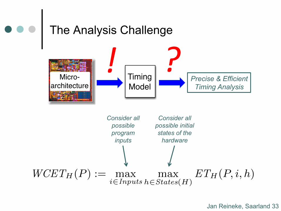
The Analysis Challenge
Precise & Efficient Timing Analysis
Our Vision: PRET Machines
PREcision-Timed processors: Performance & Predicability
+ = PRET
(Image: John Harrison’s H4, first clock to solve longitude problem)
Precision-Timed (PRET) Machines – p. 11/19
Timing Model
Micro-architecture
? !
1. INTRODUCTION
WCETH(P ) := max
i2Inputsmax
h2States(H)ETH(P, i, h)
2. REFERENCES
Consider all possible program inputs
Consider all possible initial states of the
hardware

Jan Reineke, Saarland 34
The Analysis Challenge
1. INTRODUCTION
WCETH(P ) := max
i2Inputsmax
h2States(H)ETH(P, i, h)
2. REFERENCES
Consider all possible program inputs
Consider all possible initial states of the
hardware
Explicitly evaluating ET for all inputs and all hardware states is not feasible in practice: ¢ There are simply too many. è Need for abstraction and thus approximation!

Jan Reineke, Saarland 35
The Analysis Challenge: State of the Art Component Analysis Status
Caches, Branch Target Buffers
Precise & efficient abstractions, for • LRU [Ferdinand, 1999] Not-so-precise but efficient abstractions, for • FIFO, PLRU, MRU [Grund and Reineke,
2008-2011]
Complex Pipelines
Precise but very inefficient; little abstraction Major challenge: timing anomalies
Shared resources, e.g. busses, shared caches, DRAM
No realistic approaches yet Major challenge: interference between hardware threads à execution time depends on corunning tasks

Jan Reineke, Saarland 36
A
A
Resource 1
Resource 2
Resource 1
Resource 2
C
B C
B
D E
D E
Scheduling Anomaly
Timing Anomalies
Timing Anomaly = Local worst-case does not imply Global worst-case

Jan Reineke, Saarland 37
Timing Anomalies
Timing Anomaly = Local worst-case does not imply Global worst-case
A
A
Cache Miss
Cache Hit
C
Branch Condition Evaluated
Prefetch B - Miss C
Speculation Anomaly

Jan Reineke, Saarland 38
The Design Challenge
Wanted: Multi-/many-core architecture with ¢ No timing anomalies à precise & efficient analysis of individual cores ¢ Temporal isolation between cores à independent/incremental development & analysis
and high performance!

Jan Reineke, Saarland 39
Approaches to the Design Challenge
At the level of individual cores: ¢ Simple in-order pipelines, with static or no
branch prediction ¢ Scratchpad Memories or LRU Caches
Software-controlled
caches

Jan Reineke, Saarland 40
Approaches to the Design Challenge
For resources shared among multiple cores: ¢ Temporal partitioning, e.g.
l TDMA arbitration of buses, shared memories l Thread-interleaved pipeline in PRET
¢ Spatial partitioning, e.g. l Partition shared caches l Partition shared DRAM
à Temporal isolation

Jan Reineke, Saarland 41
Design Challenge: Predictable Pipelining
from Hennessy and Patterson, Computer Architecture: A Quantitative Approach, 2007.
Pipeline It!
Hennessey and Patterson, Computer Architecture: A Quantitative Approach, 2007.

Jan Reineke, Saarland 42
Pipelining: Hazards
from Hennessy and Patterson, Computer Architecture: A Quantitative Approach, 2007.
Great Except for Hazards
Hennessey and Patterson, Computer Architecture: A Quantitative Approach, 2007.

Jan Reineke, Saarland 43
Forwarding helps, but not all the time… ...But It Does Not Solve Everything...
LD R1, 45(r2)
DADD R5, R1, R7
BE R5, R3, R0
ST R5, 48(R2)
Unpipelined F D E M W F D E M W F D E M W F D E M W
F D E M W
The Dream F D E M W
F D E M W
F D E M W
F D E M W
The Reality F D E M W Memory Hazard
F D E M W Data Hazard
F D E M W Branch Hazard

Jan Reineke, Saarland 44
Solution: PTARM Thread-interleaved Pipelines [Lickly et al., CASES 2008]
Our Solution: Thread-Interleaved Pipelines
+
An old idea from the 1960s
T1: F D E M W F D E M W
T2: F D E M W F D E M W
T3: F D E M W F D E M W
T4: F D E M W F D E M W
T5: F D E M W F D E M W
But what about memory?
Lee and Messerschmitt,Pipeline InterleavedProgrammable DSPs,ASSP-35(9), 1987.
Our Solution: Thread-Interleaved Pipelines
+
An old idea from the 1960s
T1: F D E M W F D E M W
T2: F D E M W F D E M W
T3: F D E M W F D E M W
T4: F D E M W F D E M W
T5: F D E M W F D E M W
But what about memory?
Lee and Messerschmitt,Pipeline InterleavedProgrammable DSPs,ASSP-35(9), 1987.
Each thread occupies only one stage of the pipeline at a time à No hazards; perfect utilization of pipeline à Simple hardware implementation (no forwarding, etc.) à Each instruction takes the same amount of time à Temporal isolation between different hardware threads Drawback: reduced single-thread performance

Jan Reineke, Saarland 45
Design Challenge: DRAM Controller
Translates sequences of memory accesses by Clients (CPUs and I/O) into legal sequences of DRAM commands
l Needs to obey all timing constraints l Needs to insert refresh commands sufficiently often l Needs to translate “physical” memory addresses into row/column/
bank tuples
CPU1
CPU1
I/O
...
DRAM Module
Interconnect + Arbitration
Memory Controller

Jan Reineke, Saarland 46
Dynamic RAM Timing Constraints
DIMMaddr+cmd
chip select 0
16
data
chip select 1
x16
Device
16
data
16
data
16
data
x16
Device
x16
Device
x16
Device
x16
Device
x16
Device
x16
Device
x16
Device
64
data
Rank 0 Rank 1
address
I/O
Re
gis
ters
+
Da
ta I
/OAddress Register
Control
Logic
Mode Register
16
data
command
chip select
DRAM Device
BankBankBankBankRow
Address Mux
RefreshCounter
I/O Gating
DRAM Array
Row
Decoder
Sense Amplifiers
and Row Buffer
Column Decoder/Multiplexer
Ro
w
Ad
dre
ss
Bank
CapacitorBit line
Word line
Transistor
Capacitor
DRAM Memory Controllers have to conform to different timing constraints that define minimal distances between consecutive DRAM commands. Almost all of these constraints are due to the sharing of resources at different levels of the hierarchy:
Needs to insert refresh commands sufficiently often
Rows within a bank share sense amplifiers
Banks within a DRAM device share I/O gating and control logic
Different ranks share data/address/command busses

Jan Reineke, Saarland 47
General-Purpose DRAM Controllers
¢ Schedule DRAM commands dynamically ¢ Timing hard to predict even for single client:
l Timing of request depends on past requests: • Request to same/different bank? • Request to open/closed row within bank? • Controller might reorder requests to minimize latency
l Controllers dynamically schedule refreshes ¢ No temporal isolation. Timing depends on
behavior of other clients: l They influence sequence of “past requests” l Arbitration may or may not provide guarantees

Jan Reineke, Saarland 48
Thread 2
Thread 1
General-Purpose DRAM Controllers
Load B1.R3.C2
Load B2.R4.C3
Store B4.R3.C5
Arbitration
Memory Controller
Load B3.R3.C2
Load B3.R5.C3
Store B2.R3.C5
?Load B1.R3.C2
Load B3.R3.C2
Load B2.R4.C3
Store B4.R3.C5
Load B3.R5.C3
Store B2.R3.C5

Jan Reineke, Saarland 49
Thread 2
Thread 1
General-Purpose DRAM Controllers
Load B1.R3.C2
Load B2.R4.C3
Store B4.R3.C5
Arbitration
Memory Controller
Load B3.R3.C2
Load B3.R5.C3
Store B2.R3.C5
?Load B1.R3.C2
Load B3.R3.C2
Load B2.R4.C3
Store B4.R3.C5
Load B3.R5.C3
Store B2.R3.C5

Jan Reineke, Saarland 50
General-Purpose DRAM Controllers
Load B1.R3.C2
Load B1.R4.C3
Load B1.R3.C5 …
RAS B1.R3
CAS B1.C2
… RAS B1.R4
CAS B1.C3
… RAS B1.R3
CAS B1.C5
…
RAS B1.R3
CAS B1.C2
… RAS B1.R4
CAS B1.C3
… CAS B1.C5
Memory Controller
?

Jan Reineke, Saarland 51
PRET DRAM Controller: Three Innovations [Reineke et al., CODES+ISSS 2011]
¢ Expose internal structure of DRAM devices: l Expose individual banks within DRAM device as
multiple independent resources
¢ Defer refreshes to the end of transactions l Allows to hide refresh latency
¢ Perform refreshes “manually”: l Replace standard refresh command with multiple reads
CPU1
CPU1
I/O
...
Interconnect
+ Arbitration
PRET DRAM
Controller DRAM
Module
DRAM
Module
DRAM
Module
DRAM
Bank

Jan Reineke, Saarland 52
PRET DRAM Controller: Exploiting Internal Structure of DRAM Module
l Consists of 4-8 banks in 1-2 ranks • Share only command and data bus, otherwise independent
l Partition banks into four groups in alternating ranks l Cycle through groups in a time-triggered fashion
Bank 0
Bank 1
Bank 2
Bank 3
Rank 0:
Bank 0
Bank 1
Bank 2
Bank 3
Rank 1:

Jan Reineke, Saarland 53
PRET DRAM Controller: Exploiting Internal Structure of DRAM Module
l Consists of 4-8 banks in 1-2 ranks • Share only command and data bus, otherwise independent
l Partition banks into four groups in alternating ranks l Cycle through groups in a time-triggered fashion
Bank 0
Bank 1
Bank 2
Bank 3
Rank 0:
Bank 0
Bank 1
Bank 2
Bank 3
Rank 1:
• Successive accesses to same group obey timing constraints • Reads/writes to different groups do not interfere

Jan Reineke, Saarland 54
PRET DRAM Controller: Exploiting Internal Structure of DRAM Module
l Consists of 4-8 banks in 1-2 ranks • Share only command and data bus, otherwise independent
l Partition banks into four groups in alternating ranks l Cycle through groups in a time-triggered fashion
Bank 0
Bank 1
Bank 2
Bank 3
Rank 0:
Bank 0
Bank 1
Bank 2
Bank 3
Rank 1:
• Successive accesses to same group obey timing constraints • Reads/writes to different groups do not interfere
Provides four independent and predictable resources

Jan Reineke, Saarland 55
Conventional DRAM Controller (DRAMSim2) vs PRET DRAM Controller: Latency Evaluation
256 512 768 1,024 1,280 1,536 1,792 2,0480
200
400
600
800 Benefit of burst length 8 over burst length 4
size of transfer [bytes]
late
ncy
[cyc
les]
Shared Predator, BL = 4, accounting for all refreshesDLr(x): PRET, BL = 4, accounting for all refreshesShared Predator, BL = 8, accounting for all refreshesDLr(x): PRET, BL = 8, accounting for all refreshes
Figure 8: Latencies of Predator and PRET for request sizes upto 2KB under burst lengths 4 and 8.
5.4 BandwidthWe describe the peak bandwidth achieved by the PRET DRAM
controller. In the case of the burst length being 4, disregardingrefreshes, we send out four CAS commands every 13 cycles. EachCAS results in a transfer of a burst of size 8 ·4 = 32 bytes over theperiod of two cycles5. The memory controller and the data bus arerunning at a frequency of 200 MHz. So, disregarding refreshes thecontroller would provide a bandwidth of 200 MHz· 4
13 · 32 bytes ⇥1.969GB/s. We issue a refresh command in every 60th slot. Thisreduces the available bandwidth to 59
60 · 1.969GB/s ⇥ 1.936GB/s,which are 60.5% of the data bus bandwidth.
For burst length 8, we transfer 8 · 8 = 64 bytes every five cyclesand perform a refresh in every 39th slot, resulting in an availablebandwidth of 200MHz · 38
39 ·15 · 64 bytes ⇥ 2.494GB/s, or 77.95%
of the data bus bandwidth.
6. EXPERIMENTAL EVALUATIONWe present experimental results to verify that the design of the
PRET DRAM controller honors the derived analytical bounds. Wehave implemented the PRET DRAM controller, and compare itvia simulation with a conventional DRAM controller. We use thePTARM simulator6 and extend it to interface with both memorycontrollers to run synthetic benchmarks that simulate memory ac-tivity. The PTARM simulator is a C++ simulator that simulatesthe PRET architecture with four hardware threads running througha thread-interleaved pipeline. We use a C++ wrapper around theDRAMSim2 simulator [17] to simulate memory access latenciesfrom a conventional DRAM controller. A first-come, first-servedqueuing scheme is used to queue up memory requests to the DRAM-Sim2 simulator. The PRET DRAM controller was also written inC++ based on the description in Section 4. The benchmarks we useare all written in C, and compiled using the GNU ARM cross com-piler. The DMA transfer latencies that are measured begin whenthe DMA unit issues its first request and end when the last requestfrom the DMA unit is completed.
6.1 Experimental ResultsWe setup our experiment to show the effects of interference on
memory access latency for both memory controllers. We first setupour main thread to run different programs that initiate fixed-size
5In double-data rate (DDR) memory two transfers are performedper clock cycle.6The PTARM simulator is available for download at http://chess.eecs.berkeley.edu/pret/release/ptarm.
0 0.5 1 1.5 2 2.5 30
1,000
2,000
3,000
Interference [# of other threads occupied]
late
ncy
[cyc
les]
4096B transfers, conventional controller4096B transfers, PRET controller
1024B transfers, conventional controller1024B transfers, PRET controller
Figure 9: Latencies of conventional and PRET memory con-troller with varying interference from other threads.
DMA transfers (256, 512, 1024, 2048 and 4096 bytes) at randomintervals. The DMA latencies of the main thread is what is mea-sured and shown in Figure 9 and Figure 10. To introduce interfer-ence within the system, we run a combination of two programs onthe other hardware threads in PTARM simulator. The first programcontinuously issues DMA requests of large size (4096 bytes) in or-der to fully utilize the memory bandwidth. The second programutilizes half the memory bandwidth by issuing DMA requests ofsize 4096 bytes half as frequently as the first program. In Figure 9,we define thread occupancy on the x-axis as the memory bandwidthoccupied by the combination of all threads. 0.5 means we have onethread running the second program along side the main thread. 1.0means we have one thread running the first program along side themain thread. 1.5 means we have one thread running the first pro-gram, one thread running the second program, and both threads arerunning along side the main thread, and so on. 3 is the maximumwe can achieve because the PTARM simulator has a total of fourhardware threads (the main thread occupies one of the four). Wemeasured the latency of each fixed size transfer for the main threadto observe the transfer latency in the presence of interference frommemory requests by other threads.
In Figure 9, we show measurements taken from two differentDMA transfer sizes, 1024 and 4096 bytes. The marks in the figureshow the average latency measured over 1000 iterations. The errorbars above and below the marks show the worst-case and best-caselatencies of each transfer size over the same 1000 iterations. In bothcases, without any interference, the conventional DRAM controllerprovides better access latencies. This is because without any inter-ference, the conventional DRAM controller can often exploit rowlocality and service requests immediately. The PRET DRAM con-troller on the other hand uses the periodic pipelined access scheme,thus even though no other threads are accessing memory, the mem-ory requests still need to wait for their slot to get access to theDRAM. However, as interference is gradually introduced, we ob-serve increases in latency for the conventional DRAM controller.This could be caused by the first-come, first-served buffer, or bythe internal queueing and handling of requests by DRAMSim2.The PRET DRAM controller however is unaffected by the inter-ference created by the other threads. In fact, the latency valuesthat were measured from the PRET DRAM controller remain the
0 1,000 2,000 3,000 4,000
0
1,000
2,000
3,000
transfer size [bytes]
aver
age
late
ncy
[cyc
les]
Conventional controllerPRET controller
Figure 10: Latencies of conventional and PRET memory con-troller with maximum load by interfering threads and varyingtransfer size.
same under all different thread occupancies. This demonstrates thetemporal isolation achieved by the PRET DRAM controller. Anytiming analysis on the memory latency for one thread only needsto be done in the context of that thread. We also see the range ofmemory latencies for the conventional DRAM controller increaseas the interference increases. But the range of access latencies forthe PRET DRAM controller not only remains the same through-out, but is almost negligible for both transfer sizes7. This shows thepredictable nature of the PRET DRAM controller.
In Figure 10 we show the memory latencies under full load (threadoccupancy of 3) for different transfer sizes. This figure shows thatunder maximum interference from the other hardware threads, thePRET DRAM controller is less affected by interference even astransfer sizes increase. More importantly, when we compare thenumbers from Figure 10 to Figure 8, we confirm that the theoret-ical bandwidth calculations hold even under maximum bandwidthstress from the other threads.
7. CONCLUSIONS AND FUTURE WORKIn this paper we presented a DRAM controller design that is
predictable with significantly reduced worst-case access latencies.Our approach views the DRAM device as multiple independent re-sources that are accessed in a periodic pipelined fashion. This elim-inates contention for shared resources within the device to providetemporally predictable and isolated memory access latencies. Werefresh the DRAM through row accesses instead of standard re-freshes. This results in improved worst-case access latency at aslight loss of bandwidth. Latency bounds for our memory con-troller, determined analytically and confirmed through simulation,show that our controller is both timing predictable and providestemporal isolation for memory accesses from different resources.
Thought-provoking challenges remain in the development of anefficient, yet predictable memory hierarchy. In conventional multi-core architectures, local memories such as caches or scratchpadsare private, while access to the DRAM is shared. However, inthe thread-interleaved PTARM, the instruction and data scratchpadmemories are shared, while access to the DRAM is not. We havedemonstrated the advantages of privatizing parts of the DRAM forworst-case latency. It will be interesting to explore the consequencesof the inverted sharing structure on the programming model.
We envision adding instructions to the PTARM that allow threadsto pass ownership of DRAM resources to other threads. This would,
7The range (worst-case latency - best-case latency) was approxi-mately 90ns for 4096 bytes transfers and approximately 20ns for1024 byte transfers.
for instance, allow for extremely efficient double-buffering imple-mentations. We also plan to develop new scratchpad allocationtechniques, which use the PTARM’s DMA units to hide memorylatencies, and which take into account the transfer-size dependentlatency bounds derived in this paper.
8. REFERENCES[1] B. Akesson, K. Goossens, and M. Ringhofer, “Predator: a
predictable SDRAM memory controller,” in CODES+ISSS.ACM, 2007, pp. 251–256.
[2] B. Akesson, “Predictable and composable system-on-chipmemory controllers,” Ph.D. dissertation, EindhovenUniversity of Technology, Feb. 2010.
[3] M. Paolieri, E. Quiñones, F. Cazorla, and M. Valero, “Ananalyzable memory controller for hard real-time CMPs,”IEEE Embedded Systems Letters, vol. 1, no. 4, pp. 86–90,2010.
[4] I. Liu, J. Reineke, and E. A. Lee, “A PRET architecturesupporting concurrent programs with composable timingproperties,” in 44th Asilomar Conference on Signals,Systems, and Computers, November 2010.
[5] S. A. Edwards and E. A. Lee, “The case for the precisiontimed (PRET) machine,” in DAC. New York, NY, USA:ACM, 2007, pp. 264–265.
[6] D. Bui, E. A. Lee, I. Liu, H. D. Patel, and J. Reineke,“Temporal isolation on multiprocessing architectures,” inDAC. ACM, June 2011.
[7] B. Jacob, S. W. Ng, and D. T. Wang, Memory Systems:Cache, DRAM, Disk. Morgan Kaufmann Publishers,September 2007.
[8] JEDEC, DDR2 SDRAM SPECIFICATION JESD79-2E.,2008.
[9] B. Akesson, L. Steffens, E. Strooisma, and K. Goossens,“Real-time scheduling using credit-controlled static-priorityarbitration,” in RTCSA, Aug. 2008, pp. 3 –14.
[10] B. Bhat and F. Mueller, “Making DRAM refreshpredictable,” in ECRTS, 2010, pp. 145–154.
[11] P. Atanassov and P. Puschner, “Impact of DRAM refresh onthe execution time of real-time tasks,” in Proc. IEEEInternational Workshop on Application of ReliableComputing and Communication, Dec. 2001, pp. 29–34.
[12] R. Wilhelm et al., “Memory hierarchies, pipelines, and busesfor future architectures in time-critical embedded systems,”IEEE TCAD, vol. 28, no. 7, pp. 966–978, 2009.
[13] R. Bourgade, C. Ballabriga, H. Cassé, C. Rochange, andP. Sainrat, “Accurate analysis of memory latencies forWCET estimation,” in RTNS, Oct. 2008.
[14] T. Ungerer et al., “MERASA: Multi-core execution of hardreal-time applications supporting analysability,” IEEE Micro,vol. 99, 2010.
[15] M. Schoeberl, “A java processor architecture for embeddedreal-time systems,” Journal of Systems Architecture, vol. 54,no. 1-2, pp. 265 – 286, 2008.
[16] A. Hansson, K. Goossens, M. Bekooij, and J. Huisken,“CoMPSoC: A template for composable and predictablemulti-processor system on chips,” ACM TODAES, vol. 14,no. 1, pp. 1–24, 2009.
[17] P. Rosenfeld, E. Cooper-Balis, and B. Jacob, “DRAMSim2:A cycle accurate memory system simulator,” ComputerArchitecture Letters, vol. 10, no. 1, pp. 16 –19, Jan. 2011.
Varying interference for fixed transfer size:
Varying transfer size at maximal interference:
More information: http://chess.eecs.berkeley.edu/pret/

Jan Reineke, Saarland 56
Emerging Challenge: Microarchitecture Selection & Configuration
Embedded Software
Timing Requirements
with ? Family of Microarchitectures
= Platform

Jan Reineke, Saarland 57
Emerging Challenge: Microarchitecture Selection & Configuration
Embedded Software
Timing Requirements
with ? Family of Microarchitectures
= Platform
Choices: • Processor frequency • Sizes and latencies
of local memories • Latency and
bandwidth of interconnect
• Presence of floating-point unit
• …

Jan Reineke, Saarland 58
Emerging Challenge: Microarchitecture Selection & Configuration
Embedded Software
Timing Requirements
with ? Family of Microarchitectures
= Platform
Choices: • Processor frequency • Sizes and latencies
of local memories • Latency and
bandwidth of interconnect
• Presence of floating-point unit
• …
Select a microarchitecture that a) satisfies all timing requirements, and b) minimizes cost/size/energy.

Jan Reineke, Saarland 59
Conclusions
Challenges in modeling analysis design remain.

Jan Reineke, Saarland 60
Conclusions
Challenges in modeling analysis design remain.
Progress based on automation abstraction partitioning
has been made.

Jan Reineke, Saarland 61
Conclusions
Challenges in modeling analysis design remain.
Progress based on automation abstraction partitioning
has been made.
Thank you for your attention!