Embed Size (px)
Citation preview

CH.6 Random Sampling andDescriptive Statistics
• Population vs Sample• Random sampling• Numerical summaries :
– sample mean, sample variance, sample range• Stem-and-Leaf Diagrams
– Median, quartiles, percentiles, mode, interquartile range (IQR)• Frequency distributions and histograms• Box plots
– Whisker, outlier• Time-sequence plots• Probability plots

Population
• The collection of things (parts, people, services) -- called “members” -- under study
• The letter N is usually defined to be the number of members in the population
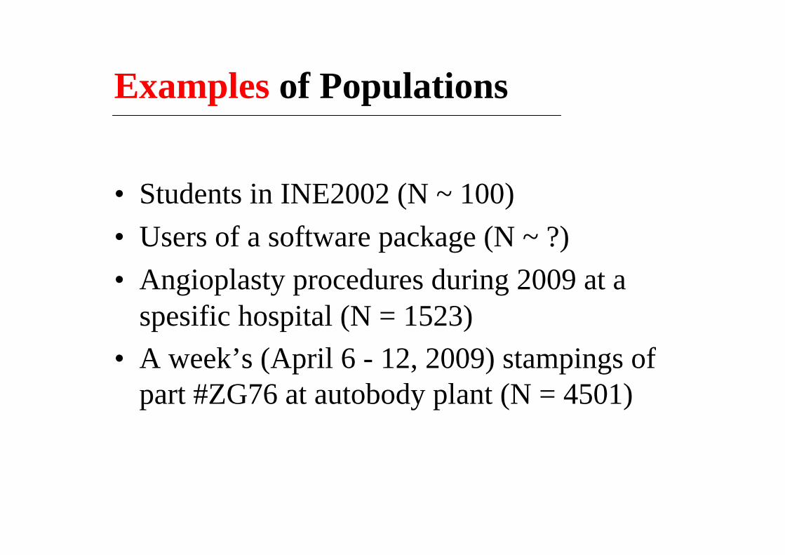
Examples of Populations
• Students in INE2002 (N ~ 100)• Users of a software package (N ~ ?)• Angioplasty procedures during 2009 at a
spesific hospital (N = 1523)• A week’s (April 6 - 12, 2009) stampings of
part #ZG76 at autobody plant (N = 4501)

Sample• Measurement of only a subset of the
population . These will be used to say something about the variables of the entire population.
• The letter n (the “sample size”) is usually used to represent the number of items in in this subset

Examples of Samples• Asking only 20 (out of 100) INE2002
students the current value of their GPA’s• Surveying only some of a software package’s
users • Getting detailed angioplasty data only for
procedures done on Mondays• Measuring one auto panel out of every 100
produced

Why Use Samples?• In most situations, it is impossible or impractical to observe
the entire population. • Impractical: it would be time consuming and expensive• Impossible: some (perhaps many) of the members of the
population do not yet exist at the time a decision is to be made,
• Ex: we could not test the tensile strength of all the chassis structural elements
• So generally, we must view the population as conceptual. • Therefore, we depend on a subset of observations from the
population to help make decisions about the population.

Population vs Sample
POPULATION
Sample X1, X2 ,…,Xn
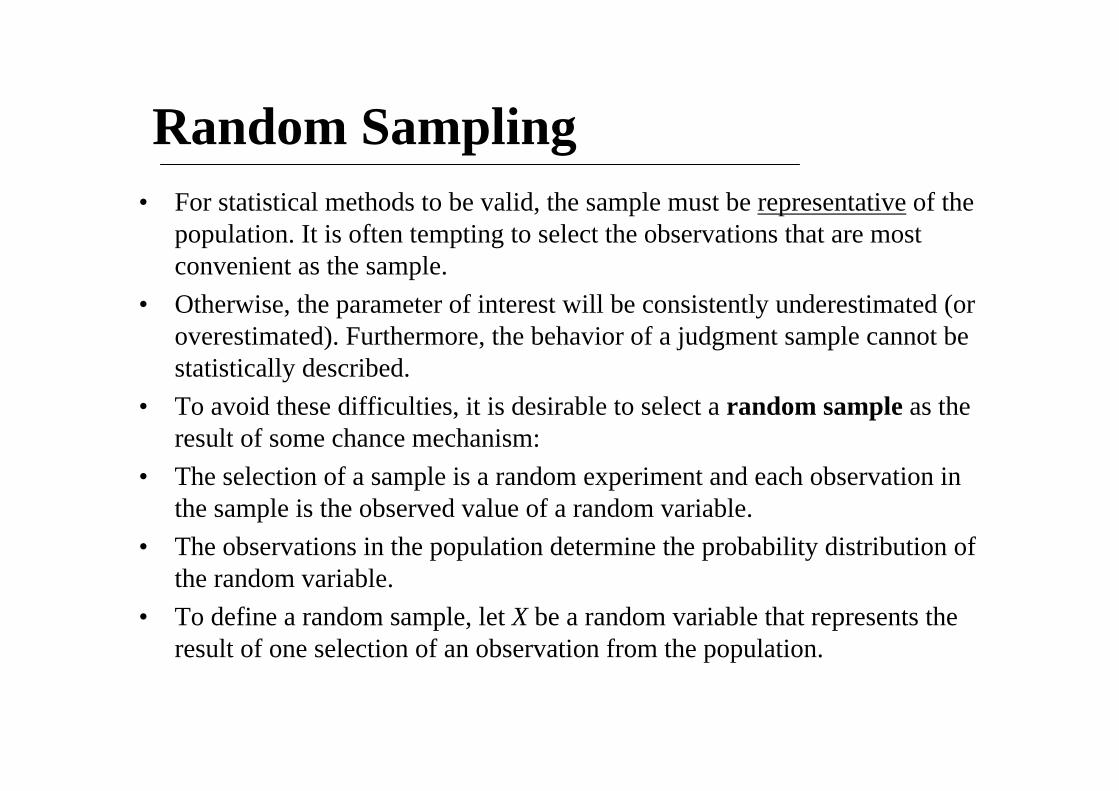
Random Sampling• For statistical methods to be valid, the sample must be representative of the
population. It is often tempting to select the observations that are mostconvenient as the sample.
• Otherwise, the parameter of interest will be consistently underestimated (oroverestimated). Furthermore, the behavior of a judgment sample cannot be statistically described.
• To avoid these difficulties, it is desirable to select a random sample as theresult of some chance mechanism:
• The selection of a sample is a random experiment and each observation in the sample is the observed value of a random variable.
• The observations in the population determine the probability distribution of the random variable.
• To define a random sample, let X be a random variable that represents theresult of one selection of an observation from the population.

Random SamplingThe random variables X1,X2,…,Xn are a random sample of size n if(a) the Xi’s are independent random variables, and(b) every Xi has the same probability distribution.Example:• Suppose, we are investigating the effective service life of an
electronic component used in a cardiac pacemaker (kalp pili) and that component life is normally distributed.
• Then we would expect each of the observations on componentlife in a random sample of n components to be independentrandom variables with exactly the same normal distribution.

6-1 Numerical Summaries
Definition: Sample Mean
Describe data features numericallyEx: characterize the central tendency in the data by arithmetic average which is refered as sample mean
Other examples: sample variance, sample standard deviation, sample range

6-1 Numerical Summaries
Example 6-1

6-1 Numerical Summaries
The sample mean as a balance point for a system of weights.

6-1 Numerical Summaries
Population Mean
For a finite population with N measurements, the mean is
The sample mean is a reasonable estimate of the population mean.

6-1 Numerical Summaries
Definition: Sample Variance

6-1 Numerical Summaries
How does the Sample Variance Measure Variabilitythrough the deviations ?xxi −

6-1 Numerical Summaries
Example 6-2
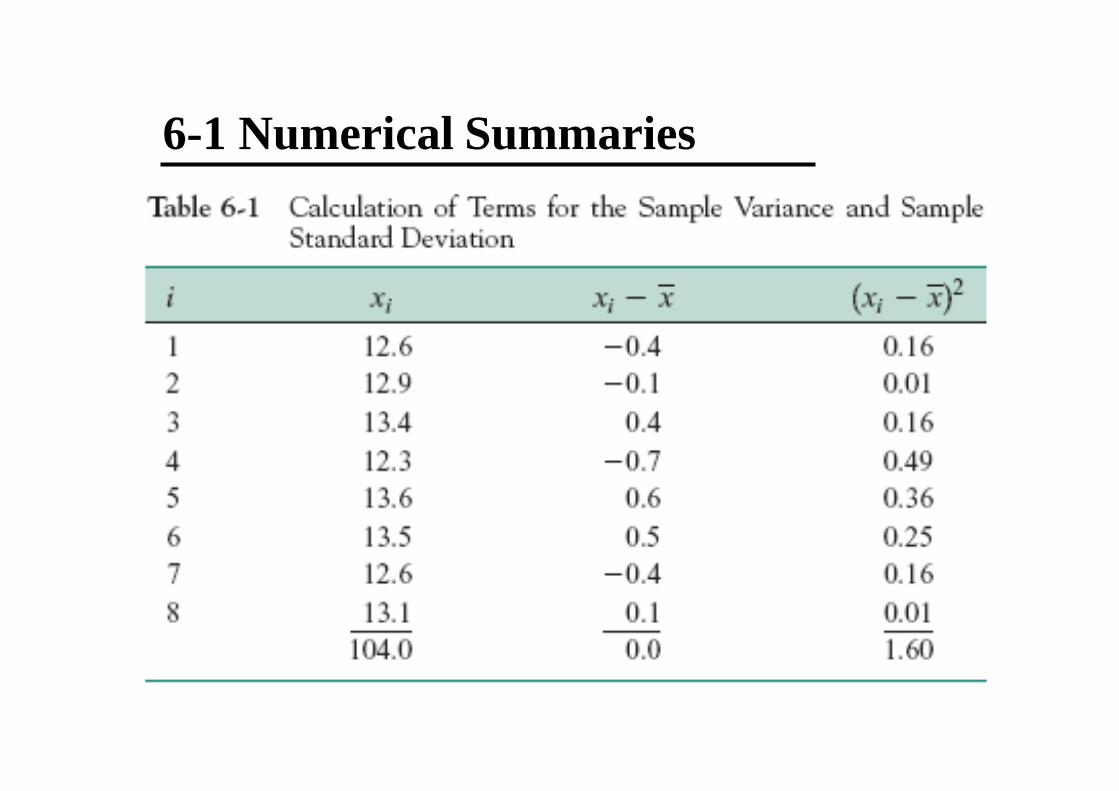
6-1 Numerical Summaries

6-1 Numerical Summaries
2
12 2 2
2 1 1
1 1
n
in ni
i ii i
xx nx x
nsn n
=
= =
⎛ ⎞⎜ ⎟⎝ ⎠− −
= =− −
∑∑ ∑
Computation of s2
Shortcut methodto compute s
( ) 11 n
iix n x
== ∑
Remember
( )2 2 2 2 2
2 1 1 1 1
2 2 2 2 2
1 1
( ) 2 2
1 1 1
2 2
1 1
n n n n
i i i i ii i i i
n n
i ii i
x x x x xx x nx x xs
n n n
x nx xnx x nx nx
n n
= = = =
= =
− + − + −= = =
− − −
+ − + −= =
− −
∑ ∑ ∑ ∑
∑ ∑

6-1 Numerical Summaries
Population Variance
When the population is finite and consists of N values, we may define the population variance as
The sample variance is a reasonable estimate of the population variance.

6-1 Numerical Summaries
Definition

6-2 Stem-and-Leaf Diagrams
Steps for Constructing a Stem-and-Leaf Diagram

6-2 Stem-and-Leaf Diagrams
psi: pounds per square inch
min
max

6-2 Stem-and-Leaf Diagrams
From the diagram• Most of the data lie
between 110 and 200 psi• A central value is
somewhere between 150 and 160 psi
• The data are distributedapproximatelysymmetrically about thecentral value
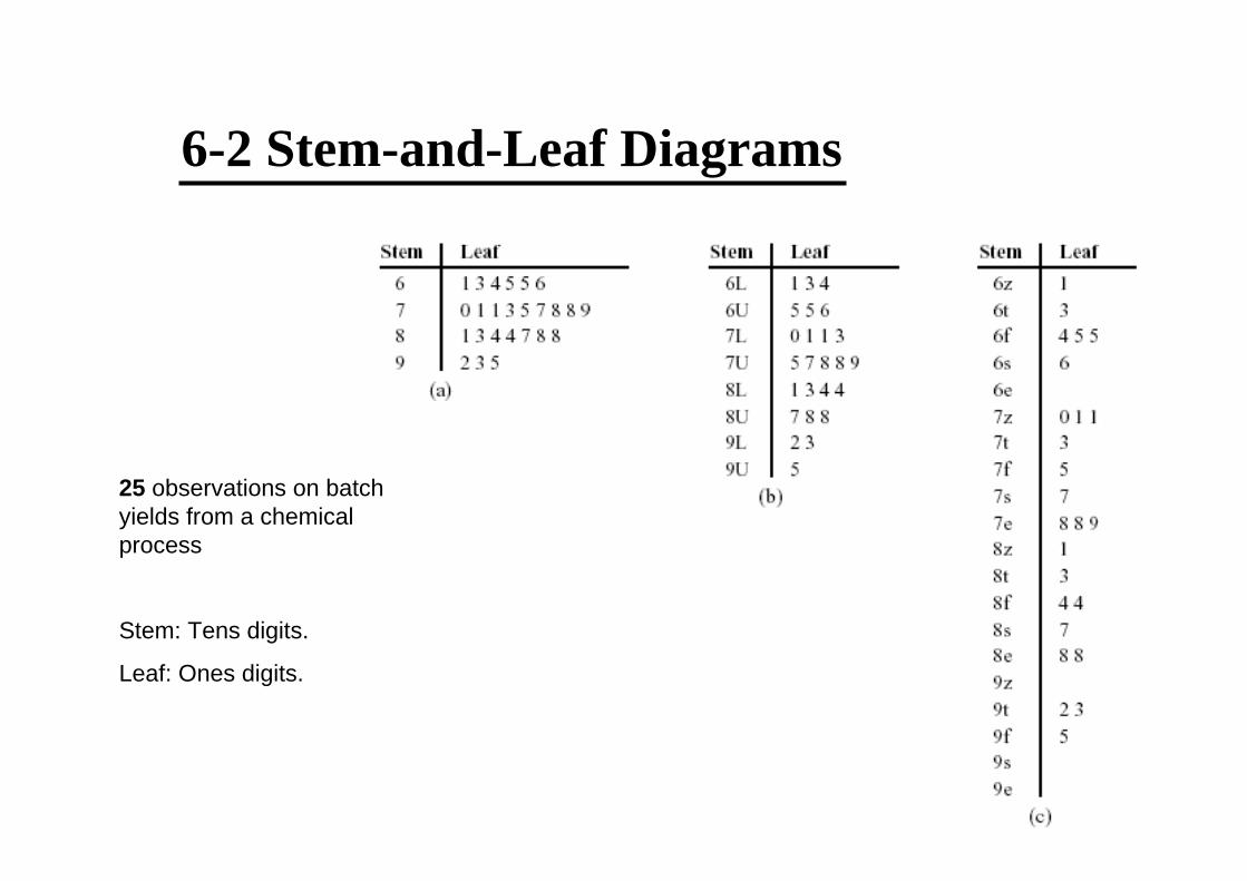
6-2 Stem-and-Leaf Diagrams
25 observations on batchyields from a chemicalprocess
Stem: Tens digits.
Leaf: Ones digits.

6-2 Stem-and-Leaf Diagrams - ordered
Easier to find
• percentiles
• quartiles
• median

Data Features : median, range, quartiles
The median, , is a measure of central tendency that divides the data into two equal parts, half below the median and half above. If the number of observations is even, the median is halfway between the two central values.
In the 80 compressive strength data, the 40th and 41st values of strength are 160 and 163. So the median is (160 + 163)/2 = 161.5. If the number of observations is odd, the median is the central value.
The range is a measure of variability that can be easily computed from the ordered stem-and-leaf display. It is the maximum minus the minimum measurement. From the figure, the range is 245 - 76 = 169.
6-2 Stem-and-Leaf Diagrams
x

Data Features : median, range, quartiles, interquartile range, mode
When an ordered set of data is divided into four equal parts, the division points are called quartiles.
The first or lower quartile, q1 , is a value that has approximately one-fourth (25%) of the observations below it and approximately 75% of the observations above.
The second quartile, q2, has approximately one-half (50%) of the observations below its value. The second quartile is exactly equal to the median.
The third or upper quartile, q3, has approximately three-fourths (75%) of the observations below its value. As in the case of the median, the quartiles may not be unique.
6-2 Stem-and-Leaf Diagrams

Data Features : median, range, quartiles, interquartile range, mode
• The compressive strength data contains n = 80 observations. Thefirst and third quartiles (q1 and q3) are calculated as the
(n + 1)/4 and 3(n + 1)/4 ordered observations and interpolated as needed.
• For example, (80 + 1)/4 = 20.25 and 3(80 + 1)/4 = 60.75.
• q1 is interpolated between the 20th and 21st ordered observationq1 = [(145-143)/(21-20)]*(20.25-20)+143 = 143.50
• q3 is interpolated between the 60th and 61st ordered observationq3 = [(181-181)/(61-60)]*(60.75-60)+181 = 181.00
6-2 Stem-and-Leaf Diagrams

Data Features : median, range, quartiles, interquartile range, mode
• The interquartile range is the difference between the upper and lower quartiles, and it is sometimes used as a measure of variability.IQR=q3 – q1= 181-143.5 = 37.5
• In general, the 100kth percentile is a data value such that approximately 100k% of the observations are at or below this value and approximately 100(1 - k)% of them are above it.
•The sample mode is the most frequently occuring data value.Mode is 158 in the compressive strength data.
6-2 Stem-and-Leaf Diagrams

Stem-and-Leaf Exercise 6.15 (6.23)
164216089101269375845865
1750133011201315122310151020
15121764194020238851270798
146810551820159478512031085
990156010002100221518831315
123814161792189070615671258
150175815221452160514811502
1750157817821018110211091540
1781110218881910101614211310
1535173012602265167421301115
70 data: Numbers of cycles to failure of aluminum test coupons subjected to repeatedalternating stress at 21000 psi, 18 cycles per second

Stem-and-Leaf Exercise 6.15 (6.23)
• Median = 1436.5
• Q1 = 1097.8
• Q3 = 1735.0

Stem-and-Leaf Exercise 6.16 (6.24)64 data: The percentage of cotton in material used to manufacture men’s shirts
32,736,434,534,933,535,334,133,6
34,337,932,13532,935,13434,7
36,836,832,835,233,636,837,135,1
35,735,135,534,634,736,233,836,3
34,734,134,634,735,935,434,635,6
34,132,537,333,434,63535,434,5
33,633,637,634,233,134,736,633,1
34,634,735,833,832,633,637,834,2

Stem-and-Leaf Exercise 6.16 (6.24)
• Median = 34.7
• Q1 = 33.8
• Q3 = 35.575

6-3 Frequency Distributions and Histograms
• A frequency distribution is a more compact summary of data than a stem-and-leaf diagram.
• To construct a frequency distribution, we must divide the range of the data into intervals, which are usually called class intervals, cells, or bins.
•In practice # bin= where n is the sample size
Constructing a Histogram (Equal Bin Widths):
n

6-3 Frequency Distributions and Histograms
Frequency Distribution of compressive strength for 80 aluminum-lithium alloy specimens.

6-3 Frequency Distributions and Histograms
Histogram of compressive strength for 80 aluminum-lithium alloy specimens.

6-3 Frequency Distributions and Histograms
A histogram of the compressive strength data from Minitab with 17 bins.
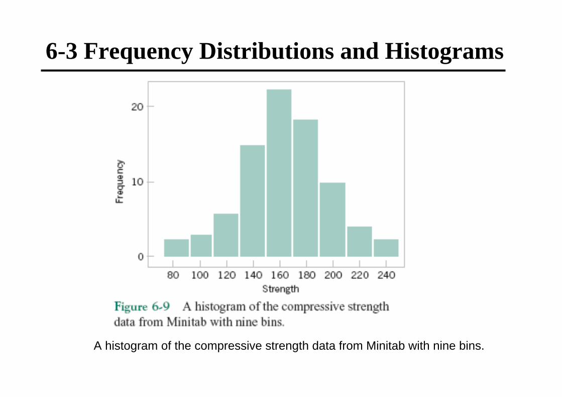
6-3 Frequency Distributions and Histograms
A histogram of the compressive strength data from Minitab with nine bins.

6-3 Frequency Distributions and Histograms
A cumulative distribution plot of the compressive strength data from Minitab.

6-3 Frequency Distributions and Histograms
Histograms for symmetric and skewed distributions.

6-3 Frequency Distributions and Histograms
Histograms for categorical data
Pareto charts can also be used

Exercise 6.32 (6.40)
64 data: The percentage of cotton in material used to manufacture men’s shirts
32,736,434,534,933,535,334,133,6
34,337,932,13532,935,13434,7
36,836,832,835,233,636,837,135,1
35,735,135,534,634,736,233,836,3
34,734,134,634,735,935,434,635,6
34,132,537,333,434,63535,434,5
33,633,637,634,233,134,736,633,1
34,634,735,833,832,633,637,834,2

Frequency Distributions Exercise 6.32 (6.40)
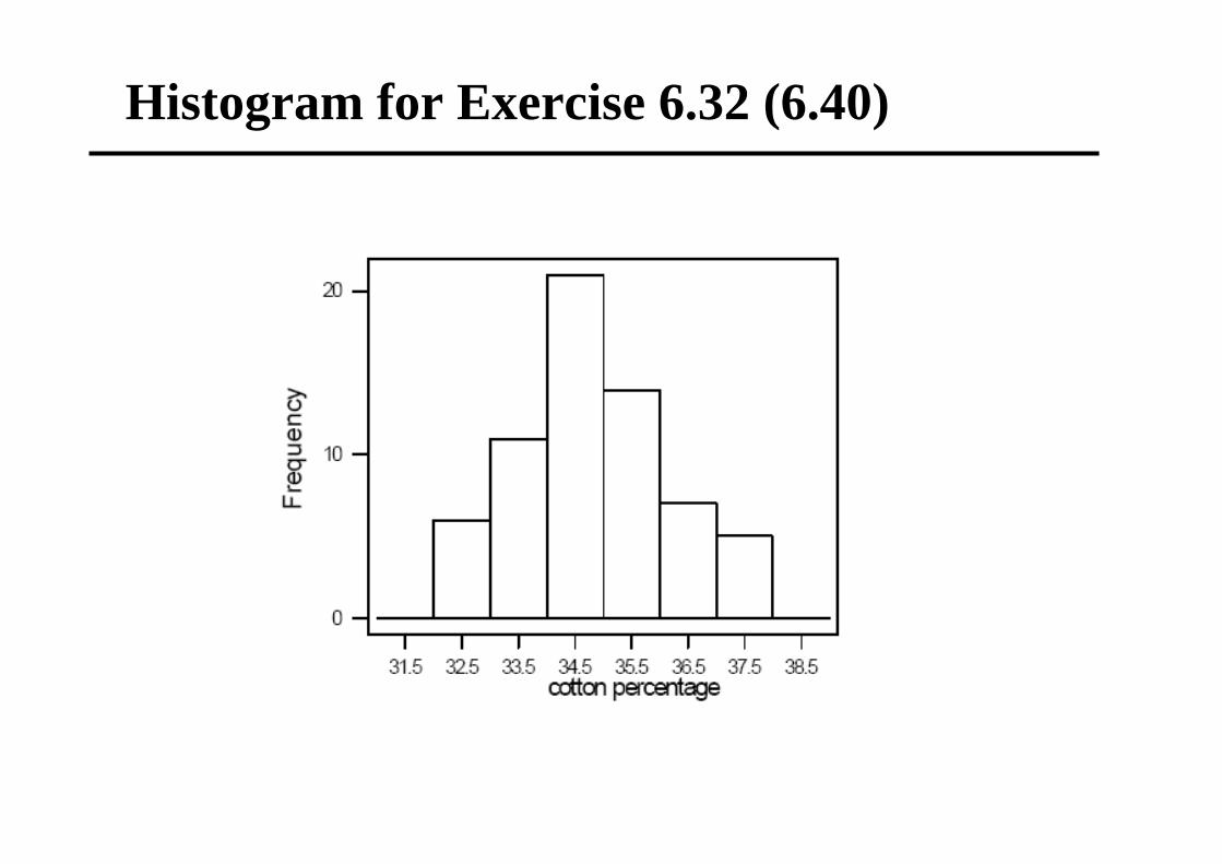
Histogram for Exercise 6.32 (6.40)

6-4 Box Plots
• The box plot is a graphical display that simultaneously describes several important features of a data set, such as center, spread, departure from symmetry, and identification of observations that lie unusually far from the bulk of the data(outliers).
• Whisker• Outlier• Extreme outlier

6-4 Box Plots
Outlier : a point beyond whisker but less than 3 IQR from the box edge
Extreme outlier: a point more than 3 IQR from the box edge

6-4 Box Plots
Box plot for compressive strength data

6-4 Box Plots
Box plots are useful forgraphical comparisonsamong data sets.
Comparative box plots of a quality index at three plants.

6-5 Time Sequence Plots
• A time series or time sequence is a data set in which the observations are recorded in the order in which they occur.
• A time series plot is a graph in which the vertical axis denotes the observed value of the variable (say x) and the horizontal axis denotes the time (which could be minutes, days, years, etc.).
• When measurements are plotted as a time series, weoften see
•trends, •cycles, or •other broad features of the data

6-5 Time Sequence Plots
Company sales by year (a) and by quarter (b).

6-5 Time Sequence Plots
A digidot (stem-and-leaf + time series) plot of the compressive strength data

6-5 Time Sequence Plots
A digidot plot of chemical process concentration readings, observed hourly.
After 20 hours, lower concentrations begin to occur.

6-6 Probability Plots
• Probability plotting is a graphical method for determining whether sample data conform to a hypothesized distribution based on a subjective visual examination of the data.
• Probability plotting typically uses special graph paper, known as probability paper, that has been designed for the hypothesized distribution. Probability paper is widely availablefor the normal, lognormal, Weibull, and various chi-square and gamma distributions.

6-6 Probability Plots Example 6-7

6-6 Probability Plots
Example 6-7 (continued)
• A straight line, chosen subjectively, is drawn through theplotted points.
• In drawing the straight line, you should be influenced moreby the points near the middle of the plot than by theextreme points.
• A good rule of thumb is to draw the line approximatelybetween the 25th and 75th percentile points.
• Imagine a fat pencil lying along the line. If all the pointsare covered by this imaginary pencil, a normal distributionadequately describes the data.

6-6 Probability Plots
Normal probability plot for battery life
obtained fromcumulative frequencies
The points pass the“fat pencil” test, So, the normal distributionis an appropriate model.

6-6 Probability Plots
Normal probability plot obtained from standardized normal scores.
0.5 ( ) ( )j jj P Z z z
n−
= ≤ = Φ

6-6 Probability Plots
Normal probability plots indicating a nonnormal distribution. (a) Light-tailed distribution. (b) Heavy-tailed distribution. (c ) A distribution with positive (or right) skew.

6-6 Excercise 6-71 (6.79)
164216089101269375845865
1750133011201315122310151020
15121764194020238851270798
146810551820159478512031085
990156010002100221518831315
123814161792189070615671258
150175815221452160514811502
1750157817821018110211091540
1781110218881910101614211310
1535173012602265167421301115
70 data: Numbers of cycles to failure of aluminum test coupons subjected to repeatedalternating stress at 21000 psi, 18 cycles per second
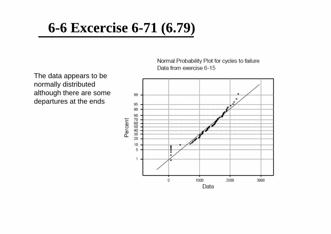
6-6 Excercise 6-71 (6.79)
The data appears to be normally distributedalthough there are somedepartures at the ends

6-6 Excercise 6-27 (6.35)
40 data: Wine gradings on a 0-100 point scale
83909085848889859185
92958987928988919588
90898689929190879390
90919189869191929094

6-6 Excercise 6-27 (6.35)Leaf unit: 0.1Sample mean:
Sample variance:
Sample modes: 90, 91

6-6 Excercise 6-27 (6.35)
1
2
3
1 40 1 10.254 4
2( 1) 40 1 20.54 2
3( 1) 3(40 1) 30.754 4
+ += =
+ += = ===>
+ += =
nfor q
nfor q Median
nfor q
Leaf unit: 0.1Sample quartiles:
1
2
3
8890
91
qq xq
== ==

6-6 Excercise 6-27 (6.35)Leaf unit: 0.1

6-6 Excercise 6-50 (6.58 – data of 6.22)Q1=88.6Q2=90.4Q3=92.2
IQR=3.61.5*IQR=5.4
Whiskers83.496.5
Outliers98.8100.3