Embed Size (px)
Citation preview

1
Ch 13 – Backtracking +
Branch-and-Bound
There are two principal approaches totackling NP-hard problems or other“intractable” problems:
• Use a strategy that guarantees solving theproblem exactly but doesn’t guarantee tofind a solution in polynomial time
• Use an approximation algorithm that canfind an approximate (sub-optimal) solutionin polynomial time
2
Exact solutions
The exact solution approach includes:
• exhaustive search (brute force)
– useful only for small instances
• backtracking
– eliminates some cases from consideration
• branch-and-bound
– further cuts down on the search
– fast solutions for most instances
– worst case is still exponential3
Backtracking : Colouring Example
WA
NT
Q
SA NSW
V
T
R e g
i o n
( V a r i a
b l e )
A s s
i g n m e n
t
A l t e r n a
t i v e s
T
SA
V
WA
NSW
Q
NT
4
Backtracking
• Construct the state space tree:
– nodes: partial solutions
– edges: choices in completing solutions
• Explore the state space tree using depth-first
search
• “Prune” non-promising nodes
– DFS stops exploring subtree rooted at nodes
leading to no solutions and...
– “backtracks” to its parent node
5
Example: n-Queen problem
• Place n queens on an n by n chess
board so that no two of them are on
the same row, column, or diagonal
6
State-space of the four-queens
problem
7
Example: m-coloring problem
• Given a graph and an integer m, color its vertices
using no more than m colors so that no two
adjacent vertices are the same color.
– Run on the following graph with m=3.
c d
a
eb8
Example: Ham Circuit problem
• Given a graph, find one of its Hamiltonian cycles.
– Run on the following graph.
c
d
a
e
b
f
9
Example: Subset-Sum problem
• Find a subset of a given set S = {s1, s2, …, sn}
whose sum is equal to a given integer d.
– Run on S = {3, 5, 6, 7} and d =15.
10
Branch and Bound
• An enhancement of backtracking
• Applicable to optimization problems
• Uses a lower/upper bound for the value of the
objective function for each node (partial solution)
so as to:
– guide the search through state-space
– rule out certain branches as “unpromising”
• Lower bound for minimization problems
• Upper bound for maximization problems
11
Example: The job-employee
assignment problemSelect 1 element in each row of the cost matrix C :
• no 2 selected elements are in the same col;
• and the sum is minimized
For example:
Job 1Job 2Job 3Job 4
Person a 9 2 7 8
Person b 6 4 3 7
Person c 5 8 1 8
Person d 7 6 9 4
Lower bound: Any solution to this problem will have
total cost of at least: 2 + 3 + 1 + 4 = 10. 12
Assignment problem: lower bounds
Job 1 Job 2 Job 3 Job 4
Person a 9 2 7 8
Person b 6 4 3 7
Person c 5 8 1 8
Person d 7 6 9 4
Lower bound: same formula, but remove the selected col.
13
Complete state-space
9 2 7 8
6 4 3 7
5 8 1 8
7 6 9 4
14
Knapsack problem
• Run BB algorithm on the following data:
– W = 10 (max weight)
– Elements (weight, benefit):
(4,40), (7,42), (5,25), (3,12)
• Upper bound is calculated as
– ub = v + (W-w)(vi+1/wi+1)
• v = value of already selected items
• w = weight of already selected items
15
Knapsack problem
(4,40, 10),
(7,42, 6),
(5,25, 5),
(3,12, 4)
W = 10
16
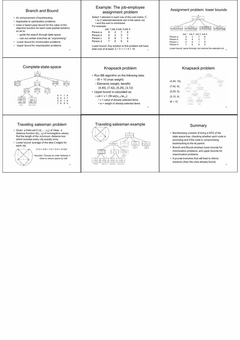
Traveling salesman problem
• Given a finite set C={c1,...,cm} of cities, a
distance function d(ci, c j) of nonnegative values,
find the length of the minimum distance tour
which includes every city exactly once.
• Lower bound: average of the best 2 edges for
each city
(1+3 + 3+6 + 1+2 + 3+4 + 2+3)/2
Heuristic: Choose an order between 2
cities to reduce space by half.
17
Traveling salesman example
18
Summary
• Backtracking consists of doing a DFS of the
state space tree, checking whether each node is
promising and if the node is nonpromising
backtracking to the its parent.
• Branch and Bound employs lower bounds for
minimization problems, and upper bounds for
maximization problems.
• It prunes branches that will lead to inferior
solutions (than the ones already found).