Embed Size (px)
Citation preview

Ch t 10Chapter 10
Frequency ResponseFrequency Response Techniques
Representation of complex number
Introduction
MjBA
jMe
)/(tan 1 AB22 BAM
Im
where
ijh
&
jMe
1)(sin)(cos 22 xxB
M
s-plane sincos je j where
A point on the unit circleMagnitude: 1)(sin)(cos xx
cossintan 1Re
A
M
Note Euler’s formula:
g
Phase:
ee
eex
jxjx
jxjx
i
2cos
Note. Euler s formula:
jx
2sin
Any transfer function G(s)
)()( sNG js )()( jNjG
)())(()()(
21 npspspssG
j)())((
)()(21
MjBA
jpjpjpjNjG
n
complex!
)()(
jGjGM
Any transfer function can be represented as magnitude and phase angle

Frequency response: steady-state response of a linear system to a sinusoidal input
A. The Concept of Frequency Response
Frequency response: steady state response of a linear system to a sinusoidal input
js 0
js For frequency response
Linear systemG(s)
C(s)22)(
s
BsR
tBtr sin)(
)()( sNsC
Assuming G(s): stable linear system having n-distinct poles. i.e. 0Re ip
)()()( jGjGjG
)())(()(
)()()(
21 npspspssN
sRsCsG
sNBsGBsC )()()(
n
n
n
psA
psA
psA
jsK
jsK
pspspsjsjssG
ssC
)()()()()(
)())(())(()()(
2
2
1
121
2122
termtransient
n
termstatesteady
pppjj )()()()()( 21
tptptptjtj AAAKK)( 0 0 0
)(
Taking inverse Laplace transform gives
tpn
tptptjtj neAeAeAeKeKtc 212121)( )0Re( ip
tjtjssss eKeKctc
21)()(

BBB
Using partial fraction expansion method,
BBB
Gj
js
ejGj
BjGj
BsGjs
BK
)(2
)(2
)()(1
*12 )(
2)(
2)(
)(KejG
jBjG
jBsG
jsBK Gj
js
Complex conjugate of K1
)( jG)( jGG
where)()( jGjG Re
Im )( jG
)( jG
)()( tjtj
)()( jGjG Re
)( jG
)sin()sin()(
2)()(
)()(
21
GG
tjtjtjtj
ss
tBMtjGB
jeejGBeKeKtc
GG
)sin()sin()sin()(
G
GG
tYtBMtjGB
Frequency response of a system G(s)
B: magnitude of input sinusoid: magnitude of transfer functionMjG )(
jssGjG
)()(
Frequency response of a system G(s) Y: magnitude of output ( ))( jGB
G : phase of the transfer function

Steady state response after natural (transient) responseSteady state response after natural (transient) response disappears purely sinusoidal response
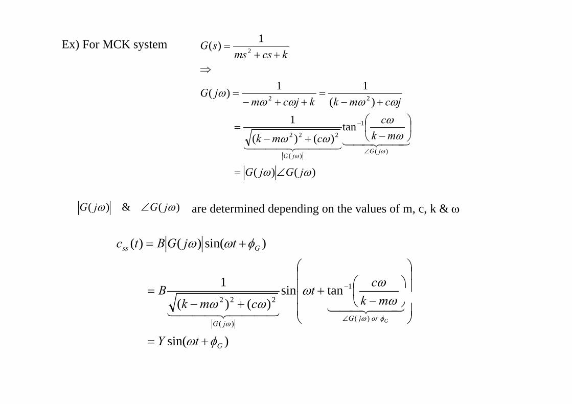
Ex) For MCK system 1)( 2 kcsmssG
)(11)( 22
jcmkkjcm
jG
tan)()(
1
)(
1
)(
222
mkc
cmkjG
jG
)()()(
jGjGjG
are determined depending on the values of m, c, k & )(&)( jGjG
)sin()()( Gss tjGBtc
tansin1
)()()(
1
Gss
ctB
j
)sin(
tansin)()(
)()(
222
orjGjG
tY
mkt
cmkB
G
)sin( GtY

Frequency response of a linear system
js
sGjG
)()(
Linear system )sin()( GtjGB )()()( jGjGjG
tB sin
- Output has same frequency with input frequency!
- Output depends on the magnitude & phase of the system)( jGG )( jG
Comments
Output depends on the magnitude & phase of the system)( jGG )( jG
)()()(
jRjCjG Output sinusoid’s magnitude
Input sinusoid’s magnitude=- Amplitude ratio:
)(C
Input과 output의magnitude와 phase를알면 즉 G( )를
)()()()()(
jRjC
jRjCjGG - Phase shift
알면 system 즉 G(s)를재구성가능
G : phase shift 0G0G
: phase lead
: phase lag
Output to input sinusoidCss(t)=B )sin()( GtjGB )( jGB
Input sinusoidr(t)=
2
T tB sin

B. Plotting Frequency Response
jssGjG
)()(
- Frequency response of a system G(s)
- Frequency response characteristics (주파수응답특성) : Sinusoidal input의 frequency 의값에따라 system output의
magnitude와 phase angle이변화하는 system의성질magnitude와 phase angle이변화하는 system의성질
- Graphical representation of frequency response characteristics
1) Bode plot (logarithmic plot):- plotting magnitude (dB) and phase ( ) of a system vs. frequency (log ) separately
)(
2) Polar plot (Nyquist plot):- plotting magnitude and phase in complex plane
Note. dB (decibel) = 20 log )( jG

Ex10.1) Find analytical expression for the frequency response for a system G(s) = 1/(s+2). And plot them in Bode and polar plot
jssGjG
)()(Frequency response for a system G(s)
221)(
jjjG
4442)( 222
jj
jG
Real part imaginary part
GGMjG )(
magnitude 144
2)(2
2
2
2
jGM G
Method I)
Analytical expression for the frequency response of a system
2tan2
4tan)( 12
1
jGG
g444
)(222
jG
phase
24
22
Method II) Magnitude: 분모/분자의크기를따로계산후나누기
p
41)(2
jGM G
kk
jj
M
M
Phase: (분자항들의 phase의합) –(분모항들의 phase의합)
2tan
2tan
10tan)( 111 jGG
kk
jj pz )()(
Phase: (분자항들의 phase의합) –(분모항들의 phase의합)

1) Bode plot
20log0.35=-9.12dB
4
1log20log202
GM
logog
2tan 1 G
-45o
2) polar plot
2 rad/s
) p p
2tan1
)()(
1
GGM -45o
242
12
if
4535.02
tan4
1 1
2

Interpretation of the Bode plotInterpretation of the Bode plot
FilterL filt- Low pass filter
- High pass filter- Band pass filter
M-C-K system

Asymptotic Approximations: Bode Plots
Simplifying the sketching Bode plots by straight-line approximations
)())(()( 21 kzszszsKsG
)())(()(
21 nm pspspss
sG
Magnitude frequency response
jsn
mk
pspspsszszszsK
jG
)()()()()()(
)(21
21
Multiplication/division
converting into dB by taking the logarithm
zszsKjG )(log20)(log20log20)(log20 21 Al b i / b i
js
m pss
)(log20log20 1
21 Algebraic sum/subtraction
Phase response
Much easier for graphics!
j
m pss
zszsKjG
)(
)()()(
1
21
Advantage of the Bode plot js
p
)( 1(logarithmic plot)

Basic factors of Bode plots
1. Gain Knj )(
nTj )1(
1. Gain K
2. Integral and derivative factors
3. First-order factors
n
nn jj2//21 4. Quadratic factors
* Once logarithmic plots of these basic factors are known, Bode plots of complicated function can be Once logarithmic plots of these basic factors are known, Bode plots of complicated function can be constructed easily by adding individual curves of each factors
2221 )())(()( kzszszsKsG
2221 2)())((
)(nnn
m sspspspss
* Note. Always make transfer function in normalized form when to draw Bode plots s
11121 k ssszzzK
1)(
asaas
12111
111)(
2
21
212
21
m
knn
ssps
ps
pss
zzzpppK
sG
21 nnnppp

a. Bode plots for Gain K
KjGdB log20)(log20 0 K
KsG )(: constant
: No angular contributiong
dB
Klog20
Note
0.1 1 100o
log
Note. If K >1, dB>0
K<1, dB<0
Effect of varying gain K: raises or lowers ther log-magnitude curve of the transfer function by , but no effect on the phase curve!Klog20

b. Bodes Plots for Integral and Derivative factors nssG )(
njjG )( log20)(log20 njGdB
jjjjti
n
jjjn
timesn
tan 1
ni
90
01
Bode plots using straight line asymptotes
slopedB
n = +2+40 dB/decade
40 +180o n = +2
slope
0 1 1 10 log
n = +1+20 dB/decade20 +90o n = +1
log0.1 1 10 g
n = -2
n = -1-20 dB/decade
-20-40
- 90o
- 180o n = -2
n = -1g
n 2-40 dB/decade
* Decade: 10 times the initial frequency


C. Bodes Plots for first-order factors
js let
1loglog20)(log20
2
anjGdB
nassG )()( From constant a
nn
ajaajjG
1)()(
gg)(ga
j
n
i
n
i
n
i
n
aaaaja
1
1
1
1
1
1 tantan0tan1
Normalize it first!
If
Straight line asymptotes
aei ..1 andB log20 0tan 1
a
Normalize it first!
a
a
aora
1 na
45tan 1 If 2loglog20 andB
If aora
1 log20log20 na
adB
n
a
90tan 1
B k ( )From constant a
+180o
+90o
n = +1
n = +2Rough estimatedB
n = +1
n = +2
+20 dB/decade
+40 dB/decade
20
40
Break (corner)frequency
an log20
an log20 +90
- 90o
0.01a a 100a logn = -1
0.1a 10a+45o
0.01a a 100a log
n = -1-20 dB/decade
+20 dB/decade20
-2040
0.1a 10a0
an log20
an log20
l20an log20
Actual vs. asymptotes?- 180o n = -2n = -2
-20 dB/decade
-40 dB/decade
-40
Decade:10 times the initial frequency
an log20

Comparison between andn
assG
1)(2
nassG )()(1
n
n
nnn
asasGassG
1)()()(
assG
1)(2
Bode plot of G2(s) l it d l t f G ( ) b l20
Magnitude shift by an log20
lower magnitude plot of G1(s) by Same phase plot
an log20
+180o
n = +2
Rough estimatean log20
dB
n = +1
n = +2+40 dB/decade40
Break (corner)frequency
For G1(s)
+90o
0.01a a 100a log
n = +1
0.1a 10a+45o
0.01a a 100a log
n = 1
n = +1+20 dB/decade20
-200.1a 10a0
an log20
an log20an log20
- 90o
- 180o n = -2
n = -1
n = -2
n = -1-20 dB/decade
-40 dB/decade
20-40an log20
an log20
For G2(s)0
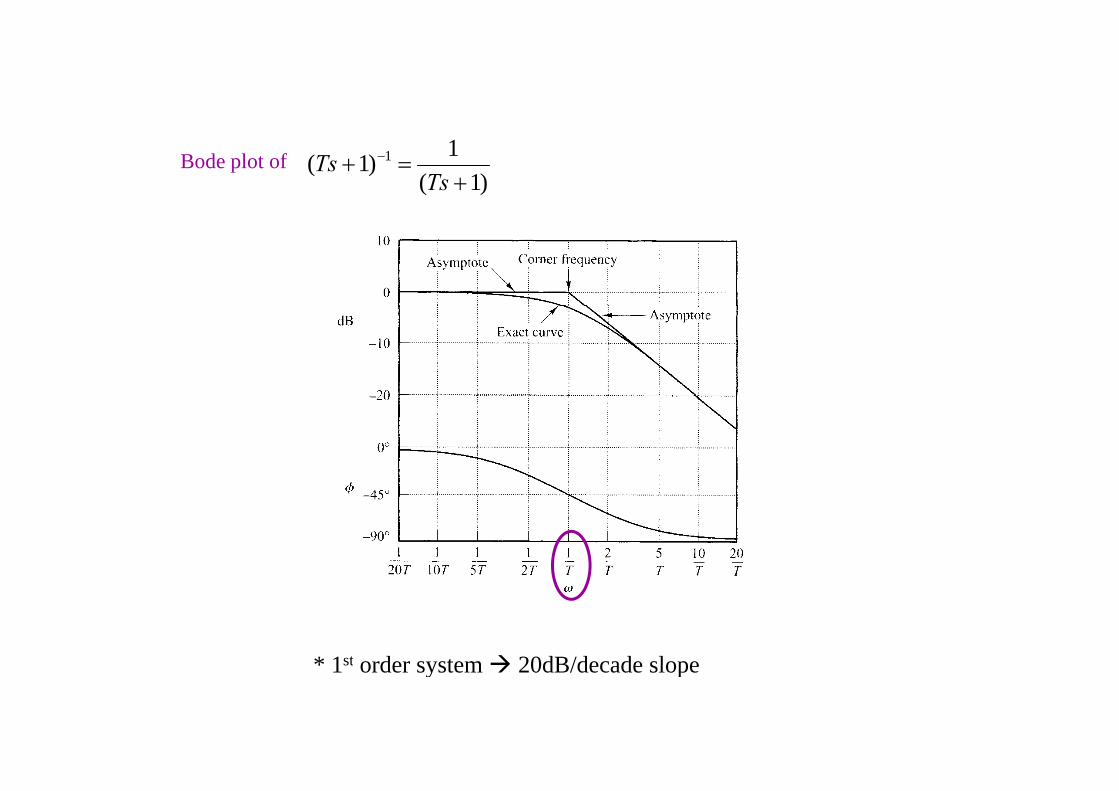
)1(1)1( 1
TsTsBode plot of
* 1st order system 20dB/decade slope* 1st order system 20dB/decade slope

Ex) draw Bode plots for the following system where )2)(1(
)3()(
ssssKsG
Bode plot using open-loop TF )()()()()()( 212121 jGjGjGjGjGjG p g p p sum of each first-order terms )()()()( 2121 jGjGjGjG
1
323 sK
N li f it l f i i 0 dB
1
2)1(
32)(sss
sGNormalize for unity low-frequency gain, i.e. 0 dB

D. Bodes Plots for 2nd-oerder factorsn
nn
nn
nn
sssssG
12)2()( 2
2222
n
nn
jjjGn
12)(
22
Normalized form
22
2
22 21loglog20)(log20
nn
nnjGdB
21
2
22
2
22
1
2tan2121 n
n
n
n
n
n
njjn
n
n
n
Straight line asymptotes
1n
nn nn
If
Straight line asymptotes
nn
ei
..1 010tan 1
nn nndB log401loglog20 2
If 1800t 1
900
tan 1 nn
If
ei 1 l40l20
22
2dB
nn
ei
..1 2loglog20 2 n
ndB
1800tan 1 nn nn
ei
..1
log40log20 22 nndB
n
n
Function of damping ration

+360o
+1
n = +2Rough estimatedB
n = +2+80 dB/decade
80Break frequency
n = +1+40 dB/decade
nn log40
+180o
- 180o0.01 100
n = -1
n = +1
0.1 10+90o
0.01 100 log
40
400.1 100
40 dB/decade nn log40
nn log40
n log40n n n n n n n n n
n log
- 360on = -2
n 1
n = -2-80 dB/decade
-40-80 n = -1
-40 dB/decadenn log40nn log40
* 2nd order system 40dB/decade slope
1)( 222
2
nsG
0 for standard form
12)2(
)( 222
nn
n ssss n
dB80 +360o
Function of damping*magnitude shift by nn log40
0.01 100 log
40
400.1 100
n n n n n
+180o
0.01 1000.1 10n n n nn log
-40-80 n = -1
-40 dB/decade
- 180o
- 360o

Actual response vs. asymptotic approximation of)2(
1)( 22n
sssG
n
- Greater disparity depending on
- Correction factor for actual shape 2log20 pg
R f ei 1
707.0There’s no resonant peak for
Resonant frequency nn
ei
..1
To be exact 222
2 21
1)(
jG
22 21
nn
n
Should be minimum @ resonant frequency r
0 r
dd
nnr 221resonant frequency

1st d 2nd d t1st order vs. 2nd order system
dB80 +180o
0.01 100 log
40
80
0.1 100n n n n n
+180o
+90o
0 01 1000 1 10 log-40-80
2차 system
n n n n n
- 90o
- 180o
0.01 1000.1 10n n n nn log
1차 system 1차 system
2차 system
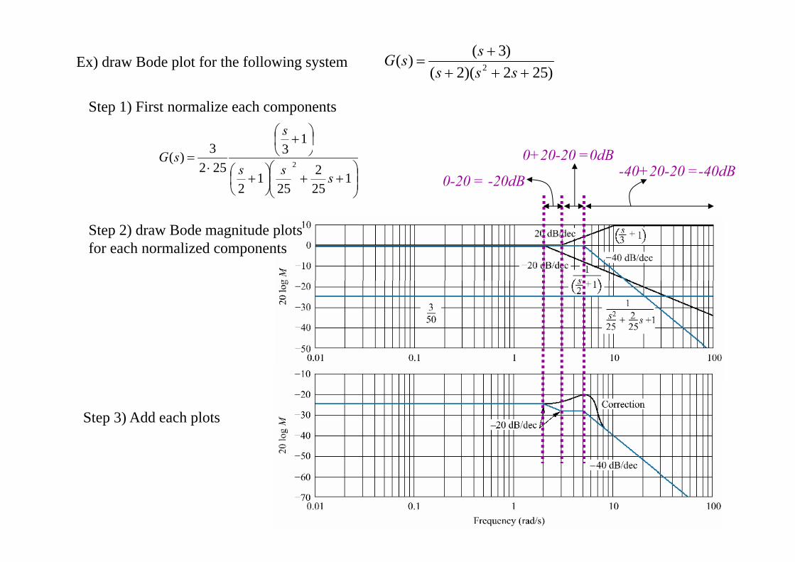
Ex) draw Bode plot for the following system)252)(2(
)3()( 2
sss
ssG
Step 1) First normalize each components
1
33)(
s
G 0+20 20 =0dB
1252
251
2
3252
)(2
ssssG
0-20 = -20dB
0+20-20 =0dB-40+20-20 =-40dB
Step 2) draw Bode magnitude plots for each normalized components
Step 3) Add each plots

Step 4) draw each Bode phase plots for each normalized components
Step 5) Add each plots
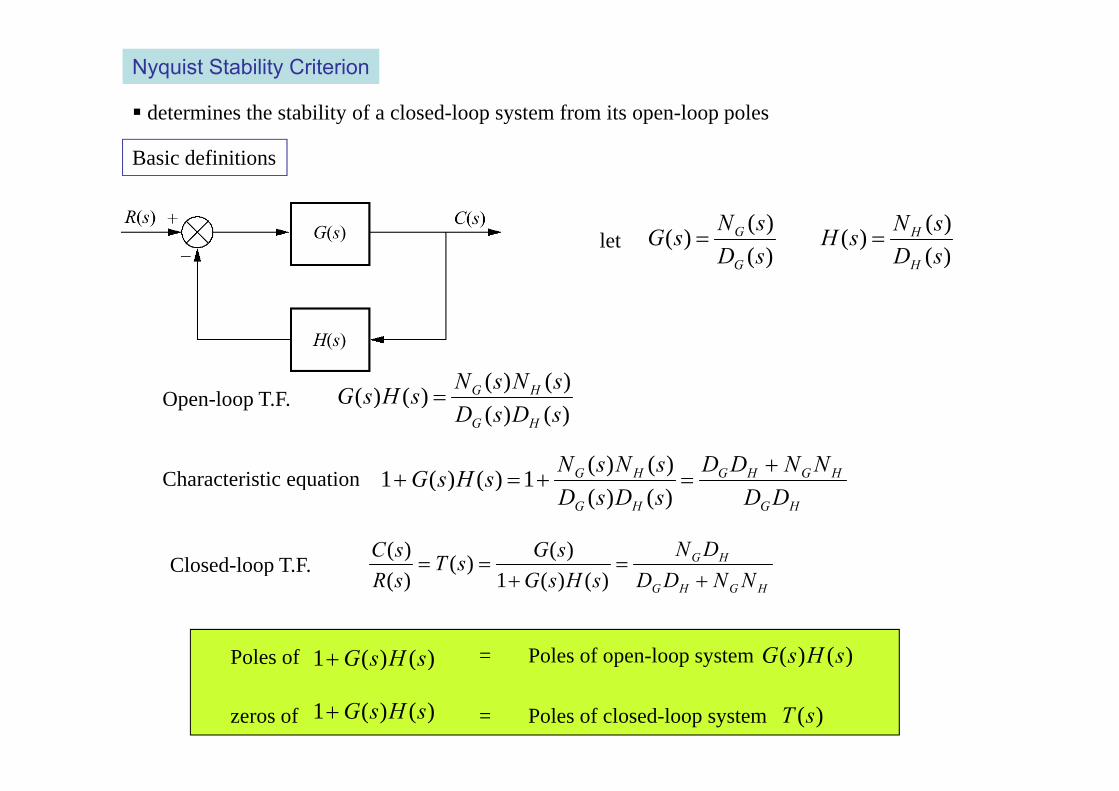
Nyquist Stability Criterion
determines the stability of a closed-loop system from its open-loop poles
)(N )(N
Basic definitions
)()()(
sDsNsG
G
G)()()(
sDsNsH
H
Hlet
)()()()( sNsNsHsG HGO l T F)()(
)()(sDsD
sHsGHG
Open-loop T.F.
HGHGHG NNDDsNsNsHsG
)()(1)()(1Characteristic equation
Closed-loop T.F.
HGHG DDsDsDsHsG
)()(1)()(1Characteristic equation
HG
NNDDDN
HGsGsT
RsC
)()(1
)()()()(
pHGHG NNDDsHsGsR )()(1)(
Poles of )()(1 sHsG = Poles of open-loop system )()( sHsG)()(1 sHsG p p y )()(
zeros of )()(1 sHsG = Poles of closed-loop system )(sT

Mapping
F(s): any complex functionA. Mapping of a complex numberAny complex number on s-plane Another complex number on F-planeF(s) js
12)( 2 sssF
Plug in
jωS-plane F-plane
12)( sssF
34 js
12 j
3016 js Im F(s)
σ
1)(
ssF
12 js
12 js
Mapping Re F(s)
1)(
ssF j
34 js in s-plane are mapped into
3016 js in F-plane through the function 12)( 2 sssF
12 js 12 js 1)(
ssF12 js 12 js
1)(
ssF
B. Mapping of a contour
Contour (closed-curve): collection of points
pp g
Maping contour A to contour B through function F(s)

Contour mappinga beSkip pp g
F(s) ?cd
Pole s
sF 1)( zero ssF )(
901901
101
j
11
90110 j
45211 j
@a
@b 452
452
452
111
1
j
452
111
1
j
45211 j
45211 j
@b
@c 211 j
크기: 반비례Phase: 반대 (+/-)(시계반시계)
크기: 비례Phase: 비례 (+/-)(시계시계)(시계반시계) (시계시계)

Properties of contour mapping
Assuming clockwise direction of contour A
1. If one zero is inside of contour A complete CW encirclement(360o) about the origin of F(s) planeone pole CCW encirclement (-360o)
g
2. If the pole or zero of F(s) is outside of contour A, Contour B does NOT encircles the origin of the F-plane
3. If both the zero and the pole are in the contour A, then?

For example
V t t ti f i))()((
))((1)(543
21
pspspszszsGHsF
For example
Vector representation of mapping
As we move around contour A in a clockwise direction,
each vector inside contour A Undergoes a complete rotation or 360o angle change
Clockwise rotationCounter-clockwise rotation
each vectoroutside contour A oscillate and return to its position or a net 0o angular change
543
21)(VVV
VVjFR 00360360360
)( 54321
VVVVVsF
Counter clockwise rotation
360oZ - 360oP 360 ( )
360 One clockwise rotation
Z : Number of zeros of 1+G(s)H(s) inside contour A
= 360o (Z-P)
N
ZP
: Number of clockwise rotations of contour B about the origin
: Number of zeros of 1+G(s)H(s) inside contour A: Number of poles of 1+G(s)H(s) inside contour A
For this case Z = 2, P=1 N=1
PZN If N is related to counterclockwise rotation, then obviously N = P - Z

Z : Number of zeros of 1+G(s)H(s) inside contour A = # of Poles of closed loop system )(sT
Not known
Z
P
: Number of zeros of 1+G(s)H(s) inside contour A = # of Poles of closed-loop system
: # of poles of 1+G(s)H(s) inside contour A = # of poles of open-loop system )()( sHsG
)(sT
known
PNZ # of closed-loop poles inside the contour =# of clockwise rotations of mapping about the origin +# of open-loop poles of G(s)H(s) inside the contour
As system stability is determined by closed-loop poles in RHP, let’s consider the entire RHP has the contour
0Zi.e.at least one closed-loop pole exist in RHP unstable
0Z No closed-loop pole exists in RHP stable0Z No closed loop pole exists in RHP stable
P Easily found by examination of open-loop TF G(s)H(s)
As long as N is found, then system stability can be determined Z = N + Pg , y y
# of closed-loop poles in RHP =
Nyquist Stability Criterion PNZ p p
# of clockwise rotations of mapping about the origin + # of open-loop poles of G(s)H(s) in RHP
1+G(s)H(s)

Mapping through G(s)H(s) instead of 1+G(s)H(s) Translate the contour B made by 1+G(s)H(s) one unit to the lefty ( ) ( ) f consider the rotations about -1+j0 instead of about the origin
jωG(s)H(s) l 1+G(s)H(s)
jωplane 1+G(s)H(s)
plane1+G(s)H(s)
plane
G(s)H(s) plane
jω
σ σ-1-1
σ0
p
Contour B made byG(s)H(s)(-1, 0) of 1+G(s)H(s) plane
= origin of G(s)H(s) plane
Contour B made by1+G(s)H(s)
# f l d l l i RHP
Nyquist Stability Criterion PNZ # of closed-loop poles in RHP =
# of clockwise rotations of mapping about (-1+j0) + # of open-loop poles of G(s)H(s) in RHP
G( )H( )G(s)H(s)

Ex) N = 0P = 0Z=N+P= 0
Stable!
N = 2P = 0P = 0
Z=N+P= 2
Unstable!Unstable!

Sketching the Nyquist Diagram
Nyquist diagramNyquist diagram obtained by substituting points along the contour (i.e. entire RHP) into the function G(s)H(s)
1)( sHEx) 500)( sG 1)(sHEx)
contour (i.e. entire RHP)
)10)(3)(1()(
ssssG
( )
GH lIm G(s)H(s)
l
)10)(3)(1(500)(
ssssG
MappingThrough
GH-plane
Re G(s)H(s)
s-plane
Nyquist Diagram?
Through G(s)H(s)
i di ? S b i i h i i G( ) ( )
Nyquist diagram? Substitute every points on the contour into s in G(s)H(s)
: positive imaginary axis : infinite semicircle
Let
: negative imaginary axis
For convenience, let’s draw Nyquist diagram for separately and connect them later

Points on positive axis where ( i t b t A t C)
j js
A. Nyquist diagram for part (positive imaginary axis )
~0(points between A to C)
2322
32
32 )43()3014()43()3014(500
)43()3014(500
)10)(3)(1(500)()(
j
jsssjHjG
)43()3014()43()3014()10)(3)(1(
jsss js
500)()( jHjG
43tan0tan)()( 2
311 jHjG
magnitude phase
2322 )43()3014()()(
jj
3014
a500
a)()( 2 jjG
0 0500)( jG point A’When is small 0 030
)( jG
90500500500500)( 333 jjG
point AWhen is small, (= @ point A = @ low frequency)
When is large, 900
90)()10)(3)(1(
)( 333
jsss
jGs
point C’
g(= @ point C = @ high frequency)
When is middle range frequency(around point B)
(around point B)
1430
90)( jG Crosses the negative Im-axis0)(Re jG
43 874.0)( jG 180)( jGCrosses the negative Re-axis0)(Im jG

0 030500)( jG point A’
90090500)( 3
jG point C’
1430
90)( jG Crosses the negative Im-axis
8740)( jG 180)( jG43 874.0)( jG 180)( jGCrosses the negative Re-axis
43
1430
43

B. Nyquist diagram for part (points between C to D, i.e. around the infinite semicircle)
infinite semicircle jes
30)(
500)10)(3)(1(
500)( 3
jes esss
jGj
At point C , 90 2700)( C
jG point C’
At point D , 90
)(Cs
j
2700)( Ds
jG point D’
1
cossintansincossincos 122je jNote
Note.-It is OK to assume infinite semicircle maps into the origin- No need to calculation for - only when # of poles > # of zeros- only when # of poles > # of zeros
Mapping of the negative imaginary axis
C. Nyquist diagram for part (points on negative imaginary axis)
Mapping of the negative imaginary axis mirror image of the mapping of the positive imaginary axis
-Finished-

Note.-It is OK to assume infinite semicircle maps into the origin- No need to calculation for
=OK to assume both are same!

Special case: Open-loop poles exist on the axis j
Detour around (to the left or right) the poles on the axisjDetour around (to the left or right) the poles on the axis
Detour must be infinitesimally small to to include some closed-loop poles jes
j
Detour path infinitesimal semicircleN tNote.
ajajes j
bj bjes j
Ex) Sketch the Nyquist diagram of the following unity-feedback system where 2
)2()(s
ssG
V1
V2
Bypassed contour Nyquist diagram

I) Rough sketch
)2(s
2
)2()(
jjG
2
)2()(s
ssG
2
0 2
point A’0
9002)( 2
jjjG point B’
18002)( 2
jjG
infinite semicircle maps into origin because # poles > # zeros)( jG
jes infinitesimal semicircle
2)(
2)(2)2()( 222
jj
j
es eee
ssjG
j
At point F 0
0)( 0 jjG point F’
At point A, 90
At point E 90
180)( 90
jesjG
point A’
point E’180)( jG
At point F, 0 )( 0 jesj
p
At point E , 90 point E 180)( 90 jesjG
Negative Im-axis mirror image of the mapping of D’ to E’

II) More detail
At middle frequencies range in between A & BAt middle frequencies range in between A & B
Both real and imaginary part of are negative should be in 3rd quadrant)( jG
jjjes infinite semicircle
0)()(
2)2()( 222 j
j
j
j
es ee
ee
ssjG
j
At point B, 90 900)( 0 jjG point B’
At point B, 900)( 0 jesjG p
At point C, 0 00)( 0
jesjG point C’
At point D, 90 900)( 0
jesjG point D’

Stability via the Nyquist Diagram
For closed-loop system that has a variable gain in the loop, for what range of gain is the system stable?
PNZ
For closed loop system that has a variable gain in the loop, for what range of gain is the system stable?1. Root locus2. Routh-Hurwitz3. Nyquist criterion
For various values of gain K, how to draw the Nyquist diagram?Set the loop gain K= 1Draw the Nyquist diagramMultiply the gain anywhere along the Nyquist diagram (since gain is simply a multiplying factor)
- As K increases, Nyquist diagram expands- As K decreases, Nyquist diagram shrinks
OrOr Nyquist diagram remains stationary and consider the critical point (1/K, no more -1+j0) moves
along the real axis

Shrinked Nyquist diagram with small gain KN = 0, P =2, Z=2 Unstable!
Expanded Nyquist diagram with large gain KN = -2, P =2, Z=0N 2, P 2, Z 0Stable!
-1
contourNyquist diagram
contour
Gain K should be large to make N=-2 since P =2 (Stable!)If K i ll h i i l i 1/KIf K is small, then critical point 1/K would be located outside the Nyquist diagram N = 0 Unstable!
1/K < 1.33 K > 1/1.33

Ex) find the range of gain K to make the unity feedback system stable where)5)(3(
)(
sss
KsGSet the loop gain K= 1 and Draw the Nyquist diagramMultiply the gain anywhere along the Nyquist diagramMultiply the gain anywhere along the Nyquist diagram
2224
32
)15(64)15(8
)5)(3()()(
j
jjjKjHjG
Point A where the Nyquist diagram intersects the negative real axis15 Set the imaginary part to be zero
Value of real part? -0.083
Point A where the Nyquist diagram intersects the negative real axis
A
Since P=0, N should be zero to be stable Point A should stay left to the -1+j0 Nyquist diagram can be expanded before point A meets -1+j0 gain K( 1) can multiplied (or increased) 1/0 0083 120 5 times before the system becomes unstable
K<120.5For stability
gain K(=1) can multiplied (or increased) 1/0.0083 =120.5 times before the system becomes unstable
At K=120.5, point A meets critical point -1+j0, system becomes marginally stable and system oscillates at the frequency of rad/sec15

Stability via Mapping Only the Positive axisj
open-loop magnitude at the frequency where the 180
)()(
jHjG
phase angle is 180o(or -180o)
)()( jHjGopen-loop magnitude at the frequency where the phase angle -135o
135)()(
jHjG
Encirclement of critical point
Can be determined from the open-loop magnitude at the frequency where the phase angle is
j
p p g q y p g180o(or -180o)
Can be determined from the mapping of the positive -axis alone, i.e. A’B’(because infinite semicircle maps into origin when # poles > # zeros)
Positive -axis (AB) A’B’j
(because infinite semicircle maps into origin when # poles > # zeros)
D h N i di di h i i f hDraw the Nyquist diagram corresponding to the -axis portion of the contourj

Ex 10-7) determine the stability range of K for the unity feedback system )2)(22()( 2
sssKsG
22222
22
2 )6()1(16)6()1(4
)2)(22()()(
jsss
KjHjGjs
First, draw the portion of the contour only along the positive imaginary axis
180201
201
j
Intersection with the negative real axis imaginary part = 0 6
Put it back to equation real part =
Portion of contour( axis only)
magnitude of open-loop
j
Nyquist diagram drawn from mapping of -axis only with the assumption K=1j
Nyquist diagram can be expanded 20 times before it becomes unstable (1/20 1) K can be increased 20 times more than the current value (K=1) before it becomes unstable
K<20 : stableK<20 : stableK=20 : marginally stable (oscillation frequency ) K>20 : unstable
6

Gain Margin and Phase Margin via the Nyquist Diagram
Gain margin GM or Kg
Indicates immunity to the parameter variation
g- Amount of open-loop gain variation allowed at 180o phase angle before the closed-loop system becomes unstable- reciprocal of the real-axis crossing point (open-loop magnitude) expressed in decibels (dB)
Phase margin M or - Amount of additional open-loop phase shift (lag) allowed at unity gain before the closed-loop system becomes unstable
Assume N should be 0 for the stability
Nyquist diagram can be expanded a times before it becomes unstable (1/a 1) K can be increased a times more than the K can be increased a times more than the current value (K=1) before it becomes unstable Gain margin = a or 20log a
Represents system’s proximity to instabilityAt unity gain, the system becomes unstable if h hift f dif a phase shift of degrees occur phase margin =

)()(1
jHjGPositive gain
margin)()(
1 jHjG
Negative gain
marging g
Positive phase
margin
-1Negative
phase margin
-1
margin g)()( jHjG
Stable UnstableEx 10-8) Find the gain and phase margin for the system of Example 10-7 if K=6Ex 10 8) Find the gain and phase margin for the system of Example 10 7 if K 6
Simply multiply 6 to all the results of Ex (10-7) in which K= 1
22222
22
2 )6()1(16)6()1(46
)2)(22(6)()(
j
sssjHjG
)6()1(16)2)(22( sss js
1803.06201
real axis crossing Gain margin = 20 log (1/0.3) = 10.45dBGain margin
Phase margin 1
)6()1(16)6()1(46)()( 22222
22
jjHjGSolve for for which the magnitude =1
sec/253.1 rad
Phase margin
sec/253.1 rad 3.112
)6()1(16)6()1(46)()(
253.122222
22
253.1
jjHjG Phase margin = 180-112.3
= 67.7o

Gain Margin and Phase Margin via the Bode Plot
Bode plot - Easily drawn without long calculations required for the Nyquist diagram- but gives the same information (stability, gain and phase margin, range of gains for stability)obtained by Nyquist diagram
- Viable alternative to Nyquist plots- Viable alternative to Nyquist plots
GM and PM via Bode plot

Ex 10-9) Find the range of gain K for the stability of the unity feedback system where
Stability via Bode plot
Ex 10 9) Find the range of gain K for the stability of the unity feedback system where
)5)(4)(2()(
sssKsG
1
51
41
2
40/)(sss
KsG
Requirement of stability (from Nyquist stability concept)- N=0 (because P=0)- magnitude of open-loop <1 at 180o (i.e. 20 log |G| < 0dB)
20 log K/40 20 log K/40-20
20 log K/40-40 G|
GM20 log K/40 40 20 log K/40-60
20 log K/40-80 20 log K/40-100 20 log K/40 120
20 lo
g |
at 180o, sec/7rad
20 log |G| = 20 log K/40 20 <020 log K/40-120 20 log |G| = 20 log K/40 -20 <0
For stability: 0<K<400
Note. Same results can be obtained by Nyquist diagram which requires long computation
PM
long computation

Ex 10-10) Find the GM and PM when K=200 for the same system in Ex 10-9
GM = 6.02dB
Gain margin: gainGain margin: gain required to raise the magnitude curve to 0 dB
PM = 15o
- For stable system, GM (dB) >0 & PM >0- for unstable system, GM (dB) <0 & PM <0
Remarks on GM and PM
- Optimal GM> 6dB- Optimal PM : 30o~60o
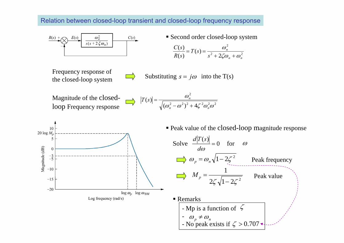
Relation between closed-loop transient and closed-loop frequency response
Second order closed-loop systemSecond order closed loop system
22
2
2)(
)()(
nn
n
ssT
sRsC
Frequency response of the closed-loop system js Substituting into the T(s)
2
222222
2
4)()(
nn
nsT
Magnitude of the closed-loop Frequency response
Peak value of the closed-loop magnitude response
0)(
dsTd Solve for
d
Peak frequency221 np
1M Peak value2212
pM Peak value
Remarks
- Mp is a function of-- No peak exists if
np
707.0

BW Bandwidth of the closed-loop frequency response
Frequency at which the magnitude response curve is 3dB down from its value at zero frequency-Frequency at which the magnitude response curve is 3dB down from its value at zero frequency - indicates how well the system will track an input sinusoid- indicator of system speed
- Calculation of BW3
4)(log20)(log20
222222
2
nn
nsT
244)21( 242 nBW
sn T/4 BW
244)21(4 242
BW T
- By substituting , is related to settling time Ts
sT
244)21( 242
- By substituting , is related to settling time Tp21/ pn T BW
244)21(1
242
2
p
BWT
nrT
- By using Fig.4.16(NISE), is related to settling time TrBW

Relation between closed-loop transient and Open-loop frequency response
Relationship between the phase margin and the damping ratioRelationship between the phase margin and the damping ratio
A unity feedback system with an pen-loop TF
- enable us to evaluate the %OS from the phase margin obtained from the open-loop frequency response
)(2nsG
A unity feedback system with an pen loop TF)2(
)(nss
sG
22
2
2)(
)()(
nn
n
ssT
sRsC
C.L.T.F.
First find the frequency for which to evaluate the PM 1)( jG
12
)(2
2
n
jjG 42
1 412 n2 nj
Phase angle of at this frequency
2
tan90)( 111
n
jG)( jGq y
2142
tan9042
1
)180()( jGPhase margin42
1
1
2412
tan90
)180()(
jGMPhase margin
42
1
412
2tan
PM is a function of
damping ratio!

1 2t
42
1
412tan
M
221 np707.0We know that there is no peak for from
Implies that PM larger than 65 52o is required to ensure there is no peak inImplies that PM larger than 65.52 is required to ensure there is no peak in the closed-loop frequency response

Steady-State Error Characteristics from Frequency Response
Static error coefficients from Bode magnitude plotStatic error coefficients from Bode magnitude plot
)()()(i
Ni
psszsKsG
consider an open-loop TF
zK
i
iNs p
zsKsG
)(lim0
- At low-frequency region
Type 0, N = 0 pi
i KpzKjG log20log20)(log20
decdB /0slopeip
Type 1, N = 1 log20log20log20log20)(log20
Ks
Kpz
sKjG
i
i decdB /20
i t t th f i t
1izKizK K
slope
Type 2, N = 2 decdB /40 log40log20log20log20)(log20 22
KsK
pz
sKjG
i
i
intersects the frequency axis at
1i
i
pj
i
i
pK
vK
slope
12
i
i
pz
jK
i
i
pzK
aKintersects the frequency axis at
S t t d t i d f th l t th l f i
= 20dB/dec-slope curve가 frequency axis와교차하는주파수vKpK = 저주파영역에서의 magnitude ( )pKlog20
System type determined from the slope at the low frequency region Type Slope
0 0
1 -20p 가 q y 와 차하 주파수v
= (-40dB/dec-slope curve가 frequency axis와교차하는주파수)2aK 2 -40


Ex) Find the system type and the appropriate static error constant for the Bode magnitude plot
Initial slope: 0 dB/dec type 0
20log K = 25 K = 17.7820log Kp 25 Kp 17.78
Initial slope: -20 dB/dec type I
Initial -20dB/dec curve crosses 0 dB at 0.55 rad/sec Kv = 0.55
0.55
Initial slope: -40 dB/dec type II
Initial slope curve crosses 0 dB at 3 rad/sec Ka = 32 = 9
3

Obtaining Transfer Functions Experimentally
Construction of the transfer functionConstruction of the transfer function- using step response data- using sinusoidal frequency response data
how? how?- forcing the system with sinusoidal input- measure the output steady-state sinusoid amplitude and phase angle- repeating these process at a number of frequencies yields data for a p g p q yfrequency response plot- obtain the frequency response plot (Bode magnitude and phase plot) using the following relation
)( jC Output sinusoid’s magnitude)()()(
jRjCjG Output sinusoid s magnitude
Input sinusoid’s magnitude=magnitude:
)()()()()( jRjC
jRjCjGG Phase shift
-Once bode transfer function of the system can be estimated from the break frequencies and slopes
)( jR= Output sinusoid’s phase - Input sinusoid’s phase
frequencies and slopes

Guideline:
1. Determine the system type by examining the initial slope. 2. Difference between (# of poles) and (# of zeros) determined by examining the phase
excursion3 See if portions of the Bode plot represents obvious first- or second-order pole or zero frequency3. See if portions of the Bode plot represents obvious first or second order pole or zero frequency
response plots 4. See if there is any telltale peaking or depressions in the magnitude response plot that indicate
an underdamped second-order pole or zero, respectively5. If any pole or zero responses can be identified, overlay appropriate 20 or 40 dB/decade
lines on the magnitude curve or 45o/decade lines on the phase curve and estimate the break frequencies. For second order poles or zeros, estimate the damping ratio
d t l f f th t d d B d l tand natural frequency from the standard Bode plots6. Form a TF of unity gain using the poles and zeros found. Obtain the frequency
response of this TF and subtract this response from the previous frequency response. (Now you have a frequency response of reduced complexity)(Now you have a frequency response of reduced complexity)

Ex) Find the transfer function of the subsystem whose Bode plots are shown below
peak in the magnitude curve extract underdamped polesApproximate
peak 6.5dB from standard
sradnp /5
24.02nd order Bode plotThus, unity gain 2nd order system TF
25)(2
G n
subtract the Bode plot of G1(s) from the original Bode plot
254.22)( 2221
sss
sGnn
n
overlay -20 dB/decade line on the magnitude plot and a -45o/decade line on the phase plot Break frequency at 90 rad/s Break frequency at 90 rad/s
9090)(2
s
sG
Subtract the Bode plot of G2(s)
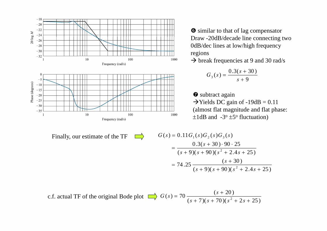
similar to that of lag compensator D 20dB/d d li ti tDraw -20dB/decade line connecting two 0dB/dec lines at low/high frequency regions break frequencies at 9 and 30 rad/sq
9)30(3.0)(3
sssG
subtract againYields DC gain of -19dB = 0.11 (almost flat magnitude and flat phase: 1dB d 3o 5o fl t ti )1dB and -3o 5o fluctuation)
)()()(11.0)( 321 sGsGsGsGFinally, our estimate of the TF
)2542)(90)(9()30(25.74
)254.2)(90)(9(2590)30(3.0
2
2
sssss
s
)254.2)(90)(9( 2 ssss
f l f h i i l d l)20(70)( sGc.f. actual TF of the original Bode plot
)252)(70)(7()(70)( 2
ssss
sG