Embed Size (px)
Citation preview

CFD prediction of thermal radiation of large, sooty,
hydrocarbon pool fires
(Vorhersage der thermischen Strahlung großer, rußender Kohlenwasserstoff-
Poolfeuer mit CFD Simulation)
by
Iris Vela
from
Šibenik, Croatia
Thesis submitted to the Department of Chemistry of
Universität Duisburg-Essen,
in partial fulfillment of
the requirements of the degree
Dr. rer. nat.
Advisor: Prof. Dr. Axel Schönbucher
Reviewer: Prof. Dr. Tammo Redeker
Date of disputation: April 30. 2009.
Essen, 2009.


Declaration
I declare that testimony that I have done the work alone. The sources and material used
here are completely described.
Essen, March 24. 2009.


Foreword
This thesis has been completed within the scope of a PhD program during my work as a
scientific assistant in the working group “CFD simulation of pool fires” in the Institute
for Technical Chemistry I at the University of Duisburg-Essen, Campus Essen.
For the topic of my scientific work, motivation and support through his knowledge and
scientific discussion I am thankful to Prof. Dr. rer. nat. Axel Schönbucher from the
Institute for Technical Chemistry I at the University of Duisburg-Essen, Campus Essen.
Great thanks to Prof. Dr. rer. nat. Tammo Redeker from the Technical University
Bergakademie Freiberg and IBExU Institute for Burning and Explosion Safety GmbH for
his high interest in my thesis and his cooperation as a reviewer. Also, many thanks to the
chair of this thesis, Prof. Dr. rer. nat. Reinhard Zellner.
Especially, I want express my thanks to my colleagues Dipl.-Ing. Markus Gawlowski,
Dr. Christian Kuhr and Dipl.-Phys. Peter Sudhoff from the Institute for Technical
Chemistry I at the University of Duisburg-Essen, Campus Essen, for the common work
and a support, also, to Dr. Wolfgang Laarz for help in many things during my work and
to Mrs. Lieselotte Schröder for her excellent administration, support and understanding in
many different situations. In addition, I want to thank other colleagues from the Institutes
for Technical Chemistry I and II at the University of Duisburg-Essen, Campus Essen for
a support and friendly working atmosphere.
Also, I want to thank for the cooperation with BAM Berlin, especially to Prof. Dr. K.-
D. Wehrstedt, the head of Division II.2 "Reactive Substances and Systems" in the Federal
Institute for Materials Research and Testing (BAM) for opportunity to participate in the
large-scale experiments on kerosene and peroxide pool fires.
In addition, thanks to Ms. K. E. Kelly, Prof. Dr. J. S. Lighty, Prof. Dr. A. Sarofim, Prof.
Dr. P. J. Smith, Dr. J. Spinti from the Institute for Clean and Secure Energy (ICSE),
University of Utah, Salt Lake City as well as to Dr. J. C. Hewson from Sandia National
Laboratory (SNL), Albuquerque and Dr. C. Shaddix from Sandia National Laboratory
(SNL), Livermore for cooperation and participation in Fire Workshops, and interest in
my work.


Content
Abstract
Nomenclature
1 Introduction………………………………………………………………………...1
2 Some characteristics and modeling of pool fires…………………………............3
2.1 Burning velocity and mass burning rate……………………………………...........6
2.2 Flame geometry…………………………………………………………..….…...11
2.2.1 Flame length…………………………………………………………………....11
2.2.2 Flame tilt…………………………………………………………………..…....16
2.2.3 Flame drag………………………………………………………………….......18
2.3 Flow velocities……………………………………………………………...........18
2.4 Flame temperature………………………………………………………….….....20
2.5 Organized structures……………………………………………………………...24
2.5.1 Reactive zone……………………………………………………………….…..24
2.5.2 Hot spots………………………………………………………………………..25
2.5.3 Soot parcels…………………………………………………………………….26
2.6 Thermal radiation models ………………………………………………………..28
2.6.1 Semi-empirical radiation models……………………………………………….28
2.6.1.1 Point source radiation model (PSM) ……………………………………...…29
2.6.1.2 Solid flame radiation models (SFM, MSFM) ……………………………….31
2.6.1.3 Two zone radiation models (TZM) ……………………………………….....34
2.6.2 Organized structures radiation models (OSRAMO II, OSRAMO III) ………...35
2.6.3 Radiation model according to Fay……………………………………………...40
2.6.4 Radiation model according to Ray……………………………………………..41
2.7 Irradiance………………………………………………………………………....41
2.8 Field models and integral models………………………………………………...44
2.9 CFD simulation…………………………………………………………………..45
2.10 Wind influence………………………………………………………………….48
3 Experiments…………………………………………………………………..…...51
3.1 Pools……………………………………………………………………………...51
3.2 Fuels…………………………………………………………………..………….52
3.3 IR thermographic camera system ……………………………………..…..….….52

Content
x
3.4 VIS camera system…………………………………………………..………......53
3.5 Radiometer measurements………………………………………..………….......53
3.6 Wind measurements………………………………………..………………….....55
4 Some important topics of CFD used in this work ……………………………....57
4.1 The conservation equations in fire modeling…………………………..….......57
4.1.1 Overall mass conservation………………………………………………….......59
4.1.2 Species mass conservation……………………………………………………..60
4.1.3 Momentum conservation……………………………………………………….61
4.1.4 Energy conservation………………………………………………………...….62
4.2 Sub-models in fire modeling…………………………………………………....63
4.2.1 Modeling of turbulence………………………………………………………...65
4.2.1.1 k-ε and k-ω models….………………………………………………….…….67
4.2.1.2 Large Eddy Simulation (LES) ……………………………………………….68
4.2.1.3 Scale Adaptive Simulation (SAS) …………………………………………...74
4.2.2 Combustion models…………………………………………………………….76
4.2.2.1 Source terms of species on the basis of chemical reactions………………….76
4.2.2.2 Eddy dissipation…………...…………………………………………………77
4.2.2.3 Flamelet model ……………………………………………………………....78
4.2.3 Radiation models……………………………………………………………….82
4.2.3.1 Photometric sizes and radiation balance equation …………………………...82
4.2.3.2 Discrete Ordinate …………………………………………………………….86
4.2.3.3 Monte Carlo ………………………………………………………………….87
4.2.4 Soot models…………………………………………………………………….88
4.2.4.1 Magnussen …………………………………………………………………...88
4.2.4.2 Lindstedt ……………………………………………………………………..89
4.2.4.3 Tesner ………………………………………………………………………..92
4.3 ANSYS CFX and FLUENT software………………………………………….94
4.3.1 Discretisation methods and solution algorithms………………………………..94
4.3.1.1 Finite volume method………………………………………………………...94
4.3.1.2 Geometry and mesh generation………………………………………………96
4.4 Procedure of CFD simulation…………………………………………………..99
4.4.1 Geometry and meshing ……………………………………………………….100
4.4.1.1 Geometry and meshing for the fire in calm condition ……………………...100

Content xi
4.4.1.2 Geometry and meshing for the fire under the wind influence ……………...101
4.4.2 Initial and boundary conditions and time steps……………………………….102
4.4.3 Determination and configuration of sub-models……………………………...105
4.4.3.1 Sub-models for turbulence……………………………………………….....105
4.4.3.2 Sub-models for combustion………………………………………………....107
4.4.3.3 Sub-models for thermal radiation………………...........................................107
4.4.3.4 Sub-models for soot………………................................................................109
4.4.4 Modeling of absorption coefficient of the flame……………….......................111
5 Results and discussions……………….................................................................113
5.1 Instantaneous and time averaged flame temperatures………………..................113
5.1.1 Thermograms……………….............................................................................113
5.1.2 Histograms……………….................................................................................116
5.1.3 Probability density function (pdf) ………………............................................117
5.1.4 Temperature fields……………….....................................................................119
5.1.5 Axial and radial profiles………………............................................................128
5.2 Instantaneous and time averaged Surface Emissive Power (SEP) ……………..133
5.2.1 Four-step discontinuity function of temperature dependent
absorption coefficient………………………………………………….……...133
5.2.2 Thermograms……………….............................................................................135
5.2.3 Histograms……………….................................................................................137
5.2.4 Probability density function (pdf) ………………............................................140
5.2.5 Determination of SEP by isosurface of flame temperature……………….......141
5.2.6 Integration of incident radiation G for determination of SEP………………...146
5.2.7 Determination of SEP by irradiance as a function of distance………………..147
5.3 Instantaneous and time averaged irradiance……………….................................148
5.3.1 Virtual radiometers………………................................................................... 148
5.3.2 Prediction of irradiance……………….............................................................149
5.4 Wind influence ……………………………………………………………........152
5.4.1 Flame height, flame tilt, flame drag…………………………………………..152
5.4.2 Wind influence on surface emissive power (SEP), irradiance (E),
temperature and flow velocity…………………………………………….…..162
5.5 Validation of CFD results…...……………………………………………..........171
6 Conclusions…………………………………………………………………..…..175
References……………….........................................................................................177

Content
xii
CV
Publications
Abstract
Computational Fluid Dynamics (CFD) simulations of large-scale JP-4 pool fires with
pool diameters of d = 2 m, 8 m, 16 m, 20 m and 25 m in a calm condition, as well as
with pool diameters of d = 2 m, 20 m and 25 m under cross-wind conditions with
wind velocities in a range of 0.7 m/s < uw < 16 m/s are performed. CFD prediction of
emission temperatures T, surface emissive power (SEP) and irradiances E(Δy/d) at
relative distances Δy/d in horizontal direction from the pool rim is carried out.
Also, for the theoretical understanding of large pool fires, the time dependent flame
temperatures are of great interest.
CFD predicted vertical temperature profiles CFDT (x/d) for different relative radial
distances y/d = 0, y/d = 0.05 and y/d = 0.1 show that the absolute maximum flame
temperatures CFDmax,T (d) are away (y/d = 0.05) from the flame axis and depend on d:
1300 K (d = 2 m), 1250 K (d = 8 m), 1230 K (d = 16 m), 1200 K (d = 25 m) which
agree well with the measured temperatures max,expT (d) . CFD predicted radial
temperature profiles CFDT (r) dependent on x/d are in agreement with measurements.
For pool fire with d = 25 m, at x/d = 0.125 bimodal profiles CFDT (r) are found, while
for x/d = 0.25 unimodal temperature profiles CFDT (r) exist.
The CFD simulation of the "derived" quantity SEP requires a definition of the flame
surface. The present work presents three different ways to predict SEPCFD. The first
way is the determination of isosurfaces of constant temperature which is defined as
the flame surface. The second way considers that the flame surface results from the
integration of many parallel two-dimensional distributions of incident radiation G(x,
y) along the z-axis perpendicular to the xy-plane. In the third way a virtual wide-angle
radiometer is defined at the pool rim and the irradiance E(Δy/d) as a function of Δy/d
is simulated. To simulate the SEP, more exactly, a temperature dependent effective
absorption coefficient effæ (T)ˆ of the dissipative structures (reaction zones, hot spots
and soot parcels) and air as a four-step discontinuity function is developed.
CFD predicted CFDSEP (d) values of JP-4 pool fires, obtained by the third way, are:
105 kW/m2 (d = 2 m), 65 kW/m2 (d = 8 m), 45 kW/m2 (d = 16 m) and 35 kW/m2 (d =

Abstract
xiv
25 m). The CFDSEP value for d = 2 m under predicts the expSEP by a factor of 0.8
whereas a good agreement is found between CFDSEP (d) and expSEP (d) for d = 8 m,
16 m and 25 m. Based on the first way the CFDSEP values agree well with the
measured expSEP values if the flame surface temperature of 1100 K is used for d = 2
m, 500 K for d = 8 m and 400 K for d = 16 m and 25 m.
Instantaneous h(T), h(SEP) and time averaged histograms h(T) , h(SEP) , lead to
probability density functions of the emission surface temperatures (flame
temperatures) pdf(T) and the surface emissive power pdf(SEP) , determined by the
second way. For example, from the predicted CFDpdf(T ) and CFDpdf(SEP ) for d = 16
m the temperature and SEP are in the intervals of 648 K < CFDT < 1100 K and 10
kW/m2 < CFDSEP < 80 kW/m2. The measured values are in the intervals 633 K <
expT < 1200 K and 9 kW/m2 < expSEP < 114 kW/m2. The CFD predicted functions
pdf(T), pdf(SEP) are consistent with the measured pdfs.
CFD predicted time averaged irradiances CFD
E (Δy/d, d) under predicts the
measured exp
E (Δy / d) at the pool rim Δy/d = 0 for d = 2 m by a factor of 0.8 and
over predicts exp
E (Δy / d) up to the factor of 1.6 at Δy/d = 0.5 whereas for d = 8 m,
16 m and 25 m the irradiances CFD
E (Δy/d) agree well with the measured
expE (Δy/d) . For example,
expE (Δy/d, d) as a function of d at Δy/d = 0.5 the
following values are found: 28 kW/m2 (d = 2 m), 18 kW/m2 (d = 8 m) and 5 kW/m2 (d
= 25 m).
The wind influence on large pool fire is a complex phenomenon. CFD simulation
shows that the wind influences the flame length, flame tilt, flame drag, the flame
temperatures T, the SEP and the irradiances E. With increasing wind velocity uw from
4.5 m/s to 10 m/s CFDSEP and CFD
E (Δy/d) at the pool rim increase downwind by a
factor of about 2 – 6 for d = 2 m and by a factor of about 2 – 7 for d = 20 m. In both
cases CFD
E (Δy/d) do not increase if uw > 10 m/s as it is found in experiments. In the

Abstract xv
upper section of the flames, depending on the flame tilt and drag, a decrease of flame
temperature of several hundreds K is found.
With increasing wind velocity uw 2.3 m/s the predicted flame tilt from the vertical
becomes significant. The CFD results show that two counter rotating vortices at the
leeward side of the fire are formed at the minimum uw = 1.4 m/s as observed in
experiments. The predicted flame tilt and drag for d = 20 m begins from 20° and 1.1
at uw = 1.4 m/s and ends with 80° and 2.5 at uw = 16 m/s which agree with the
experimental data. In a case of d = 2 m the flame tilt and drag reach values of 60° and
2.5 for uw = 4.5 m/s and 80° and 2.8 for uw = 16 m/s as in the experiments.
Flame temperatures T, surface emissive power SEP, irradiances E and the wind
influence on large pool fires were at the first time predicted with CFD simulations.
The CFD predictions are generally in good agreement with the measured values.
The CFD simulations allow (for future), the estimation of wind effects and also the
important influence of multiple fires on the hazard potential.
The present work has, also shown that the hazard potential of large pool fires with
CFD simulations of the thermal radiation can be estimated much better than before.

Abstract
xvi

Nomenclature
A area (m2)
AF flame area (m2)
ahs area fraction of hot spots
ax area of a pixel, matrix element, in the thermographic image (m2)
Ap pool area (m2)
asp area fraction of soot parcels
AT isosurface of constant flame temperature (m2)
cp specific heat capacity (kJ/(kg K))
d pool diameter (m)
dA infinitesimal area (m²)
dG infinitesimal incident radiation (kW/m2)
ds infinitesimal distance (m)
dV infinitesimal volume (m3)
E irradiance (kW/m²)
e extinction coefficient
Fr Froude number
Frf flame Froude number
G incident radiation (kW/m2)
g gravitational acceleration (m/s2)
gT(T) pdf of temperature
gSEP(SEP) pdf of surface emissive power
h specific enthalpy (kJ/kg)

Nomenclature
xviii
H length of the visible flame (m)
Hcl length of the clear burning zone (m)
H/d relative visible flame lenght
HP length of the fire plume (intermittency region of the flame (m))
Hpul length of the pulsation flame zone (m)
hrim height of the pool rim (m)
(–Δhc) specific height of combustion (kJ/kg)
Δhv specific height of vaporization (kJ/kg)
I radiation intensity (kW/(m2 sr))
IB blackbody radiation intensity at temperature T (kW/(m2 sr))
k absorption coefficient (1/m)
l length (m)
L radiation intensity (W/(m2 sr))
M molar mass (kg/mol)
mf mass of fuel (kg)
fm mass flow rate of the fuel (kg/s)
fm mass burning rate of the fuel (kg/(m2 s))
N particle number density in Lindstedt soot model (1/m3)
Ns number of species
NT number of total images in a thermographic sequence
n0 spontaneous radical formation in Magnussen soot
p pressure (bar)

Nomenclature xix
pa ambient pressure (bar)
Q total heat release rate (kW)
cQ heat of combustion (kW)
bQ heat back from the flame to the pool surface (kW)
q thermal radiation per area (kW/m2)
s direction
SEP surface emissive power (kW/m2)
SEPact actual surface emissive power (kW/m2)
SEPhs surface emissive power of hot spots (kW/m2)
SEPi,j local emissive power of a pixel element (kW/m2)
SEPLS surface emissive power of luminous spots (kW/m2)
SEPsp surface emissive power of soot parcels (kW/m2)
SEPSZ surface emissive power of soot zones (kW/m2)
t time (s)
Δt time interval (s)
T emission flame temperature (K)
Ta ambient temperature (K)
Ti,j temperature of the pixel element (K)
Tin inlet temperature (K)
Tmax centerline maximum emission temperature (K)
tb burning time (s)

Nomenclature
xx
u velocity (m/s)
v velocity (m/s)
V volume (m3)
va burning velocity of liquid fuel (m/s)
vf burning velocity of fuel (m/s)
X specific concentration (mol/kg)
x axial coordinate in vertical direction (m)
xi, yi amount of component i
Y mass fraction
y radial coordinate in horizontal direction (m)
Δy horizontal distance from the pool rim (m)
Δy/d relative horizontal distance from the pool rim
Greek symbols
α absorbance of the receiving area element
α convective heat transfer (W/(m2 K))
ß view angle ( °)
βF, βE view angles referring to a flame element, receiver element ( °)
æeffˆ effective absorption coefficient of the flame (1/m)
ε dissipation rate of turbulent kinetic energy (m2/s3)
Fε flame emissivity
φ view factor (–)
λ thermal conductivity coefficient (W/(m K))
ρ density (kg/m3)

Nomenclature xxi
a density of air (kg/m3)
f density of fuel (kg/m3)
s density of soot (kg/m3)
σ Stephan Boltzman constant (5.67 × 10⁻⁸ W/(m2 K4))
τ atmospheric transmittance (–)
Ω solid angle (sr)
Indices
a ambient
act actual
B black body
b boiling
b back
c combustion
eff effective
exp experiment
F flame
f fuel
g gas
hs hot spots
i, j the position of the pixel element in thermogram
LS luminous spots
m mass

Nomenclature
xxii
max maximum
P pool
P plume
p pressure
pul pulsation
rad radiation
rim pool rim
s soot
sp soot parcels
SZ soot zones
T temperature
v vaporization
w wind
Miscellaneous
(––) time averaged value
< > spatial averaged values
max(a,b) maximum of a and b
i, j the position of the pixel element in thermogram
OSRAMO organized structures radiation model
pdf probability density function
s direction of propagation

1 Introduction
Accidental fire in process plants are often pool or tank fires e.g. Buncefield in
December 2005 [1,2]. These fires show a potential risk for humans and neighboring
facilities due to their thermal radiation, and formation of combustion products such as
soot particles. Such fires are relatively little investigated experimentally [3-11] and
especially with CFD simulations [9,12-19]. A key parameter for the prediction of
thermal radiation of such fires is the Surface Emissive Power (SEP) [1,3-7,11,14-
16,20-29]. It is usually defined as the heat flux due to the thermal radiation at the
surface area of the flame. The SEP is dependent on the geometry, so for the prediction
of SEP it is necessary to define a flame surface AF [1,3-7,14-16,20-28]. In the past
semi empirical models are used to determine the time average SEP value averaged
over the whole flame surface FA as it is assumed in the point source model (PSM)
[5,7,25] and the solid flame model (SFM) [5,7,14-16,20-25]. The area FA is usually
assumed to be a cylinder or has a conical shape [5,7,14-16,20-25] or can be
determined by pdf of different organized structures in a fire as is done in OSRAMO
II, III [1,3,4,7,26-28]. The actual act
SEP , the hs
SEP and the spSEP of hot spots and
soot parcels can be obtained experimentally by evaluation of thermograms in
combination with VIS images by detecting luminous and non-luminous zones
[3,4,7,20,21,26-28]. The heat flux from the fire which can be received with
radiometers at a certain distance from the flame is defined as irradiance E(Δy/d)
[3,4,7,16,25-28]. With the (empirical) radiation model according to Fay [22] and Raj
[23,24] local profiles of thermal radiation can be considered. Ray [23,24] gives a
criteria for the setting thermal radiation hazard zones around large hydrocarbon fires.
He criticizes the current radiation models which do not consider the effect of the
combustion dynamics associated with large size pool burning. According to Ray [24]
the application of Computational Fluid Dynamics (CFD) to predict the dynamics and
radiation from a realistic, large pool fire is still in its infancy.
CFD simulations of large pool fires are done, also to reduce the number of large-
scale experiments. CFD simulation offers spatially and temporally resolution of
thermal radiation inside and outside the fire as a function of the fire dynamics.
University of Utah [16] and Sandia National Laboratory (SNL) [9,12,16] use CFD
code to predict the heat flux to the container inside and outside the fire, Jensen et. al.

1 Introduction
2
[29] validates different radiation models to predict heat flux profiles inside and
outside the flame. By CFD the irradiances E(Δy/d) depending on relative horizontal
distances Δy/d from the pool rim can be determined by virtual radiometers
[3,4,7,27,28]. Some CFD simulations are done on large hydrocarbon pool fires
(kerosene, JP-4) under the wind influence with different wind velocities [9,16,19].
Sinai et al. [19] investigate influence of the computational geometry on the predicted
flame tilt and drag and a temperature as a consequence, SNL investigate and their
influence of the flame tilt and drag on the temperature and thermal radiation from the
fire to the surrounding, especially on the heat flux to the container involved in a fire
[9,16,18].
In this work the CFD simulations of sooty, large, hydrocarbon pool fires e.g. JP-4
with d = 2 m, 8 m, 16 m, 20 m and 25 m are done to predict the emission temperatures
(T), the surface emissive power (SEP) and the irradiances (E(Δy/d)). The large JP-4
pool fires with d = 2 m, 20 m and 25 m are also investigated by CFD under the
influence of the cross wind with various wind velocities (0.7 m/s ≤ uw ≤ 16 m/s) to
predict the influence of flame tilt and drag on the CFDSEP and CFD
E (Δy/d).

2 Some characteristics and modeling of pool fires
Pool fire is defined in the literature [25] as the combustion of material evaporating
from a layer of liquid (fuel) at the base of the fire. It is generally turbulent, non-
premixed, diffusion flame, which liquid fuel is spread out horizontally [7]. Pool fire is
a kind of frequent accidental fires, which can occur in process industries by
spontaneous release of liquid fuels during their storage, processing or transport. A fire
in a liquid storage tank and a trench fire are also forms of a pool fire. A pool fire may
also occur on the surface of flammable liquid spilled onto water. For the fire
occurrence the relevant facts are the quantity of fuel in the fuel/air mixture,
geometrical properties of the fire environment, temperature conditions and a heat
transfer.
In the following chapter some physical and chemical properties of the pool fires are
discussed.
There exists a different kinds of open fires produced by ignition of accidentally
released flammable materials (liquids, droplets, gases or aerosols): pool fire, spill,
tank fire, boilover fire, flare flame, jet flame, fire-gas/clouds, UVCE, BLEVE,
fireball. The release scenarios, which can occur in chemical plants these types of fires
have a significant hazard potential, particularly due to the heat radiation and
convection, and the formation of combustion products (e.g. soot particles). The types
of fires can be characterized as follows [7]:
a) Pool, spill and tank fire:
Pool fire is defined as the combustion of material, usually a liquid or a solid which
can occur in a relatively thin layer on the surface of water or it can fill a pool.
In the case of fire spillage or leakage the flammable liquid spreads and form a spill on
some surface (e.g. on the ground, plant area or on the water) without geometric
limitations. In a case of tank fire a burning of the flammable substance usually occurs
in the container such are individual tanks, tank farms, chemical reactors, columns or
storage containers.
The pool fires, spills and the tank fires belong to non premixed flames (Fig. 2.1).

2 Some characteristics and modeling of pool fires
4
Fig. 2.1: Physical processes in adiabatic pool, spill and tank fires of liquid fuels [7].
b) Boilover fire:
It is an intense tank fire. The flammable liquid occurs on a layer of relatively low
boiling liquids in a tank or tanks (e.g. oil on water layers in a storage tank). By
spontaneous evaporation of low boiling liquid resulting from an overlying tank fire
zone, large quantity of flammable liquid form a fireball from the tank or tank farm [7].
b) Flare flames, jet flames:
The combustible liquid or a combustible gas (mixed) occurs with a high momentum
as the beam or jet into the atmosphere. In the case of a flare fire the release occur
through a torch [7].
c) Gas clouds fire, UVCE and BLEVE:
They result from a leakage forming a combustible gas/air or steam/air mixture cloud,
which in a certain time spreads and increases before it burns [7]. As a consequence
can be either an atmospheric gas-clouds explosive (UVCE, Unconfined Vapor Cloud
Explosion) or a burning gas clouds deflagrated fire or flash fire (UVCF Unconfined
Vapor Cloud Fire) [7]. If there is an overheating (e.g. due to the heat radiation of a
neighboring fire) of a tank or container which contains a pressurized, flammable
liquid or a combustible, liquefied gas, a BLEVE (Boiling Liquid Expanding Vapor

2 Some characteristics and modeling of pool fires
5
Explosion) with typically intense pressure wave happen where e.g. tanks can break in
individual parts (fragments) [7].
d) Fireball:
It happen by ignition of a flammable gas clouds of steam/air mixtures in the form of
an unsteady, turbulent non-premixed flame, usually with a strong blast [7].
Pool fires, spills and tank fires occur as a 75% of the accidents in the process
industries.
Accidents in the petrochemical industry occur due to e.g. spillage or leakage [28].
The heat release from a large flame effects as a thermal radiation on people and
surrounding objects and can produce fatal injuries or damage the buildings or parts of
the plant. In Fig. 2.2 is a tank fire in Buncefield accident in London 2005 [1-2]. The
expansion of the fire to the neighbouring tanks happened without explosions due to
the high thermal radiation.
Fig. 2.2: Buncefield fire
The Buncefield incident is a result of overfilling a very large mass of winter
gasoline (mf = 300 t in Buncefield), which led to a major fire of several days duration
and involved 22 of a total of 41 tanks [1-2]. The analysis of the Buncefield incident so
far has shown that the maximum visible relative flame height lies in the region of 2.5
< (H/d)max,Bunc < 6.5 and the predicted value lies in the region 1.8 < (H/d)max,calc < 1.9

2 Some characteristics and modeling of pool fires
6
[1]. For large, black smoky fires the estimation of the critical thermal separation
distance is not dependent on the total fire, but on the height of a hot, clear burning
zone. In addition, for multiple tank fires, there is a considerable increase in the mass
burning rate, the flame height, the surface emissive power, as well as the thermal
separation distance [1].
To contribute to the safe estimation of the heat radiation of the fire and to deal this
work with other numerical calculations of the pool flames, a type of the open pool fire
is presented.
(a) (b) (c)
Fig. 2.3: Types of open fires: (a) kerosene pool fire (d = 1.12 m) [31], (b) JP-4 pool
fire (d = 16 m) [3,4], (c) n-pentane pool fire (d = 25) [3,4].
2.1 Burning velocity and mass burning rate
Calculation formula for time averaged burning velocity av Eq. (2.1a,b) exist from
Hottel [32], Werthenbach [33], and Herzberg [34], whereby several assumptions and
limitations must be made [35]. Calculations of a,maxv (Eq. 2.1b) have been made
according to Burgess [36], also for several liquid mixtures according to Grumer [37].
For va(d) by larger values of d large uncertainties exist. Calculation formula for
f,maxm exists according to Burgess [36], for fm (d) according to Zabetakis [38] as
well as for fm (d) according to Babrauskas [39], which in each case contain empirical
constants.

2.1 Burning velocity and mass burning rate
7
well as for fm (d) according to Babrauskas [39], which in each case contain empirical
constants.
One of the first systematic studies of the combustion behaviour of pool fires in
dependence on fuel and pool diameter is done by Blinov Khudiakov [40], whose work
have been later analysed by Hottel [32] who showed that as the pool (pan) diameter
increases the fire regime changes from laminar to turbulent. Some results of this work
are shown in Fig. 2.4 where the burning velocity va and a flame height h are plotted
against the pool diameter.
Fig. 2.4: Liquid burning velocity va and flame height as a function of fire regime
depending on pool diameter d for various fuels according to Blinov Khudiakov [40]
and Hottel [32].
va is a speed with which the fuel surface at a given volume of liquid drops, for all
fuels tends to have the same dependence on the pool diameter d. Reynolds number Re
is proportional to the product vad. In the laminar fire regime, for small start-up
Reynolds numbers Re ≈ 20, with an increasing pool diameter d up to 0.1 m the
burning rate va strongly decreases. In the transition fire regime for 20 < Re < 200,
between laminar and turbulent, for 0.1 m ≤ d ≤ 1 m, the burning velocity va first

2 Some characteristics and modeling of pool fires
8
increases, than decreases and finally levels off with increasing d but does not reach
the maximum of the laminar regime. In the fully turbulent regime above Re = 500, at
d ≥ 1 m the burning velocity va remains constant with increasing d.
Hottel [32] found the connection between the fuel burning rate va, the heat feedback
from the flame to the liquid pool tot,bQ and the combustion enthalpy Δhv (Eq. (2.2a-
d)):
P
tot,b ),c wa c v w
vf p,f f,b f,a
Q )(d,f,t,( Δh uv d, f, t,Δh / Δh , u
A ρ c T T + Δh
. (2.1a)
with
æd
a a,maxv (d) v (1 e )
ˆ for 0.4 cm < d < 3000 cm (2.1b)
va = f(d, f, uW, (Δhc)/Δhv , t, effects of pool rim) [7,35].
Crucial to the burning rate is the heat back from the flame to the pool surface. An
energy balance on the pool surface helps in explaining this behaviour.
tot,b f,totQ Q= (2.2a)
Tf,tot v lostQ Q Q Q= + + (2.2b)
tot,b rad,b ,b ,bQ Q Q Q = + + (2.2c)
F F F
4 4 ædtot,b a a a
4λQ = (T T ) + α(T T ) + σ(T T )(1 e ).
d
ˆ (2.3)
The first term in Eq. (2.3) describes the heat flow through conduction along the tank
wall, the second term, the convective heat back flow and the third, radiation transport
to the liquid fuel. Accordingly, λ symbolize the thermal conductivity coefficient, α
convective heat transfer coefficient, æ the absorption coefficient, TF the flame
temperature and Ta the ambient temperature. For d 0.1 m the heat conduction
along the tank wall is no longer relevant. The convective term reaches its minimum at
d ≈ 0.1 m where is the minimum of av . For d > 1 m the flame is optically thick, gray
radiator. Here, is the radiative heat back to the liquid pool the dominant process.
The contributions from heat conduction, convection and radiation must be taken into
account [32]. In the case of small pool diameters is the energy input on the pool edge

2.1 Burning velocity and mass burning rate
9
or on the tank wall in comparison to the energy input on the pool surface crucial. This
influence is inversely proportional to d, consequently, for the larger pools, the heat
conduction is negligible. In the transition area is practically, only the convective
transfer in this area, since the flame is optically still relatively thin [41]. With a
growing of pool diameter (from d ≥ 1 m) the contribution of thermal radiation is
dominant. The combustion process in turbulent diffusion flame is given on Fig. 2.5.
Fig. 2.5: Schematic illustration of combustion process in turbulent diffusion flame
according to [34].
For d > 1 m, based on the above Eq. (2.1b) for burning of liquid fuels (e.g.
methanol, butane, hexane and gasoline) Burgess [36] and Hetzberg [34] give a
simplified relation:
ca,max v
h(d) 1.27 10
hv
6
(2.4)
where ch and v
h are combustion and evaporation enthalpy.
For fuel mixtures, a uniform burning rate can not be set. At the beginning the lower
boiling component i burns, while later when the mass fraction of the mixture increases

2 Some characteristics and modeling of pool fires
10
the higher boiling components being heated to boiling point so than the burning rate
of the flame can be determined. The maximal burning velocity a,max
v of liquid
mixtures is given according to [37]:
P
Tbv
Ta
c,i c,i
a,max
v,i
h h
(d) 1.27 10h
h (T)dT
v
c
i i6 i i
*
i ii i
y ( ) y ( )
y x
. (2.5a)
and for (hc,i) = hv,i and i
y > i
x (e.g. for gasoline) [7]:
i a,ia,maxv v
iy . (2.5b)
Here i
x and i
y are the molar fractions of the liquid and gas phase which cp is the
specific heat capacity, Ta and Tb are atmospheric and boiling temperature. The
denominator includes the dependence of combustion enthalpy on molar masses and on
the temperature and in the following relation is used as v
h* .
Quantitatively, mass burning rate and the combustion behaviour of combustible
materials are described in the context of burning rate (or burning velocity va (m/s))
and mass burning rate in the time per unit mass of the fuel.
The time averaged mass burning rate fm in kg/(m2 s) can be calculated multiplying
the time averaged burning velocity and a liquid density of fuel and gives:
fc
v
h 10
hm
3
*
(2.6)
which is valid for a wide range of gaseous and liquid fuels [7].
For the radiative optically thin and thick flame regimes Hottel [32] gives the
following correlation:
4 kßdf,eff
v
σT 1 em =f Δh
. (2.7)
An empirical correlation for mass burning rate is given by Burgess [36]:

2.1 Burning velocity and mass burning rate
11
3c
fp a vb
10 × Δhm =
c T T + Δh
. (2.8)
For the maximum mass burning rate the following equations are given [7,36]:
Fkßd
f f,max f,max (d) =m = m 1 e m ε , (2.9)
6f,max c vf,max f fm = ρ v 1.27 ×10 Δh / Δh ρ . (2.10)
2.2 Flame geometry
The description of a flame depends mostly on the length of the flame diameter, flame
length, the burning rate or mass burning rate the temperature and the flame radiative
properties. These properties are usually taken as averaged in time. The measurements
derived from different assessments for the influence factors and the geometry of large
flames are shown below.
2.2.1 Flame length
Several important physical processes in tank and pool fires are shown in Fig. 2.1. The
time averaged visible flame height H is defined as the height of the plume zone PH
[7] or the heights of the clear flame zone clH , pulsation zone pulH and the plume zone
PH (Fig. 2.6) [7], depending on the model. For the estimation of the thermal radiation
of larger, sooty fires the length clH is of importance (Chapter 5.2).
The time averaged relative H /d and maximum relative ( H /d)max visible flame height
may, dependent on a flame Froude number Frf and non dimensional wind velocity
wu* , which can be estimated with the following correlations:
cbwfH d a Fr u*/ = and
cb *max wfH d a Fr u( ) / . (2.11a,b)
w w cu u / u* or w w cu (10) u (10 m) u/* (2.11c)
is a scaled wind velocity with c vfu (gm d / ρ 1/3) , (2.11d)
a,b and c are experimental parameters which detailed values can be found in [7].

2 Some characteristics and modeling of pool fires
12
Fig 2.6: Three flame zone in a large pool fire.
There is a relatively large number of correlations (e.g. Thomas [42], Stewart [43],
Moorhouse [44] and Heskestad [45]) which are often used, which have differing
empirical parameters a, b, c, as given in Tab. 2.1.
Table 2.1: Parameters for determination of dimensionless visible flame lengths used
in Eq. (2.11a,b).
Correlation a b c Comment
Thomas 1 42 0.61 0 Measured on wood fires without wind; H /d; [42]
Thomas 2 55 0.67 – 0.21 Measured on wood fires with wind; ( H /d)max;
[42]
Moorhouse 6.2 0.254 – 0.044 Measured on large LNG pool fires; ( H /d)max,
*wu = *
wu (10) [44]
Muñoz 1 8.44 0.298 – 0.126 Measured on gasoline and diesel pool fires;
( H /d)max; [21]
Muñoz 2 7.74 0.375 – 0.096 Measured on gasoline and diesel pool fires; H /d;
[21]
Muñoz 3 11.76 0.375 0.096 Measured on gasoline and diesel pool fires;
( H /d)max = 1.52 H /d; [21]

2.2 Flame geometry
13
As shown in Fig. 2.7 the Thomas equation better match the experimental data. The
visible flame length without wind influence according to Thomas [42] is predictable,
with the parameters based on experiments with wood fires where in a case of calm
conditions: a = 42, b = 0.61, * cwu = 1, and in a case of the wind influence: a = 55, b =
0.67, c = 0.21.
For an approximate assessment of the flame height of e.g. the Buncefield incident
[1,2] the maximum, visible, relative flame height according to Eq. (2.11b) for gasoline
fires is calculated, where c = 0 (no wind effect) is set:
bb f
max fa
m(H / d) a Fr a
ρ g d
. (2.12a)
In Fig. 2.7 is shown a relationship between the dimensionless burning rate and a
relative flame length H/d [5].
Fig. 2.7: Correlation between the relative length and the flames dimensionless rate of
burning [5].
With f,maxm (d ≥ 9 m) = 0.083 kg/(m2s) for a gasoline pool fire, ρa = 1.29 kg/m3
and the parameter a, b, from Tab. 2.1 an approximate calculation using Eq. (2.12a)
gives:

2 Some characteristics and modeling of pool fires
14
1.8 < (H/d)max,calc < 1.9. (2.12b)
For the time averaged relative flame height H / d of a gasoline pool fire (d ≥ 9 m) the
calculation using Eq. (2.11b) and Tab. 2.1 approximates to:
0.375b f
calc fa
mH / d a Fr 7.74 1.2
ρ g d( )
. (2.12c)
From measurements on relatively small gasoline pool fires (1.5 m ≤ d ≤ 6 m) [7] a
value for the time averaged flame height exp(H / d) was found:
1 < expH / d)( < 1.9. (2.13a)
For a relatively large gasoline tank flame (d = 23 m) the following value was
measured [7]:
expH/d)( = 1.7, (2.13b)
where a time averaged flame height is assumed.
From the Eqs. (2.11b) and (2.12c) it follows, that the maximum relative flame height
(H/d)max,Bunc in a case of a very large pool fire as occurred in the Buncefield incident
are extraordinarily high in comparison to the calculated maximum relative flame
heights (H/d)max,calc [1].
If the empiric relationship [1]:
(H/d)max = 1.52 H / d (2.14a)
is also considered valid for the Buncefield tank fire, then it follows from Eq. (2.11b)
an empiric relationship for the time averaged relative flame heights in the Buncefield
incident:
1.7 < ( H / d )exp,Bunc < 4.3. (2.14b)
From the Eqs. (2.12b) and (2.14b) it therefore follows, that most probably, also the
time averaged relative flame heights in the Buncefield incident are extraordinarily
high, in comparison to the calculated and measured time averaged relative flame
lengths calcH / d( ) and expH / d)( [1].
In the case of the influence of side winds for the calculation of flame length exists
also the Stewart correlation [43] relates with the properties of liquid methane. As
shown in Fig. 2.7, the flame lengths according to Stewart [43] are not in particularly
good agreement with experiments. The Moorhouse relation [44] is based on

2.2 Flame geometry
15
experiments with LNG pool fire shows particularly a good agreement for some fuels.
The wind influence in Eq. (2.11a,b) is already taken into account: the calculation of
flame length according to Heskestad [45] is based on experiments with hydrocarbon
flames, without taking into account the wind effects.
The flame length is generally predicted as a maximum length or time averaged
visible length [22]. The tractable by the human eye visible wavelength is around 380
nm < λ < 750 nm. However, it is difficult to accurately determine visible flame
lengths. Another definition is based on the contours of the stoichiometric composition
in the flames [22].
The need for determination of a flame length in a safety context is correlated with
the heat radiation. If in the determination of the relative flame length the cold soot
particles are taken into account, the thermal radiation as integral of time and area
averaged can reach only a low value. If only the visible part of the flame is used as the
flame length value a correspondingly high heat radiation is adjacent. The flame length
H is often not indicated as an absolute but relative value to the pool diameter d. As
shown in [21,42-47] a derived flame length to diameter ratio (relative flame length)
varies theoretically and experimentally determined from 0.2 to 4.5, depending on the
pool diameter, wind influence and type of fuel. The flame length can be determined
by means of the visible images obtained from the VHS video recordings.
Fig. 2.8: Graph of intermittency vs. flame height [47].

2 Some characteristics and modeling of pool fires
16
The maximum height of the visible luminous flame can be selected from each frame
in the sequence [21]. The continuous region should be comparable to the lowest flame
height measured during experiments, and the intermittent region should be the area
between this point and the maximum upper flame height measurement. The mean
flame height has been defined by Zukoski and co-workers [46] in terms of the
intermittency of the flame, I. The intermittency is defined as the fraction of time in
which the flame reaches a certain height, z (m). The mean flame height is then the
height at which the intermittency is 0.5 [21,46]. A typical graph of intermittency vs.
flame height is given in Fig. 2.8 [47].
2.2.2 Flame tilt
Under the influence of the cross wind a flame tends to be tilted under a certain angle θ
(Fig. 2.9).
Fig. 2.9: Inclination angle θ of the flame under the wind influence.
Numerous laboratory studies have shown that the flames inclination can be
calculated depending on the Froude and Reynolds number. In general, the inclination
angle θ of flames can be calculated with equations of Welker and Sliepcevich [48],
Thomas [42] and the American Gas Association (AGA) [49]. According to Welker
and Sliepcevich [48] the inclination angle θ can be calculated as follows:
0.60.07 0.8 v
a
ρtanθ= 3.3Fr Re
cosθ ρ
, (2.15a)
with wu dRe =
u and
2wu
Fr =gd
. (2.15b,c)

2.2 Flame geometry
17
The flames inclinations calculated based on the equations of Welker and
Sliepcevich [48], however, show no good agreement with experimental data (LNG
fire).
The formula for calculating the inclination angle θ of flames according to Thomas
[42] is based on experiments with wood fires:
w1/3
af
ucosθ = 0.7
(gm d/ρ ). (2.16a)
According to the AGA [49] is the tilt angle θ is calculated as follows:
1 for u 1cosθ =
for u 11/ u
*
** (2.16b)
and the dimensionless wind velocity is
w1/3
af
uu =
(gm d/ρ )*
. (2.16c)
The wind measured at a height x = 1.6 m.
Fig. 2.10: Flames inclination θ of flammable liquids as a function of dimensionless
wind velocity uw.
Although the measured inclination flames are widely dispersed, the Fig 2.10 show
that the flames inclination θ calculated by the AGA method [49] match better with
experiments than those of Thomas [42].

2 Some characteristics and modeling of pool fires
18
2.2.3 Flame drag
Under a flame drag the extension of the flame base is assumed. As shown in Fig. 2.10
the flame drag dw greatly depends on the wind velocity. Welker and Sliepcevich [48]
give the dependence of flame drag on the Froude number for hydrocarbon fires:
0.480.21w v
a
d ρ= 2.1Fr
d ρ
. (2.17)
Moorhouse [44] gives the following dependence:
0.069wd= 1.5Fr
d. (2.18)
based on LNG pool fire experiments, with the wind speed measured the height x = 10
m. The flame drag according to Eq. (2.18) shows a good agreement with experimental
data. For hydrocarbon pool fires, based on the Eq. (2.17) the following relationship
can be used:
0.480.069w v10
a
d ρ= 1.25Fr
d ρ
. (2.19)
Generally, at a rectangular pool the flame drag is clearly observed, the flame area and
hence the heat radiation from the flame increases more than in a case of circular pool
[19]. In the case of circular pool fires, under the wind influence the pool becomes
more elliptical [19]. Consequently, the view factor of the flame on the receiver
element surface changes due the flame drag.
2.3 Flow velocities
Often used techniques for determination of flow field, usually for pool flames with
diameters d 1 m are Laser-Doppler Anemometry (LDA) [50] and Particle Image
Velocimetry (PIV) [51-53]. In a case of both methods, the small particles are involved
in flames and their speeds within the flame can be easily determined. It is assumed
that the particle velocity is equal to the respective local flow velocity in the flame. In
the LDA method the scattering of the moving particles changes their speed which
causes frequency shifts in the received laser light (Doppler effect). In the PIV method,
the particles are stimulated to illuminate with the energy of expanded laser beam, and
their speed and direction can be determined by digital image analysis. Both methods

2.3 Flow velocities
19
are not practicable in large pool fires because of their dimensions and especially the
usually very high density of soot particles which absorb a large part of the radiation.
Through film recording of the VIS range of the flames and subsequent digital image
analysis, the speed of coherent structures such as soot parcels (Section 2.5.3) on the
flame surface can be determined [3,4,30,54-56]. The ascent speeds of these structures
are usually not equating with the local reign the velocities, but qualitatively reflect
only the velocities at the flames surfaces. In large pool flames, the flow velocities can
be determined by measuring pressure difference. This method determines speeds only
in a vertical direction. Velocity fields such can be determined by PIV, e.g. the flow in
a horizontal direction can not identified. In general, in large pool flames with
increasing pool diameter an increase in vertical velocities is recorded. Koseki [57]
identified, for example, in n-heptane pool flames an increase of time averaged axial
velocities at H/d = 1.5 from u = 3 m/s for d = 0.3 m to u = 17 m/s for d = 6 m (Fig.
2.11). The actual maximum value of u for d = 6 m was probably even higher, since in
the experiments the entire amount of this flame could not be covered with probes and
the actual maximum is outside the covered area. Koseki´s results show a dependence
of the average vertical flow velocity u on the square root of the pool diameter d.
Fig. 2.11: Effect of tank diameter on mean velocity at H/d = 0.75 and 1.5 of n-heptane
and JP-4 pool fire (solid triangle).

2 Some characteristics and modeling of pool fires 20
McCaffrey [47] compares both the temperatures and the axial flame velocity of pool
fires with different heat release rates Q by showing the height as 2/5x
Q in dependence
on normalized flow velocity as
η
1/5 2/5u x
= kQ Q
. (2.20)
2.4 Flame temperature
Flame temperature T is a function of pool diameter d, fuel f, area ia of organized
structures i (Chap.2.5) in the flame and effective absorption coefficient eff,iæ :
i eff,iT = f(d, f, a ,æ )ˆ [1]. The calculation of the real flame temperature T < adiabatT is
limited by large uncertainties [1].
According to [1,3,4,7] the flame temperature can be presented as time averaged
temperatures of organized structures in a flame e.g. for large, sooty, hydrocarbon pool
fires as JP-4 pool fire these temperatures are: reT 1413 K , hsT 1329 K ,
spT 623 K .
From thermographic measurements [3,4] logarithmic-normal distribution of the
flame temperature log-normal pdf gT (T) as f(d,f) can be determined (Chap. 2.6.2).
The measurement of temperatures inside of pool flames can be directly done with
thermocouples or indirectly through the radiation measurements such as IR-
thermographic system (Chap. 3.3) or with radiometers [3,4]. The different methods
offer different advantages and disadvantages. The measurement with thermal
elements can in principle be done on a variety of locations within the flame offering
the temperature profiles in the horizontal (radial) and vertical (axial) direction. By
building a large number of probes can not carry the flame undisturbed any more. For
pool flames with very large diameters and correspondingly large flame lengths is the
realization of such a measurement setup over the entire flames very expensive. In
those flames thermostats are therefore usually used only to measure the temperatures
in the lower and middle areas of the flame. When using thermocouples is not always
ensured that the temperature of the probes is equal to the surrounding gas.
Temperature differences may be due to cool the probes, radiation, heat conduction

2.4 Flame temperature
21
and heating catalytic reactions related to the probe surface. At very high velocities
such as in jet flames can be an additional aerodynamic heating presented. Too slow
thermocouples can also not record fast temperature changes. Planas-Cuchi and Casal
[58] determine, for example, the maximum flame temperature of a hexane pool of
flame at a pool surface AP = 4 m2 with thermocouples to be Tmax = 957 K while
Bainbridge [59] indicates Tmax = 1150 K. Planas-Cuchi Casal and explain the
difference by the slowdown in the probe because of the radiated energy and they came
in line with Gregory et al. [60] to the conclusion that thermocouples due to this effect
provide readings in this generally lower flame temperature. Temperature
measurements in flame generally do not affect radiation measurements. A
disadvantage is that, especially for large pool flames, which produce a lot of smoke
and thus are optically thick, only the radiation of the flame surface can be registered.
The radiation from inside the flames is blocked by absorption of a dense soot parcels.
In contrast to the specific measurements with thermocouples with the same IR
thermographic system, the spatial resolution is device specific. The temperature
determination by radiometer measurements can vary depending on the covered
section of the flame and for only mean relatively large parts of the flame surface or
even just for the whole flame may be indicated. To the temperature from radiation
measurements various sizes must be known. For the radiation received at the receiver
it is applied:
F F F4 4
a aI = ε τ σ T T . (2.21)
The transmittance a in the air depends on the humidity and other gas components
such as CO2 [59]. The emission of large flames degrees (d > 1 m), is in most cases to
Fε = 1 adopted. Fε is basically dependent on the pool diameter and the type of fuel.
Planas-Cuchi et al. [58] based experiments on gasoline and diesel flames with a pool
diameter 0.13 m ≤ d ≤ 0.5 m, show that in this interval with decreasing pool diameter
emission is being significantly reduced. The emissivity seems to increases by
increasing d to approach approximated Fε = 1. The influence of the fuel is in their
experiments so low that can be neglected. The temperatures within a flame generally
depend on many factors, such as a fuel, a pool diameter and also wind conditions. The
maximum amount of heat released from a flame is given by

2 Some characteristics and modeling of pool fires 22
P"
cfQ = m Δh A . (2.22)
According to McCaffrey [47], the temperature and the velocity profiles (Chap. 2.3)
along the axis of flames with different values for Q are scaled and the values for
heights 2/5x
Q and velocity
1/5u
Q are normalized. The factors 2/5Q and 1/5Q are purely
empirical values derived from his experiments with a gas burner with a square pool of
0.3 m. The heat release rates Q depend on the variation of the fuel flow. McCaffrey
divides the flame into regions in and over the flame, to lower, clear flame zone, the
transition zone and the flame plume (Fig. 2.3).
Fig 2.12a,b shows the Koseki´s [57] by thermocouples measured axial and radial
temperature distribution within a heptane pool fire with d = 6 m as an example which
may be applied to other heptane pool flames with diameters 0.3 m ≤ d ≤ 6 m. Since
the bottom of unburned and relatively cold fuel vapors rising from the pool, has a
significantly lower temperature than in a larger dimensionless heights about 0.6 ≤ x/r
≤ 1.7. With increasing radial distance the average temperatures decrease. The
dependence of the time averaged axial temperatures of the flames on the pool
diameter and the fame height is shown on the Fig. 2.12b.
Fig. 2.12a: Isotherms of n-heptane pool fire (d = 6 m) according to [57].

2.4 Flame temperature 23
The flame temperatures are uncorrected, means that the heat loss in thermocouples
by radiation was not considered [57]. The mean temperature increases with increasing
pool diameter up to Tmax = 1473 K for d = 6 m. An exception is only the smallest
flame with d = 0.3 m, with slightly higher temperatures than the flame with d = 0.6 m.
The dependence of maximum average temperature of all flames except for the little
ones, on dimensionless height is 1.3 ≤ x/r ≤ 1.6. Similar temperature profiles flames in
the axial and a radial direction are also measured in [58] for gasoline and diesel pool
flames with 1.5 m ≤ d ≤ 4 m. The mean maximum temperature of Tmax = 1223 K for
x/r 0.25, and is significantly lower than in Koseki´s experiments.
While Koseki registered a temperature near maximum at a relative height of x/r = 2,
in [58] at the same relative height is shown the significant decrease to T 573 K. The
difference may be in the physical properties of the various fuels used. While gasoline
and heptane have hc,gasoline = 43 MJ/kg and hc,heptane = 44.7 MJ/kg, the almost
identical enthalpy of combustion they differ in their mass burning rates "fm gasoline =
0.05 kg/(m2 s) and "fm heptane = 0,101 kg/(m2 s) for almost a factor 2.
Fig. 2.12b: Time averaged axial temperature profiles of n-heptane pool fires
depending on d [57].

2 Some characteristics and modeling of pool fires 24
2.5 Organized structures
With pool diameters d > 1 m different types of structures in a fire can be classified
(Fig. 2.13), differing mainly in their temperature and thermal radiation. Some models
to calculate the thermal radiation take into account the radiative properties of different
structures (Chapter 2.6.2), so these differences in the following sections are
highlighted.
Fig. 2.13: Organized structures in a large, sooty, hydrocarbon pool fire [61].
2.5.1 Reactive flame zone
An effective reaction zone (re) is defined as a very hot (Tre) emitting and self-
absorbing homogeneous volume of flame gases and soot particles. It is assumed that
the thermal radiation of the pool fire originates from these reaction zones which have
an time averaged effective length-scale rel (d) and the temperature reT . By using a
simplified radiation transport equation for an absorbing and emitting soot
particle/flame gas mixture it is shown that, in that case the band lines of the gases are
negligible, the time averaged radiant emittance reM (d) of an approximately grey
emitting effective reaction zone i = re can be calculated from the equations [3,7]:
4 4rere re a
M (d) = 1 τ (d) σ T T
ˆ , (2.23a)
eff, ik (d)d
i eff,i1 τ = ε = 1 e
ˆˆ (d) (d) , (2.23b)
eff,i ieff,ii i i i s,iik T = m æ T = m B c T( ) ( ) , (2.23c)

2.5 Organized structures 25
eff,i m,i1i iæ (T ) = a æ (T ) , (2.23d)
i il (d) = m d , (2.23e)
where ii ,
eff,iε ,
eff,ik ,
eff,iæ are the modified, effective: transmittance, emissivity,
absorption coefficient (m-1), total grey absorption coefficient (m-1); Bi, cs,i, a1, mi are a
factor (m2kg-1K-1) [3,7], soot mass concentration (kg m-3), a constant parameter [3,7],
a parameter; , Ta are the Stefan-Boltzmann constant (Wm-2K-4), ambient temperature
(K). In Eqs. (2.23b-e) the subscript i refers to the organized structures i = re, hs, sp.
With respect to Eq. (2.23a), i = re.
Combustion zone (clear zone, luminous zone) is also sometimes known as a flame
base and it is localized directly above the fuel surface (Fig. 2.13). There exists a good
mixture of fuel vapor and atmospheric oxygen. The favorable ratio of oxygen to fuel
results in high response rates, so that a large part of the combustion enthalpy is here
released. Therefore, in the clear burning zone exist permanently high temperatures in
the range of 873 K ≤ clT ≤ 1413 K and there is a high surface emissive power 33
kW/m2 ≤ cl
SEP ≤ 430 kW/m2 according to [3,4,7]. The clear burning zone seems to
be viewed as a luminous ring around the base of the flame, its height clh varies in
sooty flames depending on the fuel between 0.1d and 0.3d [7].
2.5.2 Hot spots
A hot spot (hs) is defined as an intensively emitting, absorbing and transmitting hot
(Ths) homogeneous volume of flame gases and soot particles which moves radial to
the flame surface and surrounds the reaction zone. Hot spot is a structure with very
high surface emissive power. Hot spots occur outside a visible area of high
temperature and radiation intensity just above the combustion zone. It arises, for
example, when hot combustion gases from the flames inner, because of their high
speed reach through the sooty stains or postponement of the soot parcels, the outer
flame area. Hot spots are like the soot parcels, a mixture of gases and particular
emissions of flame, but their temperatures are much higher 873 K ≤ hsT ≤ 1413 K
[3,4,7] equal to those of the clear combustion zone. Due to the high temperatures
these structures develop high buoyancy forces with speeds of hs,max
u = 20 m/s. It is

2 Some characteristics and modeling of pool fires 26
assumed that each hot spot with an effective length scale hsl (d) and a temperature
hsT partly transmits, absorbs and emits a large amount the incident radiant emittance
reM (d). The approximately grey radiation of the hot spot leads to a surface emissive
power hs
SEP (d) which can be calculated from the equation [3,7]:
hs4 44 4hs u ure rehs hs
SEP (d) = 1 τ (d) σ T T + τ (d) 1 τ (d) σ T T
ˆ ˆ ˆ . (2.24)
With respect to Eq. (2.24) the relationships in Eqs. (2.23b-e) are valid for i = hs.
Due to their high surface emissive power 33 kW/m2 ≤ hs
SEP ≤ 430 kW/m2 can,
however, by hot spots, short maxima radiation be harmful to humans. The hs
SEP
presents the main part of the total surface emissive power totSEP (d) of pool fire [7].
2.5.3 Soot parcels
Soot parcels appear as gray to black vortex structures. The proportion of soot parcels
in flames at the surface depends greatly on fuel f and the pool diameter d. There are
flames in which, as in the case of LNG or peroxide pool flame [31] a very low amount
of soot parcels occur. In large pool flames typical fuels such as gasoline, kerosene or
diesel the most of the flame area AF consists of soot parcels (Fig. 2.13).
In such heavy sooty flame begins its origin directly above the clear burning zone. Due
to the cooling of the hot soot particles by the surrounding air, at the flame surface a
layer of relatively cold, non-luminous soot particles exists. The temperature of soot
parcels was investigated by Göck [3,4] with the help of an infrared thermography
system, and determined as 523 K ≤ spT ≤ 873 K. Soot parcels are highly absorbent
structures. As a solid state, absorb and emit the soot particles on the continuous
spectrum. A part of the absorbed radiant energy is converted into heat energy and
leads to a small increase of the soot temperature. The remainder of the previously
absorbed radiation energy is re-emitted. A portion of the emitted radiation from flame
inner is blocked by the soot parcels. In comparison to the clear burning zone (Section
2.5.1) and the hot spots (Section 2.5.2) have relatively weak soot parcels surface
emissive power in the range of 33 kW/m2 ≤ spSEP ≤ 50 kW/m2 [3,4,7]. In the case of
the most hydrocarbon pool fires with increasing pool diameter d soot fraction

2.5 Organized structures 27
increases and the effect of smoke blockage effect of radiation increases, which results
in decrease of an area-related emission of the flame.
A soot parcels (sp) with an effective length-scale spl (d) are defined as a strongly
absorbing, relatively weakly emitting and transmitting, less hot ( spT ) homogeneous
volume of flame gases. A large amount of non-luminous soot particles are formed at
the flame surface and surround the reaction zone. A large fraction of the absorbed
exitance reM by the soot particles will be transformed to non-radiant energy. Due to
this smoke blockage effect the temperature of the large number of relatively cold soot
particles will increase by a few degrees Celsius. The approximately grey radiation of
the soot parcel leads to a surface emissive power spSEP (d) which can be calculated
from the equation [3,4,7]
44resp re aspSEP d = τ d 1 τ d σ T Tˆ ˆ
sp
4 4sp a+ 1 τ d σ T Tˆ
. (2.25)
With respect to Eq. (2.25) the relationships in Eqs. (2.23b-d) are valid for i = sp. The
calculation of spSEP (d) shows that spSEP (d) is very low due to the smoke blockage
effect of the fire.
To calculate the burning rates av (d) with an equation given in [3,7] the existence of
fuel parcels (unburned fuel vapor) above the liquid fuel surface is additionally
assumed.
In areas where exists an inadequate mixing of fuel and oxidizers, next to gaseous
species soot is formed as a combustion product. The soot particles come as the
spotlight especially in view of the radiant heat of the flame of particular importance.
The term soot, however, includes a wide range of particles that are not identical
chemical structure and have therefore some distinct characteristics. These differences
are due to the different processes during the soot formation. Until today there is no
complete understanding of soot formation all the underlying processes or reactions.
Unity reigns but the general conduct of soot formation, it will appear the following
processes:
- nucleation emergence of primary particles surface
- oxidation
- coagulation growth in the gas phase will begin to split the fuel into smaller
molecules or radicals. The various intermediate products may react with each other

2 Some characteristics and modeling of pool fires 28
and form polycyclic aromatic hydrocarbons (PAH). The PAH are considered as
precursors. The formation mechanism of PAH may vary depending on the fuel,
different reactions [62] take place as (a) HACA (hydrogen abstraction, carbon
addition) mechanism in the planar PAH growth, and (b) enlargement on the surface –
growth of soot particles of liquid fuels, however, always consist of the acetylene. The
ring structure and the subsequent growth ring can be regarded as a repeated secession
by adding hydrogen and acetylene and will therefore come to a HACA mechanism
[63]. With continuing the process in this way precursors composed of larger two-ring
systems are formed [64]. Besides the addition of acetylene, also adding another
already formed ring systems is happening. This coagulation is considered as a crucial
step in the transition from the primary precursor particles [65] which continue with
the aging and the surface growth of the particles, soot oxidation and continue to the
coagulation. The surface growth can happen as the addition of acetylene [63]. This
continually processes lead to a significantly decreasing surface activity of soot
particles [66]. The soot oxidation can always run parallel to soot formation. As a key
soot oxidation the process takes place at high temperatures and high oxygen partial
pressures [67] reach its maximum in oxidation rate in ambient air at about 2000 K
[68]. In addition to the O2 molecule can also O radicals and especially OH radicals
contribute to oxidation [68-70]. By oxidation, the resulting soot in appropriate
conditions almost completely back into carbon dioxide and water. The properties of
old soot particles from younger differ. To have precursors and primer particles have a
relatively high proportion of hydrogen, which decreases with increasing aging.
2.6 Thermal radiation models
To describe the heat radiation of large pool flames different stationary, semi-empirical
models have been developed, divided in two categories. The majority of the models
describe the surface of the flame as an average specific area FA . The different
calculation methods are described below.
2.6.1 Semi-empirical radiation models
The semi-empirical models are widespread used. There are relatively simple, often
stationary models, which essentially refer to the flame geometry and predict the
thermal radiation from the pool/tank, spill fires, flares, jet flames, fire balls and fire

2.6 Thermal radiation models
29
clouds, generally with more empirical parameters [7].
- The zone models are based on the differential equations for the conservation of mass
and energy. The flame is divided into 2 to 20 certain zones. The computing times are
usually short [7].
- The field models are generally stationary and based on a solving of time-averaged
Navier-Stokes differential equations (partial differential equations) with often
empirical sub models. These models (so-called cold models) are used mostly for
predicting not reacting flows. Because of their mathematical complexity, these
models, however, require large computing times [7].
- The integral models represent a compromise between the semi-empirical models and
field models. These models are based initially on the same differential equations as
the field models, however, include sub-models for turbulence, combustion reactions
and heat transfer processes. Following simplistic assumptions in reducing the partial
differential equations to ordinary differential equations the computing times
significantly becomes smaller than in the case of the field models. Still, there is no
integral model able to give an adequate prediction of consequences from accidental
fire [7].
2.6.1.1 Point source radiation model PSM (Point Source Model)
The point sources radiation model (PS) describes the thermal radiation received by an
object under the assumption that the flame can be viewed as a point heat source (Fig.
2.14) [25]. The point source radiation model (PSM) calculates the mean irradiance
(thermal radiation flux) from the following relationships [7,25]:
430 41.5
SEP SEP41.5 6
sp spsphs hs hsg (SEP ,d, f) SEP dSEP + g (SEP ,d, f) SEP dSEP , (2.26)
for y/d > 4.
The total energy released radQ known and the radiation intensity is inversely
proportional to the square y2 the distance between the flame and the irradiated area
element AE. The mean irradiance on concentric circles with the radius y is then [7]:
P Pkβd
c c crad rad rad f rad f,maxQ = f Q = f A ( Δh ) m = f A ( Δh )m 1 e . (2.27)
With the PSM the mean irradiance PSME may be calculated according to [7,25]:

2 Some characteristics and modeling of pool fires 30
PSM
kβdcrad f,max
2
f ( Δh ) m (1 e )E (Δy / d) =
16(Δy / d)
, for Δy/d > 4. (2.28a)
Fig. 2.14: Point source radiation model [7]
For the near field PSME is calculated according to:
for 0.5 < ∆y/d < 4
NPSMkβd
crad f,maxE (Δy/d) = j 0.131 f ( Δh ) m (1 e ) , (2.28b)
with N 2H/d
=π (Δy/d)
. (2.28c)
The PSM however has only a very limited range of validity and in particular in the
near field great uncertainties exist.
The pool surface is AP = r2. The empirical factor is usually assumed as 1.
A view factor radf dependent on fuel and the pool diameter according to Moorhouse
and Pritchard [44] is calculated as:
radc f
SEP Hf = 1+ 4
Δh m d
. (2.29)
The point source model can predict radiation in larger distances from the flame with
satisfactory results for the irradiance, and in closer distance is useless because it
underestimated the thermal radiation. The reason lies in the adoption of a point source
of radiation, because in closer distance from the flame the irradiance depends strongly
on the length, shape of the flame and its orientation to the radiation.

2.6 Thermal radiation models
31
2.6.1.2 Solid flame radiation models (SFM, MSFM)
Conventional cylindrical flame radiation model SFM (Solid Flame Model)
According to SFM (a single zone-radiation model without a black soot zone) the time
averaged maximum (index ma) surface emissive power SFM
maSEP is calculated
according to [7,25]:
FSFM
ma 4 4aSEP ε σ T ( T ) . (2.30a)
With Fε = 0.95 (grey flame), T = 1173 K (900°C) follows from Eq. (2.32a) a constant,
surface emissive power:
2
SFM
maSEP 100 kW/m f(d,f). (2.30b)
The SFM was often used until now for (apparently conservative) predictions,
although the Eqs (2.32a,b) does not agree with the newer measurements [3,4] of
actSEP (d,f). Conventional cylinder flame radiation model (SFM) to [7,14,25] is a
kind of a radiation zone model (without soot zone) applied for the maximum surface
emissive power of a specific pool or tank fire.
With the assumptions εF = 0.95 (i.e. gray flame) and (900° C) follows from Eq.
(2.30a) the constant average SEP . The flame emission εF size is very difficult to
estimate, since it consists of emissivities of the products of combustion, soot, water
vapor, CO2 and it depends on the path length l of the fire and the wavelength λ. Only
for larger pool fire, in the case of most hydrocarbons optically thick fires (d ≈ 3 m) a
good approximation is εF = 1, although such a pool fire in principle is not a black
radiator.
The flame temperature is both experimentally as well as theoretically difficult to
determine, especially because the flame temperature of the flame surface is not
homogeneous and the flame generally is not a black radiator. The average surface
emissive power SEP is a typical "derived" size, experimentally (Eq. (2.30a)) is only
fairly difficult to determine, especially due to the dependence on the view factor φ
acc. (2.28b) and consequently dependent on the flame surface AF or flame length H
which are difficult to measure. This means that the numerical value of the critical area
used by the AF or the length H is demanding in determination of SEP . From this
comments it follows that Eq. (2.30a), based on the Stefan-Boltzmann law by
determination of path of the radiation exchange between a flame (T) and environment

2 Some characteristics and modeling of pool fires 32
(Ta) is used for determination of SFM
maSEP d,f )( which is in praxis used only for
limited purposes. The SFM is often used so far for conservative predictions, although
the Eq. (2.30a,b) may not agree with recent measurements of SEP [3,4,7].
Modified cylindrical flame radiation model MSFM (Modified Solid Flame Models)
For the MSFM (in principal a single zone radiation model) the time averaged,
maximum surface emissive power SFM
maSEP (d,f) is generally calculated according to
[25]:
SFM
ma crad ff (d, f) m ΔhSEP d, f )
4 H(d)/d
( )( . (2.31)
A variation of the MSFM is a two zone radiation model with a lower clear burning
zone (LZ) with maclSEP and an upper black soot zone (SZ) with uSEP . The two zones
may be calculated with, for example in [72]:
ma kdmaxclSEP = SEP (1 e ) , and (2.32a)
SZSZ SZ
mau clSEP (1 a )SEP + a SEP . (2.32b)
For e.g. gasoline-pool fires with SZa = 0.98, maxSEP = 130 kW/m2 and SZSEP = 20
kW/m2 it follows approximately from Eqs. (2.32a,b) with k 2.0:
cl
ma 2d 2SEP 130 (1 e ) 130 kW/m , and (2.33a)
2 2 2uSEP 0.02 130 kW / m 0.98 20 kW / m 22.2 kW / m . (2.33b)
Conventional and modified cylinder flame radiation model (SFM, MSFM) are very
widespread models for calculating the average emissive power [14,24,72]. In these
models the flame is assumed to have a radiative cylinder area (Fig. 2.15). The cylinder
diameter is equal to the pool diameter d, the cylinder is equal to the amount of
medium flame length H.
The model shows the experimentally found dependences on fuel and on the pool
diameter, but provides a rough estimation of the maximum SEP. It is currently used
for conservative forecasts.

2.6 Thermal radiation models
33
(a) (b)
Fig. 2.15: Cylindrical flame model: (a) SFM: The flame is equally radiant cylinder,
(b) MSFM: the flame is dividend into a clear luminous zone with a high radiation
(LZ) and a non-radiating soot zone (SZ).
Generally, the average SEP of a pool fire depending on pool diameter is calculated
as follows:
SEP (d, f ) f rad(d) SEP theor , with (2.34a)
P P
F F
" "cf ftheor
A ASEP = m Δh q
A A . (2.34b)
For the cylinder flame area is given by:
F
2πdA = πdH(d) +
4. (2.34c)
Modified cylinder flame - radiation model (MSFM) generally calculates the
maximum time averaged SEP of a pool or tank fire, depending on the diameter d and
the type of fuel f according to [25] and from the Eq. (2.34b) follows that SEP is
difficult to measure, especially due to dependence on the flame surface AF or
dimensionless flame length H /d which measurements have very unsafe levels.
The larger pool fire is not really the theoretical radiator alone emitting SEP from its
surface. Rather, the pool fire can be seen as a volume emitter [73], i.e. the thermal
radiation emitted varies with the path length on the issue. Therefore, the use of SEP
two-dimensional or one-dimensional simplification or approximation of a very
complex three-dimensional radiant heat phenomenon is to rough approximation [74].
Actually originating from the outer surface flames emit thermal radiation from
gaseous combustion products (especially H2O and CO2 vapor), hot fuel vapor and

2 Some characteristics and modeling of pool fires 34
particle especially glowing soot particles (at sooty, larger fires) that exist in a certain
depth in the interior of the flame.
2.6.1.3 Two zone radiation models (TZM)
Radiation model according to Mudan
Corresponding to the empirical radiation model according to Mudan [5] for sooty pool
fires and the time averaged surface emissive power the following is valid (Fig. 2.16):
LS LS LSSA
maactSEP (d) = SEP a (d) + SEP (1 a (d)) (2.35a)
or with the area fractions
FLS LS SAsd 0.12da (d) = A /A =1 a = e = e , (2.35b)
0.12d 0.12dactSEP (d) = 140 e + 20 (1 e ) . (2.35c)
Fig. 2.16: Two zone radiation model [7]
This means LS
maSEP = 140 kW/m2 ≠ f(d,f) as well as
SASEP = 20 kW/m2 ≠ f(d,f).
Also 0.12dactSEP (d) 20 (1 e ) is valid for d ≥ 20 m, so that for larger pool fires
the hot, luminous spots (Term 1 in Eqs (2.35a,c)) are eliminated.
In [21] instead of the Eqs (2.35b,c) there exists other relations for example
LS0.377a (d) = 1.80d 0.533 (for gasoline fires, d 5 m), LS
maSEP = 115 kW/m2 (for
gasoline and diesel fires, d 5 m) as well as SA
SEP = 40 kW/m2 ≠ f(d,f).

2.6 Thermal radiation models
35
2.6.2 Organized structures radiation models (OSRAMO II, OSRAMO III)
OSRAMO II
Organized structures radiation models OSRAMO II and stochastic OSRAMO III in
Schoenbucher et al. [1,3,4,7,26] are based on also at the first time experimentally
found coherent structures in pool flames (Chapter 2.5).
The Organized Structure Radiation Models (OSRAMO) taken into account the
specific SEP of hot spots (hs) and soot parcels (sp). It is assumed that the hot spots,
soot parcels, effective reaction zone (re) and the fuel bales (fp) have homogeneous
entity characterized by the lengths li (i = hs, sp, re, fp). These organized (dissipative)
structures i can partially emit, absorb and transmit a thermal radiation. It is further
assumed that these structures i have different, but constant medium-modified
temperatures and effective absorption coefficient. It is also assumed that the hot spots
and soot parcels with diameters dependent area shared occurrence on the flames
surface. In the models OSRAMO II, III will be the first time the highly complex
three-dimensional thermal radiation phenomenon adequately taken into account.
The thermal radiation is by the hot spots and soot parcels absorbed and then
partially re-emitted. The average specific SEP of the entire surface according to
OSRAMO II consists of the SEP of the structural elements: soot parcels and hot spots
(Fig. 2.17):
SEP OS (d) = SEP hs a hs(d) + SEP sp a sp(d). (2.36)
Fig. 2.17: Organized structures in large JP-4 pool fire [1,7]

2 Some characteristics and modeling of pool fires 36
With OSRAMO II the time averaged surface emissive power actSEP (d)
for larger,
sooty pool fires is calculated based on experimental data of large JP-4 pool fires
[1,3,4,7]:
maspspact hshsSEP (d) = a (d) SEP (d) + a (d) SEP (d)
II, (2.37a)
with iSEP (d) for the dissipative structures i = hs, sp:
4 4 4 4a re re ai i i iSEP (d) = (1 τ (d))σ (T T ) + τ (d) (1 τ (d))σ (T T ) ˆ ˆ ˆ , (2.37b)
the modified transmissivities of the dissipative structures i = re, hs, sp:
eff,ii eff,i1 τ (d) = ε = 1 exp( æ d)ˆ ˆˆ , (2.37c)
the modified absorption coefficients of the dissipative structures i = re, hs, sp:
i V3 3
eff,i eff,i i i i iæ (T) = æ b =1.81 10 f b T 1.12×10 b Tˆ , (2.37d)
the characteristic lengths of the dissipative structures i = re, hs, sp:
eff,i i i
eff,i
æl (d) = d = b d
æ, (2.37e)
with
rel (d) = 0.240d
hsl (d) = 0.271 d
spl (d) = 1.462 d .
as well as the surface area fractions of the structures i = hs, sp:
0
a3sphsa (d) =1 a (d) =1 exp[ (d / d) ] . (2.37f)
With the physical parameters:
reT 1413K , 1eff,reæ = 0.380m
hsT =1329 K , 1
eff,hsæ = 0.404m
spT = 632K , 1eff,spæ = 1.035m .
and both of the empirical parameters d0 = 3.260 m, a3 = 1.104, which all result from a
multiple, non-linear regression for a JP-4 pool fire, the curve actSEP (d) , shown in
Fig. 2.18 and 2.19 is calculated.

2.6 Thermal radiation models
37
Fig. 2.18: SEP(d) curves calculated with OSRAMO II [4,7,26].
Fig. 2.19: actSEP (d) curve predicted with OSRAMO II as well as according to four
other radiation models [26].

2 Some characteristics and modeling of pool fires 38
With the physical parameters and the two empirical parameters from the Eqs.
(2.37a-f) the curves for hot spots (hs), soot parcel (sp) as well as for the whole flame
are shown in Fig. 2.18.
The discussion of actSEP (d) curve, in comparison with the curves of the other
mentioned models can be found in [26] (Fig. 2.19). The predicted actSEP (d) curve is
also in good agreement with other smoky pool fires of different fuels up to d 80 m
(Fig. 5.11, Section 5.2.5) [26].
OSRAMO III
With the stochastic radiation model OSRAMO III [7,26] from the empirically
determined log-normal probability density functions for JP-4 pool fire and relating
large, sooty, hydrocarbon pool fires, regarding the temperatures and temperature
ranges, as well as the areas of hot spots and soot parcels, the mean surface emissive
power III
actSEP (d,f) [3,4,7,26] is calculated by:
III
SEPSEP
actSEP (d, f) = g (SEP,d, f) SEP dSEP , for d 1 m (2.38a)
or:
430 41.5
SEP SEP41.5 6
sp spsphs hs hsg (SEP ,d, f) SEP dSEP + g (SEP ,d, f) SEP dSEP (2.38b)
sp sphshs= a (d, f) < SEP (d, f) > + a (d, f) < SEP (d, f) > (2.38c)
with the relationship for the area fractions:
430
SEP41.5
hs hs hsa (d, f) = g (SEP ,d, f) dSEP (2.38c)
and
41.5
SEP6
sp sp spa (d, f) = g (SEP ,d, f) dSEP . (2.38d)
With OSRAMO III the temperature and SEP regions of hot spots (hs) and soot
parcels (sp) may be determined from the (previously not predictable) log-normal
probability density function Tg (T,d, f) , (Fig. 2.20) regarding to flame temperatures T
and SEPg (SEP ,d,f), (Fig. 2.21) with regard to SEP for example for smoky pool fires:

2.6 Thermal radiation models
39
873 K hsT (f) 1653 K (2.39a)
573 K spT (f) 973 K (2.39b)
33 kW/m2 hs
SEP (f) 430 kW/m2 (2.39c)
6 kW/m2 spSEP (f) 50 kW/m2. (2.39d)
The probability density function Tg and SEPg (Eqs. (2.39a-b)) for JP-4 pool fire (d
= 16 m) are shown in the Figs. 2.20 and 2.21.
For the example of a gasoline pool fires (d = 25 m) the critical thermal distances
(consequence or precautionary distances) are crΔy /d 2.7 (consequence model to
date with II 2actSEP = 31 kW/m ) or crΔy /d 5.6 (new consequence model with
II
clSEP ) = 180 kW/m2 or crΔy /d 11.6 (for multiple tank fires). These critical
distances are in some cases much larger than the standard distances of the technical
regulations TRbF.
Fig. 2.20: Histogram Th and log - normal Tpdf g (T) of JP-4 pool fire (d = 16 m).

2 Some characteristics and modeling of pool fires 40
Fig. 2.21: Histogram SEPh and log - normal SEPpdf g (SEP) of JP-4 pool fire (d = 16
m).
In the case of a probabilistic approach, the critical distance range is 0.7 < crΔy /d <
3.4 (with SEPactg (SEP) ) of a fixed threshold value (point value) of crΔy /d 2.7. The
installation may be sited within this distance range [26].
2.6.3 Radiation model according to Fay
The semi-empirical radiation model according to Fay takes account of the axial
dependence of SEP(x) over the whole visible flame height, so that for the local
SEP(x) the following is valid [22]:
2–k x24
max
SEP(x)= k x e
γσT. (2.40a)
From Eq. (2.40a) it follows that for x = 1/k2 a maximum local maxSEP (x) :
24max
SEP(x =1/k )= 1/e 0.368
γσT (2.40b)

2.6 Thermal radiation models
41
with the scaled absorptions coefficient k2 = 0.0233 m–1 and 24maxγσT = 563kW/m
based on the example of the LNG test pool fire (d = 35 m). According to Eq. (2.40b)
for a LNG pool fire a maximum max
SEP = 207 kW/m2 should occur at the height x =
1/k2 42.9 m respectively at H / d = 1.23 [22].
2.6.4 Radiation model according to Ray
The semi-empirical radiation model according to Ray takes account of the localised
probability p(x / H) for the occurrence of a maximum SEP value, so that for the local
SEP(x) the following is true [23]:
act clclSEP (x) = SEP for 0 x/H H /H , (2.41a)
and for: clH / H x / H 1 (2.41b)
act cl s,effSEP (x) = p(x/H) SEP + (1 p(x/H)) SEP . (2.41c)
For clSEP and s,eff
SEP there are the following relationships:
FB B
d/doptcl
SEP (d) = SEP (1 e ) = SEP ε
, (2.41d)
with B2
optSEP = 325 kW/m ,d = 13.81 m (for LNG pool fire, d = 13 m) (2.41e)
and ss,eff clSEP = τ SEP , with the transmissivity of smoke (2.41f)
–k c L (d)s s bsτ (d) = e , (2.41g)
as well as the mean path length:
Lb = 0.63 d. (2.41h)
2.7 Irradiance
A homogeneous, isotropic and adiabatic pool with the actual surface emissive power
actSEP (d) at the flame surface FA produces, with the view factor φE,F at any
(receptor) surface element in its surroundings, at a horizontal distance Δy from the
pool rim, a mean irradiance of E(Δy / d) [7,27]:
E E,Fa actE(Δy d,d) (Δy d) SEP (d)/ = / . (2.42a)
2 Some characteristics and modeling of pool fires 42
The calculation of the view factor φE,F is carried out according to the fundamental
relation [7]:
φE,F( FA , Δy/d, βF, βE) = F E
F EF E2 2
E A A
cosβ cosβ1dA dA
πΔA d (Δy/d) . (2.42b)
A simplified calculation of the view factor φE,F may be carried out, if the flame
surface assumed as a vertical circular cylinder is replaced by a corresponding
quadratic area [7].
The assumption of an inclined elliptical cylinder mantle surface, which describes a
real flame surface better than a circular cylinder surface, leads to a more complicated
calculation of φE,F [7].
For an approximate consideration of the flame surface FA as a vertical or inclined
circular cylinder (Fig. 2.22) the relationship for horizontal and vertical view factors
φE,F,h and φE,F,v may be given through the calculation of the double integral Eq.
(2.42b) [7], from which a maximum view factor according to
E,F,
2 2
h1 b 1 b 1 a (b 1)A
arctan arctanb 1 (b 1)BAB
(2.42c)
E,F,v 2
1 1 a a(A 2b) (b 1)A a b 1arctan arctan arctan
b (b 1)B b b 1b ABb 1
(2.42d)
E,F, E,F,E,F,
2 2max vh
= + . (2.42e)
The Eq. (2.42c-e) and corresponding relations apply to the flame shape (under the
wind influence) as a cylinder flame surface and tank fire, and are shown in [25,75].
The calculation of fire with view factor accounting for the partial smoke blockage
effect is also done [76]. A simplified calculation of the view factor φ can be carried
out if the cylindrical surface of the flame will be replaced with a rectangular area [77].
The adoption of an inclined elliptical cylinder to the real contours of flames more
realistic than a circle and cylinder which describes this complicated calculation is
discussed in [72].
The relationship Eq. (2.42a) is also important to determine the actSEP size, if the
measurements of irradiance E(Δy / d) by radiometer are available, accounting that the
view factor E,F and, consequently actSEP are dependent on AF and H [7].

2.7 Irradiance
43
Fig. 2.22: Approximate consideration of the flame surface FA for calculation of
irradiance [7].
The distance dependency of the view factor (Δy/d) between a circular cylinder as
flame surface with diameter d and height H = 1.7 d, and the object to be protected is
shown on Fig. 2.22.
The degree of absorption αE of the surface of the object which should be protected
as well as the atmospheric transmissivity τa between the flame and the object which
should be protected can also only be estimated with large uncertainties. It is assumed
that αE = 1, τa = 1.
The calculation results obtained with the deterministic approach for (critical)
thermal distances are valid for a pool fire and a tank fire if a critical irradiance is
assumed to be a fixed threshold value (point value). As a fixed separation distance or a
fixed effect distance or radius (in each case point values) Δy/d results, with a
threshold value crE = 1.6 kW/m2 for harmful effects from the time averaged
irradiance E(Δy / d) according to:
crE(Δy / d,d) = E , (2.43)
dependent on the horizontal relative distance Δy/d from the pool or tank rim, the value
Δy/d = 5.4 (MSFM model), Δy/d = 5.6 (OSRAMO II).
The deterministic distances predicted with OSRAMO II ( IIactE (d) with
II
actSEP (d) )
(Fig. 2.19, Chap. 2.6.2) reach a maximum for a pool diameter of d 1.9 m and with

2 Some characteristics and modeling of pool fires 44
increasing d reduce rapidly. In contrast to this, the standard distances of the technical
regulation TRbF are independent of d. For detrimental effects the standardized
distances are too small by a factor of 4. For uncooled objects requiring protection (e.g.
neighboring tanks) the standardized distances for d > 7 m are too conservative. For
cooled tanks the standardized distances are proved to be markedly too conservative
already for tanks d > 3 m.
Further from Fig. 2.18, Section 2.6.2 it is shown that the deterministic distances
Δycr/d predicted with OSRAMO II ( IIclE with
II
clSEP = 180 kW/m2) in cases of the
consideration of the hot, clear burning zone with II
clSEP = 180 kW/m2 [1] are not
dependent on the diameter d, but remain constant at a high level, e.g. Δycr/d = 5.6 =
const ≠ f(d). Finally it is noted that in cases of multiple fires with II
clSEP = 360
kW/m2 [1] the resulting deterministic distances Δycr/d = 11.6 is also not dependent on
the diameter d [26].
2.8 Field models and integral models
The field models are generally stationary and are usually used to predict non reactive
flows. Before the use of field models, the whole geometry of the simulation area must
be determined in detail in a computer in a preprocessor or CAD program. Then the
geometry will be divided in a variety of cells, their number is limited, in principle,
only by the available hardware and software. The grid may contain the tens of
thousands to several million cells. The actual calculation will be made for each
individual cell, the balance equations for example, mass, momentum and possibly the
energy basis of partial differential equations under certain conditions will be resolved.
As the influence of neighboring cells on the particular cell must be taken into account,
the solution is iteratively. When the simulation is finished, the results in the form of a
multitude of variables such as flow velocity, temperature and pressure will be written
for each cell. The existence of the data in two or three-dimensional fields gives this
model its class names. Calculations with field models can be due to their
mathematical complexity require a long computing time on modern computer
systems. Through the detailed description of the reactive flows processes the field
models are not restricted on specific issues but they are applicable in almost all fields
of fluid mechanics. The quality of the results depends on the quality of the spatial

2.8 Field models and integral models
45
discretization and the correct determination of the initial and boundary conditions,
also the sub models.
Integral models represent a compromise between the semi-empirical models and
field models. As for the field models, the solution of balance equations for
momentum, energy, and possibly other sizes must be done. Thus, the models are
applicable for a wider range of problems than the semi-empirical models. In contrast
to the field models, the partial differential equations will be integrated and to ordinary
differential equations reduced. The sizes can be determined from a condition known
as an incremental calculation scheme. Therefore, also integral models are instructed
by the realistic starting values. In the area of the flames, these models are not used, at
present there exist no integral models for prediction of the impact of large accidental
pool fires [7].
2.9 CFD simulation
The CFD (computational fluid dynamics) models are basically transient and based on
the differential equations for conservation mass, species mass, momentum and energy
as well as the numerous sub-models for turbulence, reaction mechanisms, soot
formation and thermal radiation. The computational times are generally relatively
large, but with the use of parallel computers (computing cluster) can be significantly
shortened. The CFD modeling and simulation of fires is in a very promising
development and will also be applied by the author (Chap. 4.4).
In contrast to the field models (Chapter 2.8) the CFD models can be used for
unsteady calculations to simulate reactive flows. The use of CFD models needs, as
well as in a case of the field models, a maximum fine the geometry discretization. In
the computational grid the balance equations for mass, momentum and, if necessary,
for other sizes such as are energy and species, based on partial differential equations
are solved. The CFD models have the same advantages and disadvantages as the field
models. Besides generating a sophisticated grid require the user knowledge about the
strengths and weakness of sub-models available (e.g. turbulence models) and a
realistic assessment of the initial boundary conditions. Moreover, modern computer
systems needed to compute in a reasonable time are available. CFD models are
applicable on almost all conceivable fluid mechanic problems [7].

2 Some characteristics and modeling of pool fires 46
The solution to the balance equations is then generated to the discrete nodes using
arithmetic operations. The iterative methods have proven, in which the solution is
gradually approached. The individual calculation steps are repeated, with the results
of a run as the starting values for the next run. This approach requires initial values
defined for the first step and also the boundary conditions of the balance area.
The exact solution of the balance equations requires the dissolution of the smallest
occurring length and time scales. The smallest scales are Kolmogorov [78]
proportional to 3/4. For typical sizes for the kinematic viscosity of 10–6 m2/s is easy to
calculate that for accurate three-dimensional calculations, often more than 1013 grid
points are needed [79,80]. If the simulation is transient, dependent on time, more than
104 times and computing steps per grid point is needed. These demands on the
memory and computational power will, of course, modern parallel computers of the
near future not fulfill. Since direct numerical simulations for the most technically
relevant systems currently are not feasible, the introduction of simplifying models is
needed. Its simplifications are the best possible description of certain physical or
chemical processes without the direct calculation, and thus reduce the computational
effort. There are now models of varying complexity and accuracy for the most
important problems such as the treatment of turbulence, thermal radiation and soot.
Numerical simulations are often an ideal complement to the experiments because
they offer opportunities which in the experiment do not exist or are difficult to
achieve. In general statements, all sizes to calculate, such as velocities, temperatures
and concentrations of all species involved in the entire territory of balance are
possible. In experiments, many sizes can often, only selectively be measured, in part,
there are areas in which, for example, due to geometric or for safety reasons no
measurements are possible. In addition, there is the option of modeling to change the
boundaries of the geometry any time. Through simulations, with the parameters and
geometry variations can for example, the number of expensive experiments be
reduced since in the forefront, the disadvantages of certain geometries or other
parameters can be detected. In order to validate the results of simulation, experiments,
however, are indispensable. In principle, the differences in the experiment and
simulation values must be as low as possible. Major differences between the
experimental and simulated values can have various causes and should therefore
always be closely investigated. Possible sources of error of the simulation are of
course the first solution algorithm in the programming, or even in defining the

2.9 CFD simulation
47
boundary of the simulation. But even if they may be excluded the numerical solutions
include always three systematic errors, they are therefore in the mathematical sense
only approximate solutions:
- Model error, defined as the difference between the current flow field and the exact
solution of the mathematical model;
- Discretisation error, defined as the difference between the exact solution of the
conservation equations and the exact solution of the algebraic equation system;
- Convergence error, defined as the difference between the iterative and the exact
solution of the algebraic equation system.
Besides the simulations exists also the measurement error, even if the error is often
very small. In addition, often a physical size is not directly measured, but indirectly
through several steps must be. It can happen that, for example, one or more sizes are
measured directly and the requested size will be calculated. In such a case, the
inaccuracies of each step and its influence on the resulting size can be estimated. In a
study of the uncertainties in determining the radiant heat of a fire in a closed space,
for example, in [81] uncertainties were 7% to partially over 40% depending on the
experimental conditions. Given uncertainties of the measurement are not always
applied, so it is often difficult to compare experiment and simulation. For comparison,
the results must be calculated in the sizes useful for evaluation or can be visualized.
The basis for most accurate results, however, is a suitable grid, and a precise and
stable solver. Now-days, for the various steps of simulation, such as the grid
generation, the convergence review and evaluation according to the calculations, a
variety of software tools such as CFX, Fluent or StarCD are available.
In this work, the software packages the company ANSYS CFX and ICEM CFD grid
generation software and ANSYS FLUENT and GAMBIT grid generation software are
used. The programs are based on an Eulerian view of the fluid. This means that the
macroscopic change of state variables in a fixed location or in a fixed control volume
is registered [82]. In all generated control volumes by discretization defined
calculations are carried out in order to balance the different sizes. The assumptions
and simplifications of the various models and the resulting calculation steps are given
in Chapter 4.

2 Some characteristics and modeling of pool fires 48
2.10 Wind influence
The counter-rotating vortices that appeared in the wind speed starting from uw 1 m/s
follow the stream-wise direction and are close to the ground, tending to sweep fluid
under and into the flame volume. It was also observed [9] that the rotational structures
formed without the presence of a cross-wind, while coherent, are continuously
moving and thereby produce no time-mean effect at a fixed location. In this sense they
have no time-mean definition. While the rotation of the structure may be steady in
temporal sense the position of the structure is not because it is being continuously
advected up the fire plume. The vertical structures that are formed in no wind
conditions are still formed on the upwind (or winward) side of the fire. In addition,
new rotational structures are formed on the downwind (or leeward) side of the fire and
appear to have a relatively steady mean. On the upstream side of the fire, vertical
structures are observed [9] that appear to have characteristics very similar to those
formed in the absence of a crosswind. The rotational structures increase in a scale
from the toe of the fire. From the video sequences [9], the upwind structures appear
periodic because the structures pass a given point in space with a relatively constant
frequency. In a case of a cross-wind the structures are quickly advected downstream
away from the toe before growing to large length scales [9].
The vertical structures formed on the downwind side of the fire are distinct from
those formed on the upwind side of the fire. On the downwind side, the dominant
direction of rotation is axial. The columnar rotational structures formed on the
downwind side of the fire have a time-mean definition. The dominant direction of the
smoke and flame streaks is upward. The streaks are not completely vertical but sweep
inward from each side. For the time period of photographs according to [9] the
structures have a time-mean rotational velocity. The plume is divided into two
counter-rotating plumes. Each columnar vortex grows in the size but its base moves
farther downstream from the fire and then blows out. Under the wind influence the
location of columnar vortices is on the lee side of the pool or downwind side of the
fire depending on the strength of the crosswind. The higher the wind velocity is, the
larger both the tilt of the fire plume and the ground surface area covered by the fire
are (Fig. 2.23). Under a certain wind and terrain conditions, the entire fire can be spun
into a single columnar vortex. This condition is termed a “fire-whirl” and produces
heat fluxes that are particularly destructive [9]. In the calm conditions a wrinkled

2.10 Wind influence
49
surface is being rolled into larger and large structures as the height above the fire
increases. For a larger fire, it is difficult to visualize the flame sheets away from the
toe of the fire because they are hidden behind the smoke layer. In a crosswind, the
large columnar vortices are relatively clear of smoke [9].
Fig. 2.23: JP-8 pool fire (d = 20 m) under the wind influence (with increasing wind
velocity from left to right) [9].
The effect of wind on thermal radiation from the free-burning aviation fires (0.9 m ≤ d
≤ 2.4 m) has been studied experimentally in wind tunnel tests [11]. Wind causes the
flame to tilt and to blow the smoke away from the flame [11].
The wind may qualitatively affect the rate of baroclinic vorticity production because
the air entrained into the fire is not quiescent, but has a momentum. The entrainment
of air with a mean momentum results in higher advection of the vortices away from
the toe of the fire. Wind produces baroclinic vorticity in a fire signed as a pair of
counter-rotating vortices. The columnar vortices are swept downstream from the pool.
As the vortex move away from the leeward side of the fire, fuel vapor can not longer
be entrained so at a certain distance from the pool vortices start to quench. The
fuel/air eddies are convected downstream from the pool due to the horizontal air
entrainment. Evidence for combustion near the ground level downstream from the
pool can be seen in soot footprints. The phenomenon is called “flame drag” [9,11,16].
In the experiments [11] the horizontal radiation profile of free burning fire of AVGAS
and JP-4 it has been measured by water cold radiometers with 140° view angle [11].
The radiations were measured in three directions: passing the center of the fuel pan,

2 Some characteristics and modeling of pool fires 50
parallel (upwind and downwind), and perpendicular (crosswind) to the direction of
wind [11]. The same measurements were done in a still air. In the downwind direction
the flame is elongated by the wind with smoke moving ahead of the flame. Smoke
blockage occurred at x = 1 m. To prevent that, the radiometer nearest to the fire was
placed at y/d = 3 and x = 0.46 m was used for all radiometers [11]. It is found that the
SEP and E are affected by the wind and this effect diminishes as the distance
increases. Thermal radiation downwind of the pool increases with wind speed, but
reaches a maximum between 6.7 m/s and 8.9 m/s and decreases at higher speeds. The
large value of SEP and the SEP and downwind is due to the flame bending. The
decrease is due to the excessive flame bending, which makes the flame appear smaller
to the radiometer. The same behavior is seen for the SEP and E in a crosswind
direction but their variations is smaller than in a case of SEP and E in downwind
direction. In the experiments the difference in the radiation of light sooty AVGAS and
high sooty JP-4 it was not observed due to the reason that the wind blow the smoke
away from the fire so the radiometers were not covered by the smoke [11]. Wind
causes significant radiation increases in the downwind direction of a fire, but
decreases the data scatter compared with no wind data [11]. The magnitude of this
increase at various wind speeds is relatively small, however. Wind affects the
radiation level slightly in the upwind and cross-wind directions [11].

3 .1 Pools
51
3 Experiments
The flame emission temperatures and Surface Emissive Power (SEP) were measured
by IR thermography system. For the measurements of irradiance wide angle
radiometers were positioned depending on the expected heat radiation in certain
intervals of the flame. The flame length was with the photo and video recordings
determined.
3.1 Pools
To study the dynamics of large pool of flames and the determination of various
properties such as flame length and temperature and emitted thermal radiation the
large scale experiments have been done on pool fires with different fuels and circular
pool diameters of 2 m, 8 m, 16 m and 25 m. The tests are done at the german research
area of Research and Institute for Aerospace (Deutschen Forschungs- und
Versuchsanstalt für Luft- und Raumfahrt - DLR) in Trauen near Munster (Fig. 3.1)
[3,4,30].
Fig. 3.1. DLR test site in Trauen [3,30].

3 Experiments 52
The experiments have been carried out in the forest area with a side length of about
150 m. The pools are made of concrete poured, and are equipped with blue basalt
stones. In addition, the soil under the pool is isolated with an oil film to prevent the
leaking of fuels. The pools were up to about 10 cm below the ambient levels filled
with water and the fuel was stratified above it (Fig. 3.2) [3].
Fig. 3.2: Construction of pool according to [30].
3.2 Fuels
There were various fuels used for this work: premium gasoline, normal gasoline,
pentane and JP-4 (Jet fuel 4, aircraft fuel) as a mixture of 80% kerosene and 20%
normal gasoline.
3.3 IR thermographic camera system
The measurement of emission temperatures and surface emissive power (SEP) of
flame was done with an infrared IR thermography system of delivers ThermaCAMTM
Researcher by the manufacturer FLIR Systems GmbH (and by Hughes Aircraft
Company [3]). The system consists of an infrared transducer, a black-and-white video
camera, a digital processor with a color screen and a video-mixing unit. The IR
system has a 4-bit resolution, the temperature division into 16 areas at a maximum
sensitivity of ΔT = 0.1 K [3] (The thermal sensitivity of the device is in the area of T
= 0.08 K at 30° C with standard 50 Hz and the accuracy of reading is ± 2% [3]). The
frequency of the image recording system is 20 frames per second corresponding to a
time resolution of Δt = 0.05 s, a maximum temperature of T = 0.1 K resolution and a
spatial angle of Ω ≈ 0.04623 sr [3,4]. Detected wavelength range is 2 µm < < 5.6
µm. The system has a maximal image resolution of 640 * 480 pixels in color [3]. (The

3.3 IR thermographic camera system
53
detectable wavelength ranges from 7.5 microns to 13 microns [3]). The distance
between the IR thermography system and the flame was 50 m. The emission level s is
set to εF = 0.98.
The measured flame temperatures are used for determination of surface emissive
power (SEP) by Stephan Boltzman Law.
The measured temperature distribution structures assign visible flames. More details
on IR thermography system and results of measurements are described in [3].
3.4 VIS camera system
The measurement of flame lengths is made with two S-VHS video cameras and digital
cameras. In the visible spectral range (0.4 µm < < 0.75 µm) the JP-4 pool fires were
photographically registered. With a video-mixing unit, a superposition of video and
thermographic images is possible to get the temperature distribution in visible
spectrum.
For recording of the VIS-structures of the flames a 16 mm film camera of the type
"Beaulieu R16" is used. The camera had changeable directions and had a 12-120 mm
zoom lens type Angenieux ". The camera was mounted on a tripod and an external
battery pack supplied with power. With few exceptions, the host frequency was 50
frames per second. To verify the recording frequency, a warning lamp, which
illuminates a defined frequency, the test site and also position on the film is used.
By superposition IR and VIS fields of the flames the fluid dynamic structures as
soot parcels and hot spots and was allocated.
3.5 Radiometer measurements
For the irradiance measurements were ellipsoidal radiometer Meditherm Company
(USA) and infrared sensors of the company INC used (United States) used. This is a
windowless infrared radiometer applicable for measurements of surface emissive
power and temperature [3]. There were three ellipsoidal radiometers near the flame,
six infrared sensors away from the flame up. Fig 3.3 schematically represents the
ellipsoidal radiometer used here.
The head of the radiometer is constructed in the form of ellipsoidal cavity, with the
radiometer opening in one of the focal points of ellipsoids is located. A sensitive
radiation thermopile is in another burning point indicated. The maximum opening
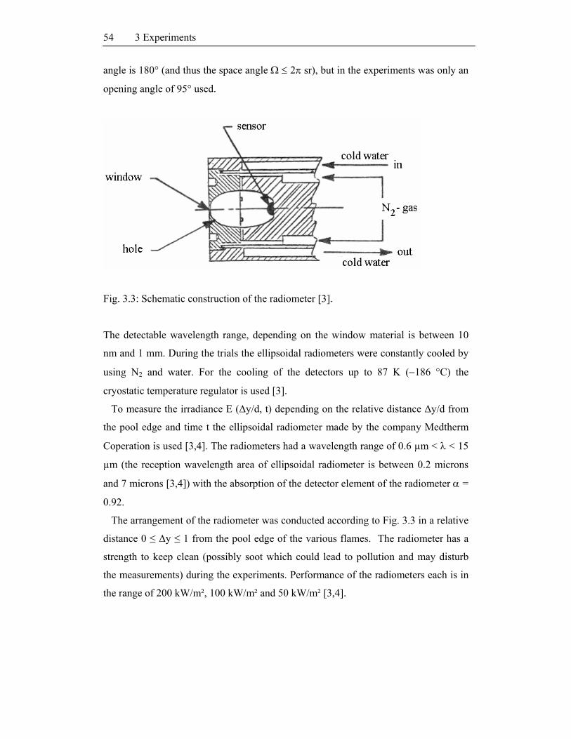
3 Experiments 54
angle is 180° (and thus the space angle 2 sr), but in the experiments was only an
opening angle of 95° used.
Fig. 3.3: Schematic construction of the radiometer [3].
The detectable wavelength range, depending on the window material is between 10
nm and 1 mm. During the trials the ellipsoidal radiometers were constantly cooled by
using N2 and water. For the cooling of the detectors up to 87 K (186 °C) the
cryostatic temperature regulator is used [3].
To measure the irradiance E (Δy/d, t) depending on the relative distance Δy/d from
the pool edge and time t the ellipsoidal radiometer made by the company Medtherm
Coperation is used [3,4]. The radiometers had a wavelength range of 0.6 µm < < 15
µm (the reception wavelength area of ellipsoidal radiometer is between 0.2 microns
and 7 microns [3,4]) with the absorption of the detector element of the radiometer =
0.92.
The arrangement of the radiometer was conducted according to Fig. 3.3 in a relative
distance 0 ≤ Δy ≤ 1 from the pool edge of the various flames. The radiometer has a
strength to keep clean (possibly soot which could lead to pollution and may disturb
the measurements) during the experiments. Performance of the radiometers each is in
the range of 200 kW/m², 100 kW/m² and 50 kW/m² [3,4].

3.6 Wind measurements
55
3.6 Wind measurements
Registration for the wind conditions is done by 10 m high tower with sensor mounted
at heights of 2 m, 6 m and 10 m. The measuring station registered the wind speed and
direction with a time resolution of 3 s [3].

3 Experiments 56

4 Some important topics of CFD used in this work
The numerical fluid mechanics, Computational Fluid Dynamics (CFD) is based on the
solution of the conservation and transport equations for mass, momentum, energy and
mass fractions of various species. In a case of turbulent flows, the Reynolds averaged
transport equation for modeling of turbulence is solved in addition to these equations.
Most commercial CFD codes use finite volume method for solving the above
mentioned equations. Fig. 4.1 shows is the theoretical way to solve a fluid mechanic
problems by CFD simulation e.g. contained in ANSYS CFX and FLUENT softwares.
Fig. 4.1: Procedure of solving fluid mechanic problems by CFD simulation.
4.1 The conservation equations in fire modeling
Combustion processes consist of a variety of processes such as flow, chemical
reaction and molecular transport, for example, heat conduction, diffusion and
radiation. Such a chemically reactive flow can be described at any time and anywhere
by characteristics such as pressure, density, temperature, speed and composition of the
mixture [68]. These sizes vary depending on time and space. Some sizes in these
chemically reactive flows have the property that they are independent of the
processes. These include energy, mass and the momentum.

4 Some important topics of CFD used in this work 58
The mathematical modeling of transport processes is based on conservation
equations.
The basic idea is that the storage of a conservation size in a control volume is equal
to the sum of flows from the volume at the volume surface. Both, the convective as
well as the diffusive flows are covered. Generally, overall conservation equation of
value can be presented as a change in the density function of a general state in
Euler's coordinates:
Φ
SourceConvective DiffusiveAccumulative
ρΦ)ρvΦ D gradΦ S
t
(( ) ( )
. (4.1)
The symbol stands for the nabla operator. In this work the partial differential
equations in the three spatial directions indicate:
x y z, ,
. (4.2)
According to Eq. (4.1) the temporal change of size by the convective and
diffusive transport with the general exchange coefficients D is determined, as well as
through local sources or sinks S. The nature of the sources may be completely
different and depends on the conservation size. Source terms can be temporally and
spatially variable and dependent on one or even several different conservation sizes.
In species conservation equation occur, for example source terms for the change of
species mass fractions as a result of chemical reactions. The simulation of pool flames
needed conservation equations of a reactive gas-soot mixture in the gravity, obtained
by substitution of variable by the following variables:
- mass, = 1 for the continuity equation;
- speed, = u for the momentum conservation equation;
- energy, = E for the energy conservation equation;
- species, = ni for the species conservation equations.
In the following chapter the conservation equations of mass, species, momentum
and energy for a complete description of the interaction between the combustion and
the flow field are presented.

4.1 The conservation equations in fire modeling
59
4.1.1 Overall mass conservation
An essential component of a system is the mass. The mass has no sources inside a
finite volume and in contrast to the molecular species no transportation. For mass
density based on the overall density it follows:
ρρu
t( )
. (4.3)
Eq. (4.1) is also known as continuity equation and is designated for compressible
flows. In the special case of incompressible flows or density dependent flows the
continuity equation is simplified to:
= 0 . (4.4)
Fig. 4.2a: Mass derivation balance in a differential volume element dV = dx1dx2dx3.
In Fig. 4.2a a differential volume element dV = dx1dx2dx3 according to the Eulerian
consideration is shown. The infinitesimal mass dm in the element is given by dm =
ρdV = ρdx1dx2dx3. According to the mass balance, a temporal change of the mass in
flow element in the volume element dV is equal to the difference between a mass
inflow and outflow. In the x1 direction through the area dA1 = dx2dx3 a mass inflow is
m1 and an mass outflow is 1 1 1 1m + m x x( / ) with 1m = ρv1dA = ρv1dx2dx3. The
product ρv1 is mass flow through the unit surface perpendicular to the x1 coordinate
and gives mass flow density. The difference between incoming and exiting mass flow
in x1 direction is:
1 11 1 1 1 1 2 3
1 1
ρv ρvm m x A x x x
x x
) ( )
. (4.5)
The difference between the incoming and exiting mass flows in all three coordinates
and directions divided by dx1dx2dx3, gives the mass balance in volume element dV
written as:

4 Some important topics of CFD used in this work 60
31 2
1 2 3
ρvρv ρvρ
t x x x
( )( ) ( ).
(4.6)
The Eq. (4.6) can be also written as:
ρ(ρv)
t
. (4.7)
This differential mass conservation equation is included in numerical solution of the
flow as continuity equation [83,84]. Since that contains only momentum and
convective term, the mass balance equation is mathematically easier to solve than the
other balance equations.
4.1.2 Species mass conservation
The mass balance equation is based on the total mass of a system. For a system with
more substances in which the distribution of various species of interest is also
connected with chemical reactions and separately accounting of each species is
required. Looking at the mass of various species, the partial density ρi of the ith
component is given by ρv1,α where α = 1,2,3. When the speed of the ith component in a
multi-substance system (or mixture) is defined as the v1,α , with α = 1,2,3, the
summation of all components gives a flux density:
n
i iαi=1
ρv ρ v , α = 1,2,3. (4.8)
The temporal change in the partial mass per unit volume resulted from a partial mass
flow over the border area as well as and the balance from the chemical reactions in the
volume element have formed partial mass. Conservation equations for the partial mass
will be written analogous to the continuity equation for components:
1
i iαi
ρ vρ+ m
t x
( )
. (4.9)
The speed of the ith component consists of the main velocity, vi,α, α = 1,2,3 and the
diffusion speed (ji,α / ρi), α = 1,2,3:
iααiα
i
jv = v +
ρ, α = 1,2,3. (4.10)
It follows the balance equation for ρi:

4.1 The conservation equations in fire modeling
61
α αi ii
α
(ρ v + j )ρ+ m
t x
α = 1,2,3. (4.11)
For example in the software CFX and FLUENT, for accounting of mass fraction
Yi = i /, the following equation is given:
ii i i i
ρYρY u (D ρY ) + S
t
( )
. (4.12)
Based on relationship in Eq. (4.12) for all species i and subsequent summation the
global mass balance equation logically follows that the summation of the source terms
of chemical reactions and the diffusion terms is equal zero. Since all mass Yi breaks
to one sum and the global mass conservation is resolved in any case, the conservation
Eq. (4.12) has to be resolved only for i1 species. The mass fraction of species can be
easily found by difference. Due to relatively small number of balance equations, the
replacement of a partial differential equation by an algebraic relation makes a
substantial reduction of the time.
In the chemical balances, for example dissociation balance, however, the balance of
species must be described by the forward and backward kinetics reaction. Such
reactions have great speed constants, so that the equations for each species are
strongly linked. There is therefore a rigid system of equations whose solution requires
specific mathematical procedures. For such systems the rate constants are not usually
available in the literature and can only be roughly estimated.
4.1.3 Momentum conservation
The temporal change of the momentum density ρvα, α = 1,2,3 can be done by external
forces to the surface of the volume element dV, and by so-called far distance forces or
volume forces to the mass.
The momentum flux density is composed of the convective part α βv ( v ) , α, =
1,2,3 and the part of power density tensor Pα,, = 1,2,3 as shown in Fig. 4.2b. The
convective part of the momentum density in the volume can be written analogous to
the mass conservation:
β β
conv. α
v v v
t x
( ) ( )
. (4.13)

4 Some important topics of CFD used in this work 62
The momentum flux density in the volume element dV by surface forces can be
calculated as:
β αβ αβα α ααβ αβsurf. α α
v P P1P dA P dA dx dA
t dV x x
( )
, = 1,2,3. (4.14)
Here is only the gravitational force g, = 1,2,3, as a mass force for combustion
processes considered. For the mass force in a volume it follows: g, = 1,2,3.
For the momentum equation based on the three above mentioned parts it follows:
ββ αβ β
α
v 1( v v P ρg
t x)
( )
, = 1,2,3. (4.15)
Fig 4.2b: Derivation of momentum balance at a differential volume element dV.
4.1.4 Energy conservation
There are many kinds of energy in a system which can be converted into each other.
The description of the energy requires a higher coupling of the mass and momentum.
In this chapter, the conservation of energy is described by a separate view of kinetic,
potential and the total energy [85].
For example, while in solids, the heat conduction is only process, in fluids with
relatively low temperature the heat transfer by convection is the dominant process. In
reactive flows, such as pool flames, presented in this work, beside the convection,
energy source terms due to chemical reactions and the energy transport due to the heat
radiation are important. An energy conservation equation presented in CFX and
FLUENT software is:

4.1 The conservation equations in fire modeling
63
Ttot
tot hHeat SourceConvectiveWork of conduction termtransport Viscouspressure forces work
ρh p 2(ρuh ) ( T) u + ( u) uδu S
t t 3
)(
(4.16)
where source term can contain chemical reaction or radiation term. Total enthalpy of
the system consists of static and kinetic enthalpy:
2tot stat
1h = h + u
2. (4.17)
The specific static (thermodynamic) energy of the system consists of internal energy
U and the state of the fluid:
statstat
stat
ph = U +
ρ. (4.18)
The temporal change of the energy (Eq. (4.16)) is due to the work of pressure forces
(a), the convective transport (b), the heat conduction (c) and the viscous work (d). In
addition, the source term (s) can include chemical reactions or radiation. For the
energy conservation movement, the total energy source must therefore be free. So, the
source term describes only the transformation of individual forms of energy into each
other, such as the change of inner energy through the heat of chemical reaction
process or the conversion of potential into kinetic energy through work. That is
included in the sub-models described in the Chapter 4.2.
4.2 Sub-models in fire modeling
Mathematical modeling is the image of the resulting physical and chemical processes
caused by states or state changes in a system, described with the help of mathematical
relationships. Often, these equations due to their complexity can not be solved
analytically, so the numerical solution methods are needed. The first step is a spatial
discretization of grid structures in finite elements or subdivided volumes. The solution
of the balance equations can be done at the discrete nodes using arithmetic operations.
They have iterative methods, in which the solution is gradually approximated. The
individual steps are repeated, the results of a run as the starting values for the next
step are used. This approach requires defined start values for the first step and also
defines the boundary conditions of the investigated area.

4 Some important topics of CFD used in this work 64
The exact solution of the conservation equations requires resolution of the smallest
occurring length and time scales. The smallest scale is Kolmogorov [78]. For the
special case of fully developed isotropic turbulence, Kolmogorov derived that the
relation: e(k) k5/3 is valid for completely developed turbulence [68]. To resolve the
smallest scale a Direct Numeric Simulation (DNS) should be used. For a typical
turbulent flow with Rl = 500, a l0/lk = 100, thus, about 1000 grid points in one
dimension are needed, 109 grid points in three dimension to resolve the smallest
turbulence eddies. The Navier-Stokes equation is time dependent so at least 1000 time
steps are needed to mimic a turbulent combustion process, the number of
computational operations exceeds 1014 [68].
The demands on the memory and computing power, even by use of modern parallel
computers of the near future can not be fulfilled. So, direct numerical simulations for
the most technically relevant systems are currently not yet feasible and introduction of
simplified models are needed. The simplifications contained therein can give a
possible good description of certain physical or chemical processes without their
direct calculation and thus reduce the computational effort. Different models with
various complexity and accuracy for the most important problems such as the
treatment of turbulence, heat radiation and soot formation have been developed.
Numerical simulations are often an ideal support to the experiments due to the
opportunities to calculate situations which can not be obtained experimentally or are
difficult to obtain. In experiments, in contrary to CFD the many sizes are often only
selectively measured, in part, there are areas where for example measurements are not
possible due to the geometric or the safety reasons. CFD offer many of possibilities,
e.g. in modified various boundary or geometries and has ability to calculate all sizes
such as velocities, temperatures and concentrations of all the species in the entire
recorded territory.
In this work, the software packages ANSYS CFX and mesh generator ICEM CFD
are used as well as the ANSYS FLUENT and its mesh generator GAMBIT. The
programs are based on Euler's view of the fluid. This means that the macroscopic
change of state variables is registered at a fixed location or in a fixed control volume
[82]. In contrast, the microscopic Lagrangian representation of the movement of a
particle through a system is prosecuted. Basically, a combination of the two possible

4.2 Sub-models in fire modeling
65
methods is possible, such as the simulation of the combustion of coal particles in fire
or burners where the coal particles are with the Lagrange method pursued and the
flame gases with the Euler method described. In all of the control volumes produced
by discretization, partial calculations are carried out and resulted calculation steps are
used to hold with balance sizes. The assumptions and simplifications of the individual
models and the resulting calculation steps are described in subsequent chapters.
4.2.1 Modeling of turbulence
In principle, a flow can be characterized as laminar or turbulent, with a smooth
transition between two states. Laminar flows are characterized by parallel flow lines
in the main flow direction. Disorders are relatively quickly restored and the initial
flow conditions recovered. In contrast, in turbulent flows occur eddies, which by
disturbances such as shear walls between impulse and fluid or fluid exchange between
layers rise with different speeds. The vortex effect increases transportation of all sizes
across the balance sheet or contrary to the main flow direction. The flow through the
eddy formation is irregular, chaotic and difficult to predict. The transition from
laminar to turbulent flow occurs at a characteristic Reynolds number
ρul ulRe = =
μ v (4.19)
with the density and a dynamic viscosity μ or a kinematics viscosity v. Furthermore,
for one system the characteristic speed u and a characteristic length l must be
determined. Thus, for example, in tube flows where l is usually equal to the pipe
diameter, the transition point from laminar to turbulent flow is then at Re 2000. In
turbulent flows carried by momentum and energy exchange between the vortices a
decay of larger vortices to smaller is happening. Here, the turbulence energy will
transfer to internal or thermal energy. The largest length scales correspond to the
geometric dimensions of the system, so-called integral length l0. Through the steady
decay a cascade of energy are created, which ends with the smallest measured,
Kolmogorov length lk. By the Kolmogorov length is the kinetic energy of small
vortices so dissipated that the half time of rotation of one vortex is equal to the time
for the diffusion along the diameter lk. Thus, under the lk the diffusion is faster than
the turbulent transport and turbulent processes can no longer occur. The distribution
of turbulent kinetic energy to the different length scales may be determined from the

4 Some important topics of CFD used in this work 66
spectral energy density e(ke). It is partly dependent on the wave number ke, which is
equal to the reciprocal of the turbulent length l. It is linked with the average specific
turbulent kinetic energy per unit mass q as follows [86]:
0e eq(r, t) e(k , r, t)dk
= . (4.20)
Fig. 4.3: Turbulent energy spectrum: l0 symbolizes the integral length, lk,a, lk,b, lk,c
which are the Kolmogorov-length dimensions for three Reynolds numbers a = Re1 < b
= Re2 < c = Re3 [80].
The logarithmic application in Fig. 4.3 shows that in a three-dimensional flow the
spectral energy density declines at smaller length scales proportionally to ke–5/3. This
means that the main part of turbulent kinetic energy in located in the large vortices.
The influence of the Reynolds numbers on the spectral energy density is based on the
three curves: a, b and c. With increasing Reynolds number from curve a to curve c
moves the Kolmogorov length to smaller wavelengths, i.e. here the turbulence
dominates in transport of increasing number of smaller vortices. To describe the
turbulence degree a geometry dependent Reynolds number and turbulent Reynolds
number can be used [86]:
0l
ρ 2qlR =
μ. (4.21)
The Kolmogorov length can be calculated by the turbulence Reynolds number:
03/4kl
ll =
R. (4.22)

4.2 Sub-models in fire modeling
67
Due to the ongoing conversion of kinetic energy in the internal or thermal energy
turbulent flows require a permanent supply of power for its maintenance. This may be
caused, for example, by a constant flow based on gravitational forces, in nature or in
the pipeline by pumping effect. The spatial discretization of very small length scales
of the smallest vortices and thus the direct numerical calculation in practical
applications with today's computer technology is not possible. Therefore, the
turbulence without their exact resolution use certain assumptions described below.
Some of the most commonly used models for turbulence modeling will be described
below.
4.2.1.1 k-ε and k-ω models
Generally, turbulence model is presented by a partial differential equation. Contains
the equation new unknown, such as a turbulent dissipation ε(x, y), a further modeling
of equations is possible. Depending on how many partial differential equations are
used there exist one-equation models, two-equation models, etc. The k-ε turbulence
model is a two-equation model. Two-equation models k-ε and k-ω use the gradient
diffusion hypothesis to relate the Reynolds stresses to the mean velocity gradients and
the turbulent viscosity. The turbulent viscosity is modelled as the product of a
turbulent velocity and turbulent length scale. Both the velocity and length scale are
solved using separate transport equations (hence the term 'two-equation'). In two-
equation models, the turbulence velocity scale is computed from the turbulent kinetic
energy, which is provided from the solution of its transport equation. The turbulent
length scale is estimated from two properties of the turbulence field, usually the
turbulent kinetic energy and its dissipation rate. The dissipation rate of the turbulent
kinetic energy is provided from the solution of its transport equation [83,84]. The
model describes two partial differential equations for development of the turbulent
kinetic energy i iu uk =
2
defined as the variance of the fluctuations in velocity and ε
the turbulence eddy dissipation (the rate at which the velocity fluctuations dissipate)
k
uε = v
x
2
[83,87].
The equation of k-ε turbulence model with kinetic energy k is given by the following
relations:

4 Some important topics of CFD used in this work 68
j titj
j j i k j
uu μk k kρ ρu = c ρμ ρε +
t x x x x xj
, (4.23)
2 2ji i i
μ tε1 ε2 ε2j i, jj j j i j
uu u uε ε ερ ρu = c τ c c ρμ c ρ +
t x k x k x x x k
t
εj j
μμ +
x σ x
. (4.24)
In the above equations are few, simplified model assumptions incorporated. This
restricts the scope of equations. In these equations appear still unknown coefficients.
These are supplemented by the consideration of simple flow fields. The parameter cε1
is calibrated by a homogeneous shear train at equilibrium. The size cε2 follows from
the decay of homogeneous grid turbulence. The turbulent Prandl number σε is derived
from an analysis of the logarithmic area of a wall turbulent boundary layer. From the
context of the anisotropic parameter cμ the eddy viscosity can be averaged to νt = cμ
(k²/ε). For the turbulent boundary a value for cμ is used. For the standard k-ε model, in
the literature the following constants can be found:
cμ = 0.09, cε1 = 1.44, cε2 = 1.92, σε = 1.3, σk = 1.
The standard k-ε turbulence model is characterized by its numerical stability and
especially relatively small computing time and is easy to implement. Within ANSYS
CFX and FLUENT, the k-ε turbulence model with buoyancy terms is available with
the scalable wall-function approach added to improve robustness and accuracy when
the near-wall mesh is very fine. If the full buoyancy model is being used, the
buoyancy production term is modelled as:
tkb
ρ
μP = g ρ
ρσ . (4.25)
This buoyancy production term is included in the k and ε equation if the buoyancy
turbulence option is set as an option [83,84].
4.2.1.2 Large Eddy Simulations
Large Eddy Simulation (LES) presents a completely different approach in calculating
turbulence as the Reynolds averaged models and allows a much more accurate
description of a turbulent flow field. Turbulent flows include a variety of eddies,
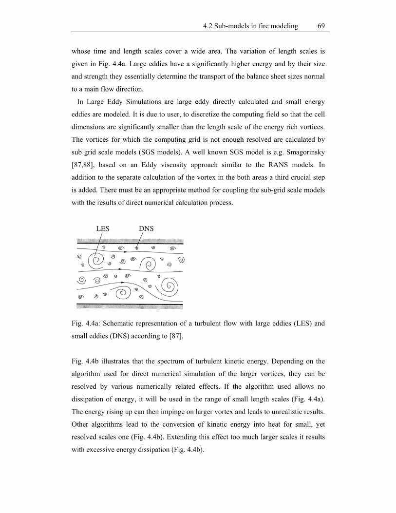
4.2 Sub-models in fire modeling
69
whose time and length scales cover a wide area. The variation of length scales is
given in Fig. 4.4a. Large eddies have a significantly higher energy and by their size
and strength they essentially determine the transport of the balance sheet sizes normal
to a main flow direction.
In Large Eddy Simulations are large eddy directly calculated and small energy
eddies are modeled. It is due to user, to discretize the computing field so that the cell
dimensions are significantly smaller than the length scale of the energy rich vortices.
The vortices for which the computing grid is not enough resolved are calculated by
sub grid scale models (SGS models). A well known SGS model is e.g. Smagorinsky
[87,88], based on an Eddy viscosity approach similar to the RANS models. In
addition to the separate calculation of the vortex in the both areas a third crucial step
is added. There must be an appropriate method for coupling the sub-grid scale models
with the results of direct numerical calculation process.
Fig. 4.4a: Schematic representation of a turbulent flow with large eddies (LES) and
small eddies (DNS) according to [87].
Fig. 4.4b illustrates that the spectrum of turbulent kinetic energy. Depending on the
algorithm used for direct numerical simulation of the larger vortices, they can be
resolved by various numerically related effects. If the algorithm used allows no
dissipation of energy, it will be used in the range of small length scales (Fig. 4.4a).
The energy rising up can then impinge on larger vortex and leads to unrealistic results.
Other algorithms lead to the conversion of kinetic energy into heat for small, yet
resolved scales one (Fig. 4.4b). Extending this effect too much larger scales it results
with excessive energy dissipation (Fig. 4.4b).

4 Some important topics of CFD used in this work 70
Fig. 4.4b: Influence of different algorithms on the calculated turbulent energy
spectrum [80]: (a) the algorithm is to diffusive (b) MILES algorithm, (c) the algorithm
blocks the energy dissipation.
To solve a problem in the transition between resolved and modeled scales to a Large
Eddy Simulations filtering features are introduced. They suppress the unwanted
numerical effect on the cut off of the grid; on the other hand, they serve as a basis for
describing the transport processes beneath the grid size. Conventional LES does not
solve the Navier-Stokes equations directly, but a secondary through a set of equations
for filtered sizes. So, the balance size Ф consists of a large part numerically
resolved and a small, non-resolved part Ф' [80]:
Ф = + Ф'. (4.26)
The resolution is part of volume averaging, taking into account the filter function G
[80]:
V
Φ(x, y, z) = G(x x , y y , z z )Φ(x , y , z , t)dx´dy´dz´ . (4.27)
As a filter function, for example, top-hat filter or Gaussian filter can be used. The cell
width below which the eddy is no longer resolved a user can chose freely. In general,
for Large Eddy Simulation, however, a much finer time and space discretisation is
required than for RANS modeling. As a maximum time step size can be a value of t =
104 s [83]. The calculation of the temporal evolution of a particular size in a certain
time interval of at least ttot = 20 s is, however, with the current state of computer
technology extremely time consuming. Large Eddy Simulations need boundary layers
in an extremely fine grid. Therefore, the combinations of LES and unsteady RANS
4.2 Sub-models in fire modeling
71
(URANS) are designed to work on this problem. In the so called Scale Adaptive
Simulation [83] is depending on the size of cells where LES switches to URANS.
Ideally, the transient, anisotropic turbulence in the border areas through layers
detached LES is directly calculated. The boundary layers are, however, with URANS
models simulated. This allows the computing time to be significantly reduced.
However, the results are dependent directly from the grid, the transfer point of the
vortex from the boundary layer can with an inappropriate cell sizes be negatively
affected.
Turbulent flows are characterized by eddies with a wide range of length and time
scales.
The largest eddies are typically comparable in size to the characteristic length of the
mean flow. The smallest scales are responsible for the dissipation of turbulence
kinetic energy. It is possible, in theory, to directly resolve the whole spectrum of
turbulent scales using an approach known as direct numerical simulation (DNS). No
modeling is required in DNS. However, DNS is not feasible for practical engineering
problems involving high Reynolds number flows. The cost required for DNS to
resolve the entire range of scales is proportional to 3tRe , where Ret is the turbulent
Reynolds number. Clearly, for high Reynolds numbers, the cost becomes prohibitive.
In LES, large eddies are resolved directly, while small eddies are modeled. Large
eddy simulation (LES) thus falls between DNS and RANS in terms of the fraction of
the resolved scales. The rationale of LES can be summarized as follows:
- Momentum, mass, energy, and other passive scalars are transported mostly by large
eddies.
- Large eddies are more problem-dependent. They are dictated by the geometries and
boundary conditions of the flow involved.
- Small eddies are less dependent on the geometry, tend to be more isotropic, and are
consequently more universal.
- The chance of finding a universal turbulence model is much higher for small eddies.
Resolving only the large eddies allows one to use much coarser mesh and larger
times step sizes in LES than in DNS. However, LES still requires substantially finer
meshes than those typically used for RANS calculations. In addition, LES has to be
run for a sufficiently long flow-time to obtain stable statistics of the flow being
modeled. As a result, the computational cost involved with LES is normally orders of

4 Some important topics of CFD used in this work 72
magnitudes higher than that for steady RANS calculations in terms of memory
(RAM) and CPU time. Therefore, high-performance computing (e.g., parallel
computing) is a necessity for LES, especially for industrial applications. The
following text gives details of the governing equations for LES, the sub-grid scale
turbulence models, and the boundary conditions.
The governing equations employed for LES are obtained by filtering the time-
dependent Navier-Stokes equations in either Fourier (wave-number) space or
configuration (physical) space. The filtering process effectively filters out the eddies
which scales are smaller than the filter width or grid spacing used in the computations.
The resulting equations thus govern the dynamics of large eddies.
A filtered variable (denoted by an over bar) is defined by
D
j(x) = j(x )G(x, x )dx (4.28)
where D is the fluid domain, and G is the filter function that determines the scale of
the resolved eddies. The finite-volume discretization itself implicitly provides the
filtering operation:
v
1j(x) = j(x )dx , x v
V (4.29)
where V is the volume of a computational cell. The filter function, G(x, x ) , implied
here is then
1 / V, x v,G(x, x )
0, x othervise
(4.30)
The LES capability is applicable to compressible flows. For the sake of concise
notation, however, the theory is presented here for incompressible flows.
Filtering the Navier-Stokes equations, one obtains
ii
ρ ρ(ρu ) = 0
t x
(4.31)
and
ij iji i j
i j j j
σ τρ ρ ρ p(ρu ) (ρu u )
t x x x x xi
( )
(4.32)
where ijσ is the stress tensor due to molecular viscosity defined by

4.2 Sub-models in fire modeling
73
ji iij ij
j i i
uu u2σ μ δ
x x 3 x
(4.33)
and ijτ is the sub-grid scale stress defined by
ij i j i jτ ρu u ρu u . (4.34)
The sub-grid scale stresses resulting from the filtering operation are unknown, and
require modeling. The sub-grid scale turbulence models in CFX and FLUENT employ
the Boussinesq hypothesis [83] as in the RANS models, computing sub-grid scale
turbulent stresses from
tij kk ij ij1
τ τ δ 2μ S3
(4.35)
where t is the sub-grid scale turbulent viscosity. The isotropic part of the sub-grid
scale stresses kkτ is not modeled, but added to the filtered static pressure term. ijS is
the rate of strain tensor for the resolved scale defined by
jiij
j i
uu1S
2 x x
. (4.36)
For compressible flows, it is convenient to introduce the density-weighted (or Favre)
filtering operator:
ρ
ρ
. (4.37)
A further detail in defining the coefficients can be found in [84].
The dynamic Smagorinsky-Lilly model is used in this work. Here, a sub-grid scale
turbulent flux of a scalar, , is modeled using s sub-grid scale turbulent Prandtl
number by
tj
t j
μq =
σ x
(4.38)
where qj is the sub-grid scale flux.
Germano et al. [84] and subsequently Lilly [84] conceived a procedure in which the
Smagorinsky model constant, Cs, is dynamically computed based on the information
provided by the resolved scales of motion. The dynamic procedure thus obviates the
need for users to specify the model constant Cs in advance. The details of the model

4 Some important topics of CFD used in this work 74
implementation in FLUENT and its validation can be found in [84]. The Cs obtained
using the dynamic Smagorinsky-Lilly model varies in time and space over a fairly
wide range. To avoid numerical instability, Cs is clipped at zero and 0.23 by default.
4.2.1.3 Scale Adaptive Simulations
SAS [83,89] is a hybrid model contains the Unsteady Reynolds Averaged Navier
Stokes Equation (URANS) and the Large Eddy Simulation (LES), where URANS
acts in the near of wall boundaries and LES in the remaining part of the domain. SAS
is an improved URANS formulation, which allows the resolution of the turbulent
spectrum in unstable flow conditions. SAS model dynamically adjusts to resolved
structures in a URANS simulation, which results in a LES-like behavior in unsteady
regions of the flow field. At the same time, the model provides standard RANS
capabilities in stable flow regions.
Scale-Adaptive Simulation (SAS) allows the simulation of unsteady flows with both
RANS and LES content in a single model environment. As SAS formulations use the
von Karman length scale as a second external scale, they can automatically adjust to
resolved features in the flow. As a result, SAS develops LES like solutions in
unsteady regions, without a resort to the local grid spacing.
The concept of Scale-Adaptive Simulation (SAS) [83,89] allows the simulation of
unsteady turbulent flows without the limitations of most Unsteady RANS (URANS)
models. Contrary to standard URANS, SAS provides two independent scales to the
source terms of the underlying two-equation model. In addition to the standard input
in form of the velocity gradient tensor, ∂ui/∂xj , SAS models compute a second scale
from the second derivative of the velocity field. The resulting length scale is the well
known von Karman length scale LvK. The introduction of LvK allows the model to
react more dynamically to resolved scales in the flow field which cannot be handled
by standard URANS models. As a result, SAS offers a single framework, which
covers steady state RANS as well as LES regions, without an explicit switch in the
model formulation. SAS therefore offers an attractive framework for many “multi-
scale” flow problems encountered in industrial CFD. It provides a steady state (or
mildly unsteady) solution in stable flow regions (like boundary layers), and unsteady
structures in unsteady regions within a single model framework. SAS allows a
4.2 Sub-models in fire modeling
75
breakdown of the large unsteady structures by adapting the turbulence model to the
locally grid spacing [83,89].
The SAS approach represents a new class of the URANS models. Different from the
conventional RANS formulations, the SAS model adjusts the turbulence length scale
to the local flow inhomogeneities. As a measure of the local flow length scale, a
classic boundary layer length scale introduced by von Karman κU′(y)/U′′(y) is
generalized for arbitrary three-dimensional flows. The von Karman length scale
explicitly enters the transport equations of the turbulence model. The resulting model
remains a RANS model, as it delivers proper RANS solutions for stationary flows and
maintains these solutions through grid refinement. On the other hand, for flows with
transient instabilities like those in the massive separation zones, the model reduces its
Eddy viscosity according to the locally resolved vortex size represented by the von
Karman length scale. The SAS model can under those conditions resolve the turbulent
spectrum down to the grid limit and avoids RANS-typical single-mode vortex
structure.
1. SAS modeling is based on the use of a second mechanical scale in the source/sink
terms of the underlying turbulence model. In addition to the standard input from the
momentum equations in the form of first velocity gradients (strain rate tensor,
vorticity tensor) SAS models rely on a second scale, in the form of higher velocity
gradients (typically second derivatives).
2. SAS models satisfy the following requirements:
a. Provides proper RANS performance in stable flow regions.
b. Allows the break-up of large unsteady structures into a turbulent spectrum.
c. Provides proper damping of resolved turbulence at the high wave number
end of the spectrum (resolution limit of the grid).
3. Functions (2a) and (2b) are achieved without an explicit grid or time step
dependency in the model. Naturally, function (2c) has to be based on information on
the grid spacing, other information concerning the resolution limit (dynamic LES
model, etc.), or the numerical method (MILES damping etc.)
A complete description of the SST-SAS model will be published elsewhere due to
space limitations. A compressed model formulation is provided here to leave more
space for the test case results. The governing equations of the SST-SAS model differ

4 Some important topics of CFD used in this work 76
from those of the SST RANS model by the additional SAS source term QSAS in the
transport equation for the turbulence eddy frequency ω (Eq. 4.39a,b):
tμk
k
μρk)(ρUk) = P ρc kω + μ + k
t σ
(
(4.39a)
SAS2 t
1kω ω2
μρ ω 2ρ 1(ρUω) = α P ρβω + Q + μ + ω + (1 F ) k
t k σ σ ω
( )
(4.39b)
where σω2 is the σω value for the k-ε regime of the SST model.
SASK
2 2 22
2 2L 2ρk k
Q = max ρξ κS C max 0L σ k2
| | | |, ,
. (4.40)
More details about coefficients used in equations included in SAS model can be found
in [83,89].
Adaptive scale simulation (SAS) model is advanced URANS (unsteady RANS)
model which allows a realistic calculation of unsteady flows. Unlike standard
URANS methods, which typically resolve only large scale structures, SAS allows a
greater turbulence decay elements in a turbulent spectrum. SAS reaches the transient
improvement in the field by taking into account the Karman length scale in the scaling
of the equation turbulence model. This allows the model already resolved structures
and avoids the smearing which is typical in the standard URANS methods. A detailed
mathematical description can be found in CFX guideline [83].
4.2.2 Combustion models
4.2.2.1 Source terms of species on the basis of chemical reactions
In reactive flows for i1 species for each species will one balance equation Eq. (4.12)
be solved (Section 4.1.2). The changes of the species mass fractions Yi due to
chemical reactions are considered in a source term Si. It follows for all first reactions
with all species with the stoichiometric coefficients i,rv , and i,rv of the species i on the
reaction or product side in the reaction r:

4.2 Sub-models in fire modeling
77
N NS S
i =A,B,C,... i=A,B,C,..i,r i,rv i v
.
. (4.41)
The source Si, used to increase or decrease the mass fraction of a contributed species,
is calculated as a sum of the changes due to all reactions:
NS
i =A,B,C,..ri i i,r i,rS = M v v R
.
( ) . (4.42)
The reaction speed Rr can be calculated by using different models, for example, with
an Eddy Break Up model [68,83], the Eddy Dissipation model [68,83] or a Finite Rate
Chemistry model [83]. As a main part of this work is the modeling of combustion of
JP-4 (jet propulsion) fuel. The chemical reactions for combustion of JP-4 fuel are
calculated with three different approaches: multistep chemical reaction and two
different flamelet models: the Laminar flamelet model with pdf, with 112 species and
800 chemical reactions and Pdf transport model for species with 20 species and 40
chemical reactions (Section 4.4.3.2).
4.2.2.2 The Eddy Dissipation Model
The Eddy dissipation model is based on the concept that chemical reaction is fast
relative to the transport processes in the flow. When reactants mix at the molecular
level, they instantaneously form products. The model assumes that the reaction rate
may be related directly to the time required to mix reactants at the molecular level. In
turbulent flows, this mixing time is dominated by the eddy properties and, therefore,
the rate is proportional to a mixing time defined by the turbulent kinetic energy, k, and
dissipation, ε.
Rate ε
k . (4.43)
This concept of reaction control is applicable in many industrial combustion problems
where reaction rates are fast compared to reactant mixing rates. In the Eddy
Dissipation model, the rate of progress of elementary reaction k, is determined by the
smallest of the two following expressions:
Reactants limiter: kkI
ε c(I)R = A min
k ν
(4.44)
where c(I) is the molar concentration of component I and I only includes the reactant

4 Some important topics of CFD used in this work 78
components.
Product limiter: P
P
I
kIkI
c(I)Wε
R = ABk ν W
(4.45)
where P loops over all product components in the elementary reaction k.
Details can be found in [83].
4.2.2.3 Flamelet model
Non-premixed flame is characterized in general by a diffusive transportation of fuel
and oxidizer through the flame zone, which is slow compared to the chemical reaction
[68,83,90]. If the molecular mixture occurs below the level of the smallest vortices,
the combustion takes place then at the surface of theoretically infinite thin layers, and
layers are smaller than the Kolmogorov length. These one dimensional, laminar flame
fronts will hence refer to flamelets. The influence of turbulence, expressed in the
folding and stretching of the flamelets from the chemical structure is however not
affected. Because of that the mixture process strongly depends on the diffusion, it is
easier to describe what happens by using a particular diffusion coefficient for each
scalar. Then runs the mixture of all species equally fast, so only a single variable in
the mixture is pursued. As chemical species are formed or consumed in reactions, it is
easier to consider the elements which mass fractions remain unchanged. So, in a two
stream system of the mixture fraction with mass fractions Z of element j it follows
[68,83]:
j j,2
j,1 j,2
Z Z=
Z Z
(4.46)
with Z defined as
NS
i=1
i, j jj i
i
a MZ = Y
M (4.47)
and the molar masses M and mass fractions Y of the species i. The indices 1 and 2
refer to the material flow. Due to that by definition all the diffusion coefficients are
equal; there are no changes in the two streams in the relationship between the
elements. It is easy to show that the mass fraction regardless to the considered element
is [68]:

4.2 Sub-models in fire modeling
79
ξ1 = ξ2 = ... = ξNs. (4.48)
Boundary conditions applies ξ = 1 in the fuel stream and ξ = 0 in oxidant stream. The
mixture fraction can as the mass fraction of the material, be interpreted as the stream
1. The mixture fraction of material in a stream 2 is than 1 – ξ. After summation of all
species equations the equation for the mass fraction is obtained [68,83]:
ρρ ρD
t
( )( ) ( )
. (4.49)
The mass fraction is independent of the chemical reactions, because it refers to
chemical elements, which are not consumed or formed by chemical reactions. Since
the balance equation does not contain a source term, ξ is also as scalar conserved
scalar [83]. Accounting to that the ratio of material to heat transport can be predicted
in connection to the Lewis number
P
λLe =
ρc D (4.50)
which is equal to 1 in the system without heat loses. To describe the situation on one
plane a stoichiometric composition ξ = ξst will a new, locally defined coordinate
system introduce with coordinates x2 and x3 within the reaction zone. The x1
coordinate is perpendicular to the reaction zone and can be defined under the
assumption that these infinite thin zone is presented through the mixture ξ [83,90].
Therefore, the following transformation leads to:
tt
, (4.51)
1 1x x
, (4.52)
k k kx x
. (4.53)
One example is calculation of temperature transformation. For the temperature
equation e.g. in ANSYS CFX follows [83]:
R
k=1 P P P
rk
α kα α α
Q qT T T 1 pρ + ρu ρD ω + +
t x x x c c c t
. (4.54)
The three terms on the right side represent chemical reactions, the radiation and the
transient pressure. The latest effect with rapid pressure changes such as piston
engines. Since the flamelets are very thin, only the gradient normal to the surface of

4 Some important topics of CFD used in this work 80
the stoichiometric mixture has great values. This is taken into account in the terms,
the second derivative in relation to the mixture fraction ξ are neglected to simplify the
equation [83]:
NSR
i=1P P P
2st
i i2
χ qT T 1 1 p+ h m + +
t 2 ρc c c t
. (4.55)
One important parameter in Eq. (4.55) is scale dissipation rate which represents an
influence of the flow field to the reaction zone and it is given by
χ"2ε
= C ξk
. (4.56)
The reaction zone is determined by the flow field stretched by diffusion. At a critical
scalar dissipation crχ is the reaction zone so thin that the heat loss through conduction
can not longer be compensated. The temperatures decrease strongly, locally and the
flame is extinguished at this point. This is of great importance, because this parameter
is ensured that a turbulent flame can be described by an ensemble of one dimensional
flame. The scalar dissipation stχ and the pressure p are flamelet parameters [90]. That
the influences of turbulence in Flamelet model can be taken into account a two
balance equations are needed. The first is required for the Favre averaged mixture
fraction [83,84]:
t
ξ
μρξ)(ρuξ) μ +
t σ
(
. (4.57)
The two additional terms represent the production and dissipation of the variance
term. The dissipation is included in CFX by the empirical correlation:
"2χε
χ = C ξk
. (4.58)
with the constants ξ = ξ''2 = 0.9, Cχ = 2.0. Favre averaged composition of the fluid is a
function of Favre averaged mixture fraction, its variance and the scalar dissipation
rate:
st
1"2
"2ξ,ξ0
i i iY = Y (ξ,ξ ,χ) = Y (ξ,χ )P (ξ) . (4.59)
The function P is a probability density function (pdf). It is used in the statistical
description of the flames properties. The probability density function pdf of a fluid
gives the probability that the fluid in a location r have a density between ρ and ρ+dρ, a

4.2 Sub-models in fire modeling
81
speed in x direction between ux and ux + dux, in y direction between uy and uy + uy
and in z direction between uz and uz + duz, a temperature in the range between T and
T + dT and local mass fractions between Yi and Yi + dYi [68]:
1 N 1 1 N 1S Sx y z x y zP(ρ, u , u ,u , Y ,...., Y ,T; r)dρdu du du dY ,....,dY ,dT
. (4.60)
The probability density function used in this work is based on empirical data. In this
way a statistical independence of each variable is adopted regard to the pdf of one
variable. In this way, the multidimensional pdf is formulated as one dimensional pdf
[68]:
1 N 1 1 N 1S Sx y z x y zP(ρ, u , u , u ,Y ,....,Y ,T; r) P(ρ)P(u )P(u )P(u )P(Y ),...., P(Y )P(T)
.
(4.61)
As individual variables are not independent of each other, additional correlations
between them are introduced. The other one dimensional pdf from experiments is
used to determine which the crucial advantage in the above separation lies.
Fig. 4.5 shows an example a schematic representation of probability density
functions for the mass fraction of the fuel mixture in a turbulent layer, such as on the
edge of a pool of flame can occur. On the edge of the mixing layer is the probability
to find a pure fuel or a pure air relatively high. Within the mixing process, the
probability to found, one of the two components unmixed, is getting lower.
Nevertheless, for a fixed locations pdf one of the two components unmixed to be
found is equal to zero, because of fluctuations the local limits of the reaction zones are
always shifting. For analytical description of such one dimensional pdf different
application functions such as Gaussian function or β-function can be used. By
inserting the mixture fraction can with the help of the β-function Eq. (4.59) be
integrated. The implementation of this calculation step in each cell, for the each
iteration will make a substantial computational effort. Therefore, the concept of look-
up table was introduced. With this approach a preprocessor will make integration
depending on the mixture fracture. For the various mixture fractions resulting
densities, velocities, temperatures and concentrations of species are contained in the
so-called look-up table, so that during the actual simulation the compute-intensive
integration is avoided. Instead, the corresponding values for the flow field and
calculated mixture fraction are readable directly from the table. Through these savings
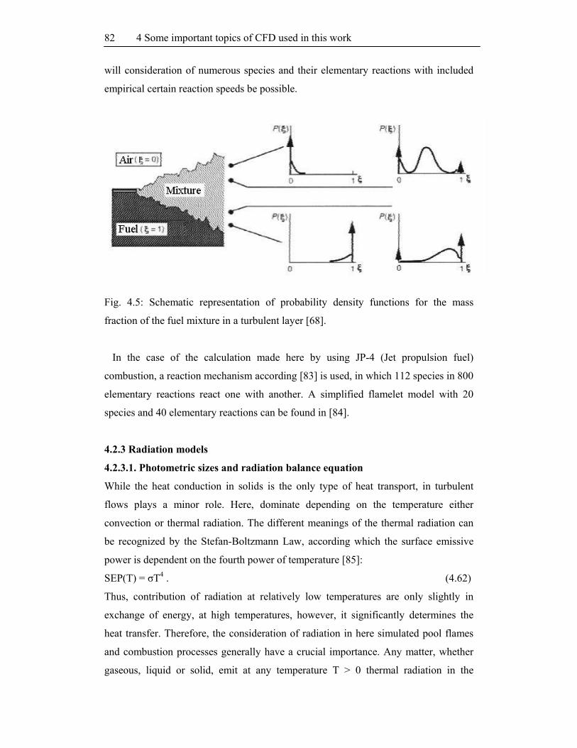
4 Some important topics of CFD used in this work 82
will consideration of numerous species and their elementary reactions with included
empirical certain reaction speeds be possible.
Fig. 4.5: Schematic representation of probability density functions for the mass
fraction of the fuel mixture in a turbulent layer [68].
In the case of the calculation made here by using JP-4 (Jet propulsion fuel)
combustion, a reaction mechanism according [83] is used, in which 112 species in 800
elementary reactions react one with another. A simplified flamelet model with 20
species and 40 elementary reactions can be found in [84].
4.2.3 Radiation models
4.2.3.1. Photometric sizes and radiation balance equation
While the heat conduction in solids is the only type of heat transport, in turbulent
flows plays a minor role. Here, dominate depending on the temperature either
convection or thermal radiation. The different meanings of the thermal radiation can
be recognized by the Stefan-Boltzmann Law, according which the surface emissive
power is dependent on the fourth power of temperature [85]:
SEP(T) = σT4 . (4.62)
Thus, contribution of radiation at relatively low temperatures are only slightly in
exchange of energy, at high temperatures, however, it significantly determines the
heat transfer. Therefore, the consideration of radiation in here simulated pool flames
and combustion processes generally have a crucial importance. Any matter, whether
gaseous, liquid or solid, emit at any temperature T > 0 thermal radiation in the

4.2 Sub-models in fire modeling
83
wavelength range of 0.1 ηm ≤ λ ≤ 100 ηm. The visible wavelength range makes only
a small part of the total energy, the largest part is emitted in the infrared range (Fig.
4.6).
Fig. 4.6: Spectral radiance distribution of a black radiator [85].
Incidence of photons in fluids or solids can produce different effects. By absorption of
a photon its energy is transferred to the fluid or solid. Gases show unlike solids due to
their different transitions discrete energy absorption and emission spectra. The atoms
of a gas are electronically driven, quantized states, in molecules exist discrete
vibration and rotation states. Accordingly, absorption and emission of a gas are
strongly wavelength dependent. In contrast, usually it is assumed that the radiant
energy of impermeable body depends only on temperature and physical characteristics
of the body. Their emission spectrum is independent on the wavelength of the incident
radiation. This assumption is based on the fact that usually the entire radiation energy
absorbed is converted to the internal energy with an equilibrium distribution. Besides
that absorption and emission can still take a place. Famous examples include the
scattering of particles such as dust clouds or liquid droplets in mist. Collisions are

4 Some important topics of CFD used in this work 84
scattering of photons with other particles, where the photons are diverted. During
clashes elastic energy remains unchanged, at inelastic collisions; however, the energy
is usually reduced. If the scattering is direction preferred, it is an anisotropic
scattering. In an isotropic scattering a uniform distribution of the scattered photons
occurs. To describe the radiation the radiometry various sizes are defined. The
accounting of the radiation is usually based on the radiance L. It is defined as the
radiant flux Фrad that in an differential wavelength range dλ projected in direction
from the vertical to ,φ, emits a radiant surface element dAP = dA1cos in the space
angle [85]:
1 1
3radd dI(λ)
L(r,s,λ) =dA cos dΩdλ dA cos
(4.63)
I is called here radiant intensity. The geometric relationships are illustrated in Fig. 4.7.
The radiation flux Фrad is defined as
raddQ
=dt
(4.64)
with that by photon transported radiation energy Q. The product of the absolute
temperature of a black body T and wavelength λmax of maximum surface emissive
power is constant and gives the Wien's displacement law [85]:
λmax T = C2/4.97 = 2.898 . 10–3 mK. (4.65)
Fig. 4.7: Definition of radiance by geometric means [85].

4.2 Sub-models in fire modeling
85
The balance equation for the radiance is taking into account the possible effects
[83,85]:
λ
λ S,λ λscat,λ
abs,λ scat,λ abs,λ
kdL (r,s) = (k + k )L (r,s) + k L (r, s,T) + dL (r,s)ψ(s, s ,Ω)dΩ
4π weighted entered radiatweakening due to blackbody absorption and radiation scattering
Lλ+ S
heat ionsources
(4.66)
Accordingly, the amendment of the spectral radiance along the beam path l at the
place r in the direction s
is equal to weakening due to absorption and scattering with
the coefficient kabs and kscat, by increasing the intensity in the direction s
and issued
with the coefficients kabs weighted blackbody radiation LB (r, s
,T), and the rest from
all directions s
entered radiation. The function Ψ( s
, s
,Ω) stands for the probability
that the beam s
at the beam thickness dΩ causes an increase in the direction s
.
Furthermore, additional heat sources LλS are taken into account. The modeled pool
flames are characterized by high temperatures and a very high soot particle
concentration. The vast majority of the radiation is emitted from hot soot particles.
Therefore, as a good approximation can be assumed that the gas/soot mixture is a gray
medium. With the assumption that the radiation intensity over all wavelengths is
equally distributed, the intensive compute consideration of the various runs of existing
gas species is eliminated. In addition to the radiance are often given a further two
sizes. The hemispherical surface emissive power SEP is the radiant flux in one
differential wavelength range dλ of a surface element dA1, integrated across a space
angle 2πΩ0 of half of the sphere:
1
2radd
SEP(r, s,λ) =dA dλ
. (4.67)
The irradiance E does not refers in contrast to the radiance and surface emissive
power to the radiative surface but to the receiving area element. The spectral
irradiance is defined as:
2
2radd
E(r,λ) =dA dλ
. (4.68)

4 Some important topics of CFD used in this work 86
4.2.3.2 Discrete Ordinate
Beside the Monte Carlo simulations is also the Discrete Ordinate radiation model in
modeling of pool flames enforced. It is included in e.g. ANSYS FLUENT software
[84]. The Discrete Ordinate (DO) radiation model solves the radiative transfer
equation (RTE) for a finite number of discrete solid angles, each associated with a
vector direction s
fixed in the global Cartesian system (x, y, z). The fineness of the
angular discretization is controlled by user, analogous to choosing the number of rays
in a case of Discrete Transfer Radiation Model (DTRM) included in e.g. ANSYS
CFX [83]. Unlike the DTRM, however, the DO model does not perform ray tracing.
Instead, the DO model transforms Eq. 4.66 into a transport equation for radiation
intensity in the spatial coordinates (x, y, z). The DO model solves for as many
transport equations as there are directions s
. The solution method is identical to that
used for the fluid flow and energy equations. Two implementations of the DO model
are available in FLUENT: uncoupled and (energy) coupled. The uncoupled
implementation is sequential in nature and uses a conservative variant of the DO
model called the finite-volume scheme [84], and its extension to unstructured meshes
[83,84]. In the uncoupled case, the equations for the energy and radiation intensities
are solved one by one, assuming prevailing values for other variables. Alternatively,
in the coupled ordinates method (or COMET) [84], the discrete energy and intensity
equations at each cell are solved simultaneously, assuming that spatial neighbors are
known. The advantages of using the coupled approach are that it speeds up
applications involving high optical thicknesses and/or high scattering coefficients.
Such applications slow down convergence drastically when the sequential approach is
used.
The DO model considers the radiative transfer equation (RTE) in the direction s
as
a field equation. Thus, Eq. (4.66) is written as:
4π
0
42 s
sσσT
(I(r, s)s) + (a + σ )I(r, s) an + I(r, s ) (s s )dΩπ π
. (4.69)
FLUENT also allows the modeling of non-gray radiation using a gray-band model.
The RTE for the spectral intensity λI (r, s)
can be written as:
4π
λ λ λ λ λλ0
2 ss b
σ(I (r, s)s) + (a + σ )I (r, s) = a n I + I (r, s ) (s s )dΩ
4π
. (4.70)

4.2 Sub-models in fire modeling
87
Here λ is the wavelength, λa is the spectral absorption coefficient, and bλI is the
blackbody intensity given by the Planck function. The scattering coefficient, the
scattering phase function, and the refractive index n are assumed independent of
wavelength.
The total intensity I(r, s)
in each direction s
at position r
is computed using
λk
k kI(r, s) = I (r, s) λ . (4.71)
4.2.3.3 Monte Carlo
The Monte Carlo approach is widely used in the following cases:
1. For a solid media in geometry model in which radiation plays a role, only the
Monte Carlo model is suitable.
2. For media interfaces in the model must on both sides the same radiation interface
model used. In the case of a solid-liquid separation and a solid-solid state separation is
only the Monte Carlo model suitable.
3. During the simulation with several solids each radiation model can be chosen
independently.
The Monte Carlo model assumes that the intensity is proportional to the differential
angular flux of photons assuming the radiation field as a photon gas. For this gas, Ka
is the probability per unit length that a photon is absorbed at a given frequency.
Therefore, the mean radiation intensity, I is proportional to the distance travelled by a
photon in unit volume at r, in unit time. Similarly Rvq is proportional to the rate of
incidence of photons on the surface at r, since volumetric absorption is proportional to
the rate of absorption of photons. By following a typical selection of photons and
tallying, in each volume element, the distance travelled, the mean total intensity is
obtained. By following a typical selection of photons and tallying, in each volume
element, the distance times the absorption coefficient, the mean total absorbed
intensity is obtained. By also tallying the number of photons incident on a surface and
this number times the emissivity, the mean total radiative flux and the mean absorbed
flux is obtained [83,84]. In the general version of the Monte Carlo model the
coordinates of the starting points and the direction of radiation throughout the
computing field are arbitrarily defined. When included in the code ANSYS CFX and
FLUENT, the Monte Carlo model gives a certain amount of radiation referring to a

4 Some important topics of CFD used in this work 88
geometric center of the cells with fixed starting point and a fixed orientation. This
simplification is possible if the cells are small enough to assume that the radiation on
nearly all solid isotropic d is emitted. Each beam goes from its launch point until it
leaves the computing field or expires. The sum of the energy absorbed of each cell
results with absorbed energy of all radiation:
5 1 21100/Tik (T) = 0.1 10 s e . (4.72)
The source of the energy conservation equation of a cell resulting from the difference
between absorbed and emitted energy:
Ys t
s s st
μρY+ (ρuY ) Y + S
t Sc
( )
. (4.73)
The calculation of the beams reflectance on the wall in one direction corresponds to
the traditional Monte Carlo approach for an ideal diffusive reflector.
For a Monte Carlo calculation the total surface current and absorbed photon flux is
printed, these figures should sum to unity and can therefore be used as another
measure of the accuracy of the calculation. Next is the number of histories computed.
The computational effort is estimeted to trace a photon (ray) to the next event
(surface) [83,84].
4.2.4 Soot models
Soot formation models, Magnussen, Lindstedt and Tesner are empirically based,
approximate models of the soot formation process in combustion systems. The
detailed chemistry and physics of soot formation are quite complex and are only
approximated in the models used by ANSYS CFX and FLUENT.
4.2.4.1 Magnussen soot model
In the Magnussen soot model (Magnussen and Hjertager [92], it is assumed that soot
is formed from a gaseous fuel in two stages, where the first stage represents formation
of radical nuclei, and the second stage represents soot particle formation from these
nuclei. Transport equations are solved for the specific concentration of radical nuclei
XN (mol/kg), and for the soot mass fraction sY (kg/kg):
NN Nj tnuclei,f nuclei,c
tj j
ρu X μρX X+ = μ + + S + S
t x Pr x
( )( )
∂∂∂ ∂
, (4.74)

4.2 Sub-models in fire modeling
89
sjs t ssoot,csoot,f
tj j
ρu Y μρY Y+ μ + + S + S
t x Pr x
( )( )
∂∂∂ ∂ ∂
. (4.75)
The modeling procedure can be grouped into three independent parts:
1. Formation of nuclei and soot particles following the models models of Tesner
et al. [93]
2. Combustion of nuclei and soot particles
3. Magnussen's Eddy Dissipation Concept (EDC) for modeling the effect of
turbulence on mean reaction rates.
The soot can be used in either single phase or multiphase flow (MPF)
configurations. In multiphase calculations, however, the soot variables cannot be a
separate phase but must be assigned to one of the fluids. Formation of nuclei and soot
particles is computed following the empirical models of Tesner et al. [93]. The source
terms are formulated in terms of particle number concentrations for nuclei:
N NC = ρ A X , (4.76)
and soot particles:
P
ss
YC = ρ
m, (4.77)
where 23A = 6.02214199 10 is Avogardo number and 3P sootm = ρ πd / 6 is the mass
of a soot particle ρsoot and d are the density and the mean diameter of the soot
particles, respectively. Details can be found in [83,84].
4.2.4.2 Lindstedt soot model
Lindstedt model leads to soot modeling in two sizes, for one so-called particle density
N, the number of particles per indicate mass of the mixture, and continue to soot mass
fraction Ys [94,95]. For both sizes an additional balance equation will be introduced:
Nt
t
μρN)+ (ρuN) = ( N) + S
t Sc
(
(4.78)
Ys t
s s st
μρY(ρuY ) ( Y ) + S
t Sc
( )
. (4.79)
The determination of the source terms SN and SYs is described below. Experiments
show that acetylene has an important role in the various soot formation processes
(Section 2.5.3). For the first acetylene molecule PAHs can be built later, they are

4 Some important topics of CFD used in this work 90
partially involved in HACA mechanism. Accordingly, Lindstedt describes the
nucleation and growth of particles surfaces depending on the acetylene concentration.
In response to the term, he formulated the following equation: C2H2 2C(s) + H2. In
the reaction rate constant must be that one which received high activation
temperature, but it should be noted that the surfaces of older soot are less reactive than
the freshly formed particles. The possibility of introducing an additional factor to
describe the temporary declination Lindstedt signs as too complex and uncertain, so
he decides to make the following assumptions. Experiments show that the initial
growth of interface is directly connected with the concentration of acetylene and that
combination can be brought [96]. Furthermore, less than 10% of the total soot mass
will be formed by the starting soot particles [97]. As the starting particles Lindstedt
has chosen, therefore, very small particles of 100 carbon atoms and a particle diameter
of ds= 1.24 nm. Since for the calculation of the soot area the individual reaction rates
are used with the critical particle size. Variations of particle size, according to
Lindstedt, are in a range 1 nm ≤ ds ≤ 10 nm. The activation temperature for the above
reaction is chosen to be 21100 K lower than that chosen by other authors, only to get
suitable description of the launch of the initial particle surface growth within its
model. The response rate for the formation of the start particles is then given as
R1 k1(T)c(C2H2). (4.80)
With Y 1 2 3ssS = M (2R + 2R R ) . (4.81)
The preexponential factor Lindstedt determine from calculation of acetylene flame
and compare with the measurements.
The second response to the increase in soot mass fractions leads to the deposition of
acetylene on the surface of the soot particles formulated as:
C2H2 + nC(s) (n + 2)C(s) + H2 .
The speed of reaction is directly proportional to acetylene concentration and to soot
particles surface:
R2 k2 (T) f (S) c(C2H2). (4.82)
The surface of all soot particles S will be calculated in m2/m3:
S( 2sd ). (4.83)
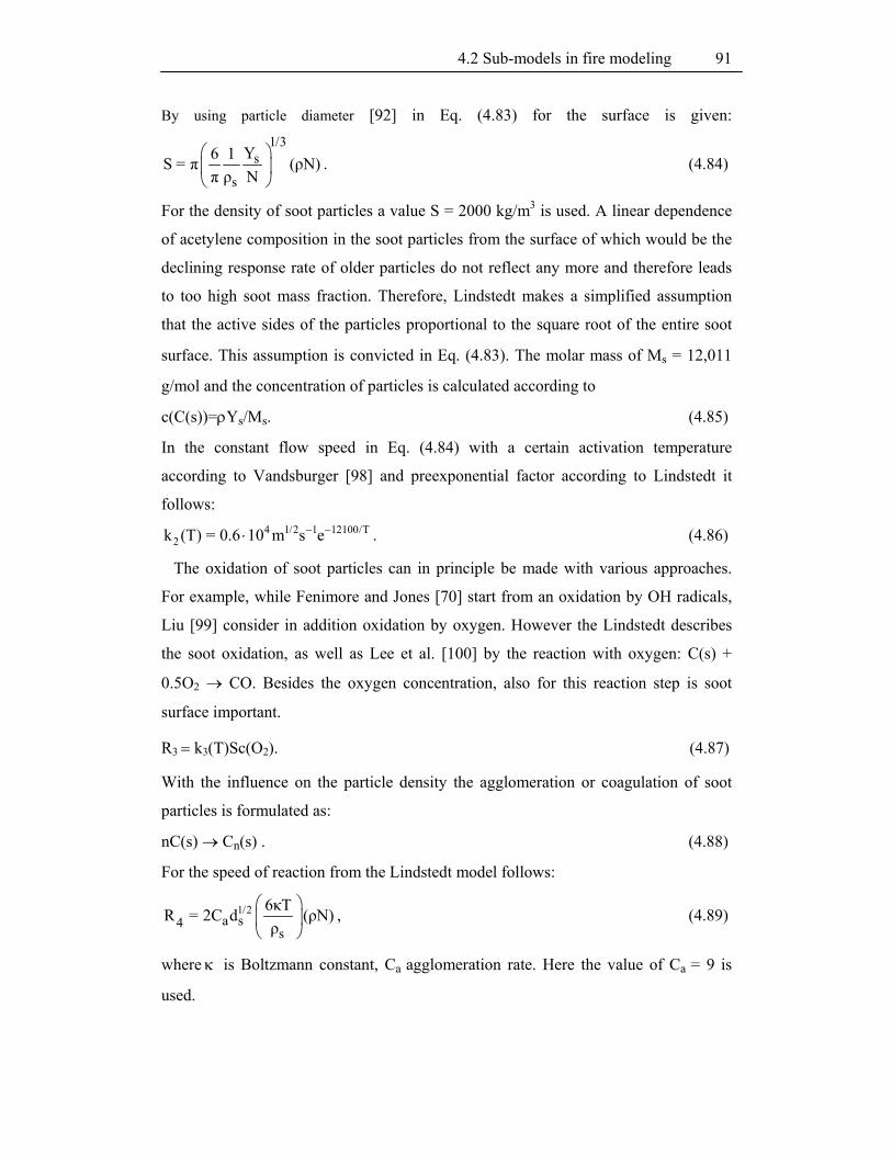
4.2 Sub-models in fire modeling
91
By using particle diameter [92] in Eq. (4.83) for the surface is given:
1/3s
s
Y6 1S = π (ρN)
π ρ N
. (4.84)
For the density of soot particles a value S = 2000 kg/m3 is used. A linear dependence
of acetylene composition in the soot particles from the surface of which would be the
declining response rate of older particles do not reflect any more and therefore leads
to too high soot mass fraction. Therefore, Lindstedt makes a simplified assumption
that the active sides of the particles proportional to the square root of the entire soot
surface. This assumption is convicted in Eq. (4.83). The molar mass of Ms = 12,011
g/mol and the concentration of particles is calculated according to
c(C(s))=Ys/Ms. (4.85)
In the constant flow speed in Eq. (4.84) with a certain activation temperature
according to Vandsburger [98] and preexponential factor according to Lindstedt it
follows:
4 1/2 1 12100/T2k (T) = 0.6 10 m s e . (4.86)
The oxidation of soot particles can in principle be made with various approaches.
For example, while Fenimore and Jones [70] start from an oxidation by OH radicals,
Liu [99] consider in addition oxidation by oxygen. However the Lindstedt describes
the soot oxidation, as well as Lee et al. [100] by the reaction with oxygen: C(s) +
0.5O2 CO. Besides the oxygen concentration, also for this reaction step is soot
surface important.
R3 k3(T)Sc(O2). (4.87)
With the influence on the particle density the agglomeration or coagulation of soot
particles is formulated as:
nC(s) Cn(s) . (4.88)
For the speed of reaction from the Lindstedt model follows:
1/2a s4
s
6κTR = 2C d (ρN)
ρ
, (4.89)
where is Boltzmann constant, Ca agglomeration rate. Here the value of Ca = 9 is
used.

4 Some important topics of CFD used in this work 92
From the above reaction the source for the balance equation of the particle density N
is:
1/6 11/6N A 1 4
min
2S = N R k (T)c(C(s)) (ρN)
C , (4.90)
Where the number of carbon atoms is defined Cmin = 100 (s.o.), NA is the Avogadro
constant. The source for the balance equation for soot mass fraction is calculated
according to the following equation:
P PU v . (4.91)
From the described reaction mechanism follows that by soot oxidation although soot
mass fraction declines, the number of particles or particle density, however, remains
unchanged. Simplification, however, provides a well-to-use mechanism for the
purpose of this work as accurate enough to be considered.
4.2.4.3 Tesner soot model
The two-step Tesner model [84,93] predicts the generation of radical nuclei and then
computes the formation of soot on these nuclei. The combustion of the soot (and
particle nuclei) is assumed to be governed by the Magnussen combustion rate
[83,84,92].
The transport equations are solved for two scalar quantities: the soot mass fraction
(Eq. 4.92) and the normalized radical nuclei concentration:
** * *NN N N
N
tj
t,
μρX+ (ρu X ) = X + R
t Pr
( )
∂ ∇ ∇ ∇∂
(4.92)
where
*NX = normalized radical nuclei concentration (particles · 10–15/kg)
Nt,Pr = turbulent Prandtl number for nuclei transport
*NR = normalized net rate of nuclei generation (particles · 10–15/m3 – s).
In these transport equations, the rates of nuclei and soot generation are the net rates,
involving a balance between formation and combustion.
The two-step model computes the net rate of soot generation, Rsoot, in the same way
as the single-step model, as a balance of soot formation and soot combustion:
Rsoot = Rsoot,form– Rsoot,comb. (4.93)

4.2 Sub-models in fire modeling
93
In the two-step model, however, the rate of soot formation, Rsoot,form depends on the
concentration of radical nuclei, cnuc:
Rsoot,form = ms(– Nsoot)cnuc (4.94)
where
ms = mean mass of soot particle (kg/particle)
Nsoot = concentration of soot particles (particles/m3)
cnuc = radical nuclei concentration = ρbnuc (particles/m3)
a = empirical constant (s–1)
b = empirical constant (m3/particle-s)
The rate of soot combustion, Rsoot,comb is computed in the same way as for the single-
step model, using (Eq. 4.93).
The default constants for the two-step model are for combustion of acetylene (C2H2).
These values should be modified for other fuels, since the sooting characteristics of
acetylene are known to be different from those of saturated hydrocarbon fuels.
The net rate of nuclei generation in the two-step model is given by the balance of the
nuclei formation rate and the nuclei combustion rate:
* * *nuc nuc,form nuc,combR = R R (4.95)
where
*nuc,formR = rate of nuclei formation (particles · 10–15/m3-s)
*nuc,combR = rate of nuclei combustion (particles · 10–15/m3-s)
The rate of nuclei formation, *nuc,formR depends on a spontaneous formation and
branching process, described by
0 0* * *
nuc nuc sootnuc,formR = μ + (f g)c g c N (4.96)
E/RT0 0
* *fuelμ = a c e (4.97)
where
*nucc = normalized nuclei concentration (ρb *
nuc)
0*a = a0/1015
a0 = pre-exponential rate constant (particles/kg–s)

4 Some important topics of CFD used in this work 94
cfuel = fuel concentration (kg/m3)
f – g = linear branching – termination coeffcient (s–1)
g0 = linear termination on soot particles (m3/particle–s)
Note that the branching term, (f – g)c*nuc, in Eq. 4.96 is included only when the
kinetic rate, µ0, is greater than the limiting formation rate (105 particles/m3–s, by
default).
The rate of nuclei combustion is assumed to be proportional to the rate of soot
combustion:
** nucnuc,comb soot,comb
soot
bR = R
Y (4.98)
where the soot combustion rate, Rsoot,comb is given by Eq. 4.93.
Additional inputs include the stoichiometry of the fuel and soot combustion and (for
the two-step model only) the average size (diameter) and density of the soot particles
used to compute the soot particle mass, ms, in Eq. 4.94 for the two step model.
Stoichiometry for soot combustion is the mass stoichiometry, νsoot, which computes
the soot combustion rate in both soot models. The model assumes that the soot is pure
carbon and that the oxidizer is O2. The default value supplied by ANSYS FLUENT
[84] is for combustion of propane (C3H8) by oxygen (O2).
4.3 ANSYS CFX and FLUENT software
4.3.1 Discretisation methods and solution algorithms
4.3.1.1 Finite volume method
The concept of discretization assumes, in the numeric, the transfer of a continuous
function in one function, which only eventually many points are considered. As
discussed in the previous chapters, balance equations can not analytically be solved,
the differential quotient by a difference in discretization quotient must be transferred.
As part of this work a very widespread method of finite volume is applied, i.e. the
balance area is to maximize the number of divided control volumes. This creates a
computational grid with discrete nodes. A part of a two-dimensional mesh or grid is
shown in Fig. 4.8. This is a reassembling grid, which means that not all sizes have the
same grid points. The vector sizes such as the flow speeds are sent to the cell edge
view, the scalar variables such as pressure are saved in the cell centers. Grids are often

4.3 ANSYS CFX and FLUENT software
95
shifted from numerical stability reasons. The differential equations are numerically
considered only to the discrete points. According to the definition of derivation of a
differential function
x 0
xx+Δxdlim
dx x
, (4.99)
the differential operator at the grid point P is approximated by a differential operator
[101]:
E P
P
d
dx x
. (4.100)
In this example a so called right side difference is used, also the left side difference is
possible here [88]
P W
P
d
dx x
, (4.101)
or also a central difference [101]
W
P
d
dx 2 xE
. (4.102)
The central difference is assigned by square order error (1/(x)2), i.e. by half of the
increment will discretisation error for about a factor of four reduced.
Discretisation error by the left-right differences has the magnitude of (1/x), i.e. a
halving of the increment will diskretisation error roughly half. Despite the favorable
error the central difference is not suitable for all problems. For convection-diffusion
problems, in which the convection stream dominates, it is often too unphysical e.g.
oscillations overshoot the numerical solution (Fig. 4.9) when the grid lengths are not
small enough. In such cases often preferred unilateral differences, with the flow
direction must be taken into account. If the flow in the example shown in Fig. 4.8 pass
the grid from west to east as the calculation must be done by the left-hand difference
in a reverse flow direction facing with the right difference. Because of the dependence
of the flow direction Upwind discretisation method is described. The Upwind
discretization of 1st order has the disadvantage that sometimes unrealistic, numerical
diffusion effects are introduced (Fig. 4.9). Nevertheless, they occur by their numerical
stability in many turbulent flows therefore for the solution of the equations of the k-ε
turbulence model is used. There exist Upwind discretizations of higher orders but
these are not available in the CFX or FLUENT solver.

4 Some important topics of CFD used in this work 96
Fig. 4.8: Notation in a staggered two-dimensional numerical grid. The abbreviations
N, E, S and W indicate the relative positions north, east, south and west in relation to
the point P. In addition, the flows n, e, s and w in the neighboring cells are displayed.
In the context of this work is for the discretization in the three directions of all
except the equations of turbulence called high resolution method is used. For the
value of P at the point P is given [83]:
P UPΦ = Φ + β ΦΔv
(4.103)
with the value UP Upwind point and vector v
, the vector directed to point P. The
factor lies in the range from zero to one. For values 0 < < 1 is equal to the
average of neighboring gradients, in the case = 1 is equal to the gradient of Upwind
point. Thus determines whether a method first or second order is applied. In areas
where the size considered only relatively low gradient, is used as close as possible to
1, approximated in areas of high volatility, however, its tends to zero. In this way the
benefits of precision of second order methods will be combined with the numerical
stability of the Upwind method.
4.3.1.2 Geometry and mesh generation
Coupled solver and multi-grid procedure
Application of the finite volume method to all elements in the balance field leads to a
discrete set of linear balance equations in the form
nbi i i
nbi
a = b (4.104)
with the number of i control volumes and the knots point P, the solution , the

4.3 ANSYS CFX and FLUENT software
97
coefficient a of the equation, the right side b and the neighbors nb of i. For a scalar
size are all nbia , nb and bi one number, for the coupled set of balance equations for
mass and momentum both are a matrix or a vector [83]:
nbu u u u u u u px x x y x z x
u u u u u u u py x y y y z ynbi u u u u u u u pz x z y z z z
pu pu pu ppx y z i
a a a a
a a a aa =
a a a a
a a a a
,
x
yi
z
i
u
u
u
p
,
ux
uyi
uz
p i
b
bb =
b
b
. (4.105)
The solver of ANSYS CFX (version 11) uses the coupling of the equations when all
rows are using the same solution methods. The advantage of this method, also in the
non-coupled or iterative solver used by FLUENT (version 12) lies in its stability and
its simplicity [84], and as a disadvantage, higher memory requirements. The overall
solution strategy is illustrated in Fig. 4.9. For each time step occur two compute
intensive operations. First, the non-linear equations must become linear to get the
coefficients for the solution of matrix. Thereafter, the linear equations must be solved
by using an algebraic multigrid method. In the stationary case, the iterations are
controlled by the time step size to target the solution. In transient calculations the time
step size or the maximum number of iterations per time step are performed by the
user. In the presented solution strategy is therefore an iterative method in which the
exact solution by repeated calculations is approximated. CFX 11 is used to solve the
discrete system of linear equations through a multigrid accelerated procedure ILU
(incomplete lower upper) solver. The linear system of discrete equations is taking into
account the coefficient matrix [A] and the solution vector [] to be formulated as
follows [83]:
[A][]=[b]. (4.106)
With an iterative method is an approximate solution considered to be improved by a
correction factor [83]:
nn+1 . (4.107)
A corrector value is solution of the equation [83]
nA = r , (4.108a)
and rn is residual from n nr = b A . (4.108b)
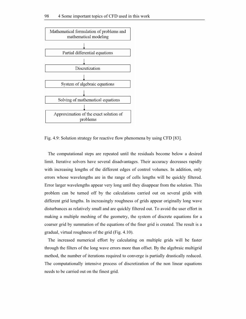
4 Some important topics of CFD used in this work 98
Fig. 4.9: Solution strategy for reactive flow phenomena by using CFD [83].
The computational steps are repeated until the residuals become below a desired
limit. Iterative solvers have several disadvantages. Their accuracy decreases rapidly
with increasing lengths of the different edges of control volumes. In addition, only
errors whose wavelengths are in the range of cells lengths will be quickly filtered.
Error larger wavelengths appear very long until they disappear from the solution. This
problem can be turned off by the calculations carried out on several grids with
different grid lengths. In increasingly roughness of grids appear originally long wave
disturbances as relatively small and are quickly filtered out. To avoid the user effort in
making a multiple meshing of the geometry, the system of discrete equations for a
coarser grid by summation of the equations of the finer grid is created. The result is a
gradual, virtual roughness of the grid (Fig. 4.10).
The increased numerical effort by calculating on multiple grids will be faster
through the filters of the long wave errors more than offset. By the algebraic multigrid
method, the number of iterations required to converge is partially drastically reduced.
The computationally intensive process of discretization of the non linear equations
needs to be carried out on the finest grid.

4.3 ANSYS CFX and FLUENT software
99
Fig. 4.10: Multigrid procedure: generation of larger grid strikes so as virtual
amalgamation of individual cell [83].
4.4 Procedure of CFD simulations
In this work, JP-4 pool fire is simulated as a prototype of sooty hydrocarbon fires. The
CFD simulation is done by using different sub-models contained in softwares ANSYS
CFX and FLUENT. The different pool diameters are used to show that the
experimentally found dependence of various parameters such as temperature and
thermal radiation on pool diameter in the calculations realistically reproduced the
experimental data. An overview of the simulations and the set of sub-models can be
found in Tab. 4.1.
The indication of modeling consists of the initial letters of fuel and the pool
diameter in meters. The remarks on the geometry and grid generation, selection and
configuration of the sub-models and the definition of initial and boundary conditions
will be made in subsequent chapters.
The main purpose of CFD simulation was to determine the temperature T, Surface
Emissive Power (SEP) and irradiance E. The simulations are started by using k-
turbulence model with a buoyancy correction term [83] to reach a certain height of the
flame which refer to the developing stage of the fire (approx. t = 10 s). After a
simulation time of t = 10 s it is assumed that the flame is developed and the further

4 Some important topics of CFD used in this work 100
simulation is continued by using Scale Adaptive Simulation (SAS) [83] or Large
Eddy Simulation (LES) [84].
Table 4.1. Overview of the modeling
Geometry 3D cylindrical 3D cylindrical 3D cylindrical 3D cylindrical
Pool diameter 2 m 8 m 16 m 25 m
Turbulence model k-, SAS, LES k-, SAS k-, SAS, LES k-, SAS
Combustion model Flamelet Flamelet Flamelet Flamelet
PDF transport Multistep PDF transport
Soot model Lindstedt Lindstedt Lindstedt Lindstedt
Tesner Magnussen Tesner
Radiation model Monte Carlo Monte Carlo Monte Carlo Monte Carlo
Discrete Ordinate Discrete Ordinate
Time interval 0 ≤ t ≤ 10 s 0 ≤ t ≤ 10 s 0 ≤ t ≤ 10 s 0 ≤ t ≤ 10 s
11 s ≤ t ≤ 20 s 11 s ≤ t ≤ 20 s 11 s ≤ t ≤ 30 s 11 s ≤ t ≤ 20 s
4.4.1 Geometry and meshing
4.4.1.1 Geometry and meshing for the fire in calm condition
In the CFD simulation of large JP-4 pool fires a domain is presented as a 3D
cylindrical hexahedral non uniform unstructured mesh (Fig. 4.11). The mesh is very
refined at the pool surface and in the inner part of domain with increasing cell
dimension as moving to the side boundaries. Dimensions of the geometry and mesh
refinement for each pool diameter are listed in the Tab. 4.2.
The fire domain initially contains air under ambient conditions: Ta = 293 K and pa
= 1.013 bar.
The definition of simplified geometry leads to a significant reduction of the time.
The geometries are described in detail.

4.4 Procedure of CFD simulations
101
Fig. 4.11: Example of 3D hexahedral unstructured mesh used in simulation of JP-4
pool fires (d = 2 m, 8 m, 16 m and 25 m).
Table 4.2: Dimensions of the geometry and mesh refinement for different d
d (m) 2 8 16 20 25
Dimensions (m2)
r x 3 6 10 40 20 60 30 60 30 60
Number of cells (106) 0.35, 0.8 0.4, 1 1 0.4, 1 1
Cell length (m)
Min 0.05, 0.01 0.1 0.3 0.30 0.30
Max 0.1, 0.08 0.2 0.3 0.55 0.55
Rim height (m) 0.05 0.1 0.5 0.5 0.5
4.4.1.2 Geometry and meshing for the fire under the wind influence
In a case of CFD simulation of large JP-4 pool fires under the influence of cross-wind
coarser meshes are used than in a case of the CFD simulation of a fire. The
rectangular geometry is chosen to predict the flame tilt under the wind influence. An
example of the geometry is shown on the Fig. 4.12. Dimensions of the geometry and
mesh refinement for each pool diameter are listed in the Tab. 4.3.

4 Some important topics of CFD used in this work 102
Fig. 4.12: Example of 3D hexahedral unstructured mesh used in simulation JP-4 pool
fire (d = 2 m, 20 m and 25 m) under the wind influence.
Table 4.3: Dimensions of the geometry and mesh refinement for different d
d (m) 2 20 25
Dimensions (m2)
x y 6 4 60 40 60 40
Number of cells (106) 0.3 0.3 0.3
Cell length (m)
Min 0.05 0.3 0.3
Max 0.1, 0.08 0.5 0.5
Rim height (m) 0.05 0.1 0.5
4.4.2 Initial and boundary conditions and time steps
The boundaries and the initial conditions are partially identical for two geometries
with the difference that an additional inlet boundary surface is used in the case of the
geometry used for the simulation of the fire under the wind influence. At that inlet

4.4 Procedure of CFD simulations
103
boundary an air flow with a certain velocity which refers to the wind speed is assigned
(Fig. 4.12). As the fluid in domain an air is assumed to consist of nitrogen, oxygen
and carbon dioxide. The existence of the species carbon dioxide and water at the
beginning of the reaction when eddy dissipation model is used is essential. The model
does not take into account kinetic time scales but the concentrations of various species
and the turbulence in the form of k and ε. The mass fractions of individual species in
temperature in domain is Tamb = 293 K and the pressure is defined relative to the
reference pressure pamb = 1.013 bar.
As the mass burning rate experimentally determined value for JP-4 and [25] is used.
At the time t = 0 s, the flame is ignited in the experiment, or begins in the
computational modeling. From that time initially grows in the size until some time
after its full size is reached. In the first test calculations have shown that the flames
with a pool diameter 2 m ≤ d ≤ 25 m at the minimum time of t = 10 s reach their full
size, the smaller pool of flame with d = 2 m already after about t = 5 s.
It appears in the experiments [102,103] that analogous to the growth of the flame,
the mass burning rate from a minimum based on a nearly constant value increase. In
simulations the constant mass burning rate is used.
For the JP-4 pool fires simulations time steps in a range of 0.0001 s ≤ ∆t ≤ 0.01 s are
chosen to reach achieved convergence level of minimum 10–3 independently on d but
depending on the sub-models. Number of iterations per time step varied from 3 to 15
depending on chosen sub-models, where at the beginning of simulation a large
number of 10 – 15 iterations per time step is used and after the convergence is reached
the number of iterations decreased to minimum 3 – 5. For example in a case of
simulations where LES and flamelet model are used, simulation started with the
largest time step of 0.01 s and 15 iterations per time step and finally after the achieved
convergence is reached a time step of 0.001 s – 0.0025 s is used with 5 iterations per
time step, whereas in a case of simulations where SAS and flamelet model are used,
simulation started with the smallest time step of 0.0001 s and 10 iterations per time
step and when the achieved convergence is reached a time step is increased to the
maximal 0.005 s – 0.01 s with 3 – 5 iterations per time step used.
The fuel is assumed to be already evaporated and the fuel vapor coming from the
inlet boundary surface with defined constant temperature Tin = 373 K and a constant

4 Some important topics of CFD used in this work 104
mass flow rate of fuel, fm . fm are based on experimentally determined mass burning
rates fm [25]. In Tab. 4.4 fm and fm
for different d are listed.
The inlet is surrounded with a low rim (Tab. 4.2, 4.3) and adiabatic ground area.
The remaining areas in the computational domain are open boundaries with defined
ambient conditions. In CFD simulation a non uniform mesh (Tab. 4.2, 4.3) is used
with the minimum cell length at the inlet surface and in the near surrounding. With
increasing a vertical distance from the pool the cell size increases and reaches the
maximum length. The time steps vary depend on the sufficient convergence from t =
10–5 s to t = 10–2 s. The number of iterations per time step is 5 – 10.
Table 4.4: fm and fm of JP-4 pool fire for different d.
d (m) 2 8 16 20 25
fm (kg/(m2 s)) 0.054 0.054 0.054 0.054 0.054
fm (kg/s) 0.17 2.7 10.8 17.0 26.5
JP-4 pool fires (d = 2 m, 20 m and 25 m) were simulated under the influence of cross
wind with various wind speed used as corresponding to test data from JP-4 pool fires
(d = 2 m, 2.5 m, 3 m, 18.9 m, 20 m and 25 m) [3,9-11,16,18,19]. Wind is defined as
an airflow directed to the one of the side boundaries in the rectangular geometry
assumed to have a constant velocity at the whole boundary surface. 3D transient
simulations are started with zero wind until simulation time of t = 5 s after which a
certain wind velocity is applied. After t = 10 s when the relatively steady flame shape
is achieved it is assumed that the wind had a certain effect on the flame so that
averaging of data is done for a time interval of 10 s ≤ tb ≤ 20 s. The k-ε turbulence
model with buoyancy correction term is used until the t = 10 s of the simulation time
after which the LES (JP-4, d = 2 m) or SAS (JP-4, d = 20 m and 25 m) is used until t
= 20 s. Time steps used were in a range of ∆t = 0.00025 – 0.01 s for 0.35 · 106 mesh
(d = 2 m) and ∆t = 0.005 – 0.02 s for 0.3 · 106 mesh (d = 20 m and 25 m) which
minimum is 2.5 times larger than the ∆t used in a case of calm conditions for the same
mesh refinement.
4.4 Procedure of CFD simulations
105
4.4.3 Determination and configuration of sub-models
The following sub-models are used:
- k- ε turbulence model
- Scale Adaptive Simulation (SAS)
- Large Eddy Simulation (LES) Smagorinsky
- Laminar flamelet model with PDF for non premixed combustion containing
112 species and 800 chemical reaction,
- PDF transport model containing 20 species and 60 chemical reaction,
- Multistep chemical reaction containing 6 species and 6 chemical reaction,
- Monte Carlo radiation model,
- Discrete Ordinate radiation model
- Linstedt soot model,
- Tesner soot model.
4.4.3.1 Sub-models for turbulence
4.4.3.1.1 k-ε model
In Section 4.2.1. several turbulence models have already been discussed. The most
commonly used two-equation models such as the k-ε model have not initially been
developed for certain buoyancy, anisotropic, turbulent natural convection flows.
Large eddy simulation appear in the description of such flows very capable, but its
demands a large computational effort since the vortex are then calculated directly,
without any model assumptions, the model demands a very fine discretization in space
and time. This means a fine meshing of geometry, in particular, but also a choice of a
very small time step of t = 10–4 s is necessary. As the flames in the context of this
work are simulated over a period of about ttot = 20 s – 30 s, a too high computational
effort was in demand when LES and SAS models are used with flamelet models. With
the expected increase in computing power of modern computers and the possibility of
parallel calculations on inexpensive PC clusters to implement, a standard use of large
eddy simulations for pool flames in the near future can be expected. The k-ε model
with buoyancy terms needed, in comparison to LES, a much larger time steps of 0.01
s ≤ ∆t ≤ 0.05 s, a significantly less computationally intensive, and also can give fairly
good results with in modeling similar flows [17-19].

4 Some important topics of CFD used in this work 106
In this work the CFD simulation is started at t0 = 0 with a k- turbulence model with
a buoyancy correction term [83,84] to reach a certain height of the flame. At t = 10 s
the flame is developed and for t > 10 s during a burning time of tb = 10 s a further
simulation of a flame is performed by using Large Eddy Simulation (LES) or Scale
Adaptive Simulation (SAS). The burning time tb starts at 10 s when the flame is
developed and ends at 20 s limited by the CPU time. This means that the flame during
the burning time of 10 s show a real burning.
4.4.3.1.2 Large Eddy Simulations (LES) Smagorinsky
Here, dynamic LES Smagorinsky model is used in simulation with FLUENT
software.
The Large Eddy Simulation (LES) is a method for numerical calculation of
turbulent flows with high Reynolds numbers. These are the Navier-Stokes equations
locally and coincided with a low pass filter filtered. Thus, the large vortex structures
are directly calculated and the small structures are modeled with one of the RANS
turbulence models [104]. The computing lies between direct numerical simulation
(DNS) and the solution of Reynolds equations, RANS (Reynolds averaged Navier
Stokes) which only calculates an averaged value, so the computation time is
significantly lower than in the DNS.
4.4.3.1.3 Scale Adaptive Simulations
In this work SAS is used in simulation with CFX software.
Scale Adaptive Simulation (SAS) models are advanced URANS (Unsteady RANS)
models which allows a realistic calculation of unsteady flows. Unlike standard
URANS methods that typically resolve only large scale structures SAS allows a
decline of greater turbulence elements in a turbulent spectrum. SAS achieved the
improvement in the transient field by taking into account the Karman length scale in
the scaling of the equation turbulence model. This allows the model already resolved
structures and avoids the smearing which is in the standard URANS methods typical.
A detailed mathematical description can be found in CFX guideline [83].

4.4 Procedure of CFD simulations
107
4.4.3.2 Sub-models for combustion
For the modeling of the JP-4 pool fires, the Eddy dissipation model and the different
flamelet models are chosen. The choice of combustion model is done depending on
simulation type. For the simulation of fires in a calm condition, mostly a laminar
flamelet model has been used. Some simulations are done by using different
combustion models e.g. flamelet model and Eddy dissipation model e.g. JP-4 pool fire
with d = 8 m and d = 25 m to investigate the influence of combustion models on
predicted temperature and SEP of the fire. The simulations with the fires under the
wind influence are done in some cases (JP-4 pool fire with d = 20 m and 25 m) by
using Eddy dissipation model with multistep chemical reaction (6 reactions and 6
species).
The choice of the combustion model, depending on the grid refinement and
environment fire condition simulated.
4.4.3.3 Sub-models for thermal radiation
While the heat conduction in solids is the only type of heat transport, in turbulent
flows plays a minor role. Here dominate depending on the temperature, either the
convection or thermal radiation. The different modeling of the thermal radiation in the
simulation program ANSYS CFX and FLUENT can be found in [83,84].
The balance equation for the thermal radiation is given as
L
λabs,λ scat,λ λ abs,λ λ
scat,λ λ
dL (r, s)= (k + k )L (r, s) k L (r, s, T) +
dl(a) (b)
k dL (r, s) (s, s , )d + S
(c) (d)
(4.109)
Term (a) with the absorption kabs and scattering coefficients and kscat refer to
increasing the radiation intensity in the direction r,s; term (b) refer to the black body
radiation with kabs; term (c) refer to the re-emitted radiation from all other directions
with kscat and term (d) refer to the additional heat source SLλ.
In the following text the different radiation models used in this work are discussed.

4 Some important topics of CFD used in this work 108
4.4.3.3.1 Discrete Ordinate radiation model
In addition to Monte Carlo simulations are also the discrete transfer radiation method
in the modeling in pool flames enforced. Here, the radiance L is not through the
pursuit of a very high number of photons identified, but along the less number of rays
calculated. This way, the computing time compared to the Monte Carlo method
significantly shortened. These simplifications, however, are necessary, which may
distort the result. The discrete ordinate method [84] assumes an isotropic scattering
from. Eq. (4.109) thus simplifies to
λ L4
abs,λ scat,λ abs,λλ λ
scat,λ
dL (r, s)λ= (k + k )L (r, s) + k L (r, s )
dl
k + (r, s )d + S
4π
, T
dL
(4.110)
Furthermore it is assumed that the balance area has relatively homogeneous radiation
characteristics, such that [83]:
λ λL (r) L (r + dr) (4.111)
The intensity is then along rays, with L, 0 from the edges of the balance area, using
the following equation [95]:
λS,λλ λ,0 abs,λ scat,λ abs,λ scat,λL (r,s) = L exp( (k + k )l) + L (1 exp( k l)) + k L )
. (4.112)
Usually, 8 – 16 rays in the balance area are prosecuted. The extension of the results
along the ray paths to the entire record area is under the above assumption of
homogeneity of the area. In the case of a gray medium, the intensities are only
calculated once per ray. If, however, for example, different bands of a gas have to be
taken into account, the first solution for each corresponding wavelength can be
calculated. Finally, the integration over the individual results is done to determine the
overall intensity.
4.4.3.3.2 Monte Carlo radiation model
Monte Carlo simulations are applicable for many different problems, such as in
meteorology to forecast climate change, or even in the financial industry for the
prediction of exchange rates. The Monte Carlo method is one of the most robust
numerical methods to calculate the heat transfer by radiation. Its advantage lies in the

4.4 Procedure of CFD simulations
109
possibility to simulate the radiation heat transfer in arbitrary geometric configurations,
taking into account the spatially varying optical properties of a medium radiation in a
simple way. When used the Monte Carlo method is a representative number of
photons in the entire simulation area emitted. The starting points and the beginning of
the individual photons are randomly chosen. Therefore, it must be ensured that a
sufficiently large number of photons is created to ensure a realistic picture of
radiation. The probability that a photon in a particular place, or in a given cell along
the beam path is scattered or absorbed, is determined by the spatially variable
absorption kabs or kscat scattering coefficients. In the following chapters kabs will be
replaced with a modified absorption coefficient æ . The irradiance E in a given area is
equal to the number of counted on it taken photons multiplied by the associated
emissivity [83]. The crucial disadvantage of the Monte Carlo method is that it is very
computationally intensive, if a good accuracy of results is desired. This is particularly
true when the Monte Carlo method as in the context of this work with other methods
such as finite differences or finite volume method is coupled. Due to the large number
of cells, the number of required computational steps is accordingly high. Also, the
stability of time integration schemes in the case of transient problems is heavily
influenced by the accuracy of the results of a Monte Carlo simulation. The spatially
and temporally varying temperatures and species concentrations in flames cause the
equally variable emission or absorption.
4.4.3.4 Sub-models for soot
4.3.3.1 Magnussen soot model
The soot modeling according to Magnussen [92] represents a direct extension of the
Eddy dissipation model for the calculation of combustion products such as soot and
NOx. For calculation of the soot in the Magnussen model several steps are used:
Source terms of species
1. Soot formation in the of form radicals,
2. Formation of soot particles from the radicals,
3. Oxidation of soot particles and radicals,
4. Calculation of the influence of turbulence on the reaction rates with Magnussen
and Eddy dissipation model.
4 Some important topics of CFD used in this work 110
The two sizes will be required: for the soot mass fraction Ys and the specific
concentration of radicals XN. The two balance equations contain a term for formation
and oxidation the respective sizes. More detail description of the model can be found
in Section 4.2.4.1.
Table 4.5: Standard values of parameters in Magnussen model [83]
Parameter Value Value (mol)
sρ 2000 [kg/m3]
ds 1.75 · 10-8 [m]
a0 1.35 · 1037 [1/(kg s)] 2.24 · 1013 [mol/(kg s)]
fC carbon mass fraction in fuel (e.g. 12/16 for methane)
TA,0 90000 [K]
f-g 100 [1/s]
g0 1.0 · 10-15 [m3/ s] 6.02 · 108 [m3/(s mol)]
a 1.0 · 105 [1/s]
b 8.0 · 10-14 [m3/ s] 4.98 · 1010 [m3/(s mol)]
4.3.3.2 Soot modeling with Lindstedt
Lindstedt model leads to soot modeling two sizes, for one so-called particle density N,
the number of particles per mass of mixture states, and continue to soot mass fraction
Ys [83,105]. The determination of the source terms SN and YsS is described in
Section 4.2.4.2. Experiments show that acetylene plays an important role in the
different processes of soot occupies (Chap. 2.5.3). For the first acetylene molecule
PAHs can be built later in the HACA mechanism which can be involved in sub-
models. Accordingly, Lindstedt describes the nucleation and the growth of surface as
a function of acetylene concentration. Details in modeling of soot formation can be
found in [91,105].
4.3.3.3 Tesner soot model
The formation of radicals and soot are modeled according to Tesner et al. [93]. The
formation of soot and nuclei particles is given as [84,93]:

4.4 Procedure of CFD simulations
111
The equations included in the model depend on the formation and oxidation of soot
particles and the radicals from the fuel mass fraction from. This fact represents a large
numerical advantage, for the source of the JP-4 as a fuel calculated with the Eddy
dissipation model and represents the influence of turbulence on combustion. As the
source of the solution according to the fuel balance equation exists, no additional
computing time steps for the consideration of turbulence on soot are required. This
direct dependence can also prove detrimental. Since the fuel mass fraction is
calculated here in the large pool fire in a relatively low dimensionless heights x/d
mainly with increasing distance from the flame axis reach very small values, the
oxidation terms for the soot particles and the radicals in many areas of the flame is
also very small. Considering the relatively complicated soot formation mechanism
consists of on the various intermediate steps such as nucleation, formation of the
primary particles, particle growth and oxidation, in the soot oxidation model a
significant simplification is used in CFD models. More details about the model can be
found in Section 4.2.4.3.
4.4.4 Modeling of absorption coefficient of the flame
Absorption coefficients used in the radiation model OSRAMO II, III [7,27] contained
in effective absorption coefficient of the flame effæ (T)ˆ assume influence of air
absorption airæ (T)ˆ = 0.02 m1, absorption of soot parcels spæ (T)ˆ = 1.035 m1, hot
spots hsæ (T)ˆ = 0.404 m1 and reactive zone reæ (T)ˆ = 0.380 m1. Sinai et al [17] use
step function of averaged absorption coefficient æ which contains absorption
coefficient of air airæ = 0.02 m1 and æ of fuel/air reacting mixture f +airæ = 0.5 m1
which decrease the influence of soot absorption. Mc Grattan [15] use constant æ =
0.05 m1 of a flame (gaseous combustion mixture of fuel and air) included in SFM,
neglecting a smoke blockage effect which lead to a noticeable increase of calculated
surface emissive power. In [25] a constant absorption coefficient æ = 0.5 m1 is given
for JP-5 gaseous fuel and æ = 2.6 m1 for liquid kerosene fuel.
Tien et. al obtain the following expression for the soot absorption-emission coefficient
by integration of the soot emission over all wavelengths:
æ = 3.6 BRfVT/C2 = CK,RfVT (4.13)
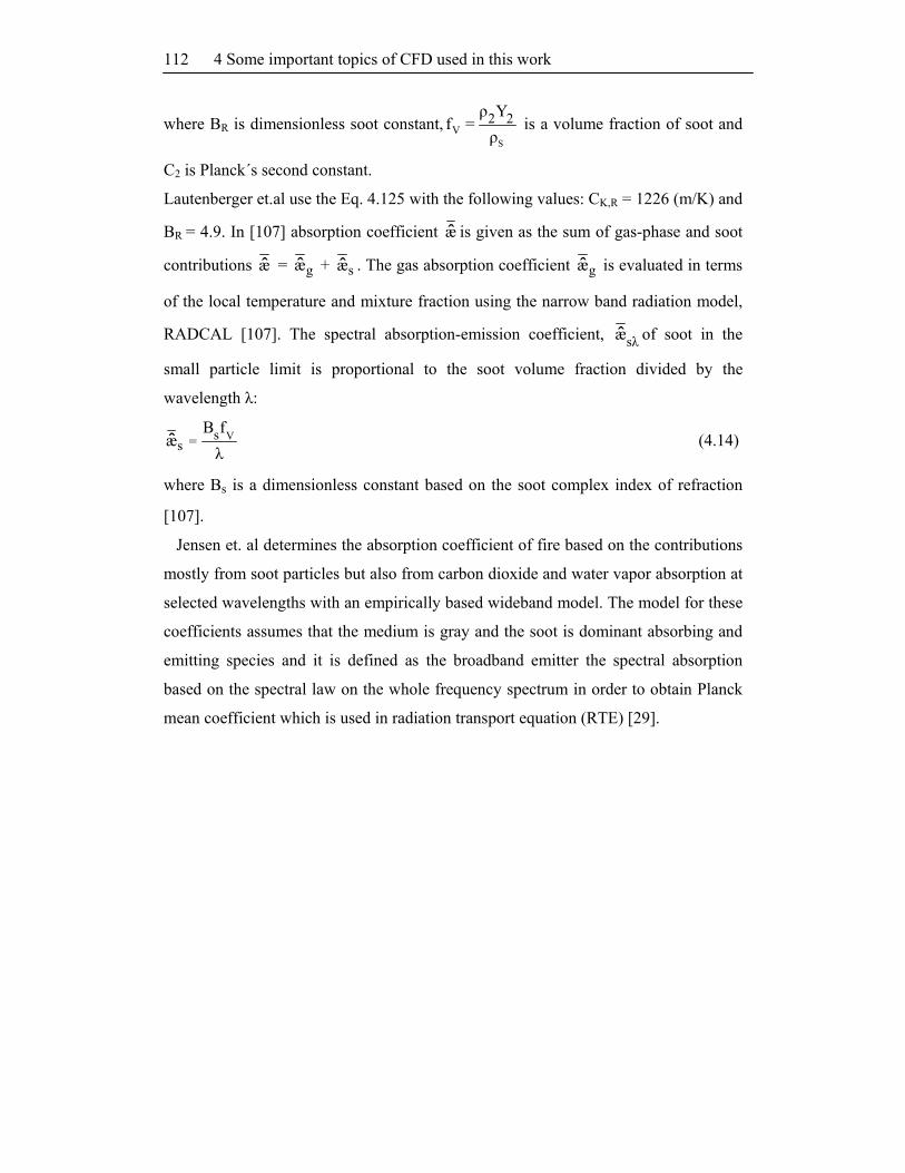
4 Some important topics of CFD used in this work 112
where BR is dimensionless soot constant,S
V2 2ρ Y
f = ρ
is a volume fraction of soot and
C2 is Planck´s second constant.
Lautenberger et.al use the Eq. 4.125 with the following values: CK,R = 1226 (m/K) and
BR = 4.9. In [107] absorption coefficient æ is given as the sum of gas-phase and soot
contributions æ = gæ + sæ . The gas absorption coefficient gæ is evaluated in terms
of the local temperature and mixture fraction using the narrow band radiation model,
RADCAL [107]. The spectral absorption-emission coefficient, sλæ of soot in the
small particle limit is proportional to the soot volume fraction divided by the
wavelength λ:
Vs=sB f
æλ
ˆ (4.14)
where Bs is a dimensionless constant based on the soot complex index of refraction
[107].
Jensen et. al determines the absorption coefficient of fire based on the contributions
mostly from soot particles but also from carbon dioxide and water vapor absorption at
selected wavelengths with an empirically based wideband model. The model for these
coefficients assumes that the medium is gray and the soot is dominant absorbing and
emitting species and it is defined as the broadband emitter the spectral absorption
based on the spectral law on the whole frequency spectrum in order to obtain Planck
mean coefficient which is used in radiation transport equation (RTE) [29].

5. Results and discussions
5.1 Instantaneous and time averaged flame temperatures
5.1.1 Thermograms
The local distribution of temperatures at the flame surface, defined as emission
temperatures T(x, y) is obtained experimentally directly from a thermogram (Figs.
5.1a1 and 5.2) which received thermal radiation from the fire [3,4]. For the emissivity
of large, sooty fire εF = 0.92 is used [2,3]. The IR images obtained from the
thermographic camera were transferred as matrices of temperature using the software
provided with the thermographic camera [3,4]. Each instantaneous thermogram,
consists of the pixel elements of a matrix with 480 rows and 640 columns where Ti,j is
emission temperature of a pixel element at the position (i, j) in a x,y plane of the
thermogram [3,4,27]. The instantaneous thermogram consists of colored areas which
correspond to a defined temperature range ∆T or to a defined range of surface
emissive power ∆SEP [3,4,27]. A series of thermograms of a JP-4 pool fire (d = 16 m)
are presented in Fig. 5.1a1 and four instantaneous thermograms of a JP-4 pool fire (d
= 25 m) are shown in Fig. 5.2.
The instantaneous thermograms of a JP-4 fires (Fig. 5.1a1 and 5.2) show a local
inhomogeneities of temperature and time dependent fluctuations in these flames. The
time averaged emission temperatures i, j
T of pixel elements are obtained from a
series of thermograms by using the instantaneous temperatures Ti,j [3,27]:
NT
T
i, j
i, j
TT
N1
= (5.1)
By CFD simulations the emission temperatures are calculated from SEP by using
Stephan Boltzman law and the SEP is obtained by integration of incident radiation G
along the path length. Detailed procedure is given in Chapter 5.2.6.
The procedure is done as follows:
- The flame is divided into large number (e.g. 50) of parallel planes perpendicular to
the pool surface,
- On the each plane a distribution of incident radiation G(x, y) is plotted,
- The certain path length s between d/4 ≤ s ≤ d/2 through the parallel planes starting
from the flame centerline is chosen for integration of G,

5. Results and discussions
114

5.1 Instantaneous and time averaged flame temperatures
115
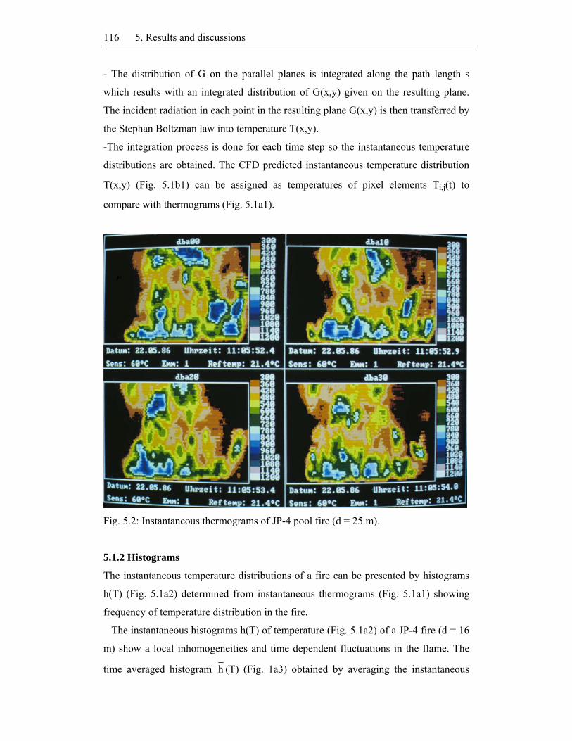
5. Results and discussions
116
- The distribution of G on the parallel planes is integrated along the path length s
which results with an integrated distribution of G(x,y) given on the resulting plane.
The incident radiation in each point in the resulting plane G(x,y) is then transferred by
the Stephan Boltzman law into temperature T(x,y).
-The integration process is done for each time step so the instantaneous temperature
distributions are obtained. The CFD predicted instantaneous temperature distribution
T(x,y) (Fig. 5.1b1) can be assigned as temperatures of pixel elements Ti,j(t) to
compare with thermograms (Fig. 5.1a1).
Fig. 5.2: Instantaneous thermograms of JP-4 pool fire (d = 25 m).
5.1.2 Histograms
The instantaneous temperature distributions of a fire can be presented by histograms
h(T) (Fig. 5.1a2) determined from instantaneous thermograms (Fig. 5.1a1) showing
frequency of temperature distribution in the fire.
The instantaneous histograms h(T) of temperature (Fig. 5.1a2) of a JP-4 fire (d = 16
m) show a local inhomogeneities and time dependent fluctuations in the flame. The
time averaged histogram h (T) (Fig. 1a3) obtained by averaging the instantaneous

5.1 Instantaneous and time averaged flame temperatures
117
histograms with the number NT (e.g. 50) shows a large frequency of emission
temperatures in interval of 793 K ≤ expT ≤ 1033 K [3,4]. Low emission temperatures
are typical for large sooty hydrocarbon pool fires where smoke blockage effect plays a
great role in decreasing of thermal radiation to the surrounding and hence reduction of
emission temperatures. In JP-4 pool fire a relatively large amount of soot is produced
which leads to an increase of thermal radiation of a flame and therefore to an increase
of the flame temperature [27]. However, this increase of the emission temperature is
partially compensated by the smoke blockage effect occurring in the most of
hydrocarbon pool fires, which leads to a certain decrease of thermal radiation and
therefore to a decrease of the emission temperature [27].
The CFD predicted instantaneous histograms hCFD(T) (Fig. 5.1b2) obtained from
thermograms (Fig. 5.1b1) are averaged over a real burning time tb = 10 s to get time
averaged histogram CFDh (T) as shown in the Fig. 5.1b3. The histogram shows a large
frequency of emission temperatures in interval of 700 K ≤ CFDT ≤ 904 K. A
discrepancy between CFD predicted results and the measured data are due to the path
length s chosen for the integration of G. The path length s in ideal conditions should
mimic real path length of the JP-4 pool fire (d = 16 m) what is not easy to determine
in time dependent CFD predicted results, neither in experiments.
5.1.3 Probability density function (pdf)
The time averaged pdf of temperature is determined based on the time averaged
histogram (Fig. 5.1a3). The time averaged temperature at the maximum of the pdf
predicted by CFD, CFDT = 911 K (Fig. 1b3) is for about 38 K higher than the time
averaged measured temperature T = 873 K at the maximum of pdf (Fig. 5.1a3) [3,4].
It must be noticed that the thermograms used here for comparison of CFD results
belongs to one of the series of thermograms of JP-4 pool fire (d = 16 m) given in [3,4]
and the time averaged temperature from thermograms vary from test to test. The
temperatures *T obtained by Gaussian distribution from the measured T (Table 5.1)
[3,4] can be used for comparison with CFD
T . It can be seen that the CFD
T = 911 K is
only slightly larger than the averaged temperature from series of experiments expT =
902 K [3,4].

5. Results and discussions
118
Table 5.1: Averaged values and standard deviation for different thermographic series
for JP-4 pool fire (d = 16 m)
Serie ( *x = x )1 s *T (K) expT (K) CFD
T (K)
A – 0.1651 0.175 848
B – 0.1001 0.200 905
C – 0.0896 0.188 914
D – 0.1290 0.168 879
902
911
1 based on Gauss normal distribution
Table 5.2: Averaged values and standard deviation for different thermographic series
for JP-4 pool fire with different d
d(m) ( *x = x )1 s expT (K)
CFDT (K)
8 – 0.043 0.190 975 980
16 – 0.1205 0.184 902 911
25 – 0.1169 0.187 859 900 1based on Gauss normal distribution
X
X=
*
x1
G (x)dx =2
(5.2a)
where
*x is a mean value
*T = T0 · ex* = T0 · e
x (5.2b)
x = ln(T/ T0) with T0 = 1000 K (5.2c)
Due to the limited number of series of instantaneous thermograms in a visual form,
only one serie of NT = 50 pictures is used for visual comparison with the CFD results.
Also, it should be noted that the slight wind with velocity of changeable strength and
direction was present during the experiments [3,4] which could have an influence on
the heat flux received by thermograms and a temperature distribution, hence the
discrepancy between the measured and CFD results, here in expT and CFD
T . Another
reason is due to the path length s used for integration of G by CFD (Chapter 5.2.6).

5.1 Instantaneous and time averaged flame temperatures
119
Detailed calculation can be found in [3]. Validation of CFD simulation by using
global metric [107] is given in Chapter 5.5.
5.1.4 Temperature fields
A quantitative description of the dynamics of JP-4 pool fires (d = 2 m, 8 m, 16 m and
25 m) is shown in Fig. 5.3.1a,b-5.3.4a,b by the predicted isotherms at three different
times. The first instantaneous temperature field applies to the time t1 = 12 s after
ignition, t2 = 14 s and t3 = 16 s. In the three fields the flame pulsation is noticeable.
The flame pulsation is connected with a formation and rising of vortices which greatly
effect the distribution of the maximum flame temperature. A significant expansion of
small vortices at of the pool rim is visible in all predicted temperature fields. Here,
inside the vortices the temperatures are significantly higher than in a surrounding area,
for 1200 K ≤ T ≤ 1800 K.
t = 12 s
Fig. 5.3.1a: Isotherms of JP-4 pool fire (d = 2 m) at t = 12 s predicted by using
flamelet model.

5. Results and discussions
120
t = 14 s
t = 16 s
Fig. 5.3.1b: Isotherms of JP-4 pool fire (d = 2 m) at t = 14 s and 16 s predicted by
using flamelet model.

5.1 Instantaneous and time averaged flame temperatures
121
t = 12 s
t = 14 s
Fig. 5.3.2a: Isotherms of JP-4 pool fire (d = 8 m) at t = 12 s and 14 s predicted by
using flamelet model.

5. Results and discussions
122
t = 16 s
Fig. 5.3.2b: Isotherms of JP-4 pool fire (d = 8 m) at t = 16 s predicted by using
flamelet model.
t = 12 s
Fig. 5.3.3a: Isotherms of JP-4 pool fire (d = 16 m) at t = 12 s predicted by using
flamelet model.

5.1 Instantaneous and time averaged flame temperatures
123
t = 14 s
t = 16 s
Fig. 5.3.3b: Isotherms of JP-4 pool fire (d = 16 m) at t = 14 s and 16 s predicted by
using flamelet model.

5. Results and discussions
124
t = 12 s
t = 14 s
Fig. 5.3.4a: Isotherms of JP-4 pool fire (d = 25 m) at t = 12 s and 14 s predicted by
using flamelet model.
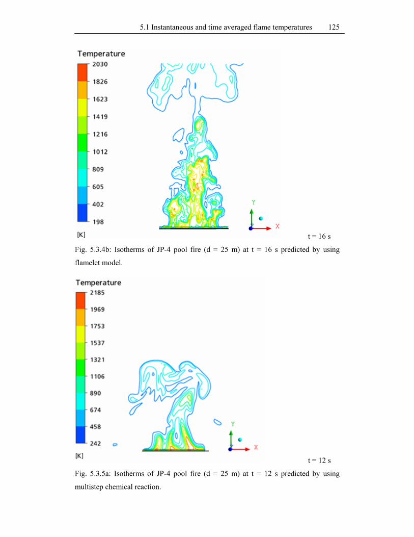
5.1 Instantaneous and time averaged flame temperatures
125
t = 16 s
Fig. 5.3.4b: Isotherms of JP-4 pool fire (d = 25 m) at t = 16 s predicted by using
flamelet model.
t = 12 s
Fig. 5.3.5a: Isotherms of JP-4 pool fire (d = 25 m) at t = 12 s predicted by using
multistep chemical reaction.

5. Results and discussions
126
t = 14 s
t = 16 s
Fig. 5.3.5b: Isotherms of JP-4 pool fire (d = 25 m) at t = 14 s and 16 s predicted by
using multistep chemical reaction.

5.1 Instantaneous and time averaged flame temperatures
127
The hottest areas in large pool flames are concentrated inside of vortices at some
distance from the pool. The hot flame gases have a significantly lower density
(Chapter 2.4), and therefore rise up with increasing time. By rising up they are cooling
in the outer area of flame, so that in the upper part of the flame the temperatures of T
≤ 1300 K occur (Fig. 5.3.1a,b-5.3.4a,b).
Analyzing the instantaneous results it can be seen that in a case of JP-4 pool fire
with d = 2 m (Fig. 5.3.1a,b) the maximum temperatures are visible also in a upper part
of the flame (due to the more frequent occurrence of hot spots) more than in a case of
JP-4 fire with larger pool diameter (d = 16 m and 25 m) (Fig. 5.3.3a,b and 5.3.4a,b)
where the maximum temperatures are concentrated near the pool and inside of lower
vortices. The pulsation of the flames occurs in all simulations, although with different
frequencies. This observation is consistent with the experimental results [3]. The
temporal fluctuations of the temperature field, have specific effects on the SEP of the
flame and thus on the irradiance on neighboring objects and people (Chap. 5.2 and
5.3). In the presentation of the JP-4 flame (Fig. 5.3.1a,b-5.3.4a,b) a typical
constriction of the flame on the clear combustion zone and smoky zone is noticeable,
especially in a case of larger pool diameters (d = 16 m and 25 m) (Chapter 2.5). Up to
the level which separate combustion zone from the upper smoky part, very high
temperatures are found. Going to the upper part of the flame temperature significantly
decreases. The high temperature occurs mainly in the vicinity of the flame axis at
some distance from the pool and also inside the vortices which spread in the radial
direction from the flame axis. The presented temperature fields in Fig. 5.3.1a,b-
5.3.4a,b are in line with experimental observations [3]. In addition, by comparison of
Fig. 5.3.4a,b and 5.3.5a,b, the influence of chemical reaction models on predicted
temperature field can be seen. In a case of simplified chemistry used in CFD
simulation (multistep chemical reaction) the averaging process is more pronounced
and the maximum temperatures are always concentrated in a lower part of the flame
(Fig. 5.3.5a,b) and in a case of detailed chemical reaction modeling the predicted
temperature field consists of more detailed structures where the hot spots are greatly
involved in a broad range of colder flame regions at the lower and upper part of the
flame (Fig. 5.3.4a,b).
A closer comparison with measurements is made by using averaged sizes in Chapter
5.1.5.

5. Results and discussions
128
5.1.5 Axial and radial profiles
In the simulations, as well as in the experiments it is found that the maximum of the
time averaged temperatures are along the flame axis away from the centerline. In the
simulation, in contrast to most experiments [3,4,9], free flows of external influences
such as wind, are avoided. That explains main deviations from experiments [3,4,9].
Due to the time and memory consuming, transient simulations which include detailed
chemistry (flamelet model) and turbulence (LES, SAS) models an averaging time for
prediction of CFD results is often restricted to the few seconds (e.g. up to 10 s) of
simulated time and contains mainly earlier burning time. With an increasing
averaging interval the deviation decreases (e.g. from Δt = 5 s to 10 s).
In a relative height x/d = 0.25 is the maximum average axial temperature in the JP-4
pool fire with larger pool diameter maxT (d = 25 m) = 1230 K (Fig. 5.4.4), however,
about 70 K lower than axial maxT at x/d = 0.65 for the smaller JP-4 pool fire (d = 2
m) = 1300 K (Fig. 5.4.1). The main difference from axial maxT at relative radial
distance y/d = 0 from maxT at y/d = 0.05 in a case of JP-4 pool fire (d = 25 m) is 30
K.
On the Fig. 5.4.4 it can be seen that the maximum of axial T for JP-4 (d = 25 m) is
found for y/d = 0.05 and it is moving close to the pool with increasing radial distance
from the flame axis y/d. The same situation is found for JP-4 pool fires with smaller d
(Fig. 5.4.1-5.4.3) but the discrepancy in axial maxT depending on y/d decreases with
decreasing d. The main difference from the maximum axial temperature at y/d = 0 is
about maxT (d = 16 m) = 10 K at y/d = 0.05 (Fig. 5.4.3).
The bulges in the profile of axial T of the large flame at different y/d are caused by
hot and slightly to the side rising vortex. The small irregularities in the slope of the
curves are due to the averaging period. The maximum temperature is, however, not
directly at the flame axis. This may be due to the short averaging time, or even the
fact that at low altitudes flame fluctuations are very high.
Because of the very long computational time a substantial extension of the
calculations is not practical.

5.1 Instantaneous and time averaged flame temperatures
129
Fig. 5.4.1: Axial time averaged CFDT of JP-4 pool fire (d = 2 m) at different relative
distances y/d from the flame axis.
Fig. 5.4.2: Axial time averaged CFDT of JP-4 pool fire (d = 8 m) at different relative
distances y/d from the flame axis.

5. Results and discussions
130
Fig. 5.4.3: Axial time averaged CFDT of JP-4 pool fire (d = 16 m) at different relative
distances y/d from the flame axis.
Fig. 5.4.4: Axial time averaged CFDT of JP-4 pool fire (d = 25 m) at different relative
distances y/d from the flame axis.

5.1 Instantaneous and time averaged flame temperatures
131
Fig. 5.4.5: CFD predicted radial profile of time averaged temperature CFDT of a JP-4
pool fire (d = 25 m) at relative height x/d = 0.125 and 0.25.
In the simulations the dependence of maximum time averaged axial temperature
maxT (at x/d = 0.05) on d shows decreasing maxT with increasing d: maxT (d = 2 m)
= 1300 K at x/d = 0.65, maxT (d = 8 m) = 1280 K at x/d = 0.55, maxT (d = 16 m) =
1250 K at x/d = 0.55 and maxT (d = 25 m) = 1230 K at x/d = 0.25. This is in line with
the experiments of Schönbucher [3,4,7] where the average temperatures of JP-4 pool
fires decrease with increasing d.
Especially, the JP-4 pool flame with 7.6 m ≤ d ≤ 15.2 m has a significantly higher
measured maximum temperature of maxT = 1400 K whereas the simulation show a
lower maximum temperature maxT (d = 8 m) = 1250 K (Table 5.3). Comparison of
the simulated temperature profiles with the correlation in greater heights is acceptable.
In the transition zone of the flames the simulations show the same amount in
decreasing the temperatures, such as the experiments [3] with exception of JP-4 pool
fire with d = 2 m where this decrease is not visible for the maximum relative height of
x/d = 1 as is shown on a Fig. 5.4.1. In accordance with the measured radial
(horizontal) temperature profiles expT (r) for x/d, CFD predicted CFDT (r) show
bimodal profile at the lower part of the flame and unimodal at the upper part of the

5. Results and discussions
132
flame. For example, in a case of d = 25 m, at x/d = 0.125 bimodal CFDT (r) is found,
while for x/d = 0.25 already unimodal temperature profile CFDT (r) exist (Fig. 5.4.5).
Table 5.3: Measured time averaged emission temperatures emT of various pool fires
and CFD predicted CFDT of JP-4 pool fire [3,5,31].
Fuel d (m) expT (K) CFDT (K) Comments
LNG 8.5 to 15 1500 -
Estimated using narrow angle
radiometer data and spectral
data [5]
DTBP 1.12 and 3.4 1480 and 1580 - The maximum temperature
from thermograms [31]
Gasoline 1 to 10 1240 -
JP-4 0.1 to 10 1200 -
JP-4 7.6 to 15.2 1400 - The maximum temperature at
the flame centerline [5]
Kerosene 1.12 1240 - The maximum temperature
from thermograms [31]
JP-4 2 1200 – 1300 1280 The maximum temperature at
the flame centerline [9]
JP-4 8 - 1250 The maximum temperature at
the flame centerline
JP-4 16 - 1230 The maximum temperature at
the flame centerline
JP-4 20 - 1200 The maximum temperature at
the flame centerline
JP-4 25 - 1200 The maximum temperature at
the flame centerline

5.2 Instantaneous and time averaged Surface Emissive Power (SEP) 133
5.2 Instantaneous and time averaged Surface Emissive Power (SEP)
The SEP of a fire can be obtained by CFD simulations on three ways. The first way is
based on an isosurface of constant temperature defined as a flame surface (Chapter
5.2.5). The second way assumes integration of many distributions of incident
radiation along the z direction through the flame (Chapter 5.2.6). In the third way,
SEP is determined by irradiance E(Δy/d, t) calculated by virtual wide angle
radiometer defined and positioned at the pool rim (Chapter 5.2.7).
5.2.1 Four-step discontinuity function of temperature dependent absorption
coefficient
The coupling between thermal radiation and soot reactions is described by an
effective absorption coefficient effæ of the fire. For average effective absorption
coefficient effæ (T)ˆ of JP-4 pool fires a four-step discontinuity function (Fig. 5.5) is
used which includes the experimentally determined organized structures of the fire:
effective reaction zones, hot spots and soot particles [3,4,7].
A detailed description of experimental procedure for determination of the
parameters contained in effæ (T)ˆ is given in [3,4,7]. The parameters are used from
model OSRAMO II based on the emissive power SEPi of the structural elements i,
where i stands for the reaction zone (re), soot parcels (sp), hot spots (hs) and fuel
parcels (fp). The structural elements re, sp and hs are considered as being
homogeneous gas-soot particle volumes. It is assumed that emissive power originates
from the reaction zones (re) of the fire, which are regarded as volume radiators.
Based on the above, modified effective absorption coefficients of the structural
elements are created. Taking the differential equation for radiation transport as a basis
for calculation absorption and emission, and using the Mie theory for calculating the
absorption of soot particles, modified effective absorption coefficients eff,iæ (T)ˆ are
derived for the structural elements i = re, sp and hs:
R
R
,i0eff
.5 1 1,
ii
2 ,i
i
c36πf (n,e)X a mT
c ρæ (T)ˆ . (5.3)
The absorption coefficient from Eq. 5.3 can be used to define the modified, effective
transmissivities iτ (d)ˆ :

5. Results and discussions
134
f ii e f,τ (d) = exp( æ d)ˆˆ . (5.4)
Four-step discontinuity function of the effective absorption coefficient of the fire
effæ (T)ˆ (Fig. 5.5) used in this work takes into account absorption coefficients of air
and organized structures in a flame: soot parcels, hot spots and reactive zone (Chapter
2.5).
Fig. 5.5: Four-step discontinuity function of effective absorption coefficient of the
pool fires.
Absorption coefficients included in effæ (T)ˆ are: airæ (T)ˆ = 0.02 m1, spæ (T)ˆ =
1.035 m1, hsæ (T)ˆ = 0.404 m1, reæ (T)ˆ = 0.380 m1. In Fig. 5.5 the four-step
discontinuity function effæ (T)ˆ is compared with step functions of absorption
coefficients from the literature [5,14,17,25]. Sinai [17] use step function of averaged
absorption coefficient effæ (T)ˆ which contains absorption coefficient of air airæ (T)ˆ
= 0.02 m1 and of fuel/air reacting mixture f +airæ (T)ˆ = 0.5 m1 which decrease the
influence of soot absorption. Mc Grattan [14] use constant æ = 0.05 m1 of a flame
(gaseous combustion mixture of fuel and air) included in SFM, neglecting a smoke
blockage effect which lead to a noticeable increase of calculated surface emissive
power.

5.2 Instantaneous and time averaged Surface Emissive Power (SEP) 135
In [25] a constant absorption coefficient æ = 0.5 m1 is given for JP-5 gaseous fuel
and æ = 2.6 m1 for liquid kerosene fuel. The importance of use the four-step
discontinuity function effæ (T)ˆ in CFD simulation of thermal radiation from JP-4
pool fire can be seen on Fig. 5.6 where thermal radiation from the fire (in this case
irradiance) is simulated by using effæ (T)ˆ and without any absorption coefficient
included. The large discrepancy in simulated results is noticeable.
Fig. 5.6: CFD predicted time averaged irradiance E (y/d) and extrapolated SEP of
JP-4 (d = 16 m) with and without absorption coefficient effæ (T)ˆ (Fig. 5.5).
5.2.2 Thermograms
In this study the SEP is determined by evaluation of the thermograms which are
measured by using a thermographic camera (Chapter 3). The experimental
determination of the local distribution of surface emissive power SEP (x, y) is done by
using the local temperature distribution T(x, y) from thermograms (Chapter 5.1.1).
5. Results and discussions
136
From instantaneous temperatures Ti,j in each pixel element i, j of the thermogram the
instantaneous SEPi,j is determined by using the Stefan-Boltzmann-law:
F4
i, j i, jSEP ε σT= . (5.5)
The emission level is set to εF = 0.92 [3].
The time and spatial averaged surface emissive power SEP (d), is determined by the
following equations [27]:
i j
i j
xi, j
i, jx
SEP a
SEP SEPa
< > = (5.6)
where
NT
1
T
i, j
i, j
SEPSEP
N
= . (5.7)
where NT is the total number of images in the series of thermograms.
Only the pixels with temperatures Ti,j > 600 K are considered for determination of
SEP because the lower temperatures do not make a significant contribution to the
thermal radiation of a pool fire. In Eq. (5.6) the area ax of a pixel-matrix element is
used to take into account the size and current position of a pixel in the vertical and
horizontal field. Acc. to Eq. (5.6) SEP from measured thermograms are presented in
Table 5.4 each for different fuels and different pool diameter [5,27,31].
The measured surface emissive power for various hydrocarbon pool fires show
almost the same range of SEP depending on pool diameter d and SEP decreases with
increasing d for d ≥ 1 m (Table 5.4 and 5.5, Fig. 5.11 (Chap. 5.2.5)). This effect can
be explained with increasing smoke formation in these fires with increasing d and
consequently decreasing of emission temperatures. Actually, in hydrocarbon pool
fires (especially in higher hydrocarbons) a relatively large amount of soot (Chap.
2.5.3) is produced which leads to an increase the flame temperature and hence to an
increase the thermal radiation in a fire. Due to the reason that the lack of oxygen in
large hydrocarbon fires leads to the large amount of unburned cold soot, smoke which
surrounds the fire, the smoke blockage effect absorb the thermal radiation from the
flame inner which leads to decrease the thermal radiation to the surrounding and
hence to an decrease the emission temperature at the flame surface. So, the SEP of

5.2 Instantaneous and time averaged Surface Emissive Power (SEP) 137
JP-4 pool fire show lower value than the SEP of less smoky hydrocarbon pool fires
e.g. LNG, DTBP [5,27,31].
Table 5.4: Measured time averaged surface emissive power (SEP ) of various liquid
pool fires and CFD predicted CFD
SEP of JP-4 pool fire [5,27,31].
Fuel d (m) SEP (kW/m²) Comments
LNG 8.5 to 15 210 to 280 Estimated using narrow angle
radiometer data and spectral data [5]
LNG 1 and 4 20 and 50
DTBP 1.12 and 3.4 130 and 250 Obtained by the maximum
temperature from thermograms [31]
Gasoline 1 to 10 130 to 60 Obtained by the maximum
temperature from thermograms [5]
Gasoline 2.5 110
JP-5 30 30
Kerosene 30 to 80 10 to 25 Estimated using wide-angle
radiometer data [5]
JP-4 1 100
JP-5 1 50
n-hexane 1 25
n-pentane 1 and 2.5 60 and 126
5.2.3 Histograms
The instantaneous histograms h(SEP) of SEP (Fig. 5.7a2) of a JP-4 fire (d = 16 m)
show a local inhomogeneities and fluctuations. The time averaged histogram
CFDh (SEP) (Fig. 5.7a3) is obtained by averaging the instantaneous histograms h(SEP)
with the number NT.

5. Results and discussions
138

5.2 Instantaneous and time averaged Surface Emissive Power (SEP) 139

5. Results and discussions
140
The CFD predicted instantaneous histograms hCFD(SEP) (Fig. 5.7b2) obtained from
thermograms (Fig. 5.7b1) are averaged over a real burning time tb = 10 s to get time
averaged histogram CFDh (SEP) as shown in the Fig. 5.7b3. The maximum predicted
frequency is in a range of 15 kW/m2 ≤ CFDSEP ≤ 50 kW/m2 and maximum measured
frequency is 32 kW/m2 ≤ expSEP ≤ 64 kW/m2 [3,4,7,27].
Low SEP values are typical for large, sooty, hydrocarbon pool fires where smoke
blockage effect plays a great role in decreasing of thermal radiation of the fire to the
surrounding [3,4,7,27].
5.2.4 Probability density function (pdf)
The time averaged pdf of SEP is determined based on the time averaged histogram
h (SEP) (Fig. 5.7a3).
It must be noticed that the thermograms used here for visual comparison of CFD
results belongs to one of the series of thermograms of JP-4 pool fire (d = 16 m) and
measured SEP from thermograms vary from test to test.
The expSEP obtained from measured SEP by using statistical parameters (Table
5.5) [3] can be used for comparison with CFD
SEP . With CFD simulation predicted
CFDSEP (d = 16 m) = 40 kW/m2 at time averaged maximum of pdf (Fig. 5.7b3) is
about 8 kW/m2 greater than measured expSEP (d = 16 m) = 32 kW/m2 at time
averaged maximum of pdf (Fig. 5.7a3). It can be seen that the CFD
SEP = 40 kW/m2 is
about 6 kW/m2 lower than the averaged SEP from series of experiments expSEP =
45.9 kW/m2 (Table 5.5).
Moreover, the predicted 1st moment of pdf (CFD
SEP ) agree good with the 1st
moment of thermograms obtained from log-normal pdf (SEP ) [3,4,7]. Due to the
limited number of series of instantaneous thermograms in a visual form, only one
series of NT = 50 pictures is used for comparison with the CFD results.
Also, it should be noted that the slight wind with velocity of changeable strength and
direction was present during the experiments [3,4] which may results in a more
pronounced existence of hot spots and hence the heat flux received by thermograms

5.2 Instantaneous and time averaged Surface Emissive Power (SEP) 141
which may have an influence on SEP of the flame and hence the discrepancy between
the measured and CFD results, here in expSEP and CFD
SEP .
Table 5.5: Averaged values and standard deviation for different d
d(m) ( *x = x )1 s expSEP (kW/m2)
CFDSEP (kW/m2)
8 – 0.043 0.190 63.8 70
16 – 0.1205 0.184 45.9 40
25 – 0.1169 0.187 38.2 38 1based on Gauss normal distribution [3]
5.2.5 Determination of SEP by an isosurface of flame temperature
In the first way the measured SEP is predicted by so-called incident radiation G on
each grid cell placed on the given flame surface AF.
The size G is specifically defined in CFD code as the net incident thermal radiation
flux to the grid cells of the CFD simulation area [27]. More detailed, the differential
radiation flux dG is calculated based on each cell of any differential surface dA in the
computing differential volume dV, which is located within the computing grid for
each time step. The net incident radiation G is calculated according to [27,29]:
4π srG L( )dΩ= s , (5.8)
F,CFDA
0
1G G dA
A = (5.9a)
F,CFD F,CFDG (A t) SEP (A t), , . (5.9b)
The radiation intensity L in Eq. (5.8) is a result of the radiation transport equation
[27,29]:
Beff effdL(s)
= æ (T) L æ (T) L(s)ds
ˆ ˆ (5.10a)
LB = σ T4/( sr). (5.10b)
The differential Eq. (5.10a) presents the change in L through an absorbing and
emitting gray medium along a path length ds in a solid angle Ω defined around the
direction of propagation s [27,29,83,84].

5. Results and discussions
142
In the Eq. (5.10a) the effæ (T)ˆ is a modified absorption coefficient of the flame
(Chapter 4.4.4 and 5.2.1) defined as an four step discontinuity function containing
eff,iæ (T)ˆ (Fig. 5.5) where i represents organized structures in a fire based on the
radiation model OSRAMO II [3,4,7].
To get the SEP at the flame surface it is necessary to determine the cells lying on a
isosurface which presents a realistic shape of the flame (Fig. 5.8). This can be e.g.
isosurface of some constant temperature T > Ta.
(a) (b)
Fig. 5.8: (a) CFD predicted isosurfaces of temperatures (400 K < T < 1400 K) and (b)
VIS image of a JP-4 pool fire (d = 16 m).

5.2 Instantaneous and time averaged Surface Emissive Power (SEP) 143
a) b)
c) d)
e) f)
Fig. 5.9: Instantaneous isosurface of (a) T = 400 K, (c) T = 600 K, (e) T = 800 K each
overlapped with G and isosurface of (b) T = 400 K, (d) T = 600 K, (f) T = 800 K of
JP-4 pool fire (d = 16 m).

5. Results and discussions
144

5.2 Instantaneous and time averaged Surface Emissive Power (SEP) 145
Fig. 5.11: Measured and CFD predicted SEP of hydrocarbons and DTBP pool fires
as a function of d.

5. Results and discussions
146
The procedure is described in the following text:
- An instantaneous flame surface AF,CFD is defined as an isosurface of constant
flame temperature T (e.g. Fig. 5.9b,d,f, 5.10). The isosurface temperatures Tiso
= f(d): Tiso (d = 2 m) = 1100 K, Tiso(d = 8 m) = 450 K, Tiso (d = 16 m and 25
m) = 400 K are chosen to predict the time and area averaged <SEP >(d) where
area is represented as an isosurface of certain constant temperature (Fig.
5.9b,d,f).
- The CFD calculated G(t) is averaged over the isosurface AF,CFD for each time
interval Δt (an usually value is Δt = 0.1 s) to predict instantaneous area
averaged <G(t)>.
- The <G(t)> is averaged over a burning time of tb = 10 s which results also in
time averaged < G > CFDSEP (Fig. 5. 10, 5.11). The burning time of tb used
for averaging data is defined as a time starts when the flame is developed and
ends at 20 s limited by the CPU time. It is assumed that the flame during that
burning time of 10 s show a real burning.
5.2.6 Integration of incident radiation G for determination of SEP
In the second way SEP is predicted based on the integration of many G distributions
in x,y-direction along the z direction through the flame (Fig. 5.12).
With the CFD simulation predicted SEPCFD (x, y, t) distribution is defined through
integration of instantaneous G (x, y, t) distributions within many (e.g. 50 in Fig. 5.11)
vertical parallel planes to the direction (z-axis) on the path length s:
0
sSEP (x, y, t) G(x, y, t) dz= . (5.11)
The path length s is dependent on the dynamic properties of fire and in this work used
range of s is d/4 ≤ s ≤ d/2. Integration in Eq. (5.11) is done for each time step Δt = 0.1
s, giving the instantaneous histograms of SEP and calculated probability density
function (pdf) of SEP (Fig. 5.7b2, Chapter 5.2.4).

5.2 Instantaneous and time averaged Surface Emissive Power (SEP) 147
Fig. 5.12: Instantaneous distribution of G(x,y,t) as e.g. 11 parallel planes
perpendicular to the line of sight (z-axis).
5.2.7 Determination of SEP by irradiance as a function of distance
In the third way, CFDSEP (d) of a fire is predicted by the calculated irradiance
CFDE (Δy/d, d) with virtual wide angle radiometers defined and positioned at the pool
rim (Eq. (5.12)) (Chap 5.3.2) at the relative distance Δy/d = 0, as shown on Fig. 5.13.
By the wide angle virtual radiometers the irradiance ECFD (Δy/d, t) depending on the
relative distance Δy/d (Fig. 5.13, Chapter 5.3.2) and time t is predicted. The ECFD
(Δy/d, t) are averaged over a burning time tb to get CFDE (Δy/d, d).
CFDCFDSEP E (Δy / d = 0, d) . (5.12)

5. Results and discussions
148
The agreement between prediction and radiometer measurements at relative radial
distance Δy/d = 0 for JP-4 pool fire (d = 2 m, 8 m, 16 m and 25 m) (Table 5.6 and Fig.
5.14) is very good.
Table 5.6: Measured [3,5] and CFD predicted SEP of different fuels with different d
Fuel d (m) expSEP (kW/m²) CFDSEP (kW/m²)
LNG 8.5 to 15 210 to 280
LNG 1 and 4 20 and 50
Gasoline 1 to 10 130 to 60 (max)
Gasoline 2.5 110
JP-5 30 30
Kerosene 30 to 80 10 to 25
JP-4 1 100
JP-4 2 130 105
JP-4 8 70 70
JP-4 16 m 45 45
JP-4 20 m 31 32
JP-4 25 m 35 35
5.3 Instantaneous and time averaged irradiance
5.3.1. Virtual radiometers
In the CFD study virtual radiometers or receiving elements are defined in points
placed at different relative distances Δy/d from the pool rim as in the experiments [3].
Two radiometers were defined at the each point at different heights: h = 0.5 m and 1
m. For each virtual radiometer a view factor is defined. The radiometers have a
temperature of T = 0 K, absorption and a sensitivity of 100% assigned, i.e. no heat
loss to the recipients is considered. The opening angle is 180°. In the resulting field of
view of the receiving element, from the radiometer coordinates, 8 · 8 rays are sent
back, along the path on which the radiation is integrated [27]. In CFD code the
angular calibration table that is used is printed out, for each radiometer location, the
following is written: location, direction, temperature, flux [27,28].

5.3 Instantaneous and time averaged irradiance
149
5.3.2. Prediction of irradiance
In safety, the irradiance plays an important role. The influence of the irradiance to an
object exposed to the fire depends on the intensity and duration of spontaneous
combustion. In humans, the received radiation depends on the intensity at a shorter
duration of exposure to pain, injury or even death. More details about critical
irradiation on human skin can be found in [7].
In CFD simulation a net radiation flux from the flame is received in a certain
computational cell where the virtual radiometer is defined. The calculation of
irradiance E (Δy/d, d) is done by using defined directions along light path s. In the
resulting field of view of virtual receiving element of the respective radiometer the
radiation flux qr is integrated along the coordinates of 8 · 8 beams [27,28]:
CFDr4πΩ0
q (Δy / d) = L(Δy / d, ) dΩ E (Δy / d) s s . (5.13)
In the simulation of JP-4 pool fires (d = 2 m, 8 m, 16 m and 25 m) irradiances E
(Δy/d, d, t) are calculated at different relative distances to the pool edge and at a
height of x = 0.5 m and 1 m, depending on time.
Irradiance received by an object strongly depends on the distance from the fire and
exposure time. At a constant distance occur over time at very high fluctuation of E
(Δy/d, t) (Fig. 5.13).
Fig. 5.13: Time dependent irradiance E (y/d) of JP-4 pool fire (d = 16 m) at different
distances ∆y from the pool rim.
Fig. 5.13 show an example of time histories of calculated instantaneous irradiance E
(Δy/d, t) for JP-4 pool fires (d = 16 m) in different radial distances Δy/d from the pool

5 Results and discussions 150
rim at the height of x = 1 m. All calculated curves reflect the dynamics of the flames.
Because of the pulsing behavior the surface emissive power SEP(t) is subjected to
periodic changes in intensity which also result in the virtual receiver elements with
clearly divergent maxima and minima of the irradiance E(t). These temporal changes
of E(t) are supported by experimental results [3].
Irradiances E (Δy/d, d) are measured at different relative distances Δy/d from the
pool rim for JP-4, n-pentane and regular gasoline pool fires (d = 2 m, 8 m, 16 m and
25 m) [3]. The measured averaged irradiances expE (Δy/d) of different fires decrease
with Δy/d (Fig. 5.14).
To predict the time averaged irradiance CFDE (Δy/d), the time dependent ECFD
(Δy/d, t) from Eq. (5.13) is averaged over the burning time tb = 10 s. With increasing
relative distance Δy/d the time averaged irradiance of e.g. of JP-4 (d = 16 m)
decreases from CFDE (Δy/d = 0) = 46 kW/m2 to CFDE (Δy/d = 0.2) = 15 kW/m2 and
CFDE (Δy/d = 0.4) = 11 kW/m2 (Fig. 5.14).
The predicted CFDE (Δy/d) profiles (Fig. 5.14) are in good agreement with the
measured expE (Δy/d) values for the JP-4 pool fire with d = 8 m, 16 m, 25 m [3]
whereas CFDE (Δy/d) of JP-4 pool fire with d = 2 m relatively agrees with expE (Δy/d)
for Δy/d = 0 but over predicts expE (Δy/d) for a larger distance. Because of the less
number of experimental data [3] this discrepancy is questionable.
Due to the limited extension of the computational mesh CFDE (Δy/d) are not
calculated for larger distances Δy/d > 1.1.
Both in the simulations as well as in the experiment a significant decrease in
irradiance with increasing distance from the pool rim is determined. The significantly
higher measured SEP of the smaller JP-4 pool flame SEP (d = 2 m) = 130 kW/m2 and
CFD predicted CFDSEP (d = 2 m) = 105 kW/m2, means however, a higher irradiance
than in a case of larger JP-4 pool flame. The irradiance dependence on pool diameter
is reflected in the measurements [3].

5.3 Instantaneous and time averaged irradiance
151
Fig. 5.14: Measured expE (Δy/d) and CFD predicted time averaged irradiances
CFDE (Δy/d) from the large JP-4 pool fires as a function of relative distance Δy/d from
the pool rim.
The decrease in the calculated irradiance with increasing distance from the pool fire
predicted in the simulations CFD
E (∆y/d) and the pool diameter dependence are in
agreement with experiments in most cases (Fig. 5.14). That shows an ability of CFD
simulation in determination of an appropriate safety distance for the protected objects.
For calculation of thermal hazard a minimum value of E (Δy/d) = 10 kW/m2 is used.
The maximum irradiance maxE (Δy/d) is reached in a very short time period, so
taking into account a time exposure, a time averaged irradiance E (Δy/d) is more
interesting from the safety point of view. Generally, the excess from the averaged
E (Δy/d), the rapid increase to a temporary maximum and the subsequent reduction to

5 Results and discussions 152
a temporary minimum takes a time period of 2 s ≤ ∆t ≤ 4 s. This duration is sufficient
to injuries to persons, as the critical exposure duration is 3 s. For technically
protection of important objects, these short-term maxima, is not significant because
the critical exposure period is usually much longer [7].
5.4 Wind influence
5.4.1 Flame height, flame tilt, flame drag
Flame height, flame tilt
The flame height is determined by means of the visible images obtained from the
VHS video recordings. The camera used to determine the tilt and length of a flame
was placed perpendicular to the predominant wind direction: those tests in which the
wind velocity was nearly constant and parallel of camera view were selected. For each
test, a portion of film corresponding to the stationary state was selected, digitalized,
and divided into a sequence of digital images at 25 frames per second. An algorithm
was developed to allow the maximum height of the visible luminous flame to be
selected for each frame in the sequence [3,4,27].
In CFD simulation a flame tilt is determined by axial profile of temperature using a
maximum temperature, e.g. Tmax of pulsation flame zone to determine the flame
height. The distance of maximum point of the flame height from the flame axis is
used to determine the tilt angle from the vertical.
Results obtained from the simulations with an additional wind flow shows that the
flame is tilted to the side, but the frequency of the formation of vortices, and thus the
fluctuation of the irradiance, remains nearly unchanged unless the flame is tilted more
than 30 degrees.
CFD results (Fig. 5.15a,b - 5.17a,b) show that the influence of wind leads to:
- Flame tilt from the vertical
- Downstream movement and stretch of vortices near the pool rim parallel to the
ground
- Formation of large counter rotating vortices on the downwind side of the flame
- Increasing of instantaneous temperatures and irradiances at the downwind side of
the fire.
In CFD simulation with JP-4 pool fire with d = 20 m with different cross wind
velocities a following results are obtained:

5.4 Wind influence
153
- In a case of wind velocity of uw = 0.7 m/s no discernible flame tilt is observed
neither in experiments neither in CFD results.
- With increasing wind velocity to uw = 2.3 m/s a flame tilt from the vertical
became significant in CFD results and comparable with experiments after 2 s of
simulated time. The tilt is noticeable at first near above the pool rim, in stretching
the vortices and forming a flame drag. The CFD simulation show two counter
rotating vortices at the leeward side of the fire as observed in experiment. The
determination of the flame tilt, drag and vortices is done by prediction of position
of the maximum temperatures and the flow field in the fire.
- With increasing wind velocity to uw = 5.5 m/s to 10 m/s a flame tilt became
significant in CFD immediately after 1 s of simulated time. The strong tilt is
noticeable also in a fire plume at uw = 5.5 m/s and the flame drag show spreading
of the fire across pool for 2d in comparison with a calm condition.
CFD results shows (Fig. 5.15a,b) isotherms of temperature and isosurfaces of
constant temperatures (400 K ≤ T ≤ 1000 K) predicted with RANS. Fig. 5.15a,b
presents CFD predicted transient isotherms in the xy-plane and isosurfaces of constant
temperatures of a JP-4 pool fire (d = 20 m) under the cross wind with velocity of uw =
4.5 m/s in two different times. The figures show influence of the cross wind on the
flame tilt and temperature distribution of the fire. Relative to the ambient air rapidly
rising flame gases by transmission from the surrounding air change the vortex
structures. The vortices are created directly on the edge of the pool and rise up with
the times. At the time t1 = 6 s is, for example, a vortex structure such that the center is
located with the coordinates x1 (t1) = 12 m above the right edge of the pool and y1 (t1)
= 16 m from the flames axis (Fig. 5.15a). The origin lies in however in all the
simulations in the middle of the pool. At t = 10 s the eddy is moved to the much
higher position at x2 (t2) = 32 m and y2 (t2) = 23 m (Fig. 5.15b).
An increase in the vortex diameter is recognizable at the earlier stage at t1 < 6 s. The
movement and resizing of vortices due to the wind influence reflect the isotherms of
the flame. By the rising of eddy thermal energy is increasingly perpendicular to
flames axis and at the time t2 the areas of higher temperatures occur in larger intervals
inside the vortices.

5 Results and discussions 154
(1)
(2)
Fig. 5.15a: CFD predicted: isotherms (1) and isosurfaces (2) of constant flame
temperatures (400 K ≤ T ≤ 1000 K) of a JP-4 pool fire (d = 20 m) under the cross-
wind of uw = 4.5 m/s at t = 6 s.

5.4 Wind influence
155
(1)
(2)
Fig. 5.15b: CFD predicted: isotherms (1) and isosurfaces (2) of constant flame
temperatures (400 K ≤ T ≤ 1000 K) of a JP-4 pool fire (d = 20 m) under the cross-
wind of uw = 4.5 m/s at t = 10 s.

5 Results and discussions 156
By vortex propagation oxygen (air) is transported into the flame, so that the flame is
directed to areas where the vortex combustion is favorable (Chapter 2.10), so more
thermal energy is released. This makes the very high temperatures of T 1300 K
noticeable. The periodic rise of vortices influences the flame pulsation [28]. The
maximum speeds in axial direction occur at all flames near the flames axis.
The crosswind produces an effect along the downwind side of the pool in the form
of counter rotating-vortices (Fig. 5.15a,b-5.17a,b). The counter-rotating vortices that
appeared in the fire with 1.4 m/s wind speed are also observed with the 7.2 m/s and 10
m/s wind speed (Fig. 5.17a,b). They follow the stream-wise direction and are close to
the ground. The use of RANS model in CFD simulation successfully predicts this
effect. These structures have a time mean definition so RANS formulation could
predict their existence.
Fig. 5.17b shows vertical cross-sections of isotherms of temperature and flow field
through the calculation domain near the leeward edge of the pool predicted with
RANS. The RANS calculations are qualitatively in a good agreement with the test
photographs [3,4,9,10,16,19].
The CFD results show that the wind speed of 5 – 7 m/s tilt the flame much farther
and a portion of the flame zone lays on the ground beyond the leeward edge of the
pool as it is observed in the experiments [9,11]. CFD results show that the flame
volume attaches to the ground for more than an additional pool diameter downwind of
the pool as it is observed in test photographs [9]. The flame footprint, or the area near
the ground, can also be visualized by looking at the temperatures in a horizontal plane
just above the ground (Fig. 5.17a). A horizontal plane through the CFD predicted
results (Fig. 5.17a) indicates the two columns as the strong counter-rotating vortices.
Both simulations and the photographs [9,16] indicate an interior region between the
columnar vortices free of flames (Fig 5.17a,b).
Even with a k-ε model, the initial puffing of fire that form during the initial transient
simulation, as the fire plume establishes itself after ignition, is always calculated. The
rollup of this initial vortex is not suppressed by eddy viscosity in the k-ε model.

5.4 Wind influence
157
(a)
(b)
(c)
Fig. 5.16: (a) Thermogram, (b) VIS image and (c) CFD predicted isosurfaces of
temperature (400 K < T < 1400 K) of a JP-4 pool fire (d = 25 m) under the influence
of the cross-wind (uw = 4.5 m/s).

5 Results and discussions 158
(1)
(2)
Fig. 5.17a: CFD predicted counter-rotating vortices by (1) isotherms and (2)
isosurfaces of temperatures (400 K < T < 1400 K) of JP-4 pool fire (d = 20 m) on the
horizontal plane at the ground level under the influence of the cross-wind (uw = 7.2
m/s) at t = 18 s.
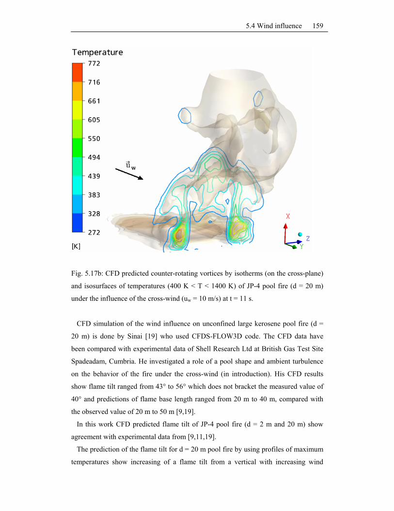
5.4 Wind influence
159
Fig. 5.17b: CFD predicted counter-rotating vortices by isotherms (on the cross-plane)
and isosurfaces of temperatures (400 K < T < 1400 K) of JP-4 pool fire (d = 20 m)
under the influence of the cross-wind (uw = 10 m/s) at t = 11 s.
CFD simulation of the wind influence on unconfined large kerosene pool fire (d =
20 m) is done by Sinai [19] who used CFDS-FLOW3D code. The CFD data have
been compared with experimental data of Shell Research Ltd at British Gas Test Site
Spadeadam, Cumbria. He investigated a role of a pool shape and ambient turbulence
on the behavior of the fire under the cross-wind (in introduction). His CFD results
show flame tilt ranged from 43° to 56° which does not bracket the measured value of
40° and predictions of flame base length ranged from 20 m to 40 m, compared with
the observed value of 20 m to 50 m [9,19].
In this work CFD predicted flame tilt of JP-4 pool fire (d = 2 m and 20 m) show
agreement with experimental data from [9,11,19].
The prediction of the flame tilt for d = 20 m pool fire by using profiles of maximum
temperatures show increasing of a flame tilt from a vertical with increasing wind

5 Results and discussions 160
velocity uw, from 20° for uw = 1.4 m/s to 70° for uw = 10 m/s whereas the tilt of 80° is
predicted when uw reaches 16 m/s.
The CFD predicted flame tilt and a flame drag by means of averaged data for
different wind velocities compared with calculated flame tilt and flame drag are
presented in Table 5.9. The results are obtained for each time step ∆t (e.g. ∆t = 0.1 s)
and averaged over the burning time of tb = 10 s.
The CFD predicted results agree well with the experimentally obtained photographs
[3,4,9,10,16,19] and calculated data (Table 5.9). The empirical correlations used for
comparison with CFD predicted flame tilt and a flame drag (Table 5.7 and 5.8) are
based on the experiments with gasoline and diesel pool fires [20] and small scale fires
[25].
Flame tilt
11
*w
b **ww
1 , for u < 1cosΘ =
,for u 1a (u )
(5.14a)
with *w w cu = u / u (5.14b)
and f fc v au (gm d / ρ ) (gm d / ρ )1/3 1/3 (5.14c)
where *wu is a wind velocity measured at height of 1.6 m;
Table 5.7: Empirical correlations [7] for calculation the flame tilt used in Eq. 5.14a.
Correlation a1 b1 Comments
AGA 1 – 0.5 measured on LNG pool fires [5]
Thomas 0.7 – 0.49 measured on wood fires [42]
Moorhouse 0.86 – 0.25 measured on large cylindrical LNG pool fires,
* *w wu = u (10) [44]
Muñoz 0.96 – 0.26 measured on gasoline and diesel pool fires [20]
Flame drag
1 11 d ev aw
d / d = c (Fr) (ρ / ρ ) . (5.15)

5.4 Wind influence
161
Table 5.8: Empirical correlations [25] for calculation the flame drag used in Eq. 5.15.
Correlation c1 d1 e1 Comments
- 1.6 0.061 0 conical flame
- 1.5 0.069 0 cylindrical flame
Sliepcevich 2.1 0.21 0.48
The correlation of Munoz (Table 5.7) is used for comparison with CFD predicted
flame tilt and the flame drag calculated with correlation of Sliepcevich (Table 5.8) is
compared with CFD predicted flame drag (Table 5.9). The CFD predicted flame tilts
(Table 5.9) agree with experimental and calculated data, except for d = 20 m JP-4
pool fire under the small wind velocity uw ≤ 1.4 m/s where calculation neglect the
flame tilt.
Table 5.9: Measured, calculated and CFD predicted flame tilt and a flame drag
d (m) uw
(m/s) Tilt (exp) Tilt (calc) Tilt (CFD) Drag (exp) Drag (calc)
Drag
(CFD)
2 4.5 60° 63° 60° 1.8 1.6 2.5
2 10 70° 72° 80° 2.0 1.6 2.6
2 16 70° 76° 80° 2.0 1.6 2.8
20 0.7 20° 0° 20° 1.1 1.0 1.1
20 1.4 20° 0° 20° 1.1 1.0 1.1
20 2.3 30° 20° 30° 1.5 2.0 1.8
20 4.5 40° 48° 50° 1.2 2.0 1.5
20 5.5 50° 52° 60° 2.0 2.0 1.6
20 7.2 70° 58° 60° 2.0 2.0 1.8
20 10 n.a. 63° 70° n.a. 2.0 2.0
20 16 n.a. 69° 80° n.a. 2.0 2.5
CFD over predicts flame drag in a case of d = 2 m JP-4 pool fire whereas for d = 20 m
agree with the experimental data. Calculated flame drag show constant value which
refers to the averaged value based on the experiments on small pool fires or large

5 Results and discussions 162
LNG fires [25] which can explain the discrepancy between calculated and CFD
predicted results.
5.4.2 Wind influence on surface emissive power (SEP), irradiance (E),
temperature, flow velocity
Wind influence on surface emissive power (SEP) and irradiance (E)
To illustrate the relationship between air flow and temperature field, SEP and
irradiance, the CFD simulations of JP-4 pool fires (d = 2 m and 20 m) under the
influence of cross wind with different wind velocities (uw = 1.4 m/s, 2.3 m/s, 4 m/s,
4.5 m/s, 10 m/s and 16 m/s) are performed.
The following flow processes can be found both in the simulated JP-4 pool fires
comparable with experiments on JP-4 and JP-8 pool fire [9,11,19].
Fig. 5.18: Measured [11] and CFD predicted irradiances E (∆y/d) at different relative
distances ∆y/d from the pool rim of a JP-4 pool fire (d = 2 m) under the influence of
cross wind with (uw = 4.5 m/s).

5.4 Wind influence
163
It is found that the wind causes significant radiation increase in the downwind
direction of a fire (Fig. 5.18, 5.19) and affects the radiation level slightly in the
upwind and cross-wind directions as it is observed in experiments [9,11]. CFD
predicted SEP and E downwind of the pool increases with wind speed and reaches a
maximum at the wind speed of about uw = 10 m/s which is close to the experimentally
[11] obtained value of 6.7 m/s ≤ uw ≤ 8.9 m/s and decreases at higher speeds. The
large value of SEP and E downwind of the fire is influenced also with the flame tilt.
Due to the smoke blockage, intense heating and improper viewing the radiation
measurements near the fire is difficult so the experimental results show radiation
measured at Δy/d ≥ 0.5 [11] (Fig. 5.18). This can explain the discrepancy between
predicted and measured E (∆y/d) at the closer distance to the pool rim (e.g. for ∆y/d ≤
0.5 on the Fig. 5.18).
Fig. 5.19: CFD predicted time-averaged irradiances E (∆y/d) at different relative
distances ∆y/d from the pool rim of a JP-4 pool fire (d = 20 m) under the influence of
the cross-wind with different wind velocities.

5 Results and discussions 164
Wind influence on temperature
Increasing the wind velocity up to e.g. uw = 10 m/s, due to the flame tilt and drag the
predicted maximum time averaged axial temperatures CFDmax,T of JP-4 pool fires are
found at larger relative distances y/d > 1 from the flame centerline as shown on Fig.
5.20-5.23.
In a case of JP-4 pool fire (d = 20 m), with increasing the wind velocity up to e.g. uw
= 10 m/s, the predicted maximum time averaged axial temperature CFDmax,T is found
at the axial distance x/d = 0.08 and radial distance Δy/d = 1 (y/d = 1.5) from the pool
rim.
CFD simulation shows that under the influence of the wind with uw = 10 m/s the fire
diameter (d = 20 m) extends for an additional d (Table 5.9, Fig. 5.22 and 5.23). On the
Fig. 5.23 is shown that the maximum time averaged axial temperature CFDmax,T is
found at the relative distance of y/d = 1.5 from the flame centerline which means that
the flame tilt from the vertical is about 70° and a flame drag is 2 (Tab. 5.9). At the
flame centerline the very high temperatures can still be found at a very low axial
distance from the pool (x/d = 0.025) (Fig. 5.23).
In the Fig. 5.20-5.21 CFD predicted isotherms and isosurfaces of temperatures (400
K < T < 1400 K) show instantaneous flame tilt and drag of JP-4 pool fire with d = 2 m
and 20 m under the wind velocity of uw = 4.5 m/s, compared with VIS images. It is
found that the maximum time averaged axial temperature CFDmax,T in a case of lower
wind condition is found at the relative distance of y/d = 2 and 1 (for d = 2 m and 20
m) from the flame centerline which means that the flame tilts from the vertical are
about 60° and 50° and the flame drags are 2.5 and 1.5 (for d = 2 m and 20 m) (Tab.
5.9).

5.4 Wind influence
165
(a)
(b)
Fig. 5.20: (a) CFD predicted isosurfaces of temperatures (400 K < T < 1400 K) and
(b) VIS image of a JP-4 pool fire (d = 2 m) under the influence of the cross-wind
(uw = 4.5 m/s).

5 Results and discussions 166
(a)
(b)
Fig. 5.21: (a) CFD predicted isosurfaces of temperature (400 K < T < 1400 K) and (b)
VIS image of a JP-4 pool fire (d = 25 m) under the influence of the cross-wind (uw =
4.5 m/s).

5.4 Wind influence
167
(a)
(b)
Fig. 5.22: CFD predicted (a) isotherms and (b) isosurfaces of temperatures (400 K ≤ T
≤ 1000 K) of JP-4 pool fire (d = 20 m) under the influence of the cross wind (uw = 10
m/s).

5 Results and discussions 168
Fig. 5.23: Time averaged axial temperature profiles at different radial distances y/d
from the flame axis of JP-4 pool fire (d = 20 m) under the cross-wind (uw = 10 m/s).
Wind influence on flow velocity
In the CFD simulations it is not found a significant increasing of the flame velocity
but it is predicted that the maximum flow velocity in a flame always follows the flame
tilt and it is found in a plume region (Fig. 5.24, 5.25).
The additional wind flow in a simulation influences the rotational velocities so the
vortex formation is more pronounced than in simulations without wind included even
if the RANS calculation and simplified chemistry (multistep chemical reaction) is
used.

5.4 Wind influence
169
(a)
(b)
Fig. 5.24: CFD predicted (a) instantaneous isotherms and flow field and (b)
isosurfaces of temperatures (400 K ≤ T ≤ 1000 K) of JP-4 pool fire (d = 20 m) under
the influence of the cross wind of uw = 7.2 m/s at t = 8 s.

5 Results and discussions 170
(a)
(b)
Fig. 5.25: CFD predicted (a) instantaneous isotherms and flow field and (b)
isosurfaces of temperatures (400 K ≤ T ≤ 1000 K) of JP-4 pool fire (d = 20 m) under
the influence of the cross wind of 16 m/s at t = 8 s.

5.5 Validation of CFD results
171
5.5 Validation of CFD results
The validation of the calculated fields and sizes, such as temperature, flow velocities,
thermal radiation and soot amount in large JP-4 pool flames contains several steps.
First is to use the images and profiles of the transient values to give the relationship
between the individual fields sizes (Chapter 5.1). Next step is to compare the
predicted time averaged temperatures with the measured data. The following is to
look at the transient thermal radiation such as incident radiation to the chosen area or
irradiances at the different distances from the pool rim (Chapter 5.2 and 5.3) to
discuss the influence of the flame dynamic on the thermal radiation from the fire.
Further step is to look into transient data of soot amount in large fires to explain the
influence on the thermal radiation. In the next step the CFD predicted time averaged
values of incident radiations and irradiances are compared with measurements or
empirical correlations to discussion about the strengths of the flame radiation and its
effect on neighboring objects. The simple juxtaposition of CFD simulations and
experiments can be strictly taken as a validation. Due to the lack of clear definitions
for validation and verification, this method is however a long time been considered
sufficient and is still very widespread. More recently, the desire is to identify more
accurate estimates for the experimental and numerical uncertainties. According to the
American Institute of Aeronautics and Astronautics (AIAA) is in the verification
examined whether an implemented model is suitable for the certain concept and if the
implemented model correctly solves its equations [108]. During the validation is
examined how accurately a model represents the part of the "real world", for which it
was developed.
For the quantitative evaluation of simulations in [108] different criteria are defined
to indicate the errors in relation to a size x. The error F(x) depends directly on the
calculated value ym (x) and the mean value ye (x) from the experiments from:
F(x) = ym (x) – ye (x). (5.16a)
The error is with a 90% probability in the field
0.05,f 0.05,fs(x) s(x)
F(x) t ,F(x) + tn n
(5.16b)
where s(x) is standard deviation. The distribution of t depends on the degrees of
freedom f = n – 1 for n of x.

5 Results and discussions 172
Oberkampf et.al gives also the criteria for the average and maximum error:
xum e
e u ex1avg 1
y (x) y (x)F 1= dx
y x x y (x)
(5.16c)
1
m ex x xue emax
y (x) y (x)F= max
y y (x)
(5.16d)
The highest value of size x is here with xu and with the lowest xl are described. An
average relative confidence indicator (CI) is calculated by:
1 1
xu0.05ν
e exuavg
tCI s(x)= dx
y y (x)(x x ) n (5.16e)
The maximum CI is calculated by:
1
xu0.05ν
e exmax
tCI s(x)= dx
y y (x)n
ˆ
ˆ (5.16f)
Using these equations the deviations of the simulation results from the experiment
can be quantitatively assessed. The knowledge of the measurements and their
associated uncertainties is necessary. It should also measurements of various working
groups and correlations be used but their uncertainties, however, generally are not
known. In this work a directly comparison of the CFD results with the measured data
is presented in a form of fields, profiles and time average values due to the reason that
at this time are still too little experimental data available.
In the following text validation of CFD results of temperature and SEP of JP-4 pool
fires is done by using global metric [108].
Calculation of uncertainties of the flame temperature and SEP
By using global metric (Eqs. (5.16a)-(5.16f)) the error is calculated for CFD predicted
T and SEP of JP-4 pool fire (d = 16 m) compared with experimental values from
Tab. 5.1 and Fig. 5.14. The results are shown in Tab. 5.10a,b.
CFD results in Tab. 5.10a,b show a good agreement with the measured values.
Averaged and maximal relative errors are small due to the large confidence interval
CI. Code validation needs more experimental data to decrease CI.

5.5 Validation of CFD results
173
Table 5.10a: Calculation of uncertainties of the time averaged temperature T of JP-4
pool fire (d = 16 m)
SAS (1M)*
Averaged relative error 0.14
Averaged relative confidence interval 0.89
Maximal relative error 0.79
Confidence interval of max. error 0.89
*CFD simulation is done by using SAS model and 1 million cell mesh
Table 5.10b: Calculation of uncertainties of the time averaged SEP of JP-4 pool fire
(d = 16 m)
SAS (1M)*
Averaged relative error 0.118
Averaged relative confidence interval 0.89
Maximal relative error 0.95
Confidence interval of max. error 0.89
*CFD simulation is done by using SAS model and 1 million cell mesh

5 Results and discussions 174

6. Conclusions
The following conclusions are summarized from the results:
1. CFD simulation on sooty, large, hydrocarbons pool fires develops to a powerful
method for a prediction of thermal radiation from the fire.
2. By CFD simulation it is possible to predict the SEPCFD as a function of time and
space. The “derived” quantity SEPCFD can be predicted by using following three
ways:
- Determination of an isosurface of constant temperature as a flame surface
- Integration over many distributions of incident radiation G along the z direction
through the flame
- By irradiance E(Δy/d, t) calculated by virtual wide angle radiometers defined at
the pool rim Δy/d = 0.
3. CFD simulation predicts also the time dependent irradiances CFD
E (Δy/d, t) and
time averaged CFD
E (Δy/d) by virtual radiometers at different horizontal distances
Δy/d from the pool rim.
4. A four-step discontinuity function for the effective absorption coefficient effæ
which considers the dissipative structures reaction zones, hot spots and soot
parcels is presented.
5. By CFD simulation it is possible to predict the flame tilt, drag, temperature, SEP
and irradiance of the pool fires under the wind influence.
6. For the successful CFD simulation it is necessary to use a detailed reaction
mechanism as flamelet models.
7. Further progress is focused on a reduction of CPU time e.g. by using of compute
cluster with higher performance.

6. Conclusions 176

References
[1] M. Hailwood, M. Gawlowski, B. Schalau, A. Schönbucher, Chem. Eng.
Technol. (2009), doi:10.1002/ceat.200800595.
[2] The Buncefield Investigation, Progress Report, February 2006,
www.buncefieldinvestigation.gov.uk/report.pdf.
[3] D. Göck, Experimentell fundierte Ballenstrahlungsmodelle zur Bestimmung von
Sicherheitsabständen bei großen Poolflammen flüssiger Kohlenwasserstoffe,
Dissertation, Universität Stuttgart, 1988.
[4] R. Fiala, D. Göck, X. Zhang, A. Schönbucher, Chem. Ing. Tech. 63 (1991) 760 –
761.
[5] K.S. Mudan, Prog. Energy Comb. Sci., 10 (1984) 59 – 80.
[6] F. P. Lees, Lee's Loss Prevention in the Process Industries (Eds. S. Mannan),
3th ed., Elsevier Butterworth-Heinemann, Burlington, MA, 2005.
[7] A. Schönbucher, Quellterme bei offenen Bränden von Flüssigkeiten und Gasen,
interner Bericht 2008.
[8] H. Koseki, Y. Iwata, Fire Technol., 36, 1 (2000) 24 – 38.
[9] S.R. Tieszen, V.F. Nicolette, L.A. Gritzo, J.K. Holen, D. Murray, J.L. Moya,
Vortical structures in pool fires: observation, speculation, and simulation, Sandia
report, SAND96-2607, November 1996.
[10] M. Gibbons, C. Devaud, E.J. Weckman, Behaviour of Pool Fires in a Crosswind:
Comparison of Experimental and Computational Results, CS/The Combustion
Institute, Halifax, May, 6 (2005).
[11] T. T. Fu, Fire technology, 10-1 (1974) 54 – 67.
[12] S.R. Tieszen, Annual Review of Fluid Mechanics (2001) 33 – 67.
[13] H. Koseki, Proc. of the 2nd Int. Symp. on Scale Modeling, Lexington 1997.
[14] K.B. McGrattan, H.R. Baum, A. Hamins, Thermal Radiation from Large Pool
Fires, Report NISTIR 6546, Fire Saftey Engineering Division Building and Fire
research Laboratory, 2000.
[15] K.B. McGrattan, H.R. Baum, R.G. Rehm, Fire Safety Journal (1998) 30 –161.
[16] M. Faghri, B. Sundén, Transport phenomena in fires, WIT press, Southampton,
Boston, 2008, ISBN: 978-1-84564-160-3.
References 178
[17] Y.L. Sinai, Fire Safety Journal 35 (2000) 51 – 61.
[18] V.F. Nicolette, L.A. Gritzo, Proc. of the 4th Int. Symp. on Fire Safety Science,
Ottawa (1994).
[19] Y.L. Sinai, Fire Safety Journal, 24, 1 (1995) 1 – 34.
[20] M. Muñoz, J. Arnaldos, J. Casal, E. Planas, Comb. Flame, 139 (2004) 263 –
277.
[21] M. Muñoz, E. Planas, F. Ferrero, J. Casal, J. Hazard. Mater. 144 (2007) 725 –
729.
[22] J.A. Fay, J. Hazard. Mater. B 136 (2006) 219 – 232.
[23] P.K. Raj, J. Hazard. Mater. 140 (2007) 280 – 292.
[24] P.K. Raj, Process Safety Progress 24, 3 (2005) 192 – 202.
[25] W.F.J.M. Engelhard in Methods for the Calculation of Physical Effects – The
Yellow Book (C.J.H. van den Bosch, R.A.P.M. Weterings (Eds.)), 3rd Ed., Part
2, 6.1-6.130, The Committee for the Prevention of Disasters, TNO, The Hague,
The Netherlands, 1997.
[26] M. Gawlowski, M. Hailwood, I. Vela, A. Schönbucher, Chem. Eng. Technol.
(2009), doi:10.1002/ceat.200800631.
[27] I. Vela, H. Chun K. B. Mishra, M.Gawlowski, P. Sudhoff, M. Rudolph, K.-D.
Wehrstedt, A. Schönbucher, Forschung Ingenieurwes., 2009, in press.
[28] C. Kuhr, CFD-Simulation der dynamischen Eigenschaften großer Kerosin- und
Heptan-Poolflammen, Dissertation, Universität Duisburg-Essen, 2008.
[29] K.A. Jensen, J.-F. Ripoll, A.A. Wray, D. Joseph, M. El Hafi, Combustion and
Flame 148 (2007) 263 – 279.
[30] C. Balluff, VIS-Ballenstrukturen und Oszillationen in Großflammen,
Dissertation, Universität Stuttgart, 1989.
[31] H. Chun, Experimentelle Untersuchungen und CFD-Simulation von DTBP-
Poolfeuern, BAM-Dissertationsreihe, Band 23, Berlin, 2007,
www.bam.de/de/service/publikationen/publikationen_medien/diss_23_vt.pdf
[32] C.H. Hottel: Certain Laws Covering Diffusive Burning of Liquids, F. Res. Abs.
And Rev., Vol. 3 (1959), 41 – 44.
[33] H.G. Werthenbach, Z. Forschung Technik Brandschutz 25 (1976) 57
[34] M. Hertzberg, Combustion and flame, 21 (1973) 195 – 209.

References
179
[35] A. Schönbucher, Massenabbrandraten und Lachengrößen bei
Flüssigkeitsbränden, presentation at 648. DECHEMA colloquium: “Entwicklung
von Quelltermen für Auswirkungsbetrachtungen”, Dechema Haus, Frankfurt am
Main, February 12. 2009.
[36] D. Burgess; A. Strasser; J. Grumer, Fire Res. Abst. Revs. 3 (1961) 177 – 192.
[37] J. Grumer, A. Strasser, T.A. Kubala, D.S. Burgess, Fire Res. Abstr. Rev. 3
(1961) 159
[38] D.S. Burgess, J.N. Murphy, M.G. Zabetakis, Bureau of mines Pittsburg PA
Safety Research Center, Repository Defense Technical Information Center
OAI-PMH Repository (United States) (2005)
[39] Babrauskas, V., Book Review. Fire Investigation, Fire Safety J. 40 (2005) 299
– 300
[40] V.I. Blinov and G.N. Khudiakov, Certain Laws Governing Diffusive Burning of
Liquids, Academiia Nauk, SSSR Doklady, Vol. 113, 1957, pp. 1094 – 1098.
[41] L. Orloff: Simplified Radiation Modeling of Pool Fires, Proc. Combust. Inst.,
Vol. 18 (1972) 549 – 583
[42] P.H. Thomas, The size of flames from natural fires, in: Proceedings of the 9th
International symposium on Combustion, The Combustion Institute, 1963, pp.
844 – 859.
[43] F.R. Stewart, Comb. Sci. Technol., Vol. 2 (1970) 203 – 212.
[44] J. Moorhouse, The Assessment of Major Hazards, Institution of Chemical
Engineers Symposium Series No. 71, Rugby (1982) 165 –180.
[45] G. Heskestad, Fire Safety J. 5 (1983) 103 –108
[46] E.E. Zukoski, B.M. Cetegen, T. Kubota, The Combustion Institute (1985) 361 –
366.
[47] B.J. McCaffrey, Purely Buoyant Diffusion Flames: Some Experimental Results,
Final Report, NBSIR 79-1910, 49 p, October 1979,
[48] J.R. Welker, C.M. Sliepcevich, Wind interaction Effects on Free Burning Fires,
Tech. Report #1441-3 to Office of Civil Defense of U.S. Bureau of Standards,
1967
[49] American Gas Association, LNG Safety Research Programm , Report IS 3-1,
1974
[50] E.J. Weckmann, A.B Strong, Comb. Flame 105 (1996) 245 – 266

References 180
[51] B.M. Cetegen, Combust. Sci. Tech. 123 (1997) 377 – 387
[52] S. Venkatesh, A. Ito, K. Saito, I.S. Wichman, 26th Symp. (Int.) Comb. (1996),
The Combustion Institute, Pittsburgh, 1437 -1443
[53] Y. Xin, J.P. Gore, K.B. McGrattan, R.G. Rehm, H.R. Baum, Comb. Flame 141
(2005) 329 – 335
[54] C. Kuhr, D. Opitz, R. Müller, A. Schönbucher, Proc. 10th Int. Symp. On Loss
Prevention and Safety Promotion in the Process Industries (2001), June 19-21,
Stockholm, Sweden, 1179 – 1188
[55] C. Kuhr, D. Opitz, R. Müller, A. Schönbucher, 5. Fachtagung Anlagen-,
Arbeitsund Umweltsicherheit (2000), Köthen, GVC.VDI-Gesellschaft
Verfahrenstechnik und Chemieingenieurwesen, 311 – 318
[56] C. Kuhr, Transiente Felder der Strömungsgeschwindigkeit, Vortizität und
Zirkulation in großen JP4-Poolflammen, Diplomarbeit, Universität Duisburg,
2000
[57] Koseki, H., Yumoto, T., Fire Technol. 24 (1988) 33-47
[58] E. Planas-Cuchi, J. Casal, J. Hazard. Mat. 62 (1998) 231 – 241.
[59] B.L. Bainbridge, N.R. Keltner, J. Hazar. Mater. 20 (1988) 21 – 40.
[60] J.J. Gregory, N.R. Keltner, R.J. Mata, J. Heat Transfer-Transactions of the
ASME 111 (1989) 446 – 454.
[61] K.B. McGrattan, H.R.Baum, A. Hamins, Thermal Radiation from Large Pool
Fires, Report NISTIR 6546, Fire Saftey Engineering Division Building and Fire
research
[62] M. Frenklach, D.W. Clary, W.C. Gardiner, S.E. Stein, 21st Symp. (Int.) Comb.
(1986), The Combustion Institute, Pittsburgh, 632 – 647.
[63] H. Bockhorn, T. Schäfer, in Soot Formation in Combustion (Bockhorn, H.
(Ed.)), 253 – 274, Springer Berlin, 1994.
[64] R. Dobbins, R.A. Fletcher, H.C. Chang, Comb. Flame 115 (1998) 285 – 298.
[65] H. Bockhorn, in Soot Formation in Combustion (Bockhorn, H. (Ed.)), 3–7,
Springer Berlin, 1994.
[66] U. Vandsburger, I. Kennedy, I. Glassman, Combust. Sci. Technol. 39 (1984)
263 – 285.
[67] A. Levy, 19th Symp. (Int.) Comb. (1982), The Combustion Institute, Pittsburgh,
1223 – 1242.

References
181
[68] J. Warnatz, U. Maas, R.W. Dibble, Verbrennung, 4. Auflage, Springer, Berlin
Heidelberg, 2006
[69] D. Bradley, G. Dixon-Lewis, S.E.D. Habik, E.M.J. Mushi, 20th Symp. (Int.)
Comb. (1984), The Combustion Institute, Pittsburgh, 931 – 940
[70] C.P. Fenimore, G.W. Jones, J. Phys. Chem. 71 (1967) 593 – 597
[71] F.P. Lees, in: S. Mannan (Ed.), Loss Prevention in the Process Industries, vol. 2,
3rd ed., Elsevier Butterworth-Heinmann, Burlington, MA, 2005.
[72] P.J. Rew, W.G. Hulbert, Development of Pool-Fire Thermal Radiation Model,
HSE Contract Research Report No. 96 / 1996, ISBN 0717610845
[73] W.K. Moser and C.F. Moser In: Fire and Forest Ecology: Innovative Silviculture
and Vegetation Management, (Eds.). Proceedings 21st Tall Timbers Fire Ecology
Conference on Fire and Forest Ecology, Tallahassee, Florida, 1998.
[74] L.T. Cowley, A.D. Johnson (1991), in [25]
[75] C.L. Beyler, in: P.J. DiNenno et al. (Eds.), SFPE Handbook of Fire Protection
Engineering. National Fire Protection Association, Quincy, MA, Section 3,
chap. 11, 3-268 to 3-314, 3 (2002).
[76] S. Mannan, Lee's Loss Prevention in the Process Industries, Vol. 1-3,
Elsevier Butterworth-Heinemann, 3 (2005).
[77] P.G. Seeger, GWF, Gas Erdgas 120 (1979) 25.
[78] A.N. Kolmogorov, J. Fluid Mech. 13 (1962) 82 – 85
[79] M. Griebel, T. Dornseifer; T. Neunhoeffer, Numerische Simulation in der
Strömungsmechanik, Vieweg, Braunschweig, 1995
[80] E.S. Oran, J.P. Boris, Numerical Simulation of Reactive Flow, 2nd Ed.,
Cambridge University Press, 2001
[81] R. Bryant, C. Womeldorf, E. Johnsson, T. Ohlemiller, Fire Mater. 27 (2003)
209 – 222
[82] I.G. Currie, Fundamental Mechanics of Fluids, 2nd Ed., McGraw-Hill, 1993
[83] ANSYS CFX 11.0 User Guide. AEA Technology, 2008, www.ansys.com
[84] ANSYS FLUENT 12 User Guide. AEA Technology, 2008, www.ansys.com
[85] A. Schönbucher: Thermische Verfahrenstechnik Grundlagen und
Berechnungsmethoden für Ausrüstungen und Prozesse, Springer-Verlag Berlin
Heidelberg, ISBN 3-540-42005-3 (2002)

References 182
[86] P.A. Libby, F.A. Williams, Turbulent Reacting Flows, Academic Press,
London, 1994
[87] J.H. Ferziger, M. Peric, Computational Methods for Fluid Dynamics, 2nd Edit.,
Springer, Berlin Heidelberg, 1997
[88] A.R. Paschedag, CFD in der Verfahrenstechnik, WILEY-VCH Weinheim, 2004
[89] Y. Egorov and F. Menter, Development and Application of SST-SAS
Turbulence, Advances in Hybrid RANS-LES Modelling in: Notes on Numerical
Fluid Mechanics and Multidisciplinary Design, Springer Berlin / Heidelberg,
Volume 97/2008, ISBN: 1612-2 909 (Print) 1060-0824 (Online)DOI:
10.1007/978-3-540- 77815-8
[90] E. Riesmeier, S. Honnet, N. Peters, Flamelet Modeling of Pollutant Formation
in a Gas Turbine Combustion Chamber using Detailed Chemistry for a
Kerosene Model Fuel, Proceedings of the 2002 Fall Technical Conference of the
ASME Internal Combustion Engine Division, ICE-Vol. 39 (2002) 149 – 157.
[91] N. Peters, G. Paczko, R. Seiser, K. Seshadri, Comb. Flame 128 (2002) 38 – 59.
[92] B.F. Magnussen, Modelling of NOx and Soot Formation by the Eddy Dissipation
Concept, Presented at the First Topic Oriented Technical Meeting,
International Flame Research Foundation, Amsterdam, The Netherlands, 1989
[93] P.A. Tesner, T.D. Snegirova, V. G. Knorre, Comb. Flame 17 (1971) 253 – 260
[94] K.M. Leung, R.P. Lindstedt, Jones, W.P., Comb. Flame 87 (1991) 289 – 305
[95] M. Fairweather, W.P. Jones, R.P. Lindstedt , Comb. Flame 89 (1992) 45 – 63
[96] J.H. Miller, W.G. Mallard, K.C. Smyth, 22st Symp. (Int.) Comb. (1986), The
Combustion Institute, Pittsburgh, 1057 – 1065
[97] J.H. Kent, H.G. Wagner, Comb. Flame 47 (1982) 53 – 65
[98] U. Vandsburger, I. Kennedy, I. Glassman, Combust. Sci. Technol. 39 (1984)
263 – 285
[99] F. Liu, H. Guo, G.J. Smallwood, Ö.L. Gülder, Combust. Theory Modelling 7
(2003) 301 – 315
[100] K.B. Lee, M.W. Thring, J.M. Beer, Comb. Flame 6 (1962) 137 – 145
[101] M. Griebel, T. Dornseifer, T. Neunhoeffer, Numerische Simulation in der
Strömungsmechanik, Vieweg, Braunschweig, 1995
[102] J.M. Chatris, J. Quintela, J. Folch, E. Planas, J. Arnaldos, J. Casal,
Comb.Flame 126 (2001) 1373 – 1383

References
183
[103] H. Koseki, G.W. Mulholland, T. Jin, Study on Combustion Property of Crude
Oil - A Joint Study Between NIST/CFR and FRI, Eleventh Joint Panel
Meeting of the UJNR Panel on Fire Research and Safety. Online im Internet:
http://www.mms.gov/tarprojects/026.htm, 2006
[104] J. Fröhlich: Large Eddy Simulation turbulenter Strömungen, Teubner-Verlag,
ISBN 10 3-8351-0104-8 (2006)
[105] K.M. Leung, R.P. Lindstedt, W.P. Jones, Comb. Flame 87 (1991) 289 –305
[106] C.L. Tien, K.Y. Lee, A.J. Stretton, Radiation heat transfer, in: SPFE handbook
of fire protection engineering, 2nd ed. Quincy, MA: NationalFire Protection
Association, 1995.
[107] C.W. Lautenberger, J.L. de Ris, N.A. Dembsey, J.R. Barnett, H.R. Baum, Fire
Safety J. 40 (2005) 141 – 176.
[108] W.L. Oberkampf, M.F. Barone, J. Comp. Phys. 217 (2006) 5 – 36.

References 184

Curiculum Vitae
Iris Vela, Dipl.-Phys.
Date of birth: 06/20/1969
Place of birth: Šibenik, Croatia
Citizenships: Croatian
Positions held
10/1991 – 05/1999 Student, University of natural sciences, Split, Croatia,
Department of physics and polytechnic,
Diploma thesis: "Hydrogen - the fuel of the future"
10/1999 – 06/2002 Student, Studies of computer sciences,
University of electrotechnic, Split, Croatia
Diploma thesis: "Reorganization of database”
Since
02/2003 Teaching and research assistant (Ph.D. Student), Department of
chemical engineering, University of Duisburg-Essen, Essen,
Germany
Research Area: “CFD simulation of large pool fires”
Head: Prof. Dr. Axel Schönbucher
Research experience
02/1994 – 03/1994 Praxis as a teaching assistant, Primary school “Spinut”, Split,
Croatia

02/1997 – 03/1997 Praxis as a teaching assistant, Primary school “Spinut”, Split,
Croatia
02/1997 – 03/1997 Praxis as a teaching assistant, High school III, Split, Croatia
02/2001 – 04/2001 Computer Engineer, Company „Automation-Split”, Split, Croatia
09/2002 – 02/2003 System Administrator, Company “Lemna Group“, Split, Croatia
02/2003 – 02/2009 Research and teaching assistant (Ph.D. student), Department of
chemical engineering, University of Duisburg-Essen, Essen,
Germany

Publications
[1] I. Vela, C. Kuhr, A. Schönbucher, CFD-Modeling of Large-Scale Kerosene Pool
Fires; Proceeding of the 11th International Symposium on Loss Prevention and
Safety Promotion in the Process Industry - Loss Prevention 2004, ISBN 80-02-
01574-6, 3143–3147
[2] H. Chun, I. Vela, K.-D. Wehrstedt, A. Schönbucher, Thermal radiation of di- tert-
butyl peroxide pool fires – experimental investigation and CFD simulation, J.
Hazard. Mater. (2009), doi:10.1016/j.jhazmat.2008.12.088
[3] M. Gawlowski, M. Hailwood, I. Vela, A. Schönbucher, Deterministic and
probabilistic estimation of acceptable separation distances – consequences for
industrial sites, Chem. Eng. Technol. 32 (2009) 182–198
[4] I. Vela, H. Chun, M. Gawlowski, K.B. Mishra, M. Rudolph, P. Sudhoff, K.-D.
Wehrstedt, A. Schönbucher, Vorhersage der thermischen Strahlung großer
Kohlenwasserstoff - und Peroxid- Poolfeuer mit CFD Simulation, Forsch.
Ingenieurwes. (2009), doi:10.1007/s10010-009-0094-3
[5] H. Chun, I. Vela, K.-D. Wehrstedt, A. Schönbucher, Mass burning rates and flame
heights of di-tert-butyl peroxide pool fires – experimental investigation and CFD
simulation, submitted to J. Hazard. Mater.
[6] I. Vela, M. Gawlowski, A. Schönbucher, The thermal radiation models OSRAMO
II, III for large hydrocarbon pool fires, submitted to J. Hazard. Mater.

Workshops, Symposia and Posters
[1] I. Vela, C. Kuhr, A. Schönbucher, Simulation of large open hydrocarbon fires with
cross-wind, Chemie Ingenieur Technik 76 (2004) 1353–1354
[2] I. Vela, C. Kuhr, M. Gawlowski, D. Göck, A. Schönbucher, The probabilistic
thermal radiation model OSRAMO II for large hydrocarbon pool fires, Proceedings
of the 31st International Symposium on Combustion 2006, 178, The Combustion
Institute, Pittsburgh
[3] I. Vela, M. Gawlowski, C. Kuhr, P. Sudhoff, A. Schönbucher, CFD simulation of
large hydrocarbon pool fires, Proceedings of the 31st International Symposium
on Combustion 2006, 177, The Combustion Institute, Pittsburgh
[4] I. Vela, C. Kuhr, A. Schönbucher, Scale Adaptive Simulation (SAS) der
Wärmestrahlung und der Rußkonzentrationen in einem turbulenten JP-8-
Poolfeuer, Chemie Ingenieur Technik 78 (2006) 1255–1256
[5] I. Vela, C. Kuhr, M. Gawlowski, D. Göck, A. Schönbucher, Das Modell
OSRAMO II zur Vorhersage der thermischen Strahlung großer Pool- und
Tankfeuer, 8. Fachtagung: Anlagen-, Arbeits- und Umweltsicherheit 2006, D02,
ISBN 3-936415-48-X
[6] I. Vela, M. Gawlowski, C. Kuhr, P. Sudhoff, A. Schönbucher, CFD study of
temperature and thermal radiation of large hydrocarbon pool fires, 8. Fachtagung:
Anlagen-, Arbeits- und Umweltsicherheit, 2006, P03, ISBN 3-936415-48-X
[7] I. Vela, M. Gawlowski, D. Göck, A. Schönbucher, Modelle der thermischen
Strahlung großer Feuer – Konsequenzen für Industriestandorte, Chemie Ingenieur
Technik 79 (2007) 1433–1434

[8] I. Vela, M. Gawlowski, P. Sudhoff, A. Schönbucher, CFD study about the
influence of absorption coefficients on thermal radiation in large JP-4 pool fires,
Chemie Ingenieur Technik 79 (2007) 1442
[9] M. Gawlowski, K.E. Kelly, I. Vela, P. Sudhoff, A. Schönbucher, LES einer n-
Hexan Tankflamme – Eine neue Validierungsmethode mit Interferogrammen,
Chemie Ingenieur Technik 79 (2007) 1444
[10] K.B. Mishra, K.-D. Wehrstedt, I. Vela, A. Schönbucher, Pool flames of organic
peroxides: experiments and CFD simulations, Proceedings of the 32st International
Symposium on Combustion 2008, 4P098, The Combustion Institute, Pittsburgh
[11] M. Gawlowski, K.E. Kelly, I. Vela, P. Sudhoff, A. Schönbucher, Temperature
measurements by real-time holographic interferometry in a tank fire – influence
of species composition, Proceedings of the 32st International Symposium on
Combustion 2008, 4P100, The Combustion Institute, Pittsburgh
[12] I. Vela, M. Hailwood, M. Gawlowski, P. Sudhoff, A. Schönbucher, Bisherige
Analyse des Buncefield-Ereignisses – Sind neue Konsequenzmodelle erforderlich,
9. Fachtagung: Anlagen-, Arbeits- und Umweltsicherheit, 2008, C01, Köthen,
Germany
[13] I. Vela, M. Gawlowski, P. Sudhoff, A. Schönbucher, CFD simulation of thermal
radiation from large JP-4 pool fires, 9. Fachtagung: Anlagen-, Arbeits- und
Umweltsicherheit, 2008, P04, Köthen, Germany
[14] K.B. Mishra, K.-D. Wehrstedt, I. Vela, A. Schönbucher, Pool flames of organic
peroxides: experiments and CFD simulations, 9. Fachtagung: Anlagen-, Arbeits-
und Umweltsicherheit, 2008, P08, Köthen, Germany