Embed Size (px)
Citation preview
8/10/2019 CFD Numerical simulation of a jet in crossflow..pdf
http://slidepdf.com/reader/full/cfd-numerical-simulation-of-a-jet-in-crossflowpdf 1/83
I S S N 0
2 4 9 - 6 3 9 9
I S R N I N
R I A / R R - - 5 6 3 8 - - F R + E N G
appor t
de r ec h erc he
Thème NUM
INSTITUT NATIONAL DE RECHERCHE EN INFORMATIQUE ET EN AUTOMATIQUE
Numerical simulation of a jet in crossflow.
Application to GRID computing.
Vanessa Mariotti,
Simone Camarri,Maria Vittoria Salvetti,
Bruno Koobus,
Alain Dervieux,
Hervé Guillard,
Stephen Wornom
N° 5638
Juillet 2005

8/10/2019 CFD Numerical simulation of a jet in crossflow..pdf
http://slidepdf.com/reader/full/cfd-numerical-simulation-of-a-jet-in-crossflowpdf 2/83
8/10/2019 CFD Numerical simulation of a jet in crossflow..pdf
http://slidepdf.com/reader/full/cfd-numerical-simulation-of-a-jet-in-crossflowpdf 3/83
Unité de recherche INRIA Sophia Antipolis
2004, route des Lucioles, BP 93, 06902 Sophia Antipolis Cedex (France)Téléphone : +33 4 92 38 77 77 — Télécopie : +33 4 92 38 77 65
Numerical simulation of a jet in crossflow. Application to
GRID computing.
Vanessa Mariotti∗,
Simone Camarri†,
Maria Vittoria Salvetti‡,
Bruno Koobus
§
,Alain Dervieux¶,
Hervé Guillard,
Stephen Wornom∗∗
Thème NUM — Systèmes numériquesProjet Smash
Rapport de recherche n° 5638 — Juillet 2005 — 80 pages
Abstract: This work describes the LES and hybrid RANS/LES simulations for a rounded jet issuing normally into a cross-flow, also known as jet in cross-flow (JICF). This test case
is particularly suitable to study the capability of LES and hybrid approaches because of the presence of both separated and non-separated boundary layer regions. Simulations areperformed for a jet to cross-flow velocity ratio R = 2 and a Re = 82000, based on thecross-flow velocity and the jet diameter. The simulations are carried out using a numericalsolver of 3D compressible flows, named AERO. Large scales coherent structures observed inexperimental flow visualisations are reproduced in both the simulations and the obtainedmean and turbulent statistics are compared to experimental data. LES simulations seemto follow in a better way the experimental results than LNS. In the second case, there isnot sufficiant mixing between jet and cross-flow and thus the jet bends less and a too largerecirculation bubble forms behind the jet. This test case has been chosen also because wecan split the domain in two different regions, the pipe and the cross-flow, with a limited
∗ Dipartimento di Ingegneria Aerospaziale, Università di Pisa, Via Caruso, 56122 Pisa, Italy
† Dipartimento di Ingegneria Aerospaziale, Università di Pisa, Via Caruso, 56122 Pisa, Italy‡ Dipartimento di Ingegneria Aerospaziale, Università di Pisa, Via Caruso, 56122 Pisa, Italy§ Université de Montpellier II, Département de Mathématiques, CC.051 34095 MONTPELLIER Cedex
5, France and INRIA¶ INRIA, 2004 Route des Lucioles, BP. 93, 06902 Sophia-Antipolis, France INRIA, 2004 Route des Lucioles, BP. 93, 06902 Sophia-Antipolis, France
∗∗ INRIA, 2004 Route des Lucioles, BP. 93, 06902 Sophia-Antipolis, France

8/10/2019 CFD Numerical simulation of a jet in crossflow..pdf
http://slidepdf.com/reader/full/cfd-numerical-simulation-of-a-jet-in-crossflowpdf 4/83
2 V. Mariotti S. Camarri M.V. Salvetti B. Koobus A. Dervieux H. Guillard S. Wornom
interface. This is a good characteristic in order to test GRID computing, which is anothergoal of this work. GRID computing is an alternative way to carry out parallel computationswith respect to the classical clusters or parallel computers. It consists in using computersallocated in different sites exchanging data between the sites through the web (Internet). Inthe present work, GRID computing is tested for both JICF and for the flow in a pipe.
Key-words: Large-eddy simulation, hybrid RANS/LES simulation, jet in crossflow, GRIDcomputing
INRIA
8/10/2019 CFD Numerical simulation of a jet in crossflow..pdf
http://slidepdf.com/reader/full/cfd-numerical-simulation-of-a-jet-in-crossflowpdf 5/83
Simulation numérique d’un jet en présence d’unécoulement latéral. Application au calcul parallèle
GRID.
Résumé : Ce rapport décrit la simulation LES et la simulation hybride LES/RANS d’un jet circulaire dans un écoulement latéral (JICF de l’expression anglaise jet in crossflow ).Ce cas test est bien adapté à l’étude et à la validation des approches LES et hybride, caril est caractérisé par la présence de couches limites ainsi que de structures tourbillonnairescomplexes issues de la séparation des couches limites. Les simulations ont été conduites pourune configuration caractérisée par un rapport entre la vitesse du jet et celle de l’écoulementlatéral R=2 et par un nombre de Reynolds Re=82000. Les simulations ont été effectuées en
utilisant un solveur numérique pour des écoulements compressibles 3D (AERO). Les cara-ctéristiques principales de l’écoulement ont été capturées avec les deux différentes approches,mais les résultats de la simulation LES sont en général en meilleur accord avec les donnéesexpérimentales que ceux de la simulation hybride. En effet, dans cette dernière simulation lemélange entre le jet et l’écoulement latéral n’est pas bien pris en compte. Par conséquent, ladéviation de la trajectoire du jet est moins importante que dans les expériences et on a unerégion de recirculation derrière le jet trop importante. Ce cas test a été choisi aussi parceque le domaine de calcul peut être divisé en deux parties, le tuyau et la chambre, ayant uneinterface limitée. Ceci est désirable pour l’application au calcul GRID, ce qui représenteun autre objectif de ce travail. Le calcul GRID est un calcul parallèle qui utilise des ordin-ateurs situés dans différents laboratoires, en échangeant les données parmi les différents sitesà travers le web (Internet). Dans ce travail, on utilise le calcul GRID pour la simulation duJICF et de l’écoulement dans un tuyeau, afin de donner une contribution à l’évaluation des
performances de cette approche de calcul parallèle.
Mots-clés : Simulation des grandes échelles, simulation hybride RANS/LES, jet en écoule-ment latéral, calcul parallèle GRID
8/10/2019 CFD Numerical simulation of a jet in crossflow..pdf
http://slidepdf.com/reader/full/cfd-numerical-simulation-of-a-jet-in-crossflowpdf 6/83
4 V. Mariotti S. Camarri M.V. Salvetti B. Koobus A. Dervieux H. Guillard S. Wornom
Contents
1 Introduction 6
2 Turbulent flows 72.1 Direct numerical simulation . . . . . . . . . . . . . . . . . . . . . . . . . . . . 72.2 Reynolds-Averaged Navier-Stokes Equations . . . . . . . . . . . . . . . . . . . 10
2.2.1 Standard k- model . . . . . . . . . . . . . . . . . . . . . . . . . . . . 112.3 Large Eddy Simulation . . . . . . . . . . . . . . . . . . . . . . . . . . . . . . . 12
2.3.1 SGS modeling . . . . . . . . . . . . . . . . . . . . . . . . . . . . . . . . 122.3.2 Filtered equations of the motion . . . . . . . . . . . . . . . . . . . . . 132.3.3 Smagorinsky’s model . . . . . . . . . . . . . . . . . . . . . . . . . . . . 152.3.4 Resolution requirements for LES . . . . . . . . . . . . . . . . . . . . . 162.3.5 Boundary conditions . . . . . . . . . . . . . . . . . . . . . . . . . . . . 16
2.4 Limited Numerical Scales . . . . . . . . . . . . . . . . . . . . . . . . . . . . . 17
3 AERO code 183.1 Set of governing equations . . . . . . . . . . . . . . . . . . . . . . . . . . . . . 183.2 Space discretization . . . . . . . . . . . . . . . . . . . . . . . . . . . . . . . . 19
3.2.1 Convective fluxes . . . . . . . . . . . . . . . . . . . . . . . . . . . . . . 203.2.2 Diffusive fluxes . . . . . . . . . . . . . . . . . . . . . . . . . . . . . . . 22
3.3 Boundary conditions . . . . . . . . . . . . . . . . . . . . . . . . . . . . . . . . 233.4 Time advancing . . . . . . . . . . . . . . . . . . . . . . . . . . . . . . . . . . . 23
3.4.1 Explicit time advancing . . . . . . . . . . . . . . . . . . . . . . . . . . 243.4.2 Implicit time advancing . . . . . . . . . . . . . . . . . . . . . . . . . . 24
3.5 Parallelization . . . . . . . . . . . . . . . . . . . . . . . . . . . . . . . . . . . . 253.5.1 Explicit time integration procedure . . . . . . . . . . . . . . . . . . . . 253.5.2 Implicit time integration procedure . . . . . . . . . . . . . . . . . . . . 25
4 Grid Computing 264.1 MecaGRID pro ject . . . . . . . . . . . . . . . . . . . . . . . . . . . . . . . . . 264.2 MecaGRID resources . . . . . . . . . . . . . . . . . . . . . . . . . . . . . . . . 264.3 Establishment of Grid: Globus and VPN . . . . . . . . . . . . . . . . . . . . . 264.4 Parallelism and message passing . . . . . . . . . . . . . . . . . . . . . . . . . 27
5 Jet in cross-flow. Flow dynamics and test-case configuration 295.1 Vortex system associated with the transverse jet . . . . . . . . . . . . . . . . 30
5.1.1 Class 1 structures . . . . . . . . . . . . . . . . . . . . . . . . . . . . . 31
5.1.2 Class 2 structures . . . . . . . . . . . . . . . . . . . . . . . . . . . . . 315.2 Flow configuration . . . . . . . . . . . . . . . . . . . . . . . . . . . . . . . . . 325.3 Mesh geometry . . . . . . . . . . . . . . . . . . . . . . . . . . . . . . . . . . . 335.4 LES validation test case . . . . . . . . . . . . . . . . . . . . . . . . . . . . . . 355.5 Boundary and initial conditions . . . . . . . . . . . . . . . . . . . . . . . . . . 36
INRIA
8/10/2019 CFD Numerical simulation of a jet in crossflow..pdf
http://slidepdf.com/reader/full/cfd-numerical-simulation-of-a-jet-in-crossflowpdf 7/83
Numerical simulation of a jet in crossflow. 5
6 Results of the LES simulation 416.1 Simulation parameters . . . . . . . . . . . . . . . . . . . . . . . . . . . . . . . 416.2 Reproduction of general flow characteristics . . . . . . . . . . . . . . . . . . . 42
6.2.1 Horseshoe vortex (HSV) . . . . . . . . . . . . . . . . . . . . . . . . . . 446.2.2 Counter-rotating vortex pair (CRVP) . . . . . . . . . . . . . . . . . . 466.2.3 Ring like vortices (RLV) . . . . . . . . . . . . . . . . . . . . . . . . . . 496.2.4 Upright vortices (URV) . . . . . . . . . . . . . . . . . . . . . . . . . . 49
6.3 Flow statistics . . . . . . . . . . . . . . . . . . . . . . . . . . . . . . . . . . . . 506.3.1 Mean velocities . . . . . . . . . . . . . . . . . . . . . . . . . . . . . . . 506.3.2 Turbulent kinetic energy . . . . . . . . . . . . . . . . . . . . . . . . . . 526.3.3 Turbulent shear stress . . . . . . . . . . . . . . . . . . . . . . . . . . . 54
7 Results of the LNS simulation 547.1 Simulation parameters . . . . . . . . . . . . . . . . . . . . . . . . . . . . . . . 547.2 Reproduction of general flow characteristics . . . . . . . . . . . . . . . . . . . 55
7.2.1 Horseshoe vortex (HSV) . . . . . . . . . . . . . . . . . . . . . . . . . . 597.2.2 Ring like vortices (RLV) . . . . . . . . . . . . . . . . . . . . . . . . . . 607.2.3 Counter-rotating vortex pair (CRVP) . . . . . . . . . . . . . . . . . . 607.2.4 Upright vortices (URV) . . . . . . . . . . . . . . . . . . . . . . . . . . 62
7.3 Flow statistics . . . . . . . . . . . . . . . . . . . . . . . . . . . . . . . . . . . . 627.3.1 Mean velocities . . . . . . . . . . . . . . . . . . . . . . . . . . . . . . . 627.3.2 Turbulent kinetic energy and turbulent shear stress . . . . . . . . . . . 67
8 Grid results 688.1 Computational resources . . . . . . . . . . . . . . . . . . . . . . . . . . . . . . 68
8.2 Pipe with 241K vertices . . . . . . . . . . . . . . . . . . . . . . . . . . . . . . 698.3 JICF with 398K vertices . . . . . . . . . . . . . . . . . . . . . . . . . . . . . . 73
9 Conclusions 76
RR n° 5638
8/10/2019 CFD Numerical simulation of a jet in crossflow..pdf
http://slidepdf.com/reader/full/cfd-numerical-simulation-of-a-jet-in-crossflowpdf 8/83
6 V. Mariotti S. Camarri M.V. Salvetti B. Koobus A. Dervieux H. Guillard S. Wornom
1 Introduction
The present work is part of two research projects: the first is aimed at developing and validat-ing numerical codes, based on LES (Large-Eddy Simulation) and hybrid RANS (Reynoldsaveraged Navier-Stokes)/LES approaches, in order to solve unsteady and separated fluiddynamic problems and is carried out in a collaboration between the University of Pisa andthe INRIA. The latter is the MecaGRID project and is aimed at testing the Globus Toolkit,a framework used for Grid Computing. The MecaGRID project is sponsored by the FrenchMinistry of Research through the ACI-GRID program 1 and it is a joint project betweenINRIA-Sophia Antipolis (France), CEMEF of the ENSMP (Ecole de Mines de Paris), locatedin Sophia Antipolis (France) and IUSTI (Institut Universitaire des Systèmes Thermiques etIndustriels), located in Marseille (France).
The interest in developing methodologies to simulate turbulent flows is due to the highcomputational cost of direct numerical simulation (DNS), which is, in most cases of practicalinterest, not affordable with the present computational resources. Indeed, due to the factthat the computational cost increases roughly with the 3rd power of the Reynolds number,DNS may be used only for low Reynolds numbers and simple geometries, as explained indetails in Section 2. An alternative to DNS is represented by the RANS (Reynolds AveragedNavier-Stokes) approach. With this method only the mean flow is directly simulated, whilethe fluctuations are taken into account through the Reynolds stress tensor. This termintroduces 6 new unknowns, and thus, some closure models, in our case the k- model (seeSection 2.2.1), have to be introduced to close the problem. This method leads to widelyreduced computational requirements, and this represents a big advantage in comparisonwith DNS, but it encounters accuracy problems if separated flows or recirculation bubbleshave to be simulated. An intermediate approach between DNS and RANS is represented
by Large-Eddy Simulation (LES), described in details in Section 2.3. It consists in filteringthe Navier-Stokes equations, simulating only the flow scales larger than the filter width andmodeling the small eliminated scales with appropriate models, in our case the Smagorinskymodel. Computationally, LES is less demanding than DNS, but is much more expensivethan RANS. The main advantage of LES in comparison with RANS is the capability of giving more accurate results for complex three-dimensional and time depending problems.The main drawback of the LES approach is represented by the still high computational cost.To have accurate results, indeed, fine meshes are required, especially near solid walls andthe mesh resolution requirements increase with the Reynolds number. In order to reducethe needed computational resources, hybrid RANS/LES approaches have been developed.One of these is based on Limited Numerical Scales (LNS), described in detail in Section2.4, which combines RANS and LES in a single model. The basic idea is to solve the LES
equations where the mesh is fine enough to give good results and RANS equations otherwise.In practice, a blending criterion between LES and RANS is used, which is based on the valuesof the corresponding eddy-viscosities.
1http://www.recherche.gouv.fr/recherche/aci/grid.htm
INRIA
8/10/2019 CFD Numerical simulation of a jet in crossflow..pdf
http://slidepdf.com/reader/full/cfd-numerical-simulation-of-a-jet-in-crossflowpdf 9/83
Numerical simulation of a jet in crossflow. 7
These approaches to turbulence are implemented in a numerical solver of 3D compressibleflows, named AERO, which was developed by INRIA (France) and University Colorado atBoulder (USA). It uses a mixed finite-element and finite-volume formulation for the spatialdiscretization on unstructured meshes made of tetrahedra; both implicit or explicit timeadvancing are available for the temporal discretization and it is parallelized using MPI.
As we have already pointed out, another goal of this work is to test the performance of Grid Computing within the MecaGRID project. Grid Computing extends older concepts of distributed computing, such as the classical parallel computing, but in contrast with oldersystems, Grid Computing makes easier the allocation of needs to resources. Information fromthe different sites, where the computers are located, are exchanged using the web (Internet).The global inter-communications are, indeed, slower than the local inter-communicationswhich use the local net. The main advantage of Grid Computing is the possibility of using
computers located in different sites and in this way to be able to use a large number of processors which otherwise will be only partially exploited.
To validate the LES and the hybrid LNS models, a rounded jet issuing normally intoa cross-flow, also known as jet in cross-flow configuration(JICF), has been simulated. Thisconfiguration has several practical applications because of its ability to mix rapidly withcross-flow and to introduce a controlled jet forced into the flow-field (i.e. injectors forcooling systems, exhaust of vehicles). It is interesting also from the basic research point of view because it is characterized by several vortical structures of different kind and dimension.Simulations are performed for a jet to cross-flow velocity ratio R = 2 and for a Reynoldsnumber Re = 82000, based on the cross-flow velocity and the diameter of the pipe. R = 2has been chosen because, for this velocity ratio value, the jet is able to push through theboundary layer of the cross-flow, thus the vortical structures form after the jet. The choiceof Re = 82000 is due to the presence of detailed experimental results carried out for thiscouple of parameters (R = 2 and Re = 82000) by Andreopoulos at al., Ref. [24]. Thepresence of both separated and non-separated flow regions is interesting for validate bothLES and LNS models.
For Grid Computing, this test case is also of interest. In particular, the area wherethe interface between the pipe and the cross-flow is located is quite small. Thus, if theinformation is exchanged only for this zone, the number of communications is reduced andone of the main problems of Grid Computing, i.e. the communication between sites locatedin different places, is partially overcome.
2 Turbulent flows
2.1 Direct numerical simulationThe accurate description of turbulent flow phenomena and their prediction are matter of primary concern for the solution of many engineering problems. Due to the absence of apredictive theory valid for all the different turbulent flows, the simulation of these phenomenais one of the main problems in Computation Fluid Dynamics.
RR n° 5638
8/10/2019 CFD Numerical simulation of a jet in crossflow..pdf
http://slidepdf.com/reader/full/cfd-numerical-simulation-of-a-jet-in-crossflowpdf 10/83
8 V. Mariotti S. Camarri M.V. Salvetti B. Koobus A. Dervieux H. Guillard S. Wornom
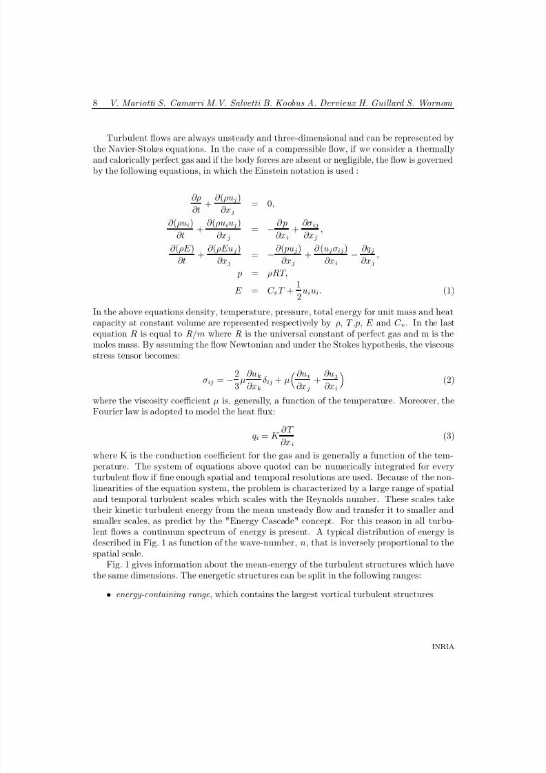
Turbulent flows are always unsteady and three-dimensional and can be represented bythe Navier-Stokes equations. In the case of a compressible flow, if we consider a thermallyand calorically perfect gas and if the body forces are absent or negligible, the flow is governedby the following equations, in which the Einstein notation is used :
∂ρ
∂t +
∂ (ρuj)
∂xj= 0,
∂ (ρui)
∂t +
∂ (ρuiuj)
∂xj= −
∂ p
∂xi+
∂σij
∂xj,
∂ (ρE )
∂t +
∂ (ρEuj)
∂xj= −
∂ ( puj)
∂xj+
∂ (ujσij)
∂xi−
∂q j∂xj
,
p = ρRT,
E = C vT + 1
2uiui. (1)
In the above equations density, temperature, pressure, total energy for unit mass and heatcapacity at constant volume are represented respectively by ρ, T , p, E and C v. In the lastequation R is equal to R/m where R is the universal constant of perfect gas and m is themoles mass. By assuming the flow Newtonian and under the Stokes hypothesis, the viscousstress tensor becomes:
σij = −2
3µ
∂uk
∂xkδ ij + µ
∂ui
∂xj+
∂uj
∂xi
(2)
where the viscosity coefficient µ is, generally, a function of the temperature. Moreover, theFourier law is adopted to model the heat flux:
q i = K ∂ T
∂xi(3)
where K is the conduction coefficient for the gas and is generally a function of the tem-perature. The system of equations above quoted can be numerically integrated for everyturbulent flow if fine enough spatial and temporal resolutions are used. Because of the non-linearities of the equation system, the problem is characterized by a large range of spatialand temporal turbulent scales which scales with the Reynolds number. These scales taketheir kinetic turbulent energy from the mean unsteady flow and transfer it to smaller andsmaller scales, as predict by the "Energy Cascade" concept. For this reason in all turbu-lent flows a continuum spectrum of energy is present. A typical distribution of energy is
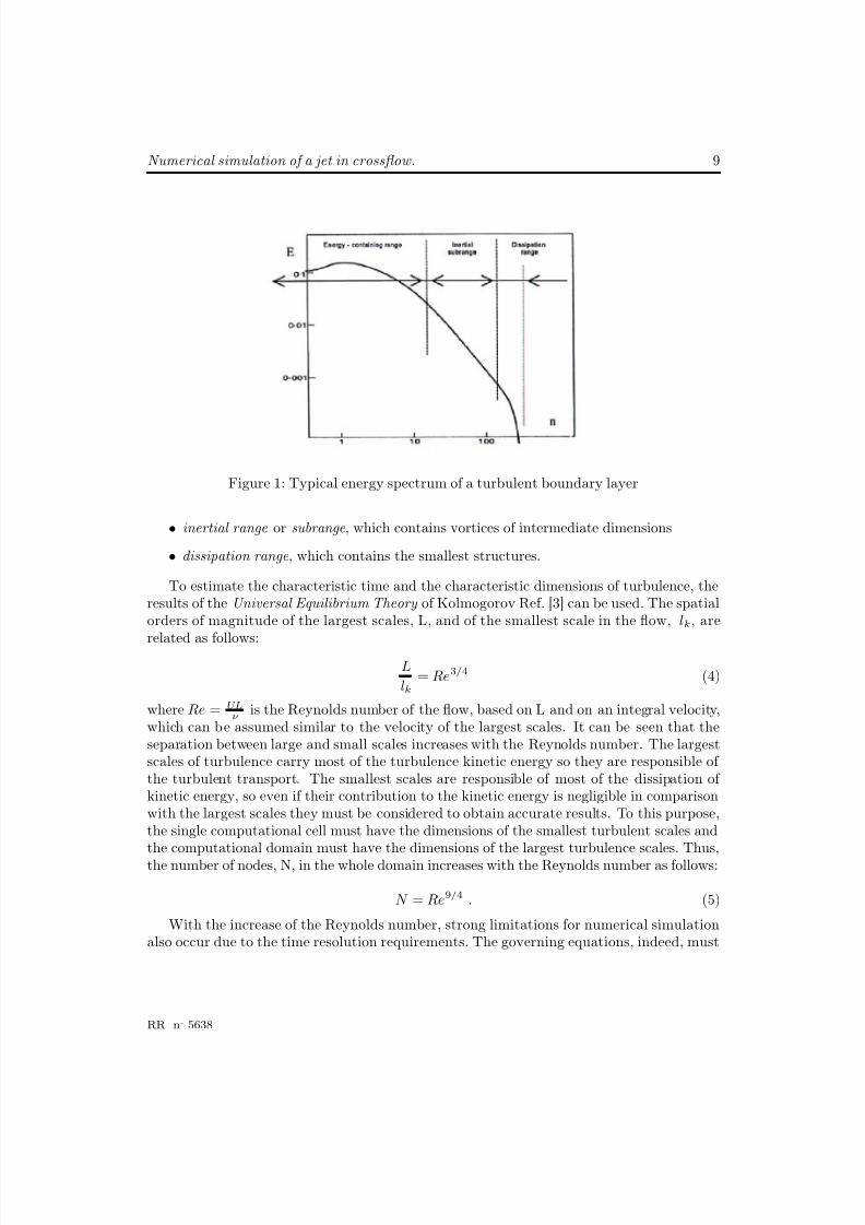
described in Fig. 1 as function of the wave-number, n, that is inversely proportional to thespatial scale.
Fig. 1 gives information about the mean-energy of the turbulent structures which havethe same dimensions. The energetic structures can be split in the following ranges:
• energy-containing range , which contains the largest vortical turbulent structures
INRIA
8/10/2019 CFD Numerical simulation of a jet in crossflow..pdf
http://slidepdf.com/reader/full/cfd-numerical-simulation-of-a-jet-in-crossflowpdf 11/83
Numerical simulation of a jet in crossflow. 9
Figure 1: Typical energy spectrum of a turbulent boundary layer
• inertial range or subrange , which contains vortices of intermediate dimensions
• dissipation range , which contains the smallest structures.
To estimate the characteristic time and the characteristic dimensions of turbulence, theresults of the Universal Equilibrium Theory of Kolmogorov Ref. [3] can be used. The spatialorders of magnitude of the largest scales, L, and of the smallest scale in the flow, lk, are
related as follows:L
lk= Re3/4 (4)
where Re = ULν
is the Reynolds number of the flow, based on L and on an integral velocity,which can be assumed similar to the velocity of the largest scales. It can be seen that theseparation between large and small scales increases with the Reynolds number. The largestscales of turbulence carry most of the turbulence kinetic energy so they are responsible of the turbulent transport. The smallest scales are responsible of most of the dissipation of kinetic energy, so even if their contribution to the kinetic energy is negligible in comparisonwith the largest scales they must be considered to obtain accurate results. To this purpose,the single computational cell must have the dimensions of the smallest turbulent scales andthe computational domain must have the dimensions of the largest turbulence scales. Thus,the number of nodes, N, in the whole domain increases with the Reynolds number as follows:
N = Re9/4 . (5)
With the increase of the Reynolds number, strong limitations for numerical simulationalso occur due to the time resolution requirements. The governing equations, indeed, must
RR n° 5638
8/10/2019 CFD Numerical simulation of a jet in crossflow..pdf
http://slidepdf.com/reader/full/cfd-numerical-simulation-of-a-jet-in-crossflowpdf 12/83
10 V. Mariotti S. Camarri M.V. Salvetti B. Koobus A. Dervieux H. Guillard S. Wornom
be advanced for a global time interval, ∆T c, of the order of the largest temporal scales, T c,and the temporal step must be small enough to capture all the small temporal scales, of theorder of tk. The ratio between the largest and the smallest temporal scale is the following:
T ctk
= Re1/2 (6)
so if the global step is constant the number of temporal steps needed to cover all the range∆T c rise quickly with the increase of the Reynolds number.
The huge computational resources needed to directly simulate turbulent flows at highReynolds numbers are not affordable. For this reason, the direct numerical simulation(DNS) is only used for low Reynolds number and simple geometries. On the other hand theinformation which can be obtained in DNS, is much larger than what is required in industrial
or engineering problems. Due to this, other simplified models were developed in order toobtain the required information at a significantly reduced computational cost. ReynoldsAveraged Navier-Stokes (RANS), Large Eddy Simulation (LES) and Limited NumericalScales (LNS) are examples of these models.
It is important to stress that, unlike LES, RANS and LNS, DNS gives results that arefree of errors due to empirical assumptions about intrinsic turbulent physics and producesinformation about turbulence useful to devise and validate turbulent models for the closure of RANS and LES. Thus, DNS plays an important role for the industrial numerical simulation,although indirect.
2.2 Reynolds-Averaged Navier-Stokes Equations
In order to avoid the use of DNS and thus to avoid the solution of the complete system of Eqs. 1, the first alternative model proposed was based on statistical approach and is known asReynolds Averaged Navier-Stokes model (RANS). This method was introduced by Reynoldsand is based on the idea that the characteristic times of the averaged flow are much longerthan those of the turbulent structures. Thus, too small integration steps are not needed toresolve the mean flow and, if only the averaged flow is considered, the spatial discretizationshould capture only the gradients of the average motion. The unknown quantities of theproblem are the flow statistical quantities and only the mean flow is simulated where "mean"usually stands for the time-averaged flow. The equations governing the flow statisticalquantity are obtained by applying appropriate averaging, often time average, to the Navier-Stokes equations. If averaging is carried, each variable of the problem can be decomposedas follows:
x = x + x
(7)
where x and x stand for the mean value and the fluctuating part of the generic quantity,respectively. If we substitute the decomposition (7) in the Navier-Stokes equations and weapply the time-average we obtain, for an incompressible flow, the following classical set of RANS equations for the mean flow, where the Einstein notation is used:
INRIA
8/10/2019 CFD Numerical simulation of a jet in crossflow..pdf
http://slidepdf.com/reader/full/cfd-numerical-simulation-of-a-jet-in-crossflowpdf 13/83
Numerical simulation of a jet in crossflow. 11
∂ uj
∂xj= 0 ,
∂ ui
∂t +
∂ (ρuiuj)
∂ xj= −
1
ρ
∂ p
∂ xi+ ν
∂ 2ui
∂xixj−
∂
∂xj(ρ(u
iu
j)) . (8)
The equations for the averaged motion of a turbulent, Newtonian, incompressible floware formally identical to the Navier-Stokes equations with a new term that is made by theaveraged products of the velocity fluctuations. Those terms have the dimensions of a shearper unit of density and can be collected in a symmetrical tensor, known as Reynolds stresstensor, which represents the effects of fluctuations on the mean flow; its components are as
follows:
R(t)ij = −ρu
iu
j . (9)
In order to close the problem, the Reynolds stress tensor must be modeled as a functionof the mean flow. The number of existing models is huge and their complexity is variable.Due to the conceptual difficulty in modeling the Reynolds stress tensor, it is accepted thatit is impossible to find a model of general validity. Moreover there are class of flows, i.e.flows with massive separations or dominated by unsteady phenomena, for which the RANSmodels are not accurate enough and may be significantly sensitive to the boundary conditionsimposed for the turbulent quantities, which are sometimes difficult to be assigned.
2.2.1 Standard k- model
The standard k- model, proposed by Jones and Launder, Ref. [5], belongs to the class of the eddy viscosity models. In this models the following constitutive equation is applied, inanalogy with the modeling equation for the viscous stress tensor in Newtonian fluids:
Rij = µt P ij −
2
3 ρkδ ij = µt
∂ ui
∂xj+
∂ uj
∂xi−
2
3∂ ulxlδ ij
(10)
where µt is the turbulent eddy viscosity and δ ij is the Kronoecker symbol. Using the Eq.(10), the closure of the model is reduced to assign the eddy viscosity µt as a function of theaveraged flow field. In the k- model the eddy viscosity, µt, is defined as follows:
µt = C µk2
(11)
where C µ is a free constant usually equal to 0.09, k = u
ju
j is the turbulent kinetic energy
and = 2ν ∂u
i
∂xj
∂u
i
∂u
i
is the turbulent dissipation rate. The spatial distribution of k and is
estimated by solving the following transport equation:
RR n° 5638
8/10/2019 CFD Numerical simulation of a jet in crossflow..pdf
http://slidepdf.com/reader/full/cfd-numerical-simulation-of-a-jet-in-crossflowpdf 14/83
12 V. Mariotti S. Camarri M.V. Salvetti B. Koobus A. Dervieux H. Guillard S. Wornom
ρ∂k
∂t + ρuj
∂k
∂xj= Rij
∂ ui
∂xj− ρ +
∂
∂xj
µ +
µt
σk
∂
∂xj
,
ρ∂
∂t + ρuj
∂
∂xj= C 1
kRij
∂ ui
∂xj− C 2ρ
2
k +
∂
∂xj
µ +
µt
σ
∂
∂xj
(12)
where C 1, C 2, σk and σ are the model parameters and usually are set as follow:
C 1 = 1.44 C 2 = 1.92 σk = 1.0 σ = 1.3 .
2.3 Large Eddy Simulation
The large-eddy simulation approach (LES) is intermediate between DNS, where all fluctu-ations are resolved, and the statistical simulations based on RANS, where only the meanflow is resolved. In LES the severe Reynolds number restrictions of DNS are bypassed bydirectly simulating the large scales (GS) only and supplying the effect of the missing smallscales (SGS) by a so-called sub-grid model. This is obtained by filtering the Navier-Stokesequations in space, in order to eliminate the flow fluctuations smaller then the filter size.In this way, the new unknowns of the problem become the filtered flow variables. Like forRANS, due to the non-linearity of the original problem, the new equations contain additionalunknown terms, the so-called sub-grid scale (SGS) terms, representing the effect of the elim-inated small scales on the filtered equations. In order to close the problem, these terms mustbe modeled, but, due to the fact that the small unresolved scales are often simpler in naturethat the inhomogeneous large motions, since they do not significantly depend on the large
scale motion, rather simple closure models may work well for many applications. Anotheradvantage of this method is the possibility of directly simulating the largest scales, which areusually more interesting from the engineering point of view. Computationally, LES clearlyis less demanding than DNS, but in general much more expensive than RANS. The reason isthat, independent by the problem to be solved, LES always requires fully three-dimensionaland time-dependent calculations even for flows which are two- or one-dimensional in themean. Moreover LES, like DNS, needs to be carried out for long periods of time to obtainstable and significant statistics. For these reasons, LES should provide best results for theanalysis of complex three-dimensional and time-dependent problems where RANS frequentlyfails. The utilization of LES for engineering problem is not yet very extensive, but in recentyears the interest in this method has largely increased.
2.3.1 SGS modelingThe energy-carrying large scales structures (GS) mainly contribute for the turbulent trans-port and the dissipative small scale motions (SGS) carry most of the vorticity and act asa sink of turbulent kinetic energy. For high Reynolds numbers the dissipative part of thespectrum becomes clearly separated from the low wave-number range, in a way shown by
INRIA
8/10/2019 CFD Numerical simulation of a jet in crossflow..pdf
http://slidepdf.com/reader/full/cfd-numerical-simulation-of-a-jet-in-crossflowpdf 15/83
Numerical simulation of a jet in crossflow. 13
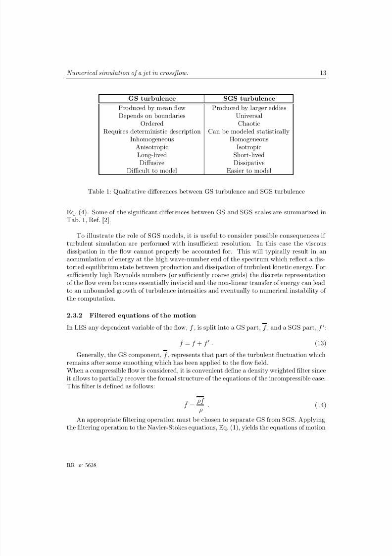
GS turbulence SGS turbulenceProduced by mean flow Produced by larger eddiesDepends on boundaries Universal
Ordered ChaoticRequires deterministic description Can be modeled statistically
Inhomogeneous HomogeneousAnisotropic IsotropicLong-lived Short-livedDiffusive Dissipative
Difficult to model Easier to model
Table 1: Qualitative differences between GS turbulence and SGS turbulence
Eq. (4). Some of the significant differences between GS and SGS scales are summarized inTab. 1, Ref. [2].
To illustrate the role of SGS models, it is useful to consider possible consequences if turbulent simulation are performed with insufficient resolution. In this case the viscousdissipation in the flow cannot properly be accounted for. This will typically result in anaccumulation of energy at the high wave-number end of the spectrum which reflect a dis-torted equilibrium state between production and dissipation of turbulent kinetic energy. Forsufficiently high Reynolds numbers (or sufficiently coarse grids) the discrete representationof the flow even becomes essentially inviscid and the non-linear transfer of energy can lead
to an unbounded growth of turbulence intensities and eventually to numerical instability of the computation.
2.3.2 Filtered equations of the motion
In LES any dependent variable of the flow, f , is split into a GS part, f , and a SGS part, f :
f = f + f . (13)
Generally, the GS component, f , represents that part of the turbulent fluctuation whichremains after some smoothing which has been applied to the flow field.When a compressible flow is considered, it is convenient define a density weighted filter sinceit allows to partially recover the formal structure of the equations of the incompressible case.
This filter is defined as follows:
f = ρf
ρ . (14)
An appropriate filtering operation must be chosen to separate GS from SGS. Applyingthe filtering operation to the Navier-Stokes equations, Eq. (1), yields the equations of motion
RR n° 5638
8/10/2019 CFD Numerical simulation of a jet in crossflow..pdf
http://slidepdf.com/reader/full/cfd-numerical-simulation-of-a-jet-in-crossflowpdf 16/83
14 V. Mariotti S. Camarri M.V. Salvetti B. Koobus A. Dervieux H. Guillard S. Wornom
of the GS flow field. Like in RANS the filtering of the non linearities is of particular interestsince it gives rise to additional unknowns terms. For LES of compressible flows, the filteredform of the equations of motion for a thermally and calorically perfect gas is the following:
∂ρ
∂t +
∂ (ρuj)
∂xj= 0
∂ (ρui)
∂t +
∂ (ρuiuj)
∂xj= −
∂ p
∂xi+
∂ (µ P ij)
∂xj−
∂M (1)ij
∂xj+
∂M (2)ij
∂xj
∂ (ρ E )
∂t +
∂ [(ρ E + p)uj
∂xj=
∂ (ujσij)
∂xi−
∂ q j∂xj
+ ∂
∂xj
Q(1)
j + Q(2)j + Q(3)
j
(15)
In the momentum equation the sub-grid terms are represented by the terms M (i)
ij which canbe defined as follows:
M (1)ij = ρuiuj − ρuiuj (16)
M (2)ij = µP ij − µ P i j (17)
and
P ij = −2
3S kkδ ij + 2S ij (18)
where S ij is the strain rate tensor defines as:
S ij = 1
2
∂ui
∂xj+
∂uj
∂si
. (19)
M (1)ij takes into account the momentum transport of the sub-grid scales and M
(2)ij rep-
resents the transport of viscosity due to the sub-grid scales fluctuations.
In the energy equation the sub-grid term are represented by the terms Q(i)j which can
be defined as follows:
Q(1)j =
ui
ρ E + p
− ui(ρE + p)
(20)
Q(2)j = µP ijuj− µ P ij uj (21)
Q(3)j = K
∂ T
∂xj− K
∂ T
∂xj(22)
Q(1)j represents three distinct physical effects:
INRIA
8/10/2019 CFD Numerical simulation of a jet in crossflow..pdf
http://slidepdf.com/reader/full/cfd-numerical-simulation-of-a-jet-in-crossflowpdf 17/83
Numerical simulation of a jet in crossflow. 15
• the transport of energy E due to small scale fluctuations;
• the change of the internal energy due to the sub-grid scale compressibility
p∂uj
∂sj
;
• the dissipation of energy due to sub-grid-scale motions in the pressure field
uj∂p∂xj
;
Q(2)j takes in account the dissipative effect due to the sub-grid scale transport of viscosity;
Q(3)j takes in account the heat transfer caused by the motion of the neglected sub-grid scales.
2.3.3 Smagorinsky’s model
The Smagorinsky model is an example of closure models. We assume that low compressibility
effects are present in the SGS fluctuations and that heat transfer and temperature gradientsare moderate. The retained SGS term in the momentum equation is thus the classical SGSstress tensor:
M ij = ρuiuj − ρuiuj (23)
where the over-line denotes the grid filter and the tilde the density-weighted Favre filter( f = (ρf )/ρ). The isotropic part of M ij can be neglected under the assumption of lowcompressibility effect in the SGS fluctuations. The deviatoric part, T ij , may be expressed byan eddy viscosity term, in accordance with the Smagorinsky model extended to compressibleflow:
T ij = −2µsgsS ij − 13 S kk, (24)
µsgs = ρC s∆2|S |. (25)
where S ij is the resolved strain tensor, µsgs is the SGS viscosity, ∆ is the filter width, C s
is a constant which must be assigned a priori and |S | =
S ij S ij . The width of the filter is
defined for every grid elements, l , as follows:
∆(l) = maxi=1,...,6(∆(li)) (26)
where ∆(l)i is the length of the i-th side of the l-th element, so ∆(l) is the length of the
largest edge.
In the energy equation the effect of the SGS fluctuations has been modified by the intro-duction of a constant SGS Prandtl number to be assigned a priori:
P rsgs = C pµsgs
K sgs(27)
RR n° 5638
8/10/2019 CFD Numerical simulation of a jet in crossflow..pdf
http://slidepdf.com/reader/full/cfd-numerical-simulation-of-a-jet-in-crossflowpdf 18/83
16 V. Mariotti S. Camarri M.V. Salvetti B. Koobus A. Dervieux H. Guillard S. Wornom
where K sgs is the SGS conductivity coefficient and it takes into account the diffusion of total energy caused by the SGS fluctuation. In the filtered energy equation, the term K sgsis added to the molecular conductivity coefficient.
Another limit for LES is due to the assumption frequently done in SGS models of takingthe cut-off of the filter in the inertial range, so very high computational requirements areneeded.
2.3.4 Resolution requirements for LES
The SGS effects in a turbulent flow depend qualitatively and quantitatively on the width of the filter function applied. Generally the filter width should be as large as possible in orderto minimize the computational needs of a simulation, but larger filter width gives rise to amore complex SGS turbulence. For this reason a compromise should be found.
2.3.5 Boundary conditions
LES simulation are generally significantly costly as regards both CPU and memory require-ments, especially when high Reynolds numbers and solid walls are simulated. The gridrefinement required in the near wall region has severely slowed the development of LES forflows of practical interest. For this reason several ways to treat the boundary conditions areintroduced. The proposed approaches to do this can be divided in two classes:
• near wall resolution method,
• near wall modeling method.
The near wall resolution method was the first method to be used and consists in decreas-ing the filter width to zero at the boundaries. In this way the important flow features nearthe boundary are captured, but this method has high computational cost since it requiresa very fine mesh near the walls. The near wall modeling method, instead, group togetherall the techniques aimed at keeping the grid coarse in the near wall region to reduce thecomputational cost. In particular those models can be classified in:
• wall law methods,
• two-layer approaches.
The wall-law methods use algebraic functions (wall-law) to reconstruct the velocity profilenear the wall where the fluid resolution is poor. The methods of this class differ in the type of
wall-law used and in the way in which the wall-law is employed to provided an approximateset of boundary conditions.The two-layer approach, instead, consists in resolving a set of equations in the near-wallregion derived from Navier-Stokes equations for turbulent attached boundary conditions.These methods can differ in the set of simplified solved equations.
INRIA
8/10/2019 CFD Numerical simulation of a jet in crossflow..pdf
http://slidepdf.com/reader/full/cfd-numerical-simulation-of-a-jet-in-crossflowpdf 19/83
Numerical simulation of a jet in crossflow. 17
2.4 Limited Numerical Scales
While LES is an increasingly powerful tool for unsteady turbulent flow prediction, it is stillprohibitively expensive. To bring LES closer to becoming a design tool, hybrid RANS/LESapproaches have been developed. One of these is based on Limited Numerical Scales (LNS)which combines RANS and LES in a single modeling framework. This approach has theadvantage of being particularly easy to implement in existing codes. In LNS the Reynoldstensor is modeled by an eddy-viscosity which is obtained by taking the minimum valuebetween the ones given respectively by RANS k- model and by the LES Smagorinskymodel. This allows the LES approach to be used where the grid resolution is adequate forresolving the largest turbulence scales, while the RANS approach is used where the grid isnot sufficiently refined. This model, as all the hybrid models, is mainly based on empiricism.Since very few applications of LNS are presented in the literature, it lacks validation to bereliably used in industry.
We can assume to use the k-, see Section 2.2.1, for the closure of the RANS equations,in which the Reynolds stress tensor is modeled as shown in Eq. 10. Thus, the LNS equationsare obtained from the RANS ones by replacing the Reynolds stress tensor, Rij , with the Lij
tensor which is equal to Rij multiplied by a blending function , α:
Lij = αRij (28)
The blending function α varies in space and time and in the LNS model proposed by Batten,Ref. [6], is defined as follows:
α = minµs
µt, 1
(29)
where µs is the SGS viscosity obtained from LES closures and µt is the turbulent viscosityobtained from RANS closures. If the Smagorinsky model is adopted the SGS viscosity isdefined as follows, see Section 2.3.3:
µs = ρC s∆2
S ij S ij (30)
The set of LNS equations is the follows:
∂ ρ
∂t +
∂ (ρui)
∂xi= 0,
∂ (ρui)
∂t +
∂ (ρuiuj)
∂xj
= − ∂ ¯ p
∂xi
+ ∂ (σij + Lij)
∂xj
,
∂ E
∂t +
∂ uj( E + ¯ p)
∂xj=
∂ uiσij
∂xj+
∂ uiLij
∂xj+
∂
∂xj
αµt
σk
∂k
∂xj+
∂
∂xj
C pP r
(µ + αµt) ∂ T
∂xj
RR n° 5638
8/10/2019 CFD Numerical simulation of a jet in crossflow..pdf
http://slidepdf.com/reader/full/cfd-numerical-simulation-of-a-jet-in-crossflowpdf 20/83
18 V. Mariotti S. Camarri M.V. Salvetti B. Koobus A. Dervieux H. Guillard S. Wornom
∂ (ρk)∂t
+ ∂ ρujk∂xj
= ∂ ∂xj
µ + αµt
σk
∂k∂xj
+ Lij∂ ui
∂xj− ρ,
ρ
∂t +
ρuj
∂xj=
∂
∂xj
µ +
αµt
σ
∂
∂xj
+ C 1
k
Lij
∂ ui
∂xj− C 2ρ
2
k . (31)
3 AERO code
In this section the main features of the numerical method are described.
3.1 Set of governing equations
In the AERO code the Navier Stokes equations are numerically normalized with the following
reference quantities:
• Lref =⇒ characteristic length of the flow,
• U ref =⇒ velocity of the free-stream flow,
• ρref =⇒ density of the free-stream flow,
• µref =⇒ molecular viscosity of the free-stream flow.
The flow variables can be normalized with the reference quantities as follows:
ρ∗ = ρ
ρref
u∗j = uj
U ref
p∗ = p
U ref pref
E ∗ = E
ρref U 2ref µ∗ =
µ
µref t∗ = t
Lref
U ref . (32)
The non-dimensional form of the Navier Stokes equations can be obtained substitutingthe reference quantities Eq. (32) in the set of equations described in Eq. (1) and is quotedin the following:
∂ρ∗
∂t∗ +
∂ (ρ∗u∗j )
∂x∗j= 0
∂ (ρ∗
u∗
i )∂t∗
+ ∂ρ∗
u∗
i u∗
j
∂x∗j= −∂p
∗
∂x∗i+ 1
Re∂σ
∗
ij
∂x∗j
∂ (ρ∗E ∗)
∂t∗ +
∂ (ρ∗E ∗u∗j )
∂x∗j= −
∂ ( p∗u∗j)
∂x∗j+
1
Re
∂ (u∗jσ∗ij)
∂x∗i−
γ
RePr
∂
∂x∗
j
µ∗
E ∗ − 1
2u∗ju∗j
(33)
INRIA
8/10/2019 CFD Numerical simulation of a jet in crossflow..pdf
http://slidepdf.com/reader/full/cfd-numerical-simulation-of-a-jet-in-crossflowpdf 21/83
Numerical simulation of a jet in crossflow. 19
where the Reynolds number, Re = U ref Lref /ν , is based on the references quantities, U ref and Lref , the Prandlt number, Pr, can be assumed constant for a gas and equal to:
P r = C pµ
k (34)
and γ = C p/C v is the ratio between the specific heats at constant pressure and volume. Alsothe constitutive equations for the viscous stresses and the state equations may be writtenin non-dimensional form as follows:
σ∗ij = −2
3µ∗∂u∗
k
∂x∗
k
δ ij
+ µ∗∂u∗
i
∂x∗j+
∂u∗
j
∂x∗
i
p∗ = (γ − 1)ρ∗E ∗ − 1
2
u∗ju∗j . (35)
In order to rewrite the governing equations in a compact form more suitable for thediscrete formulation, we group together the unknown variables in the W vector:W = (ρ, ρu, ρv, ρw, ρE )T .If we define the two vectors, F and V as function of W, as follows:
F =
ρu ρv ρwρu2 + p ρuv ρuw
ρuv ρv2 + p ρvwρuw ρvw ρw2 + p
and
V =
0 0 0σxx σyx σzx
σxy σyy σzy
σxz σyz σzz
uσxx + vσxy + wσxz − q x uσxy + vσyy + wσyz − q y uσxz + vσyz + wσzz − q z
and if we substitute the vectors V and F in (33), it is possible to rewrite the governingequations in the following compact format, which is the starting point for the derivation of the Galerkin formulation and of the discretization of the problem:
∂W
∂t +
∂
∂xjF j(W ) −
1
Re
∂
∂xjV j(W,∇W ) = 0 . (36)
One can note that the vectors F and V are respectively the convective fluxes and the
diffusive fluxes.
3.2 Space discretization
Spatial discretization is based on a mixed finite-volume/finite-element formulation. A finitevolume upwind formulation is used for the treatment of the convective fluxes while a classical
RR n° 5638
8/10/2019 CFD Numerical simulation of a jet in crossflow..pdf
http://slidepdf.com/reader/full/cfd-numerical-simulation-of-a-jet-in-crossflowpdf 22/83
20 V. Mariotti S. Camarri M.V. Salvetti B. Koobus A. Dervieux H. Guillard S. Wornom
Galerkin finite-element centered approximation is employed for the diffusive terms .The computational domain Ω is approximated by a polygonal domain Ωh. This polygo-nal domain is then divided in N t tetrahedrical elements T i by a standard finite-elementtriangulation process:
Ωh =
N ti=1
T i. (37)
The set of elements T i forms the grid used in the finite-element formulation. The dualfinite-volume grid is built starting from the triangulation by the method of the medians.A finite-volume cell is constructed around each node ai of the triangulation, dividing in 4sub-tetrahedra every tetrahedron having ai as a vertex by means of the median planes. We
will call C i the union of the resulting sub-tetrahedra having ai as a vertex and they havethe following property:
Ωh =
N ci=1
C i. (38)
where N c is the number of cells, which is equal to the number of the nodes of the triangu-lation.
3.2.1 Convective fluxes
If we indicate the basis functions for the finite-volume formulation as follows:
ψ(i)
(P ) = 1 if P ∈ C i0 otherwise
the Galerkin formulation for the convective fluxes is obtained multiplying the convectiveterms of (36) by the basis function ψ(i), integrating on the domain Ωh and using the diver-gence theorem. In this way we obtain:
Ωh
∂F j∂xj
ψ(i) dx dy =
C i
∂F j∂xj
dΩ =
∂C i
F jnj dσ
where dΩ, dσ and nj are the elementary measure of the cell, of its boundary and the jthcomponent of the normal external to the cell C i respectively.The total contribution to the convective fluxes is:
j
∂C ij
F (W, n) dσ
where F (W, n) = F j(W )nj , ∂C ij is the boundary between cells C i and C j , and n is theouter normal to the cell C i.
INRIA

8/10/2019 CFD Numerical simulation of a jet in crossflow..pdf
http://slidepdf.com/reader/full/cfd-numerical-simulation-of-a-jet-in-crossflowpdf 23/83
Numerical simulation of a jet in crossflow. 21
The basic component for the approximation of the convective fluxes is the Roe scheme,Ref. [18]:
∂C ij
F (W, n) dσ ΦR(W i, W j , ν ij)
where
ν ij =
∂C ij
n dσ
and W k is the solution vector at the k-th node of the discretization.The numerical fluxes, ΦR, are evaluated as follows:
ΦR(W i, W j, ν ij) = F (W i, ν ij) + F (W j , ν ij)2
centered
− γ s dR(W i, W j , ν ij) upwinding
where γ s ∈ [0, 1] is a parameter which directly controls the upwinding of the scheme and
dR(W i, W j , ν ij) =R(W i, W j , ν ij)
W j − W i2
. (39)
R is the Roe matrix and is defined as:
R(W i, W j , ν ij) = ∂ F
∂W ( W , ν ij) (40)
where W is the Roe average between W i and W j .The classical Roe scheme is obtained as a particular case by imposing γ s = 1. The accuracyof this scheme is only 1st order. In order to increase the order of accuracy of the schemethe MUSCL (Monotone Upwind Schemes for Conservation Laws ) reconstruction method,introduced by Van Leer, Ref. [19], is employed. This method expresses the Roe flux as afunction of the extrapolated values of W at the interface between the two cells C i and C j ,W ij and W ji :
∂C ij
F (W, n) dσ ΦR(W ij , W ji , ν ij)
where W ij and W ji are defined as follows:
W ij = W i + 12
( ∇W )ij · ij , (41)
W ji = W j + 1
2( ∇W )ji · ij . (42)
To estimate the gradients ( ∇W )ij · ij and ( ∇W )ji · ij the V 6 scheme is used, Ref. [4]:
RR n° 5638
8/10/2019 CFD Numerical simulation of a jet in crossflow..pdf
http://slidepdf.com/reader/full/cfd-numerical-simulation-of-a-jet-in-crossflowpdf 24/83
22 V. Mariotti S. Camarri M.V. Salvetti B. Koobus A. Dervieux H. Guillard S. Wornom
( ∇W )ij · ij = (1 − β )( ∇W )C ij · ij) + β ( ∇W )U ij · ij) +
ξ c [( ∇W )U ij · ij) − 2( ∇W )C ij · ij) + ( ∇W )Dij · ij)] +
ξ c [( ∇W )M · ij) − 2( ∇W )i · ij) + ( ∇W )Dj · ij)] , (43)
( ∇W )ji · ji = (1 − β )( ∇W )C ji · ij) + β ( ∇W )U ji · ij) +
ξ c [( ∇W )U ji · ij) − 2( ∇W )C ji · ij) + ( ∇W )Dji · ij)] +
ξ c [( ∇W )M · ij) − 2( ∇W )i · ij) + ( ∇W )Dj · ij)] , (44)
where ( ∇W )i and (
∇W )j are the nodal gradients at the nodes i and j respectively and arecalculated as the average of the gradient on the tetrahedra T ∈ C i, having the node i as a
vertex. For example for ( ∇W )i we can write:
( ∇W )i = 1
V ol(C i)
T ∈C i
V ol(T )
3
k∈T
W k ∇Φi,T . (45)
( ∇W )M · ij, for the 3D case, is the gradient at the point M and it is computed byinterpolation of the nodal gradient values at the nodes contained in the face opposite to theupwind tetrahedron T ij . ( ∇W )M · ij is the gradient at the point M and it is evaluated
in the same way as ( ∇W )M · ij. The coefficients β , ξ c, ξ d are parameters that control thecombination of fully upwind and centered slopes. The V6 scheme is obtained by choosingthem to have the best accuracy on Cartesian meshes, Ref.[4]:
β = 1/3, ξ c − 1/30, ξ d = −2/15 .
3.2.2 Diffusive fluxes
The P1 finite-element basis function, φ(i,T ), restricted to the tetrahedron T is assumed tobe of unit value on the node i and to vanish at the remaining vertices of T . The Galerkinformulation for the diffusive terms is obtained by multiplying the diffusive terms by φ(i,T )
and integrating over the domain Ωh: Ωh
∂V j∂xj
φ(i,T ) dΩ =
T
∂V j∂xj
φ(i,T ) dΩ .
Integrating by parts the right-hand side of Eq.(3.2.2) we obtain:
T
∂V j∂xj
φ(i,T ) dΩ =
T
∂ (V jφ(i,T ))
∂xjdΩ−
T
V j∂φ(i,T )
∂xjdΩ =
∂T
V jφ(i,T )nj dσ −
T
V j∂φ(i,T )
∂xjdΩ . (46)
INRIA
8/10/2019 CFD Numerical simulation of a jet in crossflow..pdf
http://slidepdf.com/reader/full/cfd-numerical-simulation-of-a-jet-in-crossflowpdf 25/83
Numerical simulation of a jet in crossflow. 23
In order to build the fluxes for the node i consistently with the finite-volume formulation,the contribution of all the elements having i as a vertex needs to be summed together asfollows:
T,i ∈ T
∂T
V jφ(i,T )nj dσ −
T
V j∂φ(i,T )
∂xjdΩ
=
−
T,i ∈ T
T
V j∂φ(i,T )
∂xjdΩ +
Γh=∂ Ωh
φ(i,T )V jnj dσ . (47)
In the P1 formulation for the finite-element method, the test functions, φ(i,T ), are linearfunctions on the element T and so their gradient is constant. Moreover, in the variational
formulation the unknown variables contained in W are also approximated by their projectionon the P1 basis function. For these reasons the integral can be evaluated directly.
3.3 Boundary conditions
Firstly, the real boundary Γ is approximated by a polygonal boundary Γh that can be splitin two parts:
Γh = Γ∞ + Γb (48)
where the term Γ∞ represents the far-fields boundary and Γb represents the body surface.The boundary conditions are set using the formulation on Γ∞ and using slip or no-slipconditions on Γb. In the AERO code a wall-law method is used to set the no-slip boundary
conditions. To have an accurate description of both laminar and inertial sub-layers theReichardt wall-law is used:
u
U τ =
1
kln(1 + kz+) + 7.8
1 − e
z+
11 − z+
11e−0.33z
+
. (49)
The boundary conditions are introduced in a weak way, in fact they are introduced in theintegrals over the domain boundaries that appear in the Galerkin formulation and are notforced directly on the solution vector at each time step.
3.4 Time advancing
Once the equations have been discretized in space, the unknown of the problem is thesolution vector at each node of the discretization as a function of time, W h(t). Consequently
the spatial discretization leads to a set of ordinary differential equations in time:
dW hdt
+ Ψ(W h) = 0 (50)
where Ψi is the total flux, concerning both convective and diffusive terms, of W h throughthe i-th cell boundary divided by the volume of the cell.
RR n° 5638
8/10/2019 CFD Numerical simulation of a jet in crossflow..pdf
http://slidepdf.com/reader/full/cfd-numerical-simulation-of-a-jet-in-crossflowpdf 26/83
24 V. Mariotti S. Camarri M.V. Salvetti B. Koobus A. Dervieux H. Guillard S. Wornom
3.4.1 Explicit time advancing
In the explicit case a N -step low-storage Runge-Kutta algorithm is used for the discretizationof Eq.(50):
W (0) = W (n),W (k) = W (0) + ∆t αk Ψ(W (k−1)), k = 1, ... , N W (n+1) = W (N ).
in which the subscript h has been omitted for sake of simplicity. Different schemes can beobtained varying the number of steps, N , and the coefficients αk.
3.4.2 Implicit time advancing
For the implicit time advancing scheme in AERO is used the following second-order accuratebackward difference scheme is used:
αn+1W (n+1) + αnW (n) + α(n−1)W (n−1) + ∆t(n)Ψ(W (n+1)) = 0 (51)
where the coefficients αn can be expressed as follows:
αn+1 = 1 + 2τ
1 + τ , αn = −1 − τ, αn−1 =
τ 2
1 + τ , (52)
where ∆t(n) is the time step used at the n-th time iteration and
τ = ∆t(n)
∆t(n−1). (53)
The nonlinear system obtained is linearized as follows:
αn+1W (n) + αnW (n) + α(n−1)W (n−1) + ∆t(n)Ψ(W (n)) =
−
αn+1 + δt(n) ∂ Ψ
∂W (W (n))
(W (n+1) − W (n)). (54)
Following the Unsteady Defect-Correction method of Guillard and Martin [20], the Ja-cobians are evaluated using the first-order flux scheme (for the convective part), while the
explicit fluxes are assembled with second-order accuracy. The resulting linear system isiteratively solved by block-Jacobi relaxation.
INRIA
8/10/2019 CFD Numerical simulation of a jet in crossflow..pdf
http://slidepdf.com/reader/full/cfd-numerical-simulation-of-a-jet-in-crossflowpdf 27/83
Numerical simulation of a jet in crossflow. 25
3.5 Parallelization
The parallelization strategy used in AERO code combines mesh partitioning techniques anda message passing programming model (MPI). The mesh is partitioned into several sub-meshes, each one defining a sub-domain with each sub-domain computed on a differentprocessor. Modifications occurred in the main time-stepping loop in order to take into ac-count one or several assembly phases of the sub-domain results, depending on the order of the spatial assembly of the subdomains and on the nature of the time advancing procedure(explicit/implicit). The assembly of the sub-domain results can be implemented in one orseveral separated modules and optimized for a given machine. The partitioner should focusprimarily on creating well-balanced sub-domains, which will induce a minimal amount of inter-processing communications.
3.5.1 Explicit time integration procedure
For the explicit time advancing model at each time step the following operations are done:
- compute the local time steps,
- compute the nodal gradients and the diffusive fluxes,
- exchange the partially gathered nodal gradients,
- compute the convective fluxes,
- exchange the partially gathered nodal fluxes,
- update the physical states.
3.5.2 Implicit time integration procedure
For the implicit time integration procedure, the algorithm is the following:
- form the implicit matrix,
- exchange the partially gathered diagonal blocks of the implicit matrix,
- for srl =1 to nsrl do
exchange the partially gathered right-hand sides,
perform a Jacobi relaxation,
where nsrl denotes the number of Jacobi relaxations that need to be done in order toapproximately solve the linear system arising at each time step.
RR n° 5638
8/10/2019 CFD Numerical simulation of a jet in crossflow..pdf
http://slidepdf.com/reader/full/cfd-numerical-simulation-of-a-jet-in-crossflowpdf 28/83
26 V. Mariotti S. Camarri M.V. Salvetti B. Koobus A. Dervieux H. Guillard S. Wornom
4 Grid Computing
4.1 MecaGRID project
Computer simulations are becoming increasingly important as a means for understandingand interpreting many different processes. The scope and accuracy of these simulationsare severely limited by available computational power, even using today’s most powerfulsupercomputers. We can break through these limits by simultaneously harnessing multiplenetworked supercomputers running single massively parallel simulation to carry out morecomplex and high-fidelity simulations. This is the basic idea that, since the mid 1990s, moti-vates the development of computational grids. The Computational Grid concept provides themeans for coordinated resource sharing and problem solving in dynamic, multi-institutionalvirtual organizations. The Grid Computing concept extends older concepts of distributedcomputing such as cluster-computing, but in contrast to older systems, Grids will in thenear future allow resources to be allocated to computing needs on an ad hoc basis.
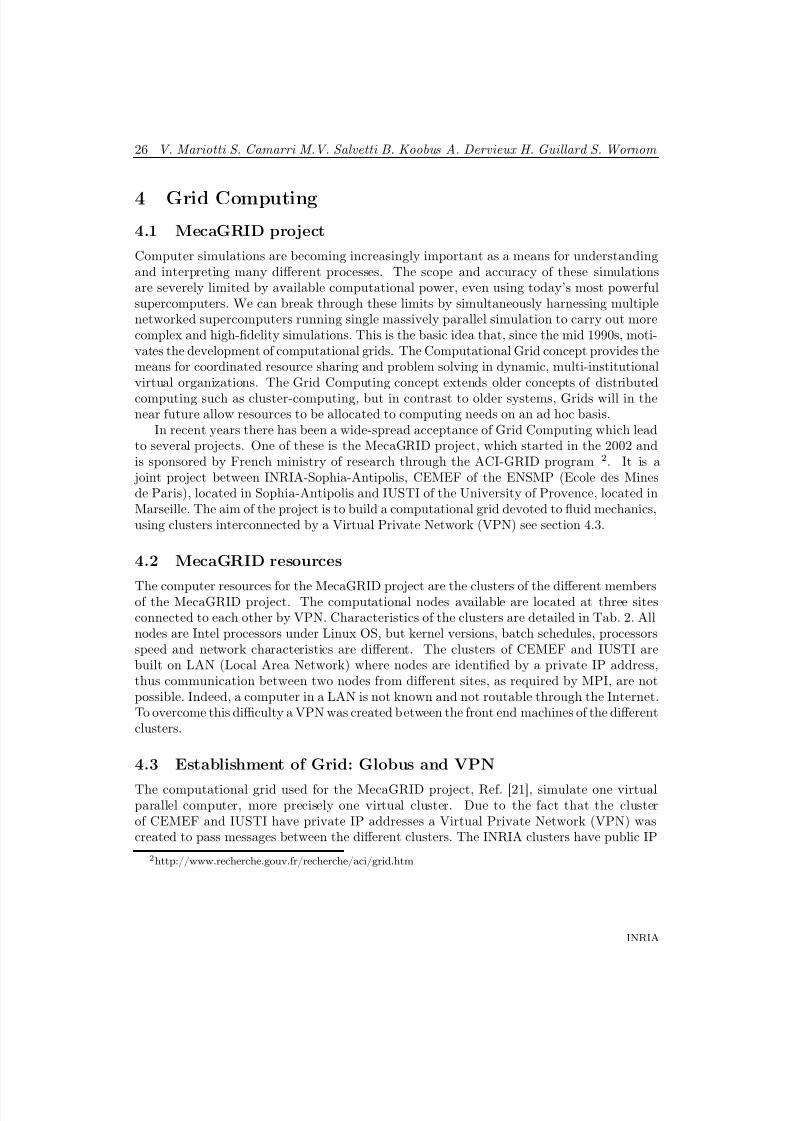
In recent years there has been a wide-spread acceptance of Grid Computing which leadto several projects. One of these is the MecaGRID project, which started in the 2002 andis sponsored by French ministry of research through the ACI-GRID program 2. It is a joint project between INRIA-Sophia-Antipolis, CEMEF of the ENSMP (Ecole des Minesde Paris), located in Sophia-Antipolis and IUSTI of the University of Provence, located inMarseille. The aim of the project is to build a computational grid devoted to fluid mechanics,using clusters interconnected by a Virtual Private Network (VPN) see section 4.3.
4.2 MecaGRID resources
The computer resources for the MecaGRID project are the clusters of the different membersof the MecaGRID project. The computational nodes available are located at three sitesconnected to each other by VPN. Characteristics of the clusters are detailed in Tab. 2. Allnodes are Intel processors under Linux OS, but kernel versions, batch schedules, processorsspeed and network characteristics are different. The clusters of CEMEF and IUSTI arebuilt on LAN (Local Area Network) where nodes are identified by a private IP address,thus communication between two nodes from different sites, as required by MPI, are notpossible. Indeed, a computer in a LAN is not known and not routable through the Internet.To overcome this difficulty a VPN was created between the front end machines of the differentclusters.
4.3 Establishment of Grid: Globus and VPN
The computational grid used for the MecaGRID project, Ref. [21], simulate one virtualparallel computer, more precisely one virtual cluster. Due to the fact that the clusterof CEMEF and IUSTI have private IP addresses a Virtual Private Network (VPN) wascreated to pass messages between the different clusters. The INRIA clusters have public IP
2http://www.recherche.gouv.fr/recherche/aci/grid.htm
INRIA
8/10/2019 CFD Numerical simulation of a jet in crossflow..pdf
http://slidepdf.com/reader/full/cfd-numerical-simulation-of-a-jet-in-crossflowpdf 29/83
Numerical simulation of a jet in crossflow. 27
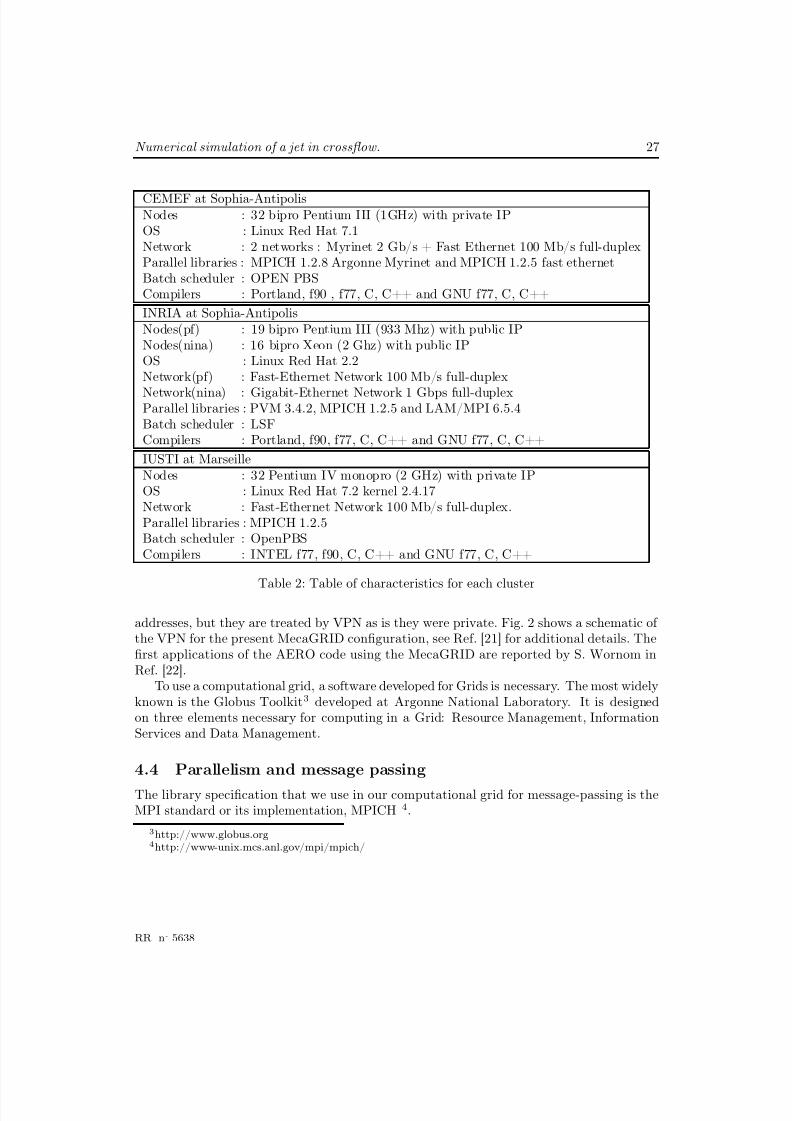
CEMEF at Sophia-AntipolisNodes : 32 bipro Pentium III (1GHz) with private IPOS : Linux Red Hat 7.1Network : 2 networks : Myrinet 2 Gb/s + Fast Ethernet 100 Mb/s full-duplexParallel libraries : MPICH 1.2.8 Argonne Myrinet and MPICH 1.2.5 fast ethernetBatch scheduler : OPEN PBSCompilers : Portland, f90 , f77, C, C++ and GNU f77, C, C++
INRIA at Sophia-AntipolisNodes(pf) : 19 bipro Pentium III (933 Mhz) with public IPNodes(nina) : 16 bipro Xeon (2 Ghz) with public IPOS : Linux Red Hat 2.2Network(pf) : Fast-Ethernet Network 100 Mb/s full-duplex
Network(nina) : Gigabit-Ethernet Network 1 Gbps full-duplexParallel libraries : PVM 3.4.2, MPICH 1.2.5 and LAM/MPI 6.5.4Batch scheduler : LSFCompilers : Portland, f90, f77, C, C++ and GNU f77, C, C++
IUSTI at MarseilleNodes : 32 Pentium IV monopro (2 GHz) with private IPOS : Linux Red Hat 7.2 kernel 2.4.17Network : Fast-Ethernet Network 100 Mb/s full-duplex.Parallel libraries : MPICH 1.2.5Batch scheduler : OpenPBSCompilers : INTEL f77, f90, C, C++ and GNU f77, C, C++
Table 2: Table of characteristics for each cluster
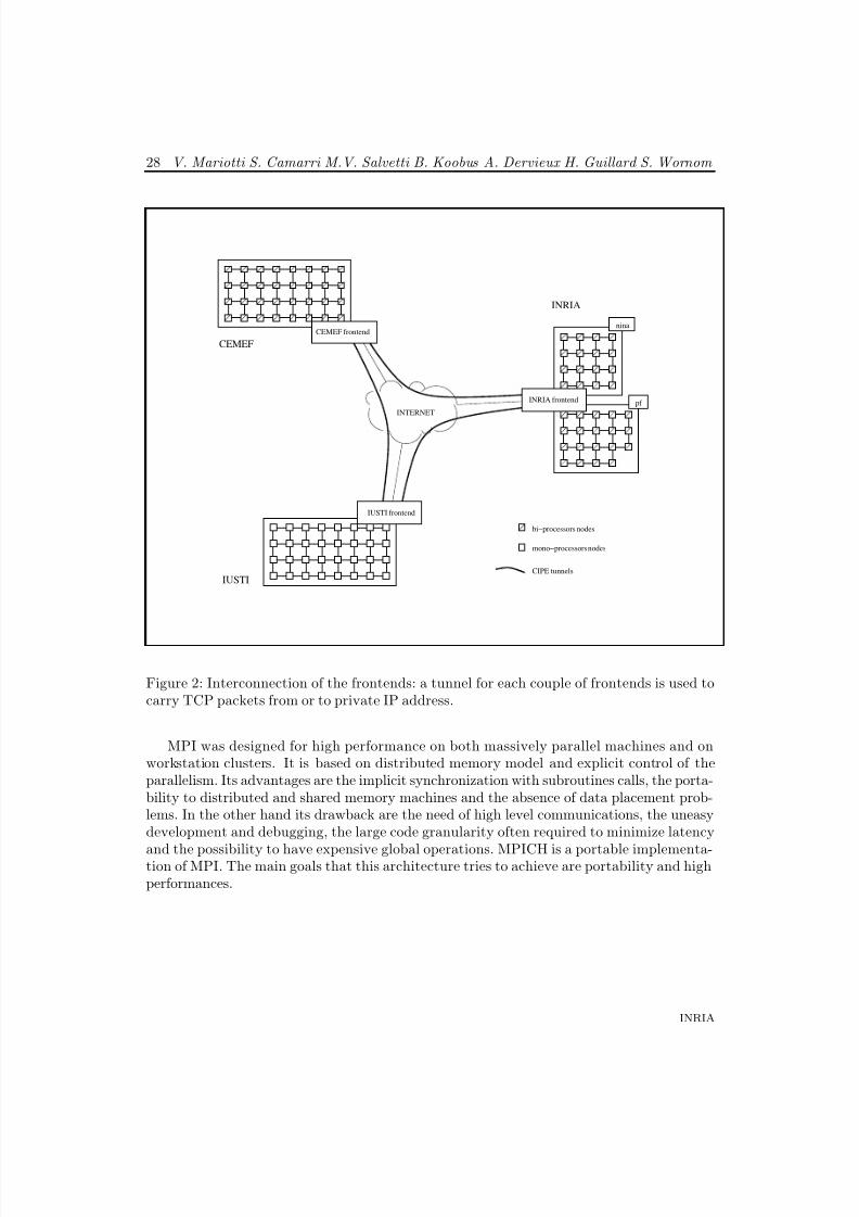
addresses, but they are treated by VPN as is they were private. Fig. 2 shows a schematic of the VPN for the present MecaGRID configuration, see Ref. [21] for additional details. Thefirst applications of the AERO code using the MecaGRID are reported by S. Wornom inRef. [22].
To use a computational grid, a software developed for Grids is necessary. The most widelyknown is the Globus Toolkit3 developed at Argonne National Laboratory. It is designedon three elements necessary for computing in a Grid: Resource Management, InformationServices and Data Management.
4.4 Parallelism and message passing
The library specification that we use in our computational grid for message-passing is theMPI standard or its implementation, MPICH 4.
3http://www.globus.org4http://www-unix.mcs.anl.gov/mpi/mpich/
RR n° 5638
8/10/2019 CFD Numerical simulation of a jet in crossflow..pdf
http://slidepdf.com/reader/full/cfd-numerical-simulation-of-a-jet-in-crossflowpdf 30/83
28 V. Mariotti S. Camarri M.V. Salvetti B. Koobus A. Dervieux H. Guillard S. Wornom
INTERNET
INRIA frontend
CEMEF frontend
IUSTI frontend
nina
pf
bi−processors nodes
mono−processors nodes
IUSTI
CEMEF
CIPE tunnels
INRIA
Figure 2: Interconnection of the frontends: a tunnel for each couple of frontends is used tocarry TCP packets from or to private IP address.
MPI was designed for high performance on both massively parallel machines and onworkstation clusters. It is based on distributed memory model and explicit control of theparallelism. Its advantages are the implicit synchronization with subroutines calls, the porta-bility to distributed and shared memory machines and the absence of data placement prob-lems. In the other hand its drawback are the need of high level communications, the uneasydevelopment and debugging, the large code granularity often required to minimize latency
and the possibility to have expensive global operations. MPICH is a portable implementa-tion of MPI. The main goals that this architecture tries to achieve are portability and highperformances.
INRIA
8/10/2019 CFD Numerical simulation of a jet in crossflow..pdf
http://slidepdf.com/reader/full/cfd-numerical-simulation-of-a-jet-in-crossflowpdf 31/83
Numerical simulation of a jet in crossflow. 29
5 Jet in cross-flow. Flow dynamics and test-case config-uration
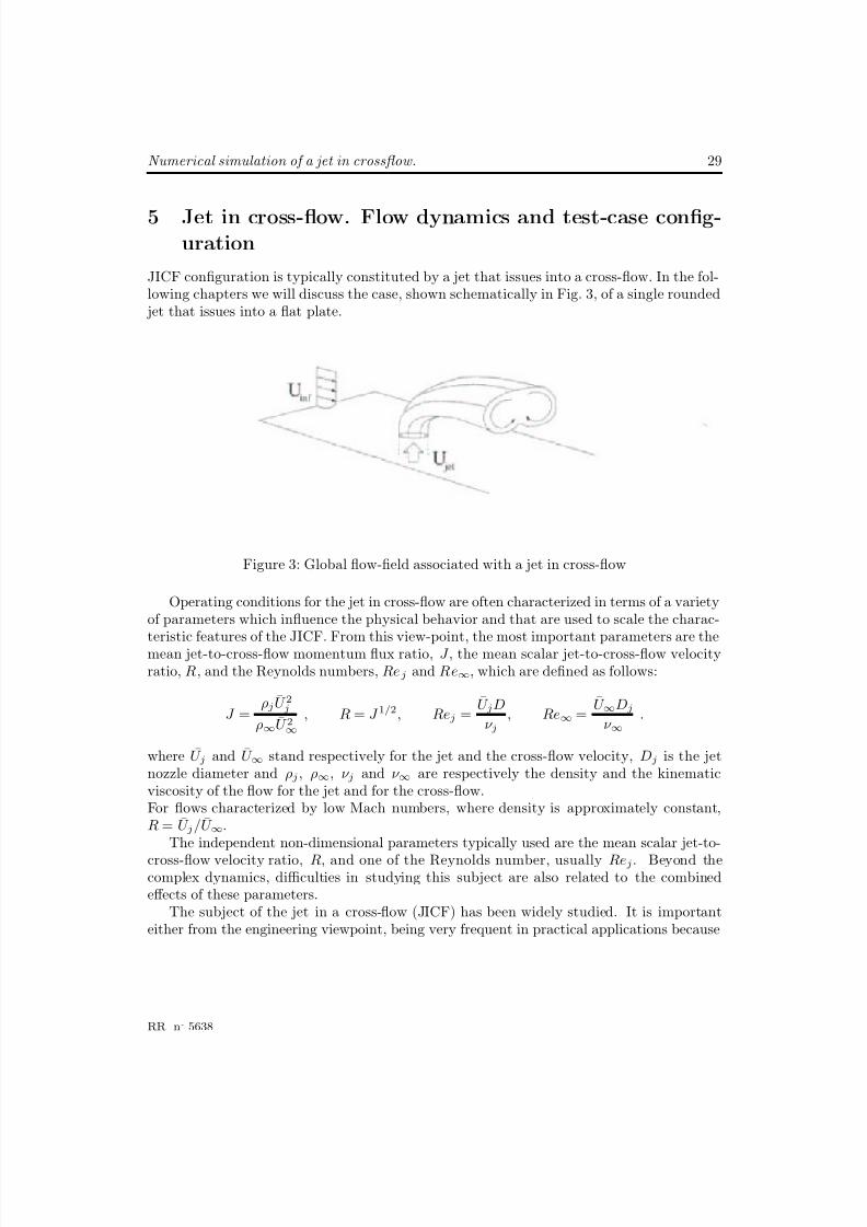
JICF configuration is typically constituted by a jet that issues into a cross-flow. In the fol-lowing chapters we will discuss the case, shown schematically in Fig. 3, of a single rounded jet that issues into a flat plate.
Figure 3: Global flow-field associated with a jet in cross-flow
Operating conditions for the jet in cross-flow are often characterized in terms of a varietyof parameters which influence the physical behavior and that are used to scale the charac-teristic features of the JICF. From this view-point, the most important parameters are themean jet-to-cross-flow momentum flux ratio, J , the mean scalar jet-to-cross-flow velocityratio, R, and the Reynolds numbers, Rej and Re∞, which are defined as follows:
J =ρj
U 2jρ∞ U 2
∞
, R = J 1/2, Rej =U jD
ν j, Re∞ =
U ∞Dj
ν ∞.
where U j and U ∞ stand respectively for the jet and the cross-flow velocity, Dj is the jetnozzle diameter and ρj , ρ∞, ν j and ν ∞ are respectively the density and the kinematicviscosity of the flow for the jet and for the cross-flow.For flows characterized by low Mach numbers, where density is approximately constant,R = U j/U ∞.
The independent non-dimensional parameters typically used are the mean scalar jet-to-
cross-flow velocity ratio, R, and one of the Reynolds number, usually Rej. Beyond thecomplex dynamics, difficulties in studying this subject are also related to the combinedeffects of these parameters.
The subject of the jet in a cross-flow (JICF) has been widely studied. It is importanteither from the engineering viewpoint, being very frequent in practical applications because
RR n° 5638
8/10/2019 CFD Numerical simulation of a jet in crossflow..pdf
http://slidepdf.com/reader/full/cfd-numerical-simulation-of-a-jet-in-crossflowpdf 32/83
30 V. Mariotti S. Camarri M.V. Salvetti B. Koobus A. Dervieux H. Guillard S. Wornom
of its ability to mix rapidly with cross-flow and to introduce a controlled jet force into flow-field (e.g. injectors for cooling systems, jets for V-STOL aircraft, exhaust of vehicles) or forbasic research, because of the variety of fluid dynamic phenomena involved. Investigations onthe JICF have started in the 1930s, Ref.[28]. Since, there have been numerous investigationson the JICF leading to the perception that the JICF, in contrast to other flows like jets andmixing layers, cannot be described in terms of self similarity and Reynolds dependence, dueto the strong nonlinear effects. The systematic analysis of the JICF started in 1970s with thediscovery and acceptance of coherent structures that are able to explain various nonlineareffects in the JICF.
5.1 Vortex system associated with the transverse jet
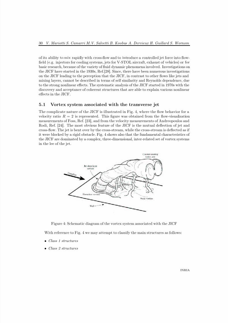
The complicate nature of the JICF is illustrated in Fig. 4, where the flow behavior for avelocity ratio R = 2 is represented. This figure was obtained from the flow-visualizationmeasurements of Foss, Ref. [23], and from the velocity measurements of Andreopoulos andRodi, Ref. [24]. The most obvious feature of the JICF is the mutual deflection of jet andcross-flow. The jet is bent over by the cross-stream, while the cross-stream is deflected as if it were blocked by a rigid obstacle. Fig. 4 shows also that the fundamental characteristics of the JICF are dominated by a complex, three-dimensional, inter-related set of vortex systemsin the lee of the jet.
Figure 4: Schematic diagram of the vortex system associated with the JICF
With reference to Fig. 4 we may attempt to classify the main structures as follows:
• Class 1 structures
• Class 2 structures
INRIA
8/10/2019 CFD Numerical simulation of a jet in crossflow..pdf
http://slidepdf.com/reader/full/cfd-numerical-simulation-of-a-jet-in-crossflowpdf 33/83
Numerical simulation of a jet in crossflow. 31
5.1.1 Class 1 structures
The class 1 structures are originated by the interaction of the jet with the cross-flow and thewall and cannot be recognized in free jets. Among structures of this kind we may includethe following vortex systems, Ref. [24] and Ref. [25]:
• Counter-Rotating Vortex Pair (CRVP)
• Horseshoe Vortices (HSV)
• Upright vortices (UV)
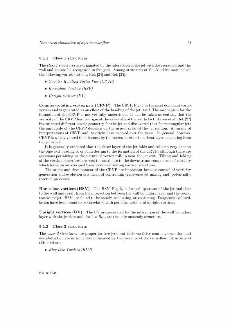
Counter-rotating vortex pair (CRVP) The CRVP, Fig. 5, is the most dominant vortexsystem and is generated as an effect of the bending of the jet itself. The mechanism for the
formation of the CRVP is not yet fully understood. It can be taken as certain, that thevorticity of the CRVP has its origin at the side-walls of the jet. In fact, Haven et al. Ref. [27]investigated different nozzle geometry for the jet and discovered that for rectangular jetsthe amplitude of the CRVP depends on the aspect ratio of the jet section. A variety of interpretations of CRVP and its origin have evolved over the years. In general, however,CRVP is widely viewed to be formed by the vortex sheet or thin shear layer emanating fromthe jet nozzle.
It is generally accepted that the shear layer of the jet folds and rolls up very near tothe pipe exit, leading to or contributing to the formation of the CRVP, although there arequestions pertaining to the nature of vortex roll-up near the jet exit. Tilting and foldingof the vortical structures are seen to contribute to the downstream components of vorticitywhich form, on an averaged basis, counter-rotating vortical structures.
The origin and development of the CRVP are important because control of vorticitygeneration and evolution is a mean of controlling transverse jet mixing and, potentially,reaction processes.
Horseshoe vortices (HSV) The HSV, Fig. 6, is formed upstream of the jet and closeto the wall and result from the interaction between the wall boundary layer and the roundtransverse jet. HSV are found to be steady, oscillating, or coalescing. Frequencies of oscil-lation have been found to be correlated with periodic motions of upright vortices.
Upright vortices (UV) The UV are generated by the interaction of the wall boundarylayer with the jet flow and, for low Rej, are the only unsteady structure.
5.1.2 Class 2 structuresThe class 2 structures are proper for free jets, but their vorticity content, evolution anddestabilization are in some way influenced by the presence of the cross-flow. Structures of this kind are:
• Ring-Like Vortices (RLV)
RR n° 5638
8/10/2019 CFD Numerical simulation of a jet in crossflow..pdf
http://slidepdf.com/reader/full/cfd-numerical-simulation-of-a-jet-in-crossflowpdf 34/83
32 V. Mariotti S. Camarri M.V. Salvetti B. Koobus A. Dervieux H. Guillard S. Wornom
Figure 5: Counter-rotating vortex pair
Ring-like vortices The RLV are formed from the shear layer of the jet flow and theirshape and spatial evolution is distorted by the presence of the cross-stream. With the CRVP,they determine the dominant features of the velocity and vorticity fields and their dynamicsis of great interest from the practical viewpoint since they are mainly responsible for mixingand for mass, momentum and heat transfer.
5.2 Flow configuration
The flow configuration used in our simulations is that of a jet which forms from as a pipeflow and then issues into a flat-plate boundary layer through an orifice in the plane of theflat plate.
The velocity ratio, R, is a very important parameter for this configuration, indeed, theflow regime can change depending on R. If R < 0.5 the jet flow is weaker than the cross-flow,so it is not able to break through the wall boundary layer of the cross-flow and plays the roleof an obstacle for the cross-flow. In this case the far field is primarily governed by the crossflow. This flow configuration is important for turbine blade coolings. If 1 < R < 10 the jetis able to push through the boundary layer, which plays a smaller role. These velocity ratioare common for combustion applications. The velocity ratios higher then 10 have differentfeatures as they behave more and more like free jets with increasing velocity ratio.
In our simulations we have used a velocity ratio of 2. The considered Reynolds number,based on the pipe diameter and on the jet velocity, U j , is:
Re = L U j
ν = 82000, (55)
and the Mach number of the undisturbed flow, M, is assumed to be equal to 0.1.
INRIA
8/10/2019 CFD Numerical simulation of a jet in crossflow..pdf
http://slidepdf.com/reader/full/cfd-numerical-simulation-of-a-jet-in-crossflowpdf 35/83
Numerical simulation of a jet in crossflow. 33
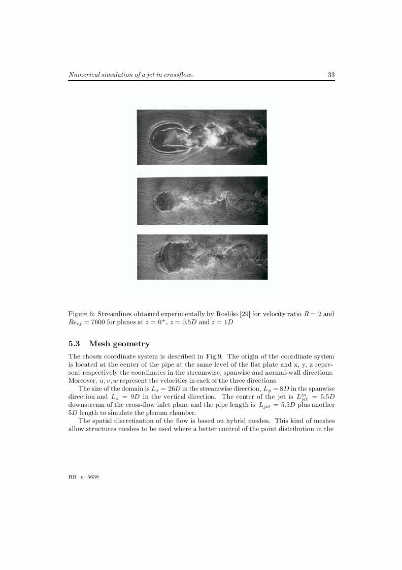
Figure 6: Streamlines obtained experimentally by Roshko [29] for velocity ratio R = 2 andRecf = 7600 for planes at z = 0+, z = 0.5D and z = 1D
5.3 Mesh geometry
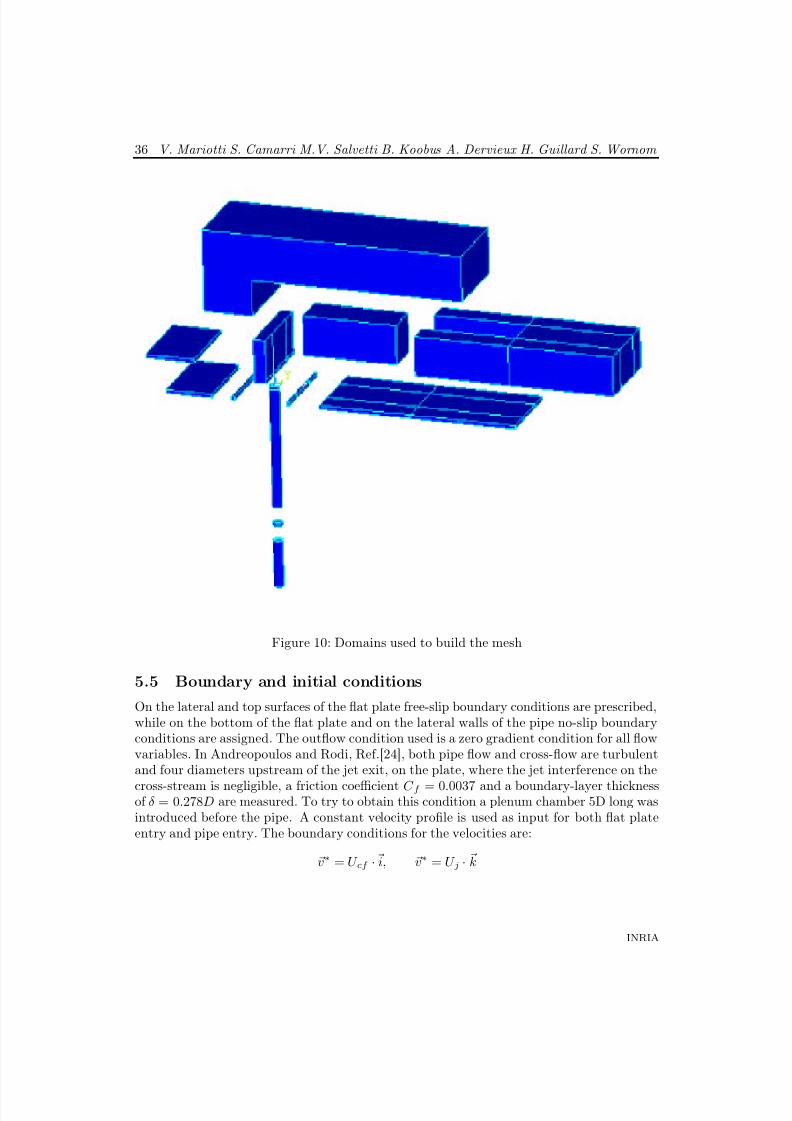
The chosen coordinate system is described in Fig.9. The origin of the coordinate systemis located at the center of the pipe at the same level of the flat plate and x, y, z repre-sent respectively the coordinates in the streamwise, spanwise and normal-wall directions.Moreover, u, v,w represent the velocities in each of the three directions.
The size of the domain is Lx = 26D in the streamwise direction, Ly = 8D in the spanwise
direction and Lz = 9D in the vertical direction. The center of the jet is Lin
jet = 5.5Ddownstream of the cross-flow inlet plane and the pipe length is Ljet = 5.5D plus another5D length to simulate the plenum chamber.
The spatial discretization of the flow is based on hybrid meshes. This kind of meshesallow structures meshes to be used where a better control of the point distribution in the
RR n° 5638
8/10/2019 CFD Numerical simulation of a jet in crossflow..pdf
http://slidepdf.com/reader/full/cfd-numerical-simulation-of-a-jet-in-crossflowpdf 36/83
34 V. Mariotti S. Camarri M.V. Salvetti B. Koobus A. Dervieux H. Guillard S. Wornom
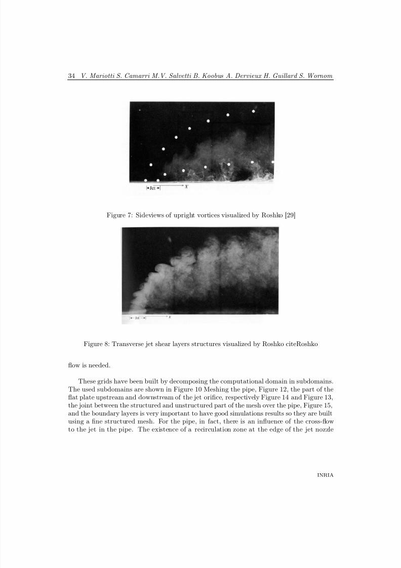
Figure 7: Sideviews of upright vortices visualized by Roshko [29]
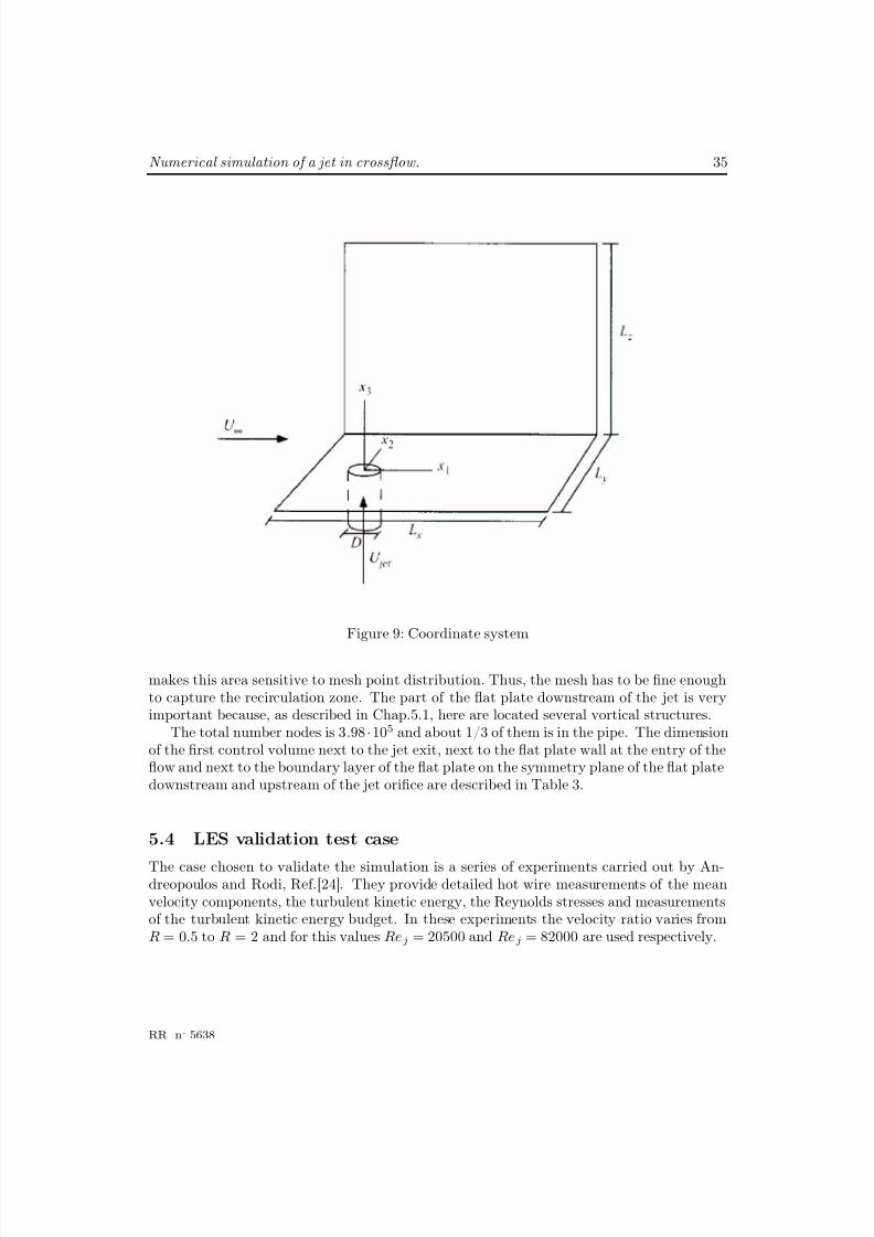
Figure 8: Transverse jet shear layers structures visualized by Roshko citeRoshko
flow is needed.
These grids have been built by decomposing the computational domain in subdomains.The used subdomains are shown in Figure 10 Meshing the pipe, Figure 12, the part of the
flat plate upstream and downstream of the jet orifice, respectively Figure 14 and Figure 13,the joint between the structured and unstructured part of the mesh over the pipe, Figure 15,and the boundary layers is very important to have good simulations results so they are builtusing a fine structured mesh. For the pipe, in fact, there is an influence of the cross-flowto the jet in the pipe. The existence of a recirculation zone at the edge of the jet nozzle
INRIA
8/10/2019 CFD Numerical simulation of a jet in crossflow..pdf
http://slidepdf.com/reader/full/cfd-numerical-simulation-of-a-jet-in-crossflowpdf 37/83
Numerical simulation of a jet in crossflow. 35
Figure 9: Coordinate system
makes this area sensitive to mesh point distribution. Thus, the mesh has to be fine enoughto capture the recirculation zone. The part of the flat plate downstream of the jet is veryimportant because, as described in Chap.5.1, here are located several vortical structures.
The total number nodes is 3.98 ·105 and about 1/3 of them is in the pipe. The dimensionof the first control volume next to the jet exit, next to the flat plate wall at the entry of theflow and next to the boundary layer of the flat plate on the symmetry plane of the flat platedownstream and upstream of the jet orifice are described in Table 3.
5.4 LES validation test case
The case chosen to validate the simulation is a series of experiments carried out by An-dreopoulos and Rodi, Ref.[24]. They provide detailed hot wire measurements of the meanvelocity components, the turbulent kinetic energy, the Reynolds stresses and measurementsof the turbulent kinetic energy budget. In these experiments the velocity ratio varies fromR = 0.5 to R = 2 and for this values Rej = 20500 and Rej = 82000 are used respectively.
RR n° 5638
8/10/2019 CFD Numerical simulation of a jet in crossflow..pdf
http://slidepdf.com/reader/full/cfd-numerical-simulation-of-a-jet-in-crossflowpdf 38/83
36 V. Mariotti S. Camarri M.V. Salvetti B. Koobus A. Dervieux H. Guillard S. Wornom
Figure 10: Domains used to build the mesh
5.5 Boundary and initial conditions
On the lateral and top surfaces of the flat plate free-slip boundary conditions are prescribed,while on the bottom of the flat plate and on the lateral walls of the pipe no-slip boundaryconditions are assigned. The outflow condition used is a zero gradient condition for all flowvariables. In Andreopoulos and Rodi, Ref.[24], both pipe flow and cross-flow are turbulentand four diameters upstream of the jet exit, on the plate, where the jet interference on the
cross-stream is negligible, a friction coefficient C f = 0.0037 and a boundary-layer thicknessof δ = 0.278D are measured. To try to obtain this condition a plenum chamber 5D long wasintroduced before the pipe. A constant velocity profile is used as input for both flat plateentry and pipe entry. The boundary conditions for the velocities are:
v∗ = U cf · i, v∗ = U j · k
INRIA
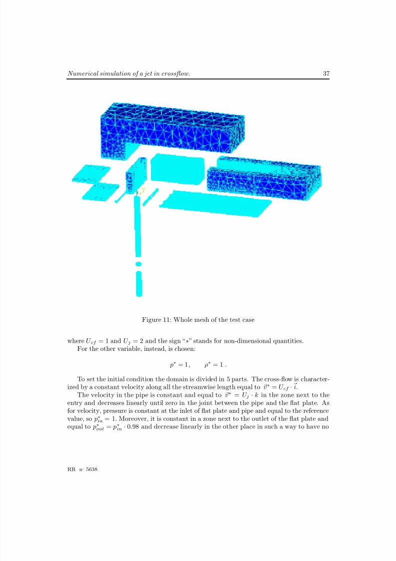
8/10/2019 CFD Numerical simulation of a jet in crossflow..pdf
http://slidepdf.com/reader/full/cfd-numerical-simulation-of-a-jet-in-crossflowpdf 39/83
Numerical simulation of a jet in crossflow. 37
Figure 11: Whole mesh of the test case
where U cf = 1 and U j = 2 and the sign “∗” stands for non-dimensional quantities.For the other variable, instead, is chosen:
p∗ = 1, ρ∗ = 1 .
To set the initial condition the domain is divided in 5 parts. The cross-flow is character-ized by a constant velocity along all the streamwise length equal to v∗ = U cf · i.
The velocity in the pipe is constant and equal to v∗ = U j · k in the zone next to theentry and decreases linearly until zero in the joint between the pipe and the flat plate. Asfor velocity, pressure is constant at the inlet of flat plate and pipe and equal to the referencevalue, so p∗in = 1. Moreover, it is constant in a zone next to the outlet of the flat plate andequal to p∗out = p∗in · 0.98 and decrease linearly in the other place in such a way to have no
RR n° 5638
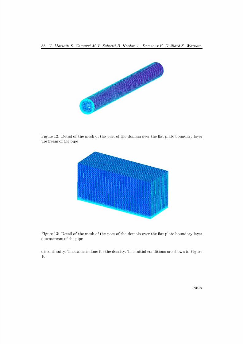
8/10/2019 CFD Numerical simulation of a jet in crossflow..pdf
http://slidepdf.com/reader/full/cfd-numerical-simulation-of-a-jet-in-crossflowpdf 40/83
38 V. Mariotti S. Camarri M.V. Salvetti B. Koobus A. Dervieux H. Guillard S. Wornom
Figure 12: Detail of the mesh of the part of the domain over the flat plate boundary layerupstream of the pipe
Figure 13: Detail of the mesh of the part of the domain over the flat plate boundary layerdownstream of the pipe
discontinuity. The same is done for the density. The initial conditions are shown in Figure16.
INRIA
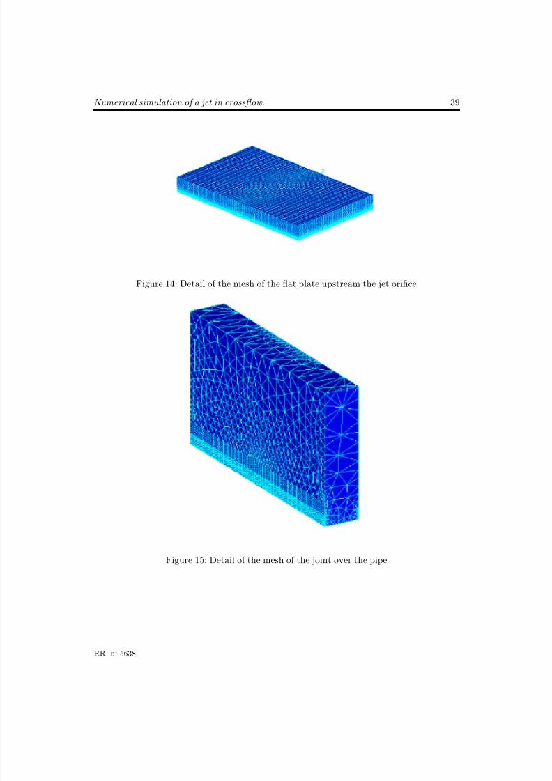
8/10/2019 CFD Numerical simulation of a jet in crossflow..pdf
http://slidepdf.com/reader/full/cfd-numerical-simulation-of-a-jet-in-crossflowpdf 41/83
Numerical simulation of a jet in crossflow. 39
Figure 14: Detail of the mesh of the flat plate upstream the jet orifice
Figure 15: Detail of the mesh of the joint over the pipe
RR n° 5638
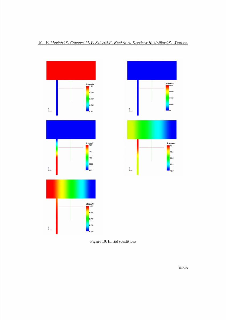
8/10/2019 CFD Numerical simulation of a jet in crossflow..pdf
http://slidepdf.com/reader/full/cfd-numerical-simulation-of-a-jet-in-crossflowpdf 42/83
40 V. Mariotti S. Camarri M.V. Salvetti B. Koobus A. Dervieux H. Guillard S. Wornom
Figure 16: Initial conditions
INRIA
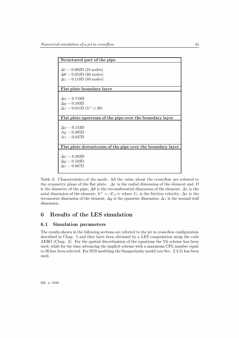
8/10/2019 CFD Numerical simulation of a jet in crossflow..pdf
http://slidepdf.com/reader/full/cfd-numerical-simulation-of-a-jet-in-crossflowpdf 43/83
Numerical simulation of a jet in crossflow. 41
Structured part of the pipe
∆r = 0.002D (24 nodes)∆θ = 0.052D (60 nodes)∆z = 0.118D (68 nodes)
Flat plate boundary layer
∆x = 0.719D∆y = 0.103D∆z = 0.011D (h+ 30)
Flat plate upstream of the pipe over the boundary layer
∆x = 0.153D∆y = 0.385D∆z = 0.047D
Flat plate downstream of the pipe over the boundary layer
∆x = 0.202D∆y = 0.103D∆z = 0.067D
Table 3: Characteristics of the mesh: All the value about the cross-flow are referred tothe symmetry plane of the flat plate. ∆r is the radial dimension of the element and Dis the diameter of the pipe; ∆θ is the circumferential dimension of the element; ∆z is theaxial dimension of the element; h+ = zU τ /ν where U τ is the friction velocity; ∆x is thestreamwise dimension of the element; ∆y is the spanwise dimension; ∆z is the normal-walldimension.
6 Results of the LES simulation
6.1 Simulation parameters
The results shown in the following sections are referred to the jet in cross-flow configuration
described in Chap. 5 and they have been obtained by a LES computation using the codeAERO (Chap. 3). For the spatial discretization of the equations the V6 scheme has beenused, while for the time advancing the implicit scheme with a maximum CFL number equalto 20 has been selected. For SGS modeling the Smagorinsky model (see Sec. 2.3.3) has beenused.
RR n° 5638
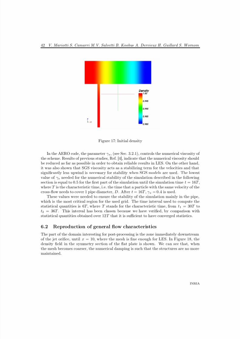
8/10/2019 CFD Numerical simulation of a jet in crossflow..pdf
http://slidepdf.com/reader/full/cfd-numerical-simulation-of-a-jet-in-crossflowpdf 44/83
42 V. Mariotti S. Camarri M.V. Salvetti B. Koobus A. Dervieux H. Guillard S. Wornom
Figure 17: Initial density
In the AERO code, the parameter γ s, (see Sec. 3.2.1), controls the numerical viscosity of the scheme. Results of previous studies, Ref. [4], indicate that the numerical viscosity shouldbe reduced as far as possible in order to obtain reliable results in LES. On the other hand,it was also shown that SGS viscosity acts as a stabilizing term for the velocities and thatsignificantly less upwind is necessary for stability when SGS models are used. The lowest
value of γ s needed for the numerical stability of the simulation described in the followingsection is equal to 0.5 for the first part of the simulation until the simulation time t = 16T ,where T is the characteristic time, i.e. the time that a particle with the same velocity of thecross-flow needs to cover 1 pipe diameter, D . After t = 16T , γ s = 0.4 is used.
These values were needed to ensure the stability of the simulation mainly in the pipe,which is the most critical region for the used grid. The time interval used to compute thestatistical quantities is 6T , where T stands for the characteristic time, from t1 = 30T tot2 = 36T . This interval has been chosen because we have verified, by comparison withstatistical quantities obtained over 12T that it is sufficient to have converged statistics.
6.2 Reproduction of general flow characteristics
The part of the domain interesting for post-processing is the zone immediately downstream
of the jet orifice, until x = 10, where the mesh is fine enough for LES. In Figure 18, thedensity field in the symmetry section of the flat plate is shown. We can see that, whenthe mesh becomes coarser, the numerical damping is such that the structures are no moremaintained.
INRIA
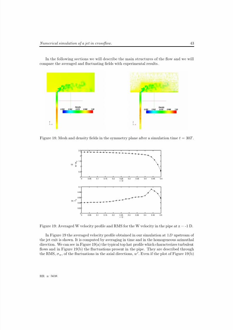
8/10/2019 CFD Numerical simulation of a jet in crossflow..pdf
http://slidepdf.com/reader/full/cfd-numerical-simulation-of-a-jet-in-crossflowpdf 45/83
Numerical simulation of a jet in crossflow. 43
In the following sections we will describe the main structures of the flow and we willcompare the averaged and fluctuating fields with experimental results.
Figure 18: Mesh and density fields in the symmetry plane after a simulation time t = 30T .
0 0.05 0.1 0.15 0.2 0.25 0.3 0.35 0.4 0.45 0.50
0.5
1
1.5
2
2.5
r / D
W /
W c
f
0 0.05 0.1 0.15 0.2 0.25 0.3 0.35 0.4 0.45 0.50
0.02
0.04
0.06
0.08
0.1
σ w
r / D
(a)
(b)
Figure 19: Averaged W velocity profile and RMS for the W velocity in the pipe at z = -1 D.
In Figure 19 the averaged velocity profile obtained in our simulation at 1D upstream of the jet exit is shown. It is computed by averaging in time and in the homogeneous azimuthaldirection. We can see in Figure 19(a) the typical top hat profile which characterizes turbulentflows and in Figure 19(b) the fluctuations present in the pipe. They are described throughthe RMS, σw, of the fluctuations in the axial directions, w . Even if the plot of Figure 19(b)
RR n° 5638
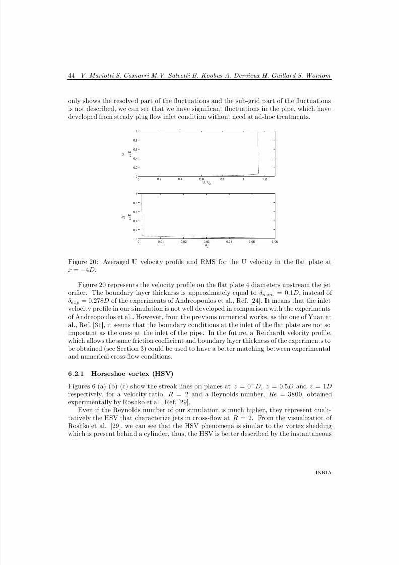
8/10/2019 CFD Numerical simulation of a jet in crossflow..pdf
http://slidepdf.com/reader/full/cfd-numerical-simulation-of-a-jet-in-crossflowpdf 46/83
44 V. Mariotti S. Camarri M.V. Salvetti B. Koobus A. Dervieux H. Guillard S. Wornom
only shows the resolved part of the fluctuations and the sub-grid part of the fluctuationsis not described, we can see that we have significant fluctuations in the pipe, which havedeveloped from steady plug flow inlet condition without need at ad-hoc treatments.
0 0.2 0.4 0.6 0.8 1 1.20
0.2
0.4
0.6
0.8
1
U / Ucf
z / D
0 0.01 0.02 0.03 0.04 0.05 0.060
0.2
0.4
0.6
0.8
1
σu
z / D
(a)
(b)
Figure 20: Averaged U velocity profile and RMS for the U velocity in the flat plate atx = −4D.
Figure 20 represents the velocity profile on the flat plate 4 diameters upstream the jetorifice. The boundary layer thickness is approximately equal to δ num = 0.1D, instead of δ exp = 0.278D of the experiments of Andreopoulos et al., Ref. [24]. It means that the inletvelocity profile in our simulation is not well developed in comparison with the experimentsof Andreopoulos et al.. However, from the previous numerical works, as the one of Yuan atal., Ref. [31], it seems that the boundary conditions at the inlet of the flat plate are not soimportant as the ones at the inlet of the pipe. In the future, a Reichardt velocity profile,which allows the same friction coefficient and boundary layer thickness of the experiments tobe obtained (see Section 3) could be used to have a better matching between experimentaland numerical cross-flow conditions.
6.2.1 Horseshoe vortex (HSV)
Figures 6 (a)-(b)-(c) show the streak lines on planes at z = 0+D, z = 0.5D and z = 1D
respectively, for a velocity ratio, R = 2 and a Reynolds number, Re = 3800, obtainedexperimentally by Roshko et al., Ref. [29].Even if the Reynolds number of our simulation is much higher, they represent quali-
tatively the HSV that characterize jets in cross-flow at R = 2. From the visualization of Roshko et al. [29], we can see that the HSV phenomena is similar to the vortex sheddingwhich is present behind a cylinder, thus, the HSV is better described by the instantaneous
INRIA
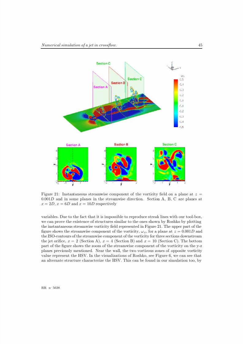
8/10/2019 CFD Numerical simulation of a jet in crossflow..pdf
http://slidepdf.com/reader/full/cfd-numerical-simulation-of-a-jet-in-crossflowpdf 47/83
Numerical simulation of a jet in crossflow. 45
Figure 21: Instantaneous streamwise component of the vorticity field on a plane at z =0.001D and in some planes in the streamwise direction. Section A, B, C are planes atx = 2D, x = 6D and x = 10D respectively
variables. Due to the fact that it is impossible to reproduce streak lines with our tool-box,we can prove the existence of structures similar to the ones shown by Roshko by plottingthe instantaneous streamwise vorticity field represented in Figure 21. The upper part of thefigure shows the streamwise component of the vorticity, ωx, for a plane at z = 0.001D andthe ISO-contours of the streamwise component of the vorticity for three sections downstream
the jet orifice, x = 2 (Section A), x = 4 (Section B) and x = 10 (Section C). The bottompart of the figure shows the zoom of the streamwise component of the vorticity on the y-zplanes previously mentioned. Near the wall, the two vorticous zones of opposite vorticityvalue represent the HSV. In the visualizations of Roshko, see Figure 6, we can see thatan alternate structure characterize the HSV. This can be found in our simulation too, by
RR n° 5638
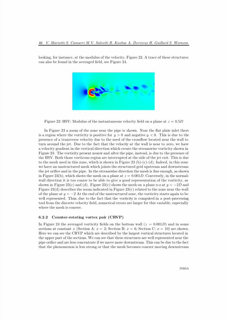
8/10/2019 CFD Numerical simulation of a jet in crossflow..pdf
http://slidepdf.com/reader/full/cfd-numerical-simulation-of-a-jet-in-crossflowpdf 48/83
46 V. Mariotti S. Camarri M.V. Salvetti B. Koobus A. Dervieux H. Guillard S. Wornom
looking, for instance, at the modulus of the velocity, Figure 22. A trace of these structurescan also be found in the averaged field, see Figure 24.
Figure 22: HSV: Modulus of the instantaneous velocity field on a plane at z = 0.5D
In Figure 23 a zoom of the zone near the pipe is shown. Near the flat plate inlet thereis a region where the vorticity is positive for y > 0 and negative y < 0. This is due to thepresence of a transverse velocity due to the need of the crossflow located near the wall toturn around the jet. Due to the fact that the velocity at the wall is near to zero, we havea velocity gradient in the vertical direction which create the streamwise vorticity shown inFigure 23. The vorticity present nearer and after the pipe, instead, is due to the presence of the HSV. Both those vorticous region are interrupted at the side of the jet exit. This is dueto the mesh used in this zone, which is shown in Figure 23 (b)-(c)-(d). Indeed, in this zone
we have an unstructured mesh which joints the structured grid upstream and downstreamthe jet orifice and in the pipe. In the streamwise direction the mesh is fine enough, as shownin Figure 23(b), which shows the mesh on a plane at z = 0.001D. Conversely, in the normal-wall direction it is too coarse to be able to give a good representation of the vorticity, asshown in Figure 23(c) and (d). Figure 23(c) shows the mesh on a plane x-z at y = −2D andFigure 23(d) describes the zoom indicated in Figure 23(c) related to the zone near the wallof the plane at y = −2 At the end of the unstructured zone, the vorticity starts again to bewell represented. Thus, due to the fact that the vorticity is computed in a post-processingtool from the discrete velocity field, numerical errors are larger for this variable, especiallywhere the mesh is coarser.
6.2.2 Counter-rotating vortex pair (CRVP)
In Figure 24 the averaged vorticity fields on the bottom wall (z = 0.001D) and in somesections at constant x (Section A: x = 2; Section B: x = 6; Section C: x = 10) are shown.Here we can see the CRVP which are described by the largest vortical structures located inthe upper part of the sections. We can see that these structures are well represented near thepipe orifice and are less concentrate if we move more downstream. This can be due to the factthat the phenomenon is less strong or that the mesh becomes coarser moving downstream
INRIA
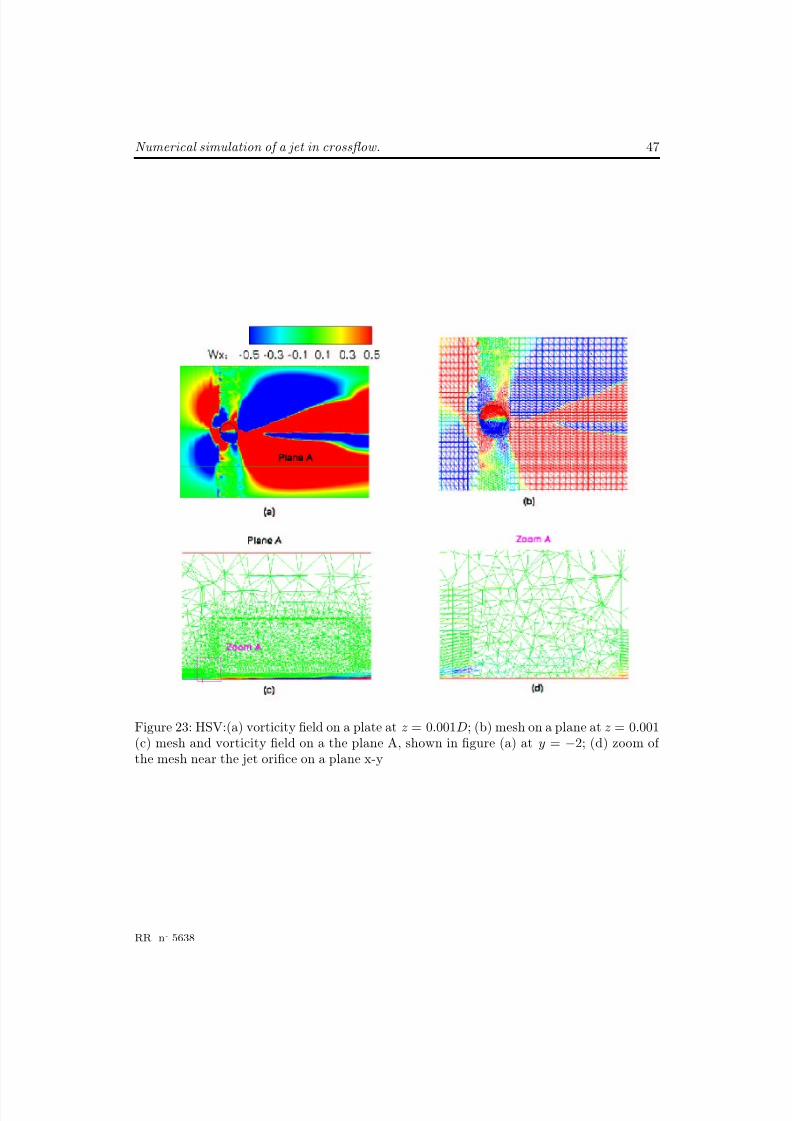
8/10/2019 CFD Numerical simulation of a jet in crossflow..pdf
http://slidepdf.com/reader/full/cfd-numerical-simulation-of-a-jet-in-crossflowpdf 49/83
Numerical simulation of a jet in crossflow. 47
Figure 23: HSV:(a) vorticity field on a plate at z = 0.001D; (b) mesh on a plane at z = 0.001(c) mesh and vorticity field on a the plane A, shown in figure (a) at y = −2; (d) zoom of the mesh near the jet orifice on a plane x-y
RR n° 5638
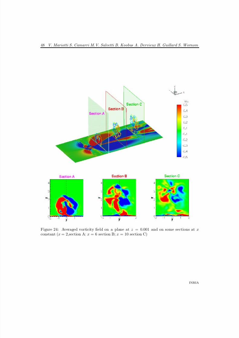
8/10/2019 CFD Numerical simulation of a jet in crossflow..pdf
http://slidepdf.com/reader/full/cfd-numerical-simulation-of-a-jet-in-crossflowpdf 50/83
48 V. Mariotti S. Camarri M.V. Salvetti B. Koobus A. Dervieux H. Guillard S. Wornom
Figure 24: Averaged vorticity field on a plane at z = 0.001 and on some sections at xconstant (x = 2,section A; x = 6 section B; x = 10 section C)
INRIA
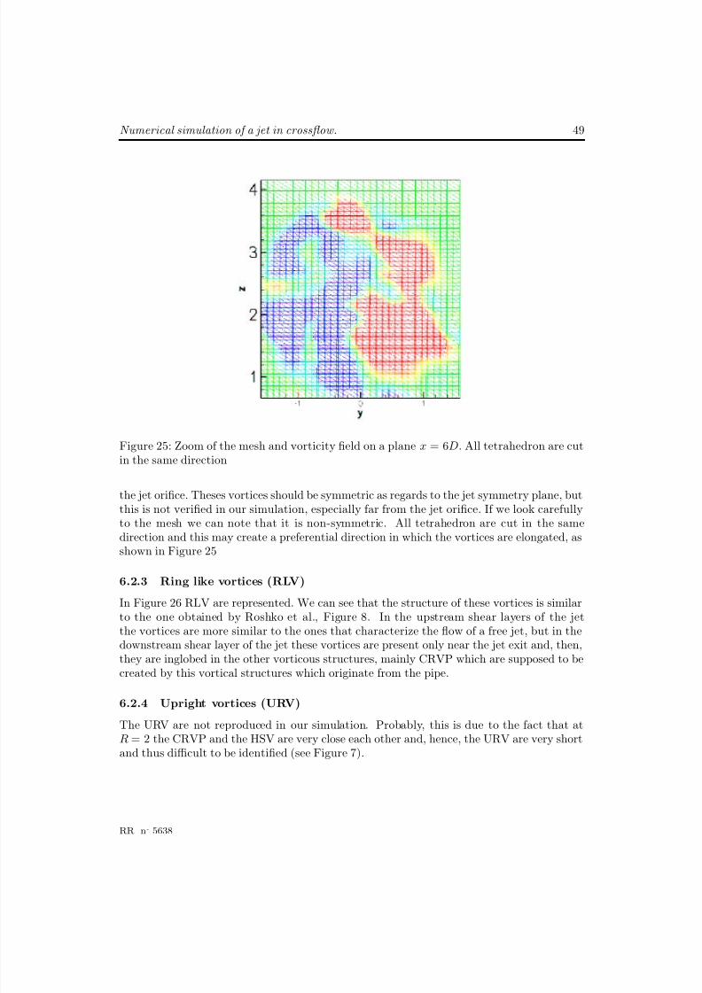
8/10/2019 CFD Numerical simulation of a jet in crossflow..pdf
http://slidepdf.com/reader/full/cfd-numerical-simulation-of-a-jet-in-crossflowpdf 51/83
Numerical simulation of a jet in crossflow. 49
Figure 25: Zoom of the mesh and vorticity field on a plane x = 6D. All tetrahedron are cutin the same direction
the jet orifice. Theses vortices should be symmetric as regards to the jet symmetry plane, butthis is not verified in our simulation, especially far from the jet orifice. If we look carefully
to the mesh we can note that it is non-symmetric. All tetrahedron are cut in the samedirection and this may create a preferential direction in which the vortices are elongated, asshown in Figure 25
6.2.3 Ring like vortices (RLV)
In Figure 26 RLV are represented. We can see that the structure of these vortices is similarto the one obtained by Roshko et al., Figure 8. In the upstream shear layers of the jetthe vortices are more similar to the ones that characterize the flow of a free jet, but in thedownstream shear layer of the jet these vortices are present only near the jet exit and, then,they are inglobed in the other vorticous structures, mainly CRVP which are supposed to becreated by this vortical structures which originate from the pipe.
6.2.4 Upright vortices (URV)
The URV are not reproduced in our simulation. Probably, this is due to the fact that atR = 2 the CRVP and the HSV are very close each other and, hence, the URV are very shortand thus difficult to be identified (see Figure 7).
RR n° 5638
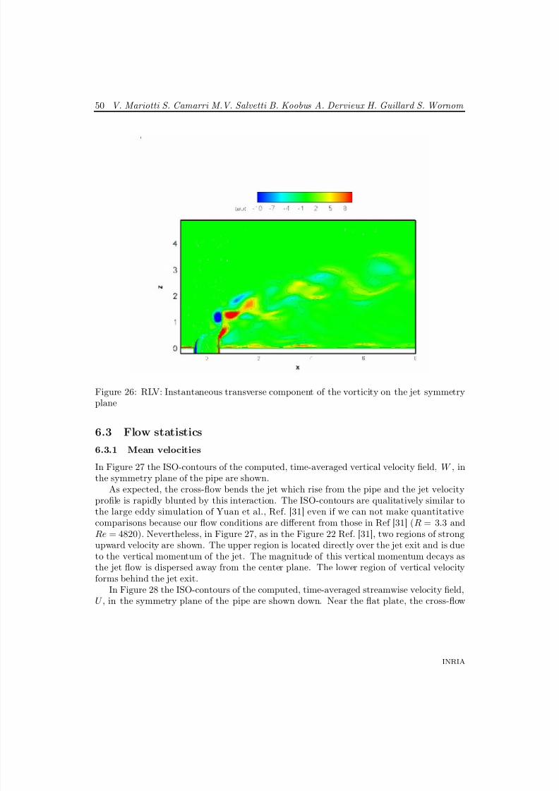
8/10/2019 CFD Numerical simulation of a jet in crossflow..pdf
http://slidepdf.com/reader/full/cfd-numerical-simulation-of-a-jet-in-crossflowpdf 52/83
50 V. Mariotti S. Camarri M.V. Salvetti B. Koobus A. Dervieux H. Guillard S. Wornom
Figure 26: RLV: Instantaneous transverse component of the vorticity on the jet symmetryplane
6.3 Flow statistics
6.3.1 Mean velocities
In Figure 27 the ISO-contours of the computed, time-averaged vertical velocity field, W , inthe symmetry plane of the pipe are shown.
As expected, the cross-flow bends the jet which rise from the pipe and the jet velocityprofile is rapidly blunted by this interaction. The ISO-contours are qualitatively similar tothe large eddy simulation of Yuan et al., Ref. [31] even if we can not make quantitativecomparisons because our flow conditions are different from those in Ref [31] (R = 3.3 andRe = 4820). Nevertheless, in Figure 27, as in the Figure 22 Ref. [31], two regions of strongupward velocity are shown. The upper region is located directly over the jet exit and is due
to the vertical momentum of the jet. The magnitude of this vertical momentum decays asthe jet flow is dispersed away from the center plane. The lower region of vertical velocityforms behind the jet exit.
In Figure 28 the ISO-contours of the computed, time-averaged streamwise velocity field,U , in the symmetry plane of the pipe are shown down. Near the flat plate, the cross-flow
INRIA
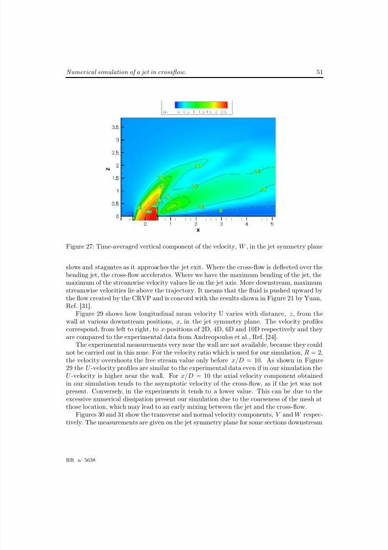
8/10/2019 CFD Numerical simulation of a jet in crossflow..pdf
http://slidepdf.com/reader/full/cfd-numerical-simulation-of-a-jet-in-crossflowpdf 53/83
Numerical simulation of a jet in crossflow. 51
Figure 27: Time-averaged vertical component of the velocity, W , in the jet symmetry plane
slows and stagnates as it approaches the jet exit. Where the cross-flow is deflected over thebending jet, the cross-flow accelerates. Where we have the maximum bending of the jet, themaximum of the streamwise velocity values lie on the jet axis. More downstream, maximum
streamwise velocities lie above the trajectory. It means that the fluid is pushed upward bythe flow created by the CRVP and is concord with the results shown in Figure 21 by Yuan,Ref. [31].
Figure 29 shows how longitudinal mean velocity U varies with distance, z, from thewall at various downstream positions, x, in the jet symmetry plane. The velocity profilescorrespond, from left to right, to x-positions of 2D, 4D, 6D and 10D respectively and theyare compared to the experimental data from Andreopoulos et al., Ref. [24].
The experimental measurements very near the wall are not available, because they couldnot be carried out in this zone. For the velocity ratio which is used for our simulation, R = 2,the velocity overshoots the free stream value only before x/D = 10. As shown in Figure29 the U -velocity profiles are similar to the experimental data even if in our simulation theU -velocity is higher near the wall. For x/D = 10 the axial velocity component obtained
in our simulation tends to the asymptotic velocity of the cross-flow, as if the jet was notpresent. Conversely, in the experiments it tends to a lower value. This can be due to theexcessive numerical dissipation present our simulation due to the coarseness of the mesh atthose location, which may lead to an early mixing between the jet and the cross-flow.
Figures 30 and 31 show the transverse and normal velocity components, V and W respec-tively. The measurements are given on the jet symmetry plane for some sections downstream
RR n° 5638
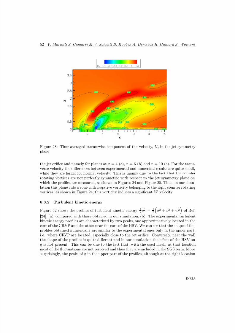
8/10/2019 CFD Numerical simulation of a jet in crossflow..pdf
http://slidepdf.com/reader/full/cfd-numerical-simulation-of-a-jet-in-crossflowpdf 54/83
52 V. Mariotti S. Camarri M.V. Salvetti B. Koobus A. Dervieux H. Guillard S. Wornom
Figure 28: Time-averaged streamwise component of the velocity, U , in the jet symmetryplane
the jet orifice and namely for planes at x = 4 (a), x = 6 (b) and x = 10 (c). For the trans-verse velocity the differences between experimental and numerical results are quite small,
while they are larger for normal velocity. This is mainly due to the fact that the counterrotating vortices are not perfectly symmetric with respect to the jet symmetry plane onwhich the profiles are measured, as shown in Figures 24 and Figure 25. Thus, in our simu-lation this plane cuts a zone with negative vorticity belonging to the right counter rotatingvortices, as shown in Figure 24; this vorticity induces a significant W velocity.
6.3.2 Turbulent kinetic energy
Figure 32 shows the profiles of turbulent kinetic energy 12 q 2 = 1
2
u2 + v2 + w2
of Ref.
[24], (a), compared with those obtained in our simulation, (b). The experimental turbulentkinetic energy profiles are characterized by two peaks, one approximatively located in thecore of the CRVP and the other near the core of the HSV. We can see that the shape of theprofiles obtained numerically are similar to the experimental ones only in the upper part,i.e. where CRVP are located, especially close to the jet orifice. Conversely, near the wallthe shape of the profiles is quite different and in our simulation the effect of the HSV onq is not present. This can be due to the fact that, with the used mesh, at that locationmost of the fluctuations are not resolved and thus they are included in the SGS term. Moresurprisingly, the peaks of q in the upper part of the profiles, although at the right location
INRIA
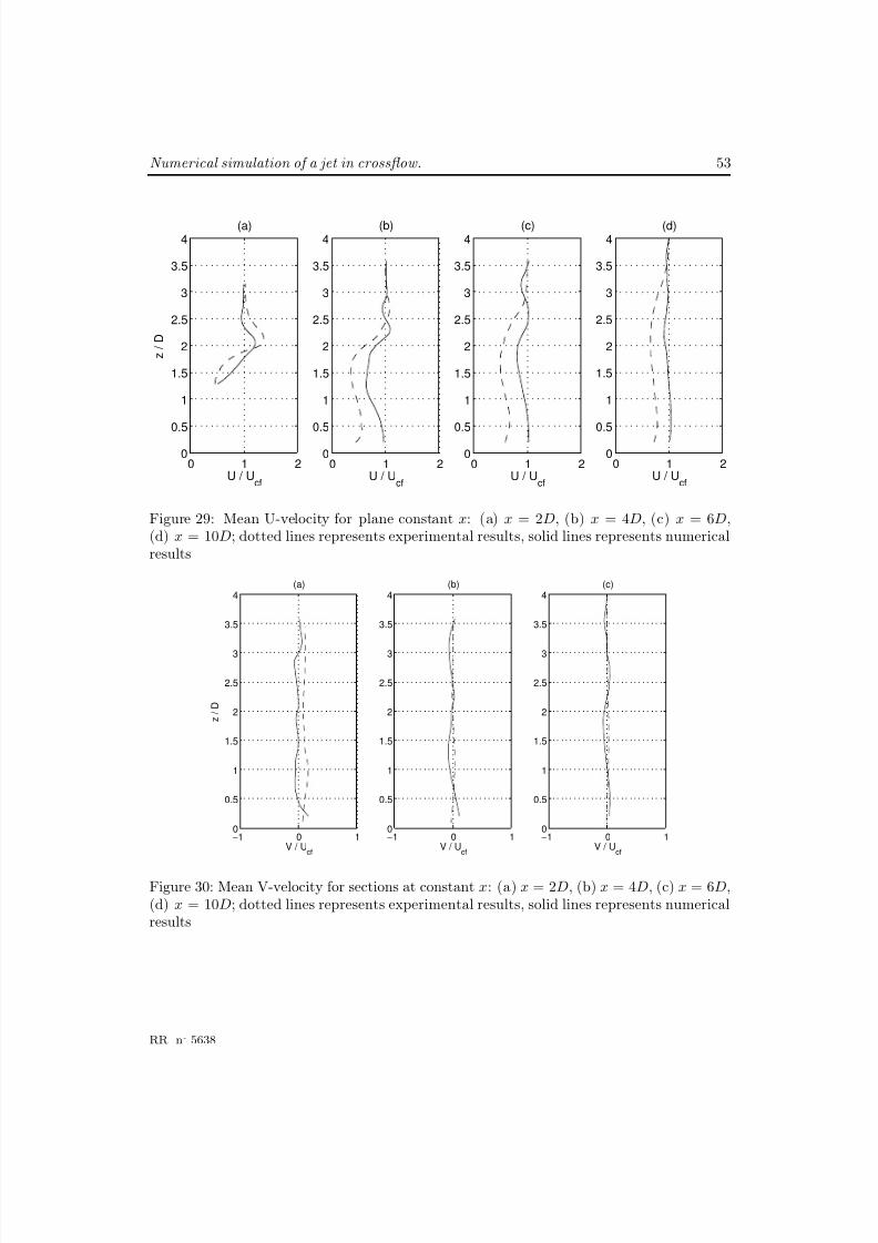
8/10/2019 CFD Numerical simulation of a jet in crossflow..pdf
http://slidepdf.com/reader/full/cfd-numerical-simulation-of-a-jet-in-crossflowpdf 55/83
Numerical simulation of a jet in crossflow. 53
0 1 20
0.5
1
1.5
2
2.5
3
3.5
4
U / Ucf
z / D
(a)
0 1 20
0.5
1
1.5
2
2.5
3
3.5
4
U / Ucf
(b)
0 1 20
0.5
1
1.5
2
2.5
3
3.5
4
U / Ucf
(c)
0 1 20
0.5
1
1.5
2
2.5
3
3.5
4
U / Ucf
(d)
Figure 29: Mean U-velocity for plane constant x: (a) x = 2D, (b) x = 4D, (c) x = 6D,(d) x = 10D; dotted lines represents experimental results, solid lines represents numericalresults
−1 0 10
0.5
1
1.5
2
2.5
3
3.5
4
V / Ucf
z / D
(a)
−1 0 10
0.5
1
1.5
2
2.5
3
3.5
4
V / Ucf
(b)
−1 0 10
0.5
1
1.5
2
2.5
3
3.5
4
V / Ucf
(c)
Figure 30: Mean V-velocity for sections at constant x: (a) x = 2D, (b) x = 4D, (c) x = 6D,(d) x = 10D; dotted lines represents experimental results, solid lines represents numericalresults
RR n° 5638
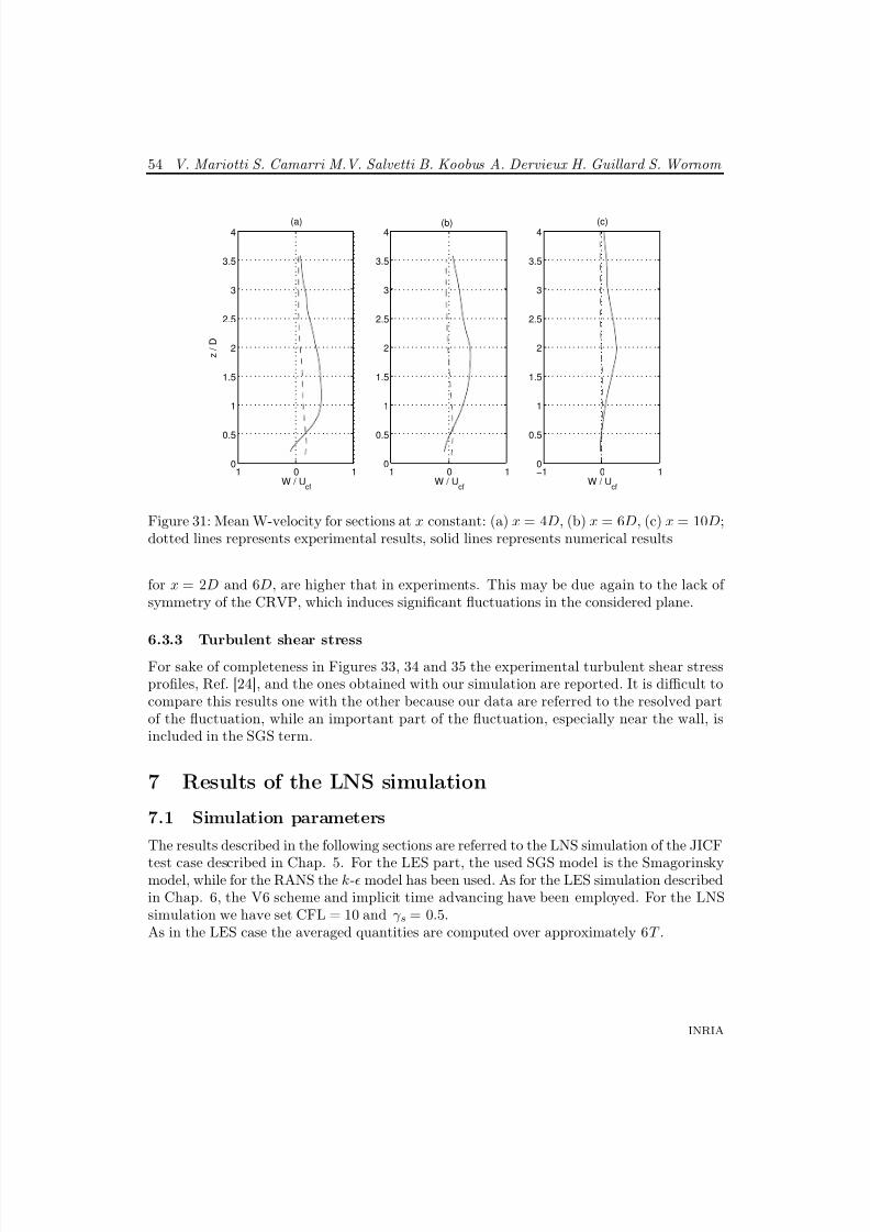
8/10/2019 CFD Numerical simulation of a jet in crossflow..pdf
http://slidepdf.com/reader/full/cfd-numerical-simulation-of-a-jet-in-crossflowpdf 56/83
54 V. Mariotti S. Camarri M.V. Salvetti B. Koobus A. Dervieux H. Guillard S. Wornom
−1 0 10
0.5
1
1.5
2
2.5
3
3.5
4
W / Ucf
z / D
(a)
−1 0 10
0.5
1
1.5
2
2.5
3
3.5
4
W / Ucf
(b)
−1 0 10
0.5
1
1.5
2
2.5
3
3.5
4
W / Ucf
(c)
Figure 31: Mean W-velocity for sections at x constant: (a) x = 4D, (b) x = 6D, (c) x = 10D;dotted lines represents experimental results, solid lines represents numerical results
for x = 2D and 6D, are higher that in experiments. This may be due again to the lack of symmetry of the CRVP, which induces significant fluctuations in the considered plane.
6.3.3 Turbulent shear stressFor sake of completeness in Figures 33, 34 and 35 the experimental turbulent shear stressprofiles, Ref. [24], and the ones obtained with our simulation are reported. It is difficult tocompare this results one with the other because our data are referred to the resolved partof the fluctuation, while an important part of the fluctuation, especially near the wall, isincluded in the SGS term.
7 Results of the LNS simulation
7.1 Simulation parameters
The results described in the following sections are referred to the LNS simulation of the JICF
test case described in Chap. 5. For the LES part, the used SGS model is the Smagorinskymodel, while for the RANS the k- model has been used. As for the LES simulation describedin Chap. 6, the V6 scheme and implicit time advancing have been employed. For the LNSsimulation we have set CFL = 10 and γ s = 0.5.As in the LES case the averaged quantities are computed over approximately 6T .
INRIA
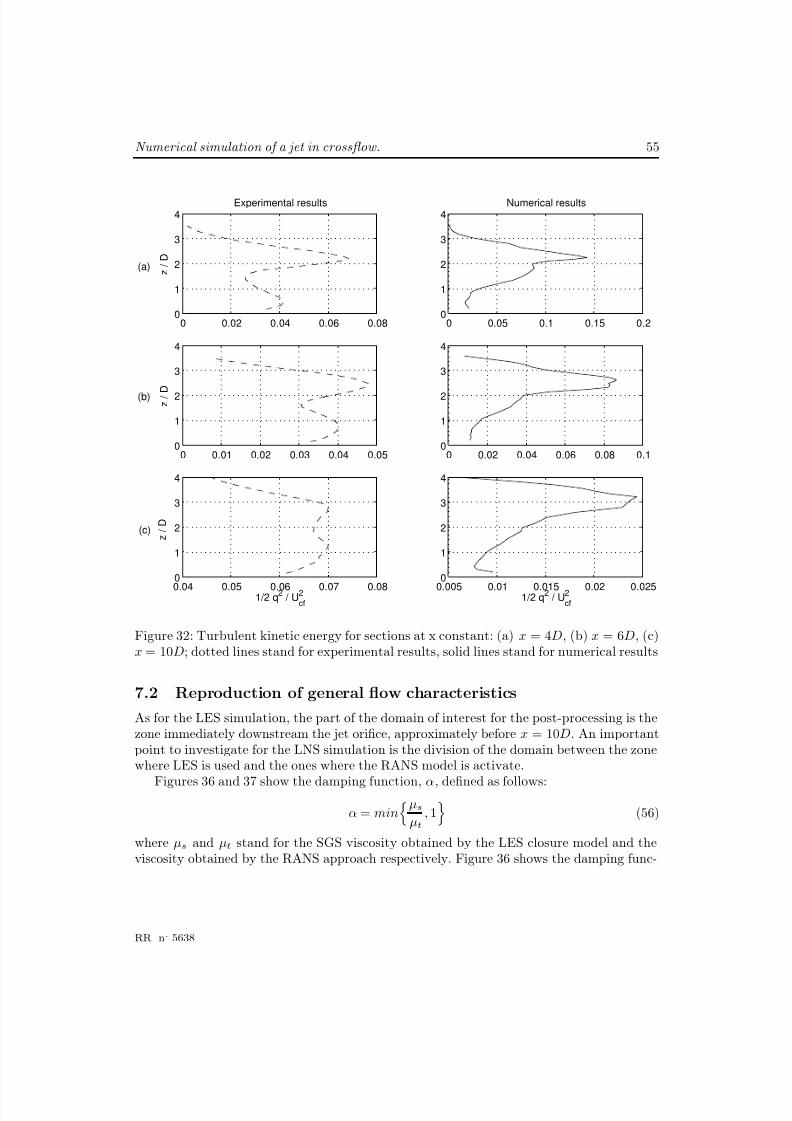
8/10/2019 CFD Numerical simulation of a jet in crossflow..pdf
http://slidepdf.com/reader/full/cfd-numerical-simulation-of-a-jet-in-crossflowpdf 57/83
Numerical simulation of a jet in crossflow. 55
0 0.02 0.04 0.06 0.080
1
2
3
4Experimental results
z / D
0 0.05 0.1 0.15 0.20
1
2
3
4Numerical results
0 0.01 0.02 0.03 0.04 0.050
1
2
3
4
z / D
0 0.02 0.04 0.06 0.08 0.10
1
2
3
4
0.04 0.05 0.06 0.07 0.08
0
1
2
3
4
z / D
1/2 q2 / U
2
cf
0.005 0.01 0.015 0.02 0.025
0
1
2
3
4
1/2 q2 / U
2
cf
(a)
(b)
(c)
Figure 32: Turbulent kinetic energy for sections at x constant: (a) x = 4D, (b) x = 6D, (c)x = 10D; dotted lines stand for experimental results, solid lines stand for numerical results
7.2 Reproduction of general flow characteristics
As for the LES simulation, the part of the domain of interest for the post-processing is thezone immediately downstream the jet orifice, approximately before x = 10D. An importantpoint to investigate for the LNS simulation is the division of the domain between the zonewhere LES is used and the ones where the RANS model is activate.
Figures 36 and 37 show the damping function, α, defined as follows:
α = minµs
µt, 1
(56)
where µs and µt stand for the SGS viscosity obtained by the LES closure model and theviscosity obtained by the RANS approach respectively. Figure 36 shows the damping func-
RR n° 5638
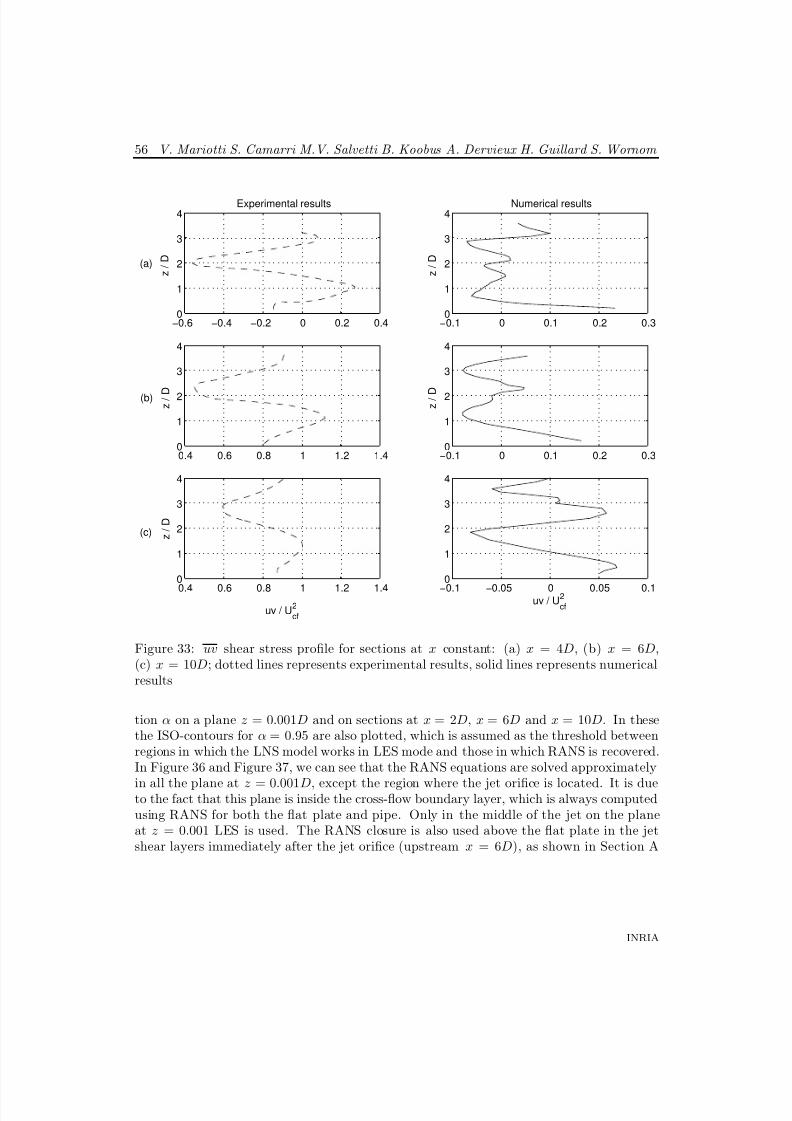
8/10/2019 CFD Numerical simulation of a jet in crossflow..pdf
http://slidepdf.com/reader/full/cfd-numerical-simulation-of-a-jet-in-crossflowpdf 58/83
56 V. Mariotti S. Camarri M.V. Salvetti B. Koobus A. Dervieux H. Guillard S. Wornom
−0.6 −0.4 −0.2 0 0.2 0.40
1
2
3
4Experimental results
z / D
−0.1 0 0.1 0.2 0.30
1
2
3
4
z / D
Numerical results
0.4 0.6 0.8 1 1.2 1.40
1
2
3
4
z / D
−0.1 0 0.1 0.2 0.30
1
2
3
4
z / D
0.4 0.6 0.8 1 1.2 1.4
0
1
2
3
4
uv / U2
cf
z / D
−0.1 −0.05 0 0.05 0.1
0
1
2
3
4
uv / U2
cf
(a)
(b)
(c)
Figure 33: uv shear stress profile for sections at x constant: (a) x = 4D, (b) x = 6D,(c) x = 10D; dotted lines represents experimental results, solid lines represents numericalresults
tion α on a plane z = 0.001D and on sections at x = 2D, x = 6D and x = 10D. In thesethe ISO-contours for α = 0.95 are also plotted, which is assumed as the threshold betweenregions in which the LNS model works in LES mode and those in which RANS is recovered.In Figure 36 and Figure 37, we can see that the RANS equations are solved approximately
in all the plane at z = 0.001D, except the region where the jet orifice is located. It is dueto the fact that this plane is inside the cross-flow boundary layer, which is always computedusing RANS for both the flat plate and pipe. Only in the middle of the jet on the planeat z = 0.001 LES is used. The RANS closure is also used above the flat plate in the jetshear layers immediately after the jet orifice (upstream x = 6D), as shown in Section A
INRIA
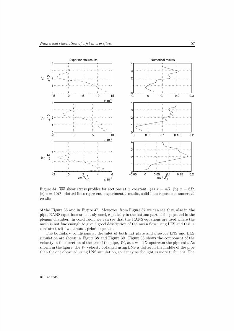
8/10/2019 CFD Numerical simulation of a jet in crossflow..pdf
http://slidepdf.com/reader/full/cfd-numerical-simulation-of-a-jet-in-crossflowpdf 59/83
Numerical simulation of a jet in crossflow. 57
−5 0 5 10 15
x 10−3
0
1
2
3
4
z / D
Experimental results
−0.1 0 0.1 0.2 0.30
1
2
3
4Numerical results
−5 0 5 10
x 10−3
0
1
2
3
4
z / D
0 0.05 0.1 0.15 0.20
1
2
3
4
−2 0 2 4 6
x 10−3
0
2
4
6
z / D
uw / U2
cf
−0.05 0 0.05 0.1 0.15 0.2
0
1
2
3
4
uw / U2
cf
(a)
(b)
(c)
Figure 34: uw shear stress profiles for sections at x constant: (a) x = 4D, (b) x = 6D,(c) x = 10D ; dotted lines represents experimental results, solid lines represents numericalresults
of the Figure 36 and in Figure 37. Moreover, from Figure 37 we can see that, also in thepipe, RANS equations are mainly used, especially in the bottom part of the pipe and in theplenum chamber. In conclusion, we can see that the RANS equations are used where themesh is not fine enough to give a good description of the mean flow using LES and this isconsistent with what was a priori expected.
The boundary conditions at the inlet of both flat plate and pipe for LNS and LESsimulation are shown in Figure 38 and Figure 39. Figure 38 shows the component of thevelocity in the direction of the axe of the pipe, W , at z = −1D upstream the pipe exit. Asshown in the figure, the W velocity obtained using LNS is flatter in the middle of the pipethan the one obtained using LNS simulation, so it may be thought as more turbulent. The
RR n° 5638
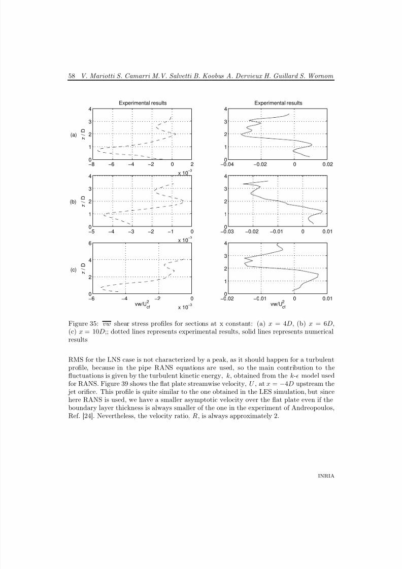
8/10/2019 CFD Numerical simulation of a jet in crossflow..pdf
http://slidepdf.com/reader/full/cfd-numerical-simulation-of-a-jet-in-crossflowpdf 60/83
58 V. Mariotti S. Camarri M.V. Salvetti B. Koobus A. Dervieux H. Guillard S. Wornom
−8 −6 −4 −2 0 2
x 10−3
0
1
2
3
4
z / D
Experimental results
−0.04 −0.02 0 0.020
1
2
3
4Experimental results
−5 −4 −3 −2 −1 0
x 10−3
0
1
2
3
4
z / D
−0.03 −0.02 −0.01 0 0.010
1
2
3
4
−6 −4 −2 0
x 10−3
0
2
4
6
vw/U2
cf
z / D
−0.02 −0.01 0 0.01
0
1
2
3
4
vw/U2
cf
(a)
(b)
(c)
Figure 35: vw shear stress profiles for sections at x constant: (a) x = 4D, (b) x = 6D,(c) x = 10D;; dotted lines represents experimental results, solid lines represents numericalresults
RMS for the LNS case is not characterized by a peak, as it should happen for a turbulentprofile, because in the pipe RANS equations are used, so the main contribution to thefluctuations is given by the turbulent kinetic energy, k, obtained from the k- model usedfor RANS. Figure 39 shows the flat plate streamwise velocity, U , at x = −4D upstream the jet orifice. This profile is quite similar to the one obtained in the LES simulation, but since
here RANS is used, we have a smaller asymptotic velocity over the flat plate even if theboundary layer thickness is always smaller of the one in the experiment of Andreopoulos,Ref. [24]. Nevertheless, the velocity ratio, R, is always approximately 2.
INRIA
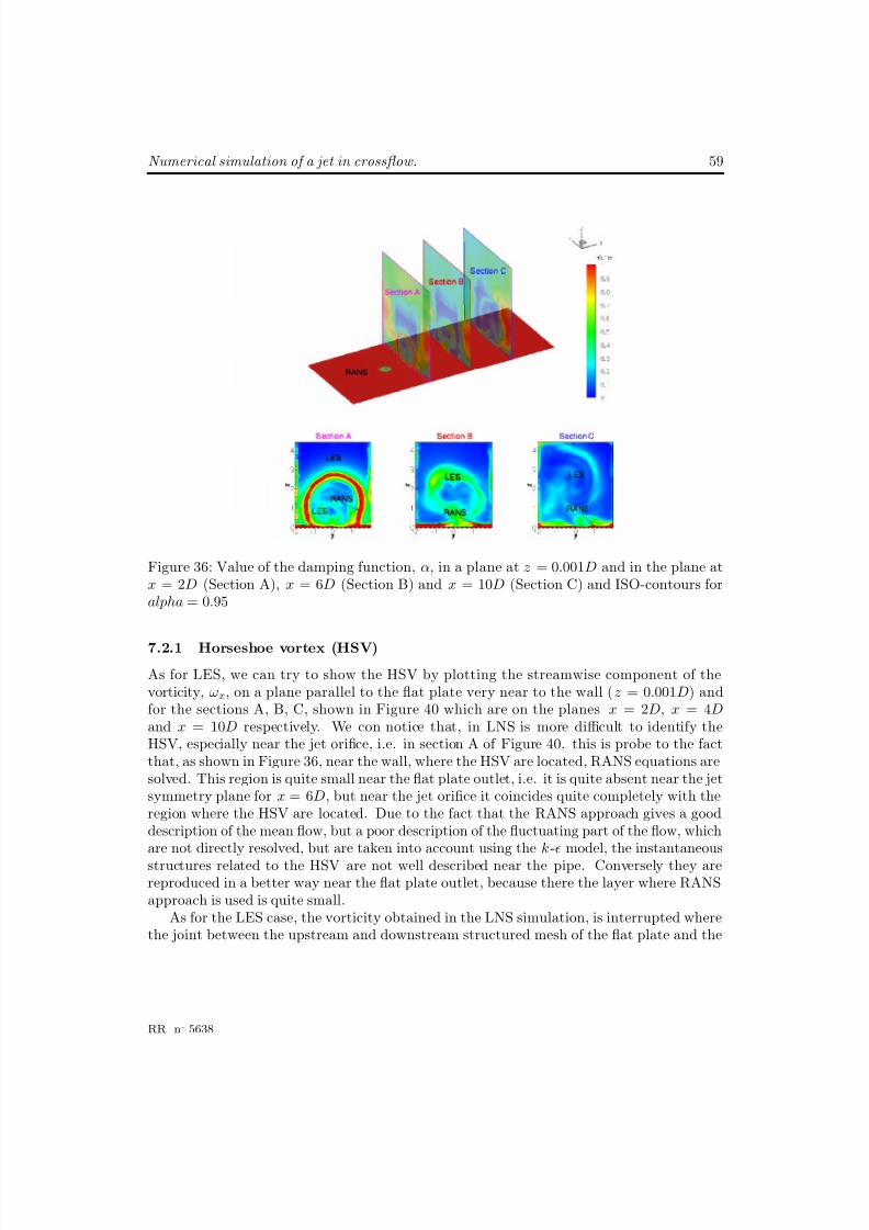
8/10/2019 CFD Numerical simulation of a jet in crossflow..pdf
http://slidepdf.com/reader/full/cfd-numerical-simulation-of-a-jet-in-crossflowpdf 61/83
Numerical simulation of a jet in crossflow. 59
Figure 36: Value of the damping function, α, in a plane at z = 0.001D and in the plane atx = 2D (Section A), x = 6D (Section B) and x = 10D (Section C) and ISO-contours foralpha = 0.95
7.2.1 Horseshoe vortex (HSV)
As for LES, we can try to show the HSV by plotting the streamwise component of thevorticity, ωx, on a plane parallel to the flat plate very near to the wall (z = 0.001D) andfor the sections A, B, C, shown in Figure 40 which are on the planes x = 2D, x = 4Dand x = 10D respectively. We con notice that, in LNS is more difficult to identify theHSV, especially near the jet orifice, i.e. in section A of Figure 40. this is probe to the factthat, as shown in Figure 36, near the wall, where the HSV are located, RANS equations aresolved. This region is quite small near the flat plate outlet, i.e. it is quite absent near the jetsymmetry plane for x = 6D, but near the jet orifice it coincides quite completely with theregion where the HSV are located. Due to the fact that the RANS approach gives a gooddescription of the mean flow, but a poor description of the fluctuating part of the flow, whichare not directly resolved, but are taken into account using the k- model, the instantaneous
structures related to the HSV are not well described near the pipe. Conversely they arereproduced in a better way near the flat plate outlet, because there the layer where RANSapproach is used is quite small.
As for the LES case, the vorticity obtained in the LNS simulation, is interrupted wherethe joint between the upstream and downstream structured mesh of the flat plate and the
RR n° 5638
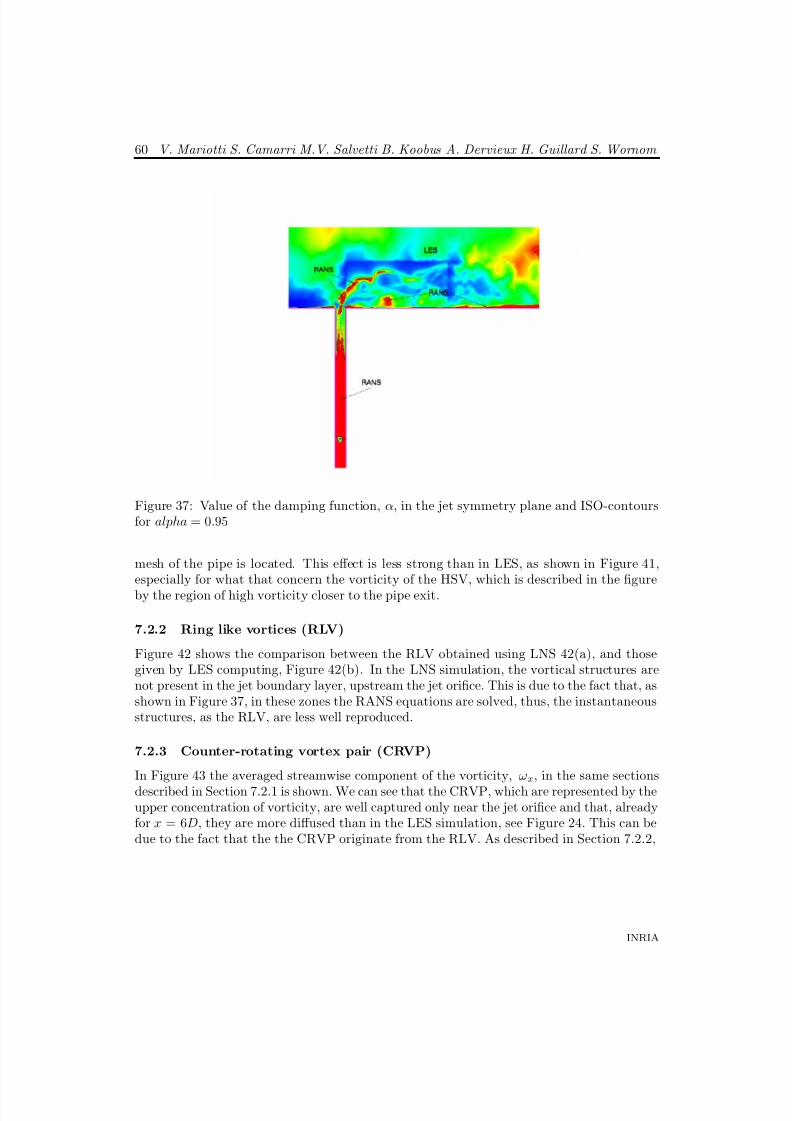
8/10/2019 CFD Numerical simulation of a jet in crossflow..pdf
http://slidepdf.com/reader/full/cfd-numerical-simulation-of-a-jet-in-crossflowpdf 62/83
60 V. Mariotti S. Camarri M.V. Salvetti B. Koobus A. Dervieux H. Guillard S. Wornom
Figure 37: Value of the damping function, α, in the jet symmetry plane and ISO-contoursfor alpha = 0.95
mesh of the pipe is located. This effect is less strong than in LES, as shown in Figure 41,especially for what that concern the vorticity of the HSV, which is described in the figureby the region of high vorticity closer to the pipe exit.
7.2.2 Ring like vortices (RLV)
Figure 42 shows the comparison between the RLV obtained using LNS 42(a), and thosegiven by LES computing, Figure 42(b). In the LNS simulation, the vortical structures arenot present in the jet boundary layer, upstream the jet orifice. This is due to the fact that, asshown in Figure 37, in these zones the RANS equations are solved, thus, the instantaneousstructures, as the RLV, are less well reproduced.
7.2.3 Counter-rotating vortex pair (CRVP)
In Figure 43 the averaged streamwise component of the vorticity, ωx, in the same sectionsdescribed in Section 7.2.1 is shown. We can see that the CRVP, which are represented by theupper concentration of vorticity, are well captured only near the jet orifice and that, alreadyfor x = 6D, they are more diffused than in the LES simulation, see Figure 24. This can bedue to the fact that the the CRVP originate from the RLV. As described in Section 7.2.2,
INRIA
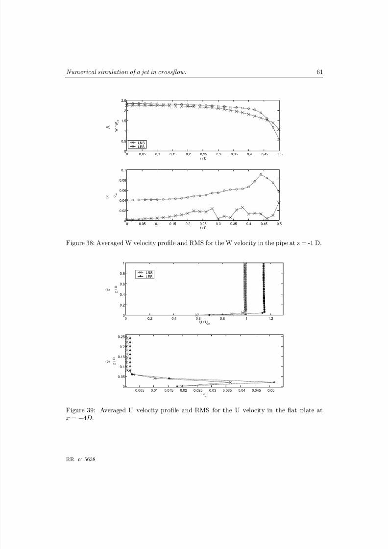
8/10/2019 CFD Numerical simulation of a jet in crossflow..pdf
http://slidepdf.com/reader/full/cfd-numerical-simulation-of-a-jet-in-crossflowpdf 63/83
Numerical simulation of a jet in crossflow. 61
0 0.05 0.1 0.15 0.2 0.25 0.3 0.35 0.4 0.45 0.50
0.5
1
1.5
2
2.5
r / D
W /
W c f
0 0.05 0.1 0.15 0.2 0.25 0.3 0.35 0.4 0.45 0.50
0.02
0.04
0.06
0.08
0.1
σ w
r / D
LNSLES
(a)
(b)
Figure 38: Averaged W velocity profile and RMS for the W velocity in the pipe at z = -1 D.
0 0.2 0.4 0.6 0.8 1 1.20
0.2
0.4
0.6
0.8
1
U / Ucf
z / D
0.005 0.01 0.015 0.02 0.025 0.03 0.035 0.04 0.045 0.05
0
0.05
0.1
0.15
0.2
0.25
σu
z / D
LNSLES
(a)
(b)
Figure 39: Averaged U velocity profile and RMS for the U velocity in the flat plate atx = −4D.
RR n° 5638
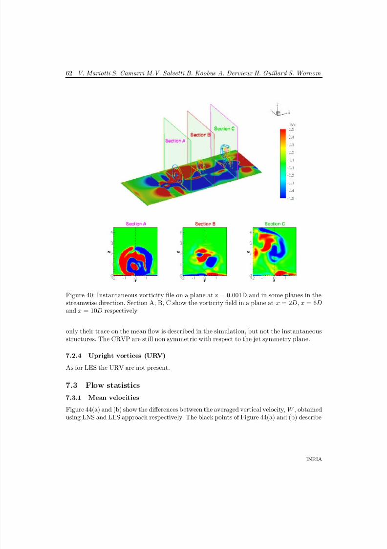
8/10/2019 CFD Numerical simulation of a jet in crossflow..pdf
http://slidepdf.com/reader/full/cfd-numerical-simulation-of-a-jet-in-crossflowpdf 64/83
62 V. Mariotti S. Camarri M.V. Salvetti B. Koobus A. Dervieux H. Guillard S. Wornom
Figure 40: Instantaneous vorticity file on a plane at z = 0.001D and in some planes in thestreamwise direction. Section A, B, C show the vorticity field in a plane at x = 2D, x = 6Dand x = 10D respectively
only their trace on the mean flow is described in the simulation, but not the instantaneousstructures. The CRVP are still non symmetric with respect to the jet symmetry plane.
7.2.4 Upright vortices (URV)
As for LES the URV are not present.
7.3 Flow statistics
7.3.1 Mean velocities
Figure 44(a) and (b) show the differences between the averaged vertical velocity, W , obtainedusing LNS and LES approach respectively. The black points of Figure 44(a) and (b) describe
INRIA
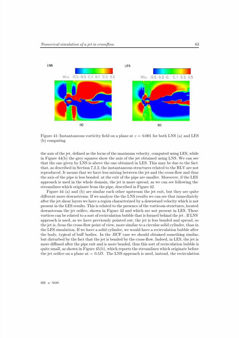
8/10/2019 CFD Numerical simulation of a jet in crossflow..pdf
http://slidepdf.com/reader/full/cfd-numerical-simulation-of-a-jet-in-crossflowpdf 65/83
Numerical simulation of a jet in crossflow. 63
Figure 41: Instantaneous vorticity field on a plane at z = 0.001 for both LNS (a) and LES(b) computing
the axis of the jet, defined as the locus of the maximum velocity, computed using LES, whilein Figure 44(b) the grey squares show the axis of the jet obtained using LNS. We can seethat the one given by LNS is above the one obtained in LES. This may be due to the factthat, as described in Section 7.2.2, the instantaneous structures related to the RLV are notreproduced. It means that we have less mixing between the jet and the cross-flow and thus
the axis of the pipe is less bended. at the exit of the pipe are smaller. Moreover, if the LESapproach is used in the whole domain, the jet is more spread, as we can see following thestreamlines which originate from the pipe, described in Figure 42.
Figure 44 (a) and (b) are similar each other upstream the jet exit, but they are quitedifferent more downstream. If we analyze the the LNS results we can see that immediatelyafter the jet shear layers we have a region characterized by a downward velocity which is notpresent in the LES results. This is related to the presence of the vorticous structures, locateddownstream the jet orifice, shown in Figure 42 and which are not present in LES. Thesevortices can be related to a sort of recirculation bubble that is formed behind the jet . If LNSapproach is used, as we have previously pointed out, the jet is less bended and spread, sothe jet is, from the cross-flow point of view, more similar to a circular solid cylinder, than inthe LES simulation. If we have a solid cylinder, we would have a recirculation bubble afterthe body, typical of buff bodies. In the JICF case we should obtained something similar,but disturbed by the fact that the jet is bended by the cross-flow. Indeed, in LES, the jet ismore diffused after the pipe exit and is more bended, thus this sort of recirculation bubble isquite small, as shown in Figure 45(b), which reports the streamlines which originate beforethe jet orifice on a plane at = 0.5D. The LNS approach is used, instead, the recirculation
RR n° 5638
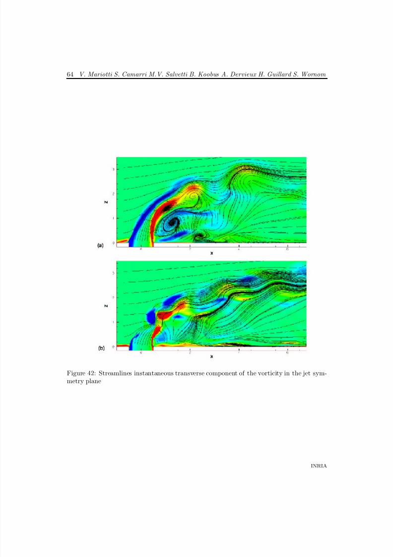
8/10/2019 CFD Numerical simulation of a jet in crossflow..pdf
http://slidepdf.com/reader/full/cfd-numerical-simulation-of-a-jet-in-crossflowpdf 66/83
64 V. Mariotti S. Camarri M.V. Salvetti B. Koobus A. Dervieux H. Guillard S. Wornom
Figure 42: Streamlines instantaneous transverse component of the vorticity in the jet sym-metry plane
INRIA
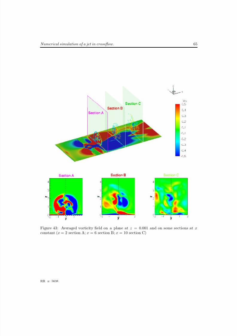
8/10/2019 CFD Numerical simulation of a jet in crossflow..pdf
http://slidepdf.com/reader/full/cfd-numerical-simulation-of-a-jet-in-crossflowpdf 67/83
Numerical simulation of a jet in crossflow. 65
Figure 43: Averaged vorticity field on a plane at z = 0.001 and on some sections at xconstant (x = 2 section A; x = 6 section B; x = 10 section C)
RR n° 5638
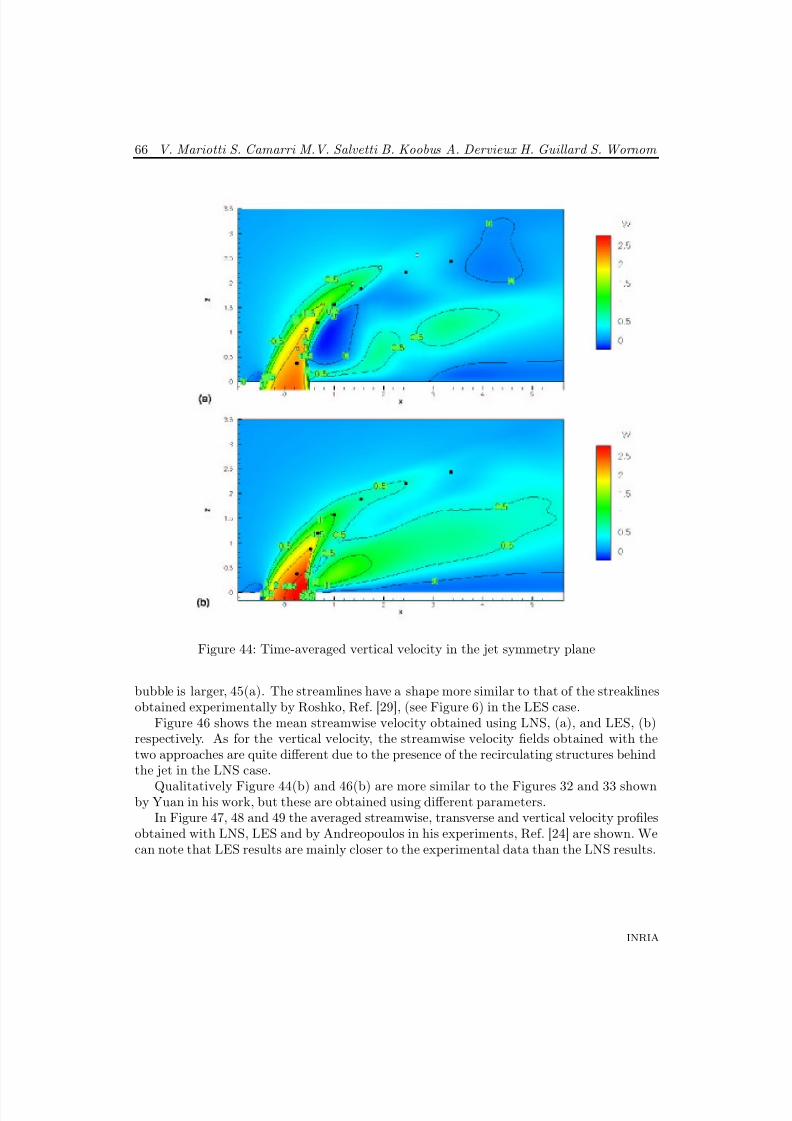
8/10/2019 CFD Numerical simulation of a jet in crossflow..pdf
http://slidepdf.com/reader/full/cfd-numerical-simulation-of-a-jet-in-crossflowpdf 68/83
66 V. Mariotti S. Camarri M.V. Salvetti B. Koobus A. Dervieux H. Guillard S. Wornom
Figure 44: Time-averaged vertical velocity in the jet symmetry plane
bubble is larger, 45(a). The streamlines have a shape more similar to that of the streaklinesobtained experimentally by Roshko, Ref. [29], (see Figure 6) in the LES case.
Figure 46 shows the mean streamwise velocity obtained using LNS, (a), and LES, (b)respectively. As for the vertical velocity, the streamwise velocity fields obtained with thetwo approaches are quite different due to the presence of the recirculating structures behindthe jet in the LNS case.
Qualitatively Figure 44(b) and 46(b) are more similar to the Figures 32 and 33 shownby Yuan in his work, but these are obtained using different parameters.
In Figure 47, 48 and 49 the averaged streamwise, transverse and vertical velocity profilesobtained with LNS, LES and by Andreopoulos in his experiments, Ref. [24] are shown. Wecan note that LES results are mainly closer to the experimental data than the LNS results.
INRIA
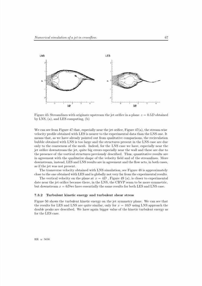
8/10/2019 CFD Numerical simulation of a jet in crossflow..pdf
http://slidepdf.com/reader/full/cfd-numerical-simulation-of-a-jet-in-crossflowpdf 69/83
Numerical simulation of a jet in crossflow. 67
Figure 45: Streamlines with originate upstream the jet orifice in a plane z = 0.5D obtainedby LNS, (a), and LES computing, (b)
We can see from Figure 47 that, especially near the jet orifice, Figure 47(a), the stream-wisevelocity profile obtained with LES is nearer to the experimental data than the LNS one. Itmeans that, as we have already pointed out from qualitative comparisons, the recirculationbubble obtained with LNS is too large and the structures present in the LNS case are dueonly to the coarseness of the mesh. Indeed, for the LNS case we have, especially near the
jet orifice downstream the jet, quite big errors especially near the wall and these are due tothe presence of the vortical structures previously described. Thus, quantitative results arein agreement with the qualitative shape of the velocity field and of the streamlines. Moredownstream, instead, LES and LNS results are in agreement and the flow acts, in both cases,as if the jet was not present.
The transverse velocity obtained with LNS simulation, see Figure 48 is approximatelyclose to the one obtained with LES and is globally not very far from the experimental results.
The vertical velocity on the plane at x = 4D , Figure 49 (a), is closer to experimentaldate near the jet orifice because there, in the LNS, the CRVP seam to be more symmetric,but downstream x = 6Dwe have essentially the same results for both LES and LNS case.
7.3.2 Turbulent kinetic energy and turbulent shear stress
Figure 50 shows the turbulent kinetic energy on the jet symmetry plane. We can see thatthe results for LES and LNS are quite similar, only for x = 10D using LNS approach thedouble peaks are described. We have again bigger value of the kinetic turbulent energy asfor the LES case.
RR n° 5638
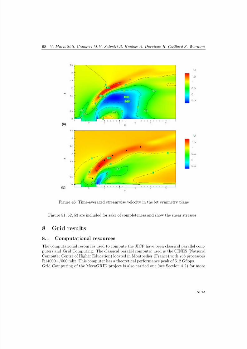
8/10/2019 CFD Numerical simulation of a jet in crossflow..pdf
http://slidepdf.com/reader/full/cfd-numerical-simulation-of-a-jet-in-crossflowpdf 70/83
68 V. Mariotti S. Camarri M.V. Salvetti B. Koobus A. Dervieux H. Guillard S. Wornom
Figure 46: Time-averaged streamwise velocity in the jet symmetry plane
Figure 51, 52, 53 are included for sake of completeness and show the shear stresses.
8 Grid results
8.1 Computational resources
The computational resources used to compute the JICF have been classical parallel com-puters and Grid Computing. The classical parallel computer used is the CINES (NationalComputer Centre of Higher Education) located in Montpellier (France),with 768 processorsR14000+/500 mhz. This computer has a theoretical performance peak of 512 Gflops.Grid Computing of the MecaGRID project is also carried out (see Section 4.2) for more
INRIA
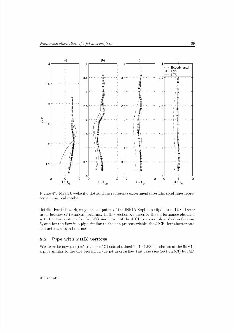
8/10/2019 CFD Numerical simulation of a jet in crossflow..pdf
http://slidepdf.com/reader/full/cfd-numerical-simulation-of-a-jet-in-crossflowpdf 71/83
Numerical simulation of a jet in crossflow. 69
−2 0 2
1.5
2
2.5
3
3.5
4
U / Ucf
z / D
(a)
0 1 20
0.5
1
1.5
2
2.5
3
3.5
4
U / Ucf
(b)
0 1 20
0.5
1
1.5
2
2.5
3
3.5
4
U / Ucf
(c)
0 1 20
0.5
1
1.5
2
2.5
3
3.5
4
U / Ucf
(d)
ExperimentalLNSLES
Figure 47: Mean U-velocity; dotted lines represents experimental results, solid lines repre-sents numerical results
details. For this work, only the computers of the INRIA Sophia-Antipolis and IUSTI wereused, because of technical problems. In this section we describe the performance obtainedwith the two systems for the LES simulation of the JICF test case, described in Section5, and for the flow in a pipe similar to the one present within the JICF, but shorter andcharacterized by a finer mesh.
8.2 Pipe with 241K vertices
We describe now the performance of Globus obtained in the LES simulation of the flow ina pipe similar to the one present in the jet in crossflow test case (see Section 5.3) but 5D
RR n° 5638
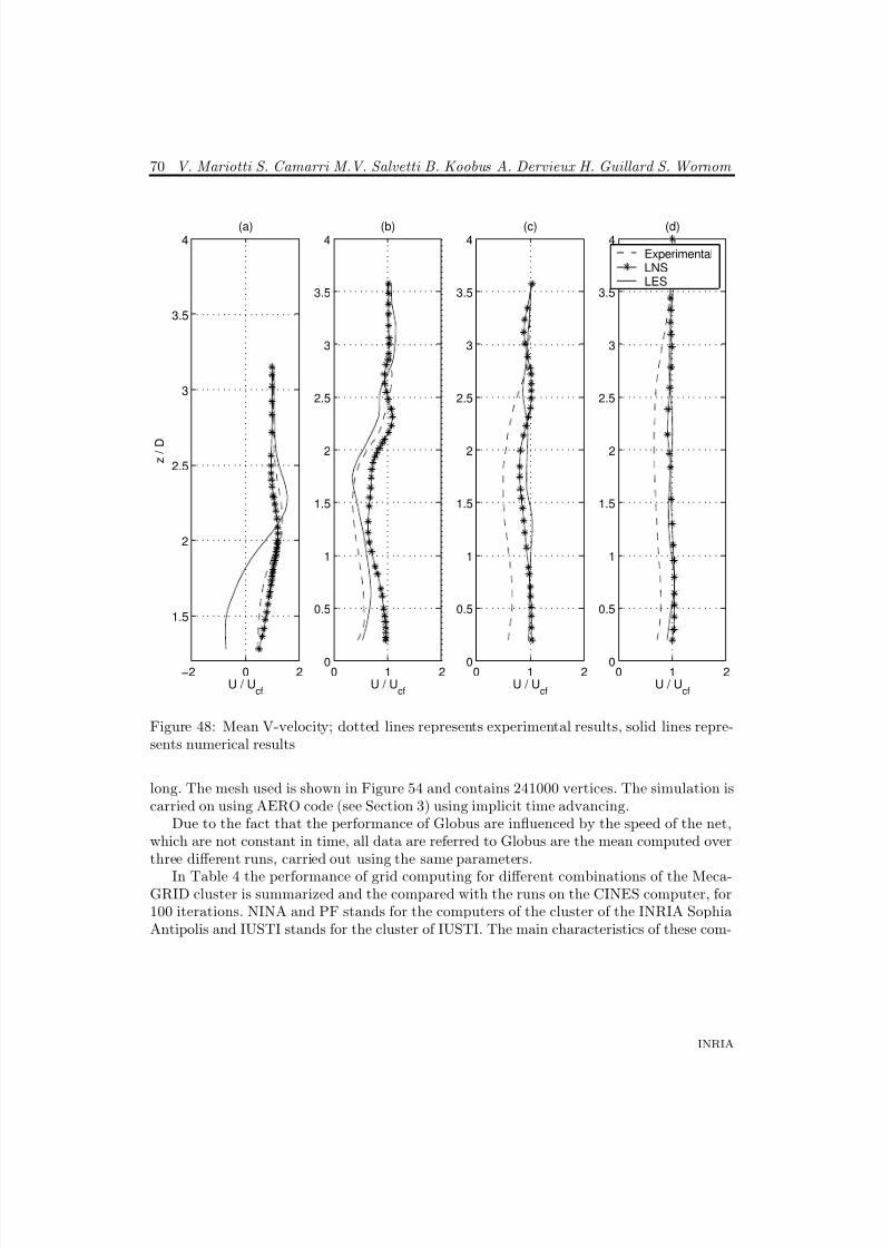
8/10/2019 CFD Numerical simulation of a jet in crossflow..pdf
http://slidepdf.com/reader/full/cfd-numerical-simulation-of-a-jet-in-crossflowpdf 72/83
70 V. Mariotti S. Camarri M.V. Salvetti B. Koobus A. Dervieux H. Guillard S. Wornom
−2 0 2
1.5
2
2.5
3
3.5
4
U / Ucf
z / D
(a)
0 1 20
0.5
1
1.5
2
2.5
3
3.5
4
U / Ucf
(b)
0 1 20
0.5
1
1.5
2
2.5
3
3.5
4
U / Ucf
(c)
0 1 20
0.5
1
1.5
2
2.5
3
3.5
4
U / Ucf
(d)
ExperimentalLNSLES
Figure 48: Mean V-velocity; dotted lines represents experimental results, solid lines repre-sents numerical results
long. The mesh used is shown in Figure 54 and contains 241000 vertices. The simulation iscarried on using AERO code (see Section 3) using implicit time advancing.
Due to the fact that the performance of Globus are influenced by the speed of the net,which are not constant in time, all data are referred to Globus are the mean computed overthree different runs, carried out using the same parameters.
In Table 4 the performance of grid computing for different combinations of the Meca-GRID cluster is summarized and the compared with the runs on the CINES computer, for100 iterations. NINA and PF stands for the computers of the cluster of the INRIA SophiaAntipolis and IUSTI stands for the cluster of IUSTI. The main characteristics of these com-
INRIA
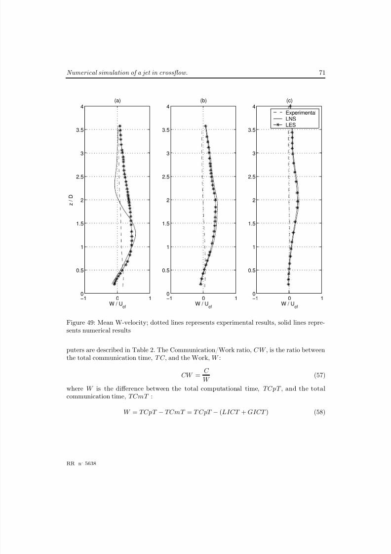
8/10/2019 CFD Numerical simulation of a jet in crossflow..pdf
http://slidepdf.com/reader/full/cfd-numerical-simulation-of-a-jet-in-crossflowpdf 73/83
Numerical simulation of a jet in crossflow. 71
−1 0 10
0.5
1
1.5
2
2.5
3
3.5
4
W / Ucf
z / D
(a)
−1 0 10
0.5
1
1.5
2
2.5
3
3.5
4
W / Ucf
(b)
−1 0 10
0.5
1
1.5
2
2.5
3
3.5
4
W / Ucf
(c)
ExperimentalLNSLES
Figure 49: Mean W-velocity; dotted lines represents experimental results, solid lines repre-sents numerical results
puters are described in Table 2. The Communication/Work ratio, C W , is the ratio betweenthe total communication time, T C , and the Work, W :
CW = C
W (57)
where W is the difference between the total computational time, TCpT , and the totalcommunication time, TCmT :
W = TCpT − TCmT = T CpT − (LICT + GICT ) (58)
RR n° 5638
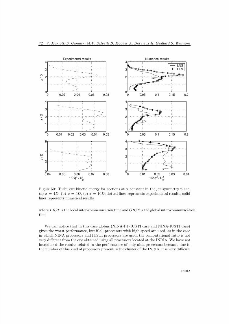
8/10/2019 CFD Numerical simulation of a jet in crossflow..pdf
http://slidepdf.com/reader/full/cfd-numerical-simulation-of-a-jet-in-crossflowpdf 74/83
72 V. Mariotti S. Camarri M.V. Salvetti B. Koobus A. Dervieux H. Guillard S. Wornom
0 0.02 0.04 0.06 0.080
1
2
3
4Experimental results
z / D
0 0.05 0.1 0.15 0.20
1
2
3
4Numerical results
0 0.01 0.02 0.03 0.04 0.050
1
2
3
4
z / D
0 0.05 0.1 0.15 0.20
1
2
3
4
0.04 0.05 0.06 0.07 0.080
2
4
6
z / D
1/2 q2 / U
2
cf
0 0.01 0.02 0.03 0.040
1
2
3
4
1/2 q2 / U
2
cf
LNS
LES
Figure 50: Turbulent kinetic energy for sections at x constant in the jet symmetry plane:(a) x = 4D, (b) x = 6D, (c) x = 10D; dotted lines represents experimental results, solidlines represents numerical results
where LICT is the local inter-communication time and GICT is the global inter-communicationtime
We can notice that in this case globus (NINA-PF-IUSTI case and NINA-IUSTI case)gives the worst performance, but if all processors with high speed are used, as in the casein which NINA processors and IUSTI processors are used, the computational ratio is notvery different from the one obtained using all processors located at the INRIA. We have notintroduced the results related to the performance of only nina processors because, due tothe number of this kind of processors present in the cluster of the INRIA, it is very difficult
INRIA
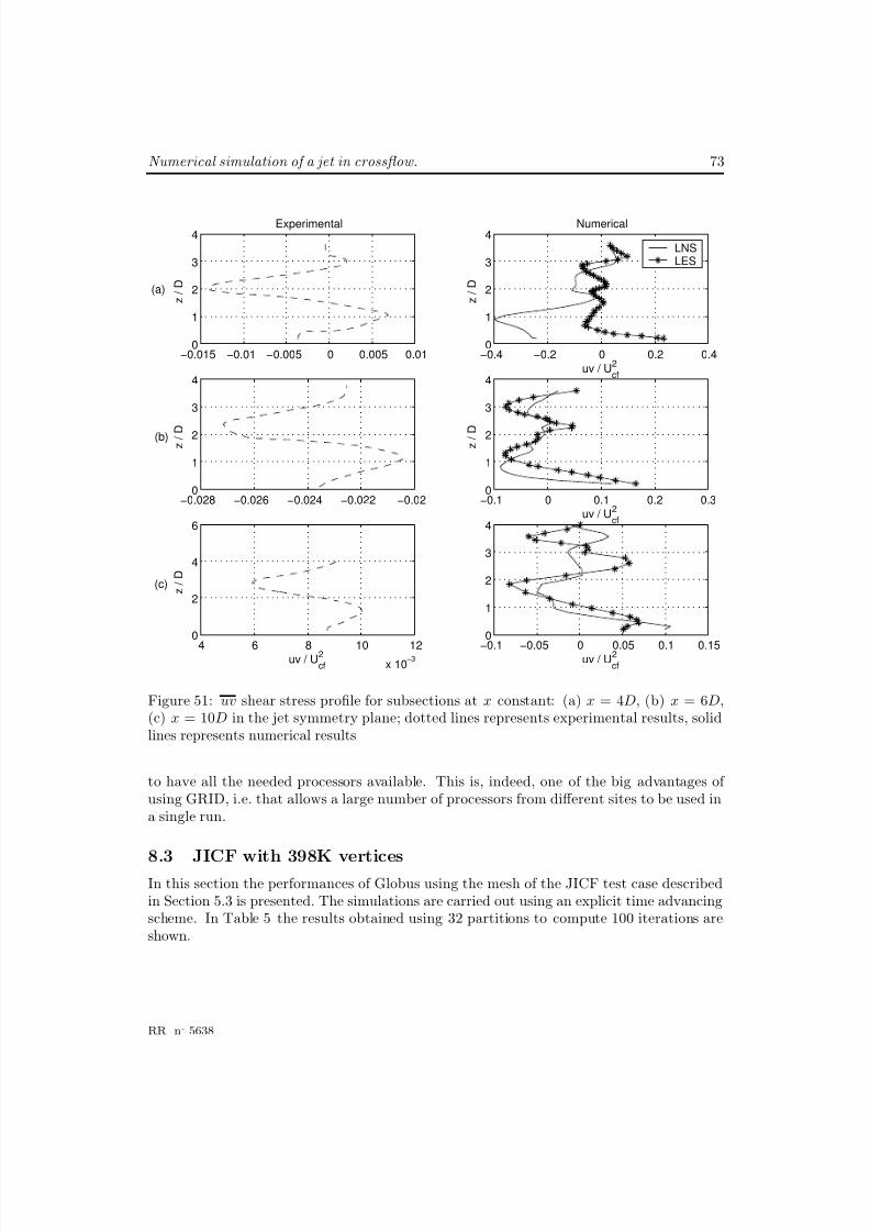
8/10/2019 CFD Numerical simulation of a jet in crossflow..pdf
http://slidepdf.com/reader/full/cfd-numerical-simulation-of-a-jet-in-crossflowpdf 75/83
Numerical simulation of a jet in crossflow. 73
−0.015 −0.01 −0.005 0 0.005 0.010
1
2
3
4
z / D
Experimental
−0.4 −0.2 0 0.2 0.40
1
2
3
4
z / D
uv / U2
cf
Numerical
−0.028 −0.026 −0.024 −0.022 −0.020
1
2
3
4
z / D
−0.1 0 0.1 0.2 0.30
1
2
3
4
uv / U2
cf
z / D
4 6 8 10 12
x 10−3
0
2
4
6
uv / U2
cf
z / D
−0.1 −0.05 0 0.05 0.1 0.15
0
1
2
3
4
uv / U2
cf
LNSLES
(a)
(b)
(c)
Figure 51: uv shear stress profile for subsections at x constant: (a) x = 4D, (b) x = 6D,(c) x = 10D in the jet symmetry plane; dotted lines represents experimental results, solidlines represents numerical results
to have all the needed processors available. This is, indeed, one of the big advantages of using GRID, i.e. that allows a large number of processors from different sites to be used ina single run.
8.3 JICF with 398K verticesIn this section the performances of Globus using the mesh of the JICF test case describedin Section 5.3 is presented. The simulations are carried out using an explicit time advancingscheme. In Table 5 the results obtained using 32 partitions to compute 100 iterations areshown.
RR n° 5638
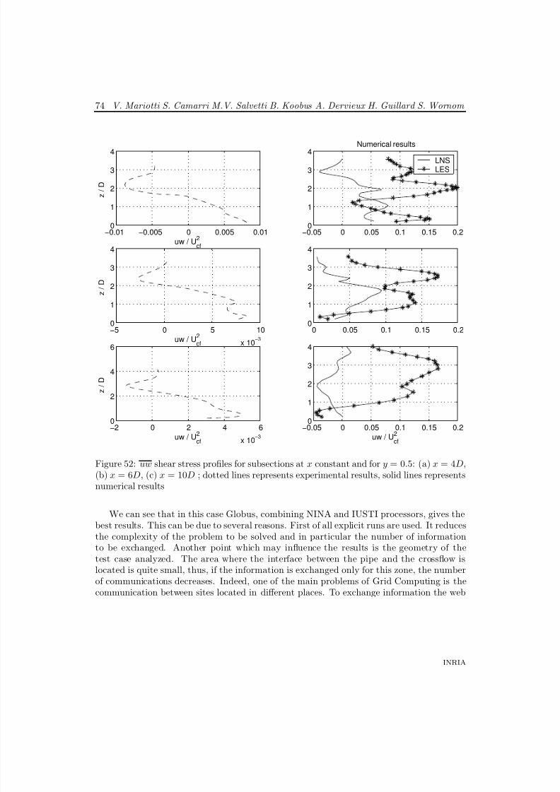
8/10/2019 CFD Numerical simulation of a jet in crossflow..pdf
http://slidepdf.com/reader/full/cfd-numerical-simulation-of-a-jet-in-crossflowpdf 76/83
74 V. Mariotti S. Camarri M.V. Salvetti B. Koobus A. Dervieux H. Guillard S. Wornom
−0.01 −0.005 0 0.005 0.010
1
2
3
4
z / D
uw / U2
cf
−0.05 0 0.05 0.1 0.15 0.20
1
2
3
4
Numerical results
−5 0 5 10
x 10−3
0
1
2
3
4
z / D
uw / U2
cf
0 0.05 0.1 0.15 0.20
1
2
3
4
−2 0 2 4 6
x 10−3
0
2
4
6
z / D
uw / U2
cf
−0.05 0 0.05 0.1 0.15 0.20
1
2
3
4
uw / U2
cf
LNS
LES
Figure 52: uw shear stress profiles for subsections at x constant and for y = 0.5: (a) x = 4D,(b) x = 6D, (c) x = 10D ; dotted lines represents experimental results, solid lines representsnumerical results
We can see that in this case Globus, combining NINA and IUSTI processors, gives thebest results. This can be due to several reasons. First of all explicit runs are used. It reducesthe complexity of the problem to be solved and in particular the number of informationto be exchanged. Another point which may influence the results is the geometry of thetest case analyzed. The area where the interface between the pipe and the crossflow islocated is quite small, thus, if the information is exchanged only for this zone, the numberof communications decreases. Indeed, one of the main problems of Grid Computing is thecommunication between sites located in different places. To exchange information the web
INRIA
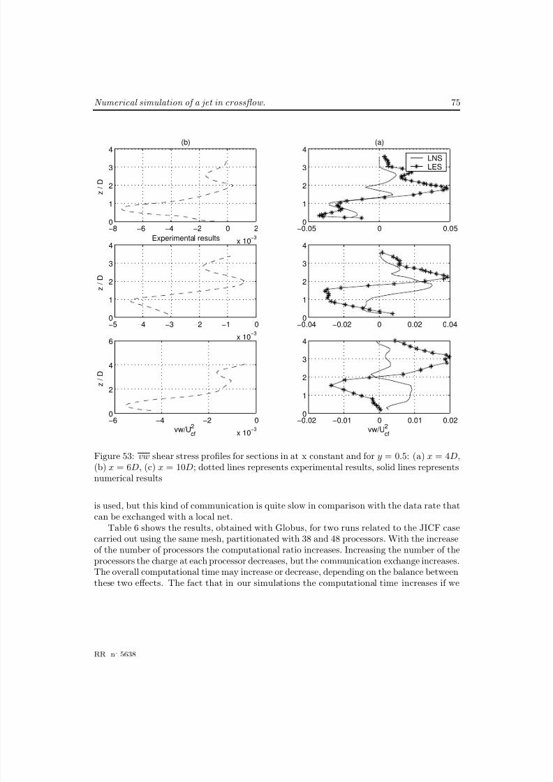
8/10/2019 CFD Numerical simulation of a jet in crossflow..pdf
http://slidepdf.com/reader/full/cfd-numerical-simulation-of-a-jet-in-crossflowpdf 77/83
Numerical simulation of a jet in crossflow. 75
−8 −6 −4 −2 0 2
x 10−3
0
1
2
3
4
z / D
(b)
−0.05 0 0.050
1
2
3
4(a)
−5 −4 −3 −2 −1 0
x 10−3
0
1
2
3
4Experimental results
z / D
−0.04 −0.02 0 0.02 0.040
1
2
3
4
−6 −4 −2 0
x 10−3
0
2
4
6
vw/U2
cf
z / D
−0.02 −0.01 0 0.01 0.020
1
2
3
4
vw/U2
cf
LNS
LES
Figure 53: vw shear stress profiles for sections in at x constant and for y = 0.5: (a) x = 4D,(b) x = 6D, (c) x = 10D; dotted lines represents experimental results, solid lines representsnumerical results
is used, but this kind of communication is quite slow in comparison with the data rate thatcan be exchanged with a local net.
Table 6 shows the results, obtained with Globus, for two runs related to the JICF casecarried out using the same mesh, partitionated with 38 and 48 processors. With the increase
of the number of processors the computational ratio increases. Increasing the number of theprocessors the charge at each processor decreases, but the communication exchange increases.The overall computational time may increase or decrease, depending on the balance betweenthese two effects. The fact that in our simulations the computational time increases if we
RR n° 5638
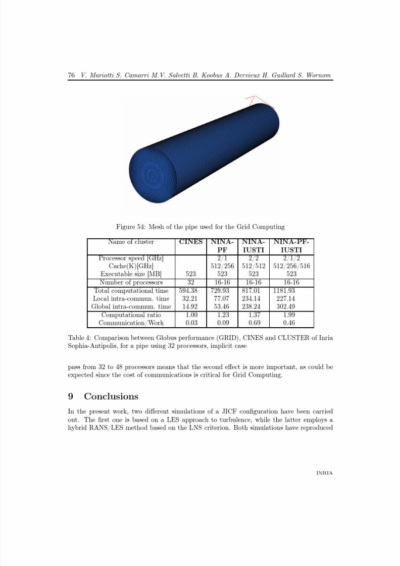
8/10/2019 CFD Numerical simulation of a jet in crossflow..pdf
http://slidepdf.com/reader/full/cfd-numerical-simulation-of-a-jet-in-crossflowpdf 78/83
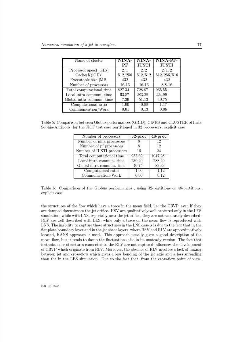
8/10/2019 CFD Numerical simulation of a jet in crossflow..pdf
http://slidepdf.com/reader/full/cfd-numerical-simulation-of-a-jet-in-crossflowpdf 79/83
8/10/2019 CFD Numerical simulation of a jet in crossflow..pdf
http://slidepdf.com/reader/full/cfd-numerical-simulation-of-a-jet-in-crossflowpdf 80/83
78 V. Mariotti S. Camarri M.V. Salvetti B. Koobus A. Dervieux H. Guillard S. Wornom
the jet is similar to an obstacle, if the jet is less bended and spread, it is more similar to asolid cylinder. Thus implies that the recirculation bubble, which is formed behind the jet, islarger than in LES and in experiments and that behind the jet are present some structuresthat are not present in the experiments. Consequently, in these regions the velocity profilesare less close to the experimental results than those obtained in LES.
The results obtained in the LES simulation are qualitatively more similar to the experi-mental results than the ones obtained with LNS. The largest errors are present near the wall,where the mesh is not fine enough to accurately capture the HSV vortices. Downstream the jet orifice, near the flat plate outlet, the flow obtained in the simulations is quicker than inthe experiments and, near the wall, it acts as the jet was not present. This is still due tothe coarseness of the mesh especially near the wall. Moreover the presence of a preferentialdirection in the grid, due to the fact that the tetrahedron of the mesh are all cut in the same
direction, makes CRVP not perfectly symmetric. This gives a significant vertical componentof the velocity on the jet symmetry plane, which is not found in the experiments.
The errors in the mean velocity profiles can be also due to the different inflow conditionsbetween simulations and experiments and to the value of the velocity ratio that, which isnot exactly 2. In the future the Reichardt velocity profile can be used as inflow conditionfor the cross-flow and a finer mesh especially near the wall should be used.
As for Grid Computing, we have obtained good results in the simulation of JICF, forwhich Grid Computing has been found to work better than classical clusters. This can bedue to the geometry of the test case, which is particularly suitable for this kind of computing,or to the fact that explicit time advancing was used, which needs less data exchange. Indeed,the main problem in Grid Computing is the exchange of communications betweenprocessorslocated in different sites, which is realized through the web. Conversely, the main advantageof Grid Computing is the possibility to use a large number of processors, using existingprocessors allocated in different sites. For example, to run the JICF simulation, we haveused 32 processors and we had some problems in carrying out the simulation using only thecluster of the INRIA, because the quantity of memory per node needed for our simulationwas available only for one kind of processors, the nina processors, present in the INRIAcluster in a limited number. Thus, to have 32 nina processors simultaneously availablewas quite impossible. Conversely, with Grid Computing we can bypass this problem usingpowerful processors allocated in different sites.Acknowledgements: This work was permitted by the support of MecaGRID, Italian-French exchange programme of Région Provence-Alpes Côte d’Azur, and the access to theCINES computers.
References[1] I. Abalakin, M. Braza, S. Camarri, A. Dervieux, B. Koobus, T. Kozubskaya,P.
Rodes, M.-V. Salvetti, Unstable and unsteady aerodynamics : compared in-formation from different numerical models, INRIA research report, 4077, 2000,
INRIA
8/10/2019 CFD Numerical simulation of a jet in crossflow..pdf
http://slidepdf.com/reader/full/cfd-numerical-simulation-of-a-jet-in-crossflowpdf 81/83
Numerical simulation of a jet in crossflow. 79
http://www.inria.fr/RRRT/RR-4077.html in “Fluid Dynamics and Aeronautics: newchallenges”
[2] R. Peyret, Handbook of computational fluid mechanics , Academic Press, 2004
[3] A. N. Kolmogorov, The local structure of turbulence in incompressible viscous fluid for very large Raynolds numbers Dakl. Akad. Nank SSR30, 299-303
[4] S. Camarri, Modelli di ordine ridotto per la simulazione di flussi turbolenti , Tesi didottorato, Dipartimento di Ing. Aerospaziale, L. Lazzerino, Pisa
[5] J. Jones, B. Launder, The prediction of laminarization with a two-equation model of turbulence , Int. J. Heat and Mass Transfer (1972), vol. 15, pp. 301-314.
[6] P. Batten, LNS - an approach towards embedded LES , AIAA Paper 2002-0427 (2002),American Institute of Aeronautics and Astronautics.
[7] J. Smagorinsky, General circulation experiments with the primitive equations . I. Thebasic experiment, Mon. Weather Rev.91(1963)99.
[8] P. R. Spalart and A. Leonard, Direct numerical simulation of equilibrium turbulent boundary layers , in Proc. 5th Symp. on Turbulent Shear Flows, Ithaca, NY, 1985
[9] T. S. Lund, X. Wu, K. D. Squires, Generation of turbulent inflow data for spatially developing boundary layer simulations , J. of Computational Physics (1998), vol. 140,pp. 233-258.
[10] P. Batten, U. Goldberg, S. Chakravarthy, Interfacing statistical turbulence closures
with large eddy simulation , AIAA Journal (2004), Vol.42, No.3, March, pp. 485-492.[11] P. Batten, U. Goldberg,S. Chakravarthy, Reconstructed sub-grid methods for acoustics
predictions at all Reynolds numbers , AIAA Journal 2002-2511 pp. 1223-1231
[12] R. H. Kraichnan, Diffusion by a Random Velocity Fiel , Physics of Fluids (1970), Vol.13No.1, Jan, pp.22-31.
[13] A. Smirnov, S. Shi, I. Celik, Random flow generation technique for Large Eddy Simu-lations and Particle-dynamic modeling , J. of Fluid Eng. (2001),vol. 123, pp 359-371 .
[14] S. Basu, E. Foufoula-Georgiou, F. Porte’-Angel, Synthetic turbulence, fractal interpola-tion, and large-eddy simulation , Physical Review (2004) E70, 026310.
[15] A. Scotti, C. Meneveau, A fractal model for large eddy simulation of turbulent flow ,Physica D (1999), vol. 127, pp. 198-232.
[16] S. Camarri, M. V. Salvetti, On the approximate treatment of wall boundary conditions in large eddy simulation , ADIA 2002-3, Dic.2002, Dipartimento di Ing. AerospazialeL.Lazzerino, Pisa
RR n° 5638
8/10/2019 CFD Numerical simulation of a jet in crossflow..pdf
http://slidepdf.com/reader/full/cfd-numerical-simulation-of-a-jet-in-crossflowpdf 82/83
80 V. Mariotti S. Camarri M.V. Salvetti B. Koobus A. Dervieux H. Guillard S. Wornom
[17] L. Lanteri, Parallel Solutions of three-dimensional compressible flows , RT-2594, June1995, INRIA Sophia Antipolis.
[18] P. Roe, Approximate Riemann solvers, parameters, vectors and difference scheme , J.Comp. Phys. (1981), vol. 43, pp. 357-372.
[19] B. Van Leer, Flux vector spitting for the Euler equations , Lecture notes in Physics(1982) vol. 170, pp. 405-512
[20] R. Martin, H. Guillard, A second order defect correction scheme forunsteady problems ,Comput. and Fluids (1996), vol.25, pp. 9-27.
[21] P. Nivet, A computational grid deveted to fluid mechanics , Technical report, INRIASophia Antipolis, May 2004 in progress
[22] S. Wornom, Parallel computations of one-phase and two-phase flows using the Meca-GRID , Technical report, INRIA Sophia Antipolis, RT-0297, August 2004.
[23] J. Foss, Interaction region phenomena for the jet in a cross-flow problem , Rep. SFB80/E/161.
[24] J. Andreopoulos, W. Rodi, Experimental investigation of jet in a crossflow , J. FluidMech. (1984), vol.138, pp 93-127
[25] R. Camussi, G. Guj, A. Stella, Experimental study of a jet in a crossflow at very low Reynolds number , J. Fluid Mech. (2002), vol. 545, pp. 113-144.
[26] J. Andreopoulos, On the structures of jet in cross-flows , J. Fluid Mech (1984), vol. 157,pp. 163-197.
[27] B. A. Haven, M. Kurosaka, Kidney and anti-kidney vortices in crossflow jets , J. FluidMech. (1997), vol. 352, pp.27-64.
[28] H. Schlichting, In Z. Andew. Math. Mech. (1933), vol. 13, pp. 260-263.
[29] T. F. Fric, A. Roshko, Vortical structure in the wake of a transverse jet , J. FLuid Mech.(1994), vol. 279, pp. 1-47.
[30] S. B. Pope, Turbulent flows , University of Cambridge Press 2003
[31] L. L. Yuan, R. L. Street, J. H. Ferziger, Large-eddy simulation of a round jet in crossflow ,Journal of Fluid Mech. (1999), vol. 379, pp. 71-104
INRIA

8/10/2019 CFD Numerical simulation of a jet in crossflow..pdf
http://slidepdf.com/reader/full/cfd-numerical-simulation-of-a-jet-in-crossflowpdf 83/83
Unité de recherche INRIA Sophia Antipolis
2004, route des Lucioles - BP 93 - 06902 Sophia Antipolis Cedex (France)
Unité de recherche INRIA Futurs : Parc Club Orsay Université - ZAC des Vignes4, rue Jacques Monod - 91893 ORSAY Cedex (France)
Unité de recherche INRIA Lorraine : LORIA, Technopôle de Nancy-Brabois - Campus scientifique