Venice Summer Institute 2014

REFORMING THE PUBLIC SECTOR

Organiser: Apostolis Philippopoulos

Workshop to be held on 25 – 26 July 2014 on the island of San Servolo in the Bay of Venice, Italy

ALLOCATING PUBLIC FUNDS UNDER

UNCERTAINTY: THE ROLE OF STRICT BUDGET CONSTRAINTS

Wouter van der Wielen CESifo GmbH • Poschingerstr. 5 • 81679 Munich, Germany

Tel.: +49 (0) 89 92 24 - 1410 • Fax: +49 (0) 89 92 24 - 1409

E-Mail: office@cesifo.de • www.cesifo.org/venice

July 2014

CESifo, a Munich-based, globe-spanning economic research and policy advice institution

Venice Summer Institute

Allocating Public Funds under Uncertainty: The Role of Strict BudgetConstraints∗

(Preliminary version, do not cite)

Wouter van der Wielen†

June 23, 2014

Abstract

Given the profound uncertainty surrounding fiscal policy, this paper examines the impact ofbudgetary uncertainty on the allocation of public funds. In the model, the government isconfronted both with uncertainty on the expenditure side of the budget through cost shocksand with volatility in fiscal revenue realizations, affecting public provision via the budgetconstraint. Comparison of the stochastic model to its deterministic counterpart highlightswelfare losses as a consequence of both sources of uncertainty. However, the government’sinability to adjust allocations in the short run is found to crucially alter the losses. Specifically,the pressure for fiscal discipline, via increased costs of public good provision in case of a publicdeficit, induces self-insurance via lower public good allocations and higher rainy-day funds,albeit possibly at the cost of larger welfare losses. While these buffers’ success is dependenton the government’s information of the disturbances’ probability density functions, (partial)contemporaneous adjustment reduces welfare losses with certainty. Therefore, the findingsimply an optimal budget process and corresponding fiscal rule under uncertainty, based on thepreferences for and the relative costs of the expenditure categories.

Keywords: Fiscal Discipline, Budget Process, Uncertainty, Fiscal Revenue Volatility, PriceShocks

JEL codes: D81, E62, H41, H50, H62

∗While accepting full responsibility for any mistakes, I gratefully acknowledge helpful comments by Stef Proost,Eric Schmitt and the participants of the 4th IWH Workshop on Applied Economics and Economic Policy and 16thINFER Annual Conference. This paper is produced as part of track A4 of the “Steunpunt Fiscaliteit en Begroting”(http://www.steunpuntfb.be), a project funded by the Flemish Government. The views expressed in this paper arethose of the author and do not necessarily represent those of the Flemish Government. The latter can also not beheld accountable for the uses of this text.

†KU Leuven, Center for Economic Studies, Naamsestraat 69, 3000 Leuven, Belgium. Email:wouter.vanderwielen@kuleuven.be. Telephone: +32/16326655

1

1 Introduction

With the Great Recession came a surge in fiscal policy research concerning the impact of fiscalconsolidations and austerity measures, the power of fiscal policy in a liquidity trap and its in-terlinkages with monetary policy. Yet, the concerns how to tackle the challenges posed by thefinancial crisis and the ensuing recession were highly intertwined with the uncertainty underlyingeconomic decision making. Expectations often had to be revised and further fiscal adjustmentswere required.

Looking at the components making up the deficit, fiscal revenue volatility, on the one hand, iswell documented. For instance, it is well known that personal and corporate income tax revenueshighly depend on economic activity. Expenditure volatility, on the other hand, has attracted lessattention. Except for social security transfers and expenditures on education, changes are mainlyperceived to be political in nature. Still, there seems to be interdependence of the volatility infiscal revenues and public expenditures via the budget constraint and its requirement for fiscaldiscipline. Nonetheless, surprisingly little work has tried to explain the origin and dynamics ofthese shocks to public expenditures. Nor is there a theoretical framework to analyze the impactof such uncertainty on the optimal budget process.

The purpose of this paper is to explore the impact of budgetary uncertainty on the allocationof public funds and via this channel the appropriate stringency of borrowing constraints. Inparticular, a model is set up in which a government chooses to allocate public funds over multiplepublic goods. The government is confronted in its allocation of public funds by uncertainty onthe expenditure side of the budget in the form of cost shocks. Uncertainty about fiscal revenuerealizations, on the other hand, affects public provision via the budget constraint. By theoreticallyexplaining the dynamics of expenditure shocks and revenue volatility and empirically validating thekey results, the model highlights how to improve the budget process. Specifically, the conclusionsaid policy makers in their choice of expenditures to use as buffers ex ante or adjust ex post andaccordingly how borrowing constraints can best tackle uncertainty.

[...] (briefly state main results)This paper thus contributes to two strands of the literature. Firstly, it contributes to the

literature on fiscal discipline. In particular, it adds to the extensive literature on fiscal rules(i.e. borrowing constraints) their impact on budgetary outcomes (see e.g. Bohn and Inman, 1996,Drazen, 2000, Kopits, 2001, Debrun et al., 2008, Escolano et al., 2012) as well as their partin hedging against uncertainty (see e.g. Perotti, 2007). Secondly, the paper contributes to theliterature on governments’ (optimal) budgeting behavior under uncertainty (see e.g. Bayoumi andEichengreen, 1995, Manasse, 2005, von Hagen and Wolff, 2006), by suggesting a more optimalallocation in case of revenue and expenditure volatility.

The remainder of this paper is structured as follows. The next section gives a more comprehen-sive overview of the research on which this paper builds. Section 3 outlines the deterministic modelused as a benchmark for analysis. Next, section 4 provides some introductory examples of theresults under budgetary uncertainty, which will be generalized and studied in depth subsequently.In section 5 a first channel of welfare losses is identified in a general setting by adding uncertaintyto the allocation problem in the form of cost shocks on the expenditure side of the budget. Section6 focuses on a second stochastic component, this time on the revenue side. Section 7 brings thetwo sources of uncertainty together. Then, in section 8 the possibility of providing buffers forfuture shocks is analyzed. However, this has to be distinguished from the government’s ability toadjust allocations in the short run. The assumption that a government is unable to divert fromits ex ante commitments (e.g. in budgetary plans) is relaxed by allowing partial contemporaneous

2

adjustments in section 9. Section 10 uses panel data for the EMU to present evidence for the mainfindings from the theoretical model and, more importantly, where leeway for adjustment seemssuitable. Finally, section 11 provides in some concluding remarks.

2 Fiscal Discipline under Uncertainty

2.1 A Shift toward Fiscal Rules

It is agreed upon by academics and practitioners there is a necessity for effective fiscal measures tosafeguard the sustainability of public finances which should at the same time not hamper economicrecovery. After all, the debt dynamics are constrained by the intertemporal budget constraint(IBC), implying that the initial public debt has to be smaller than or equal to the discounted valueof future primary surpluses to be judged fiscally solvent. According to the European Commission’sS2-indicator, Belgium, for instance, needs to implement long-term sustainability enhancing policiesequivalent to a permanent improvement of 7.4 pp. of GDP in the structural primary balance toadhere to the IBC on an infinite horizon. (EC, 2012). Sustainability thus is a medium to longterm concept: not abiding by the IBC implies that the course has to be changed eventually.Nonetheless, sustainability measures do not constitute what is an acceptable strategy (e.g. whichbudget components to adjust) to ultimately satisfy the IBC.

The root causes of sustainability problems - at which measures should be aiming - are diverse.Barro’s (1979) classic model of public debt issue for tax smoothing, for example, fails to rationalizepersistently large deficits, especially those incurred during peacetime. Three main causes of deficitbias in democracies have been well documented. Firstly, governments may have time inconsistentpreferences (Kydland and Prescott, 1977; Lucas, 1976). For example, governments may be moreimpatient than the electorate (Kirsanova et al., 2007). Strategically running up debt for elec-toral purposes as described by Persson and Svensson (1989), Glazer (1989), Tabellini and Alesina(1990) and Aghion and Bolton (1990), are also often categorized as a form of time inconsistency.Secondly, a common pool problem may occur when multiple decision makers fail to internalize theoverall costs of higher spending and debt (see e.g. Weingast et al., 1981, von Hagen and Harden,1995; Velasco, 2000; Krogstrup and Wyplosz, 2010; van der Ploeg, 2010; various contributions inPoterba and von Hagen, 1999). Thirdly, informational asymmetry is often present. For example,a combination of fiscal opacity and rent-seeking politicians would lead to deficit bias (see e.g. Ko-pits and Craig, 1998). Nonetheless, even a perfectly benevolent government may run suboptimaldeficits as a result of informational issues (see e.g. (Buchanan and Wagner, 1977), (Maskin andTirole, 2004)). Of course these different sources for deficit bias may work together in practice.

Given the medium to long run consequences of a deficit bias, the organization of fiscal disciplineis an important challenge. To prevent refrainment from the commitment to future actions ensuringsolvency, support for the legal enforcement of fiscal discipline has revived recently. Although fiscalsustainability has a well-developed economic logic, less consensus exists on the paradigm to be usedfor assessing the stringency of the instruments called upon. The design of efficient and effectiveborrowing constraints has been the center of debate for several decades.

For example, a vast number of empirical studies have pointed to the positive impact of fiscalrules on fiscal balances, both in Europe (EC, 2009; Debrun et al., 2008; Hallerberg et al., 2007;Krogstrup and Walti, 2008) as outside of it (Bohn and Inman, 1996; Auerbach, 2008; Alesinaet al., 1999). Nevertheless, due to possible identification problems as well as drawbacks of usingindices to quantify the rules, the empirical results do not necessarily endorse that implementingborrowing constraints will result in fiscal discipline and sustainability. Despite the econometric

3

controversies, public borrowing constraints and debt brakes are generally perceived to enhancefiscal policy’s credibility and predictability (Drazen, 2000; Kopits, 2001; Tomz, 2007) by preventingdisruptive fiscal adjustments (Fernandez-Huertas Moraga and Vidal, 2010) and lowering interestrates (Poterba and Rueben, 1999, 2001) as well as preventing coordination problems in a multitiersetting (e.g. bailout threats as a result of a soft budget constraint problem).1

Nonetheless, fiscal rules’ adverse impact on, for example, public investment is documented byServen (2007) and Bacchiocchi et al. (2011). Furthermore, serious criticism of, for instance, theEMU rules’ conception has been voiced (see e.g. Buiter et al., 1993). Despite the rules’ strongembeddedness in current European policy and their restrictive impact on public finances viathe preventative excessive deficit procedure (EDP), the contrast between stringent neoclassicalprinciples and Keynesian macroeconomic stabilization remains a stumbling block. Specifically,strict borrowing constraints are thought to leave too little leeway in case of severe shocks.2

2.2 The Role of Uncertainty

Profound uncertainty surrounds fiscal policy. The aforementioned sustainability concept, for in-stance, is forward-looking and uncertainty thus makes it difficult to assess in practice. To compen-sate, stochastic analysis of the fiscal balance and the resulting debt stock is now standard practice.The EC and IMF typically provide confidence intervals for their budgetary projections. Similarly,fan-charts and scenario analyses of future debt paths are provided. The IMF’s World EconomicOutlook and the EC’s Sustainability Reports are prime examples. In addition, dynamic stochasticgeneral equilibrium models and vector autoregression analyses are continued to be applied to inferon the macroeconomic impact of fiscal policy shocks.

The fiscal rule literature often encompasses frameworks considering cyclical shocks, showinghow balanced budget rules forgo stabilization benefits, how simple deficit-output limits encourageprocylical policy (when the economy is in intermediate states) and how cyclical adjustments of thetarget balance are therefore necessary to allow for stabilization in case of adverse cyclical shocks.Consequently, in an uncertain setting fiscal rules are attributed a second role. Next to ensuringfiscal sustainability, they are considered a means of self-insurance. In particular, by forcing policymakers to build up reserves during booms they ideally prevent a procyclical bias in fiscal policy(Perotti, 2007). Due to uncertainty, the reality, however, is not that straightforward.

Forecast Bias Given their importance for cyclical corrections, output gap projections have beenargued to be significantly biased upward in several EMU member states (see e.g. Jonung and Larch,2006; Kempkes, 2012) in order to postpone politically disputed budget cuts or tax increases. vonHagen (2010) endorses this conclusion and shows that the resulting bias in EMU member states’economic growth and fiscal revenue forecasts depends on the institutional setup, e.g. the design ofthe national budget process. Governments operating under relatively strong fiscal rules portraya tendency to be overly cautious in their growth forecasts, not present in member states with

1In contrast to the pronounced relation between national fiscal rules and countries’ public finances, this strong linkhas not been found to be present at a lower level of government (see e.g. Escolano et al., 2012). Notwithstanding somecase studies show a relation between self-imposed regional fiscal rules and regional fiscal discipline (see e.g. Roddenand Eskeland, 2003; Rattsø, 2002), the underlying context, public support and culture appear to be importantqualifications (Henning and Kessler, 2012). This seems in accordance with the fact that regional deficits are muchmore the consequence of inadequate financing schemes than an actual deficit bias.

2Claims are also made for their malfunction without underlying institutions (see e.g. Wyplosz, 2011 and Wyplosz,2013), especially given the importance of accurate forecasts and stabilization policy as discussed in section 2.2.

4

relatively weak fiscal rules. Therefore, it is easier for them to stick to strong fiscal rules whengrowth is unexpectedly strong than when it is weak.3

By contrast, without fiscal rules, finance ministers may strategically use over-pessimistic budgetforecasts to rein in the spending ministers and the legislatures. After all, prudence and cautionare important for finance ministers’ reputation (van der Ploeg, 2010). Fiscal rules lower theseincentives. For example, Luechinger and Schaltegger’s (2013) findings show that the Swiss cantons’projections in general were over-pessimistic, but fiscal rules increased the probability of accuratebudget deficit projections. Both in case fiscal rules bring about over-optimistic forecasts andin case they reduce over-pessimistic ones, fiscal rules reduce the probability of projected budgetdeficits by more than they reduce the probability of realized ones. However, while in the formercase budget projections become less reliable, they become more accurate in the latter case.

Consequently, even if unbiased projections are the standard (for instance, via delegation of theprocess to an independent institution), budgetary uncertainty may impact economic outcomes.Just as anticipated projection biases can become part of the equilibrium negotiations amongministers or different levels of government (von Hagen, 2010), uncertainty may affect policy mak-ers’ behavior directly. Manasse (2005), for example, concludes that uncertainty about cyclicaloutcomes leads to governments choosing higher budget deficits provided that the deficit bias issufficiently strong, the (probability of) sanction low and output volatility high, leaving policymakers to speculate on a favorable outcome to reach instead of to breach the target.4

Determinants of Volatility Understanding the budget process under uncertainty is thereforein the interest of policy makers and legislators. Nonetheless, in order to determine the best wayto conceive disciplinary measures it is necessary to subdivide the budget into its expenditure andrevenue categories. After all, the different budget components are all affected differently by theshocks underlying the overall balance’s volatility.

The determinants of government revenue volatility have been well documented. The principaldrivers identified are business cycles, the tax base and the fiscal legaslation. For example, anincrease in the short run volatility of US fiscal revenues, starting as early as the 1970s, wasrecently documented. Using an Oaxaca-Blinder decomposition it was mainly attributed to taxrate changes (Seegert, 2013).

Expenditure volatility, on the other hand, is mainly perceived to be political in nature. Exceptfor social security transfers and expenditures on education, changes are generally forecasted usinginflation and economic growth, reflecting the importance of stabilization policy. For example, giventhe stronger automatic stabilizers at higher levels of spending (i.e. less volatility in discretionarypublic spending), a negative link between the level of government spending and its volatility isestablished (Albuquerque, 2011). Furceri and Ribeiro (2009) extend this and conclude that thelink is more negative for functions of government spending that are characterized by a high levelon non-rivality.5

Part of the determinants of expenditure volatility are also identified indirectly via the im-

3This suggests that weaker rules leave these governments more room to manage fiscal policy in times when growthis weaker than projected, as discussed below.

4For that matter, a hypothesis that helps explain von Hagen and Wolff (2006) their finding that the introductionof fiscal rules has increased Euro Area member governments’ tendency to use creative accounting to understate theirannual realized deficits.

5This, however, does not mean that a larger government necessarily reduces economic uncertainty. Baker et al.(2013), for example, showed that the increase in the US government expenditures as a share of GDP coincided withan increase in policy-related uncertainty.

5

pact of output volatility on the composition of government spending. Lane (2003), for example,widens the results concerning volatility by analysing its impact on different spending categoriesand taking into account output’s dispersion. That way he finds that government wage consump-tion is the most important channel of cyclicality in government spending. Thus, next to dispersedpolitical power, the main driver identified is stabilization policy as well. Riscado et al. (2011),nonetheless, gradually move the discussion away from cyclicality by considering the impact ofshort-term macro-fiscal volatility on the composition of public spending, thereby highlighting thelink between expenditure and revenue volatility. Specifically, they find that regularly-collected andcyclical revenues (such as the VAT and income taxes) tend to tilt the expenditure compositionin favor of public investment. Since public investment is a Keynesian policy instrument, theseincome categories’ innovations are argued to convey news to the fiscal policy makers about theunderlying economic conditions.

Purpose In sum, the impact of business cycles is unmistakably present in the allocation of pub-lic funds. The restriction on public fund allocation is thus a matter of allowing for stabilizationwithout inducing too much discretion. Consequently, understanding the budget process under un-certainty, i.e. how (uncertain) revenues will be allocated over the different expenditure categories,is not only key in determining how budgetary uncertainty may impact governments’ behavior. Italso aids policy makers in their choice of expenditures to use as buffers ex ante or adjust ex postand accordingly how budget constraints can best tackle uncertainty without extending volatility.

To this end, the theoretical framework that follows demonstrates the decisive considerationsfor allocation, including a link between spending and revenue volatility as well as the presenceof disciplinairy constraints.6 Subsequently, the volatility in different spending categories is char-acterized and empirical evidence for the anticipatory impact of fiscal rules under uncertainty ispresented in section 10.

3 The Benchmark Case

3.1 Basic Setup

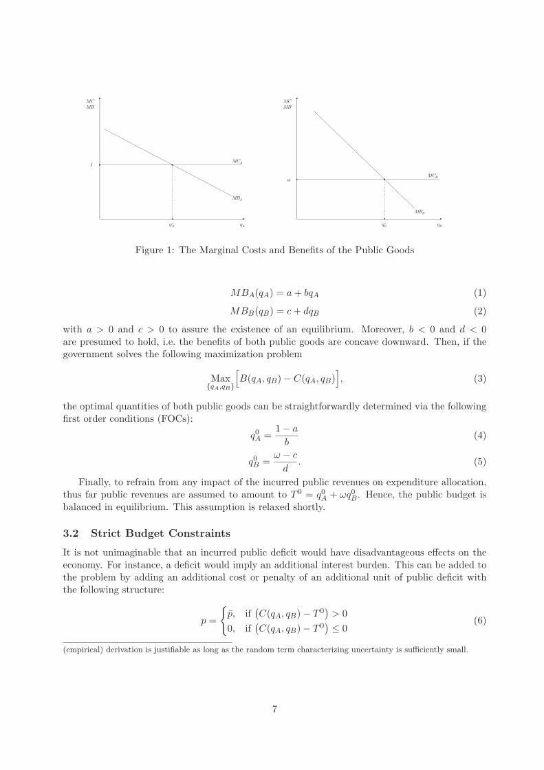
Consider a government whose expenditures are made up of the provision of multiple public goods.In the setup presented below the public goods are labeled i, with i ∈ {A,B}. Consequently, thequantities of both services provided by the government are denoted as qA and qB, respectively.Both goods have different short run marginal benefit or demand curves (MBi), derived from thegeneral benefit curve B(qA, qB). Yet, for simplicity, assume that the marginal cost of provisionfor public good A is standardized at 1, i.e. MCA = 1. Let the marginal cost of good B beproportional to this by factor ω: MCB = ω. Hence, total costs are the sum of public goodsprovided: C(qA, qB) = qA+ωqB. This assumption will be relaxed later. Furthermore, if quantitiesare such that for a price of 1 and ω respectively the optimal supply is {q0A, q0B}, the public fundsallocated to both public goods can be illustrated as in figure 1.

To enable comparison of this basic benchmark to later cases, assume the following general,linear marginal benefit functions:7

6The underlying theoretical framework is the most closely related to the literature using dynamic equilibriummodels to examine the effect of uncertain taxation (e.g. Bizer and Judd, 1989), though the focus being on publicexpenditures instead of fiscal revenues.

7One could see such general linear marginal functions as a second-order Taylor approximation of the actual totalbenefit and cost functions (see e.g. Weitzman, 1974). In case of uncertainty, as illustrated in sections 5 and 6, such

6

MCMB

qA

1

MBA

MCA

qA°

MCMB

qB

ω

qB

MCB

MBB

°

Figure 1: The Marginal Costs and Benefits of the Public Goods

MBA(qA) = a+ bqA (1)

MBB(qB) = c+ dqB (2)

with a > 0 and c > 0 to assure the existence of an equilibrium. Moreover, b < 0 and d < 0are presumed to hold, i.e. the benefits of both public goods are concave downward. Then, if thegovernment solves the following maximization problem

Max{qA,qB}

[B(qA, qB)− C(qA, qB)

], (3)

the optimal quantities of both public goods can be straightforwardly determined via the followingfirst order conditions (FOCs):

q0A =1− a

b(4)

q0B =ω − c

d. (5)

Finally, to refrain from any impact of the incurred public revenues on expenditure allocation,thus far public revenues are assumed to amount to T 0 = q0A + ωq0B. Hence, the public budget isbalanced in equilibrium. This assumption is relaxed shortly.

3.2 Strict Budget Constraints

It is not unimaginable that an incurred public deficit would have disadvantageous effects on theeconomy. For instance, a deficit would imply an additional interest burden. This can be added tothe problem by adding an additional cost or penalty of an additional unit of public deficit withthe following structure:

p =

{p, if

(C(qA, qB)− T 0

)> 0

0, if(C(qA, qB)− T 0

) ≤ 0(6)

(empirical) derivation is justifiable as long as the random term characterizing uncertainty is sufficiently small.

7

where p > 0. As a result, the government will solve the following optimization problem (insteadof (3)):8

Max{qA,qB}

[B(qA, qB)− C(qA, qB)− p

(C(qA, qB)− T 0

)]. (7)

Inserting the respective costs of public expenditures in (7) and simplifying yields Max{qA,qB}

[B(qA, qB)+

pT 0 − (1 + p)(qA + ωqB)].9 This results in the following first order conditions:

q00A =(1 + p)− a

b(8)

q00B =(1 + p)ω − c

d(9)

with p’s structure defined as in (6).As illustrated in figure 2, the optimization taking into account the stricter constraint does

however not change the allocation of public goods as long as revenues are known ex ante to be T 0.As a result, q00A = q0A and q00B = q0B will still hold and the budget is balanced too.

MCMB

qA

1

MBA

MCA+p

qA°

MCMB

qB

ω

qB

MBB

°

MCB+ωp

Figure 2: The Marginal Costs and Benefits of the Public Goods in case of Costly Deficits

In case p = p holds for(C(qA, qB)−T 0

) ≤ 0 as well, lower provisions of both public goods willbe chosen by the government and a budget surplus results (as illustrated in appendix A.2). Thisis a logical result as the symmetry of p would, in addition to the economic cost of a deficit, implya gain for the government via an additional fee in case of austere budgetary behavior.

4 Introductory Examples of Uncertainty

Given that preferences for public goods are rather stable, the most credible way to add expenditureuncertainty to the model is via their cost of provision. An uncertain cost might for instance resultfrom shocks to wages, shocks to energy prices (e.g. the oil price) or a very harsh winter.

8The strict budget constraint implemented is thus nothing more than a balanced budget constraint with thecorresponding Lagrangian multiplier specified as a conditional market penalty p.

9Similarly, equations (7) and (6) can be combined to result in the following maximization problem

Max{qA,qB}

[B(qA, qB) − (qA + ωqB) − p.max

(qA + ωqB − T 0, 0

)]resulting in the same allocation, as shown in ap-

pendix A.1.

8

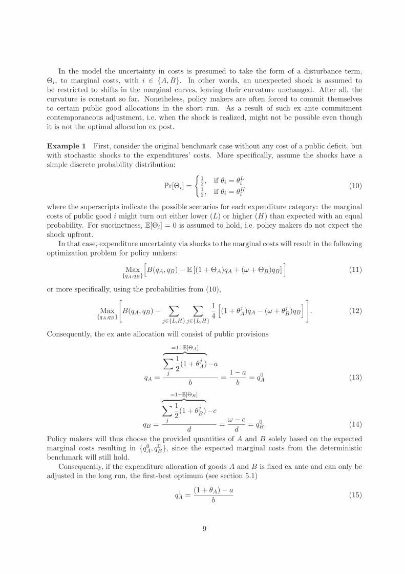
In the model the uncertainty in costs is presumed to take the form of a disturbance term,Θi, to marginal costs, with i ∈ {A,B}. In other words, an unexpected shock is assumed tobe restricted to shifts in the marginal curves, leaving their curvature unchanged. After all, thecurvature is constant so far. Nonetheless, policy makers are often forced to commit themselvesto certain public good allocations in the short run. As a result of such ex ante commitmentcontemporaneous adjustment, i.e. when the shock is realized, might not be possible even thoughit is not the optimal allocation ex post.

Example 1 First, consider the original benchmark case without any cost of a public deficit, butwith stochastic shocks to the expenditures’ costs. More specifically, assume the shocks have asimple discrete probability distribution:

Pr[Θi] =

{12 , if θi = θLi12 , if θi = θHi

(10)

where the superscripts indicate the possible scenarios for each expenditure category: the marginalcosts of public good i might turn out either lower (L) or higher (H) than expected with an equalprobability. For succinctness, E[Θi] = 0 is assumed to hold, i.e. policy makers do not expect theshock upfront.

In that case, expenditure uncertainty via shocks to the marginal costs will result in the followingoptimization problem for policy makers:

Max{qA,qB}

[B(qA, qB)− E [(1 + ΘA)qA + (ω +ΘB)qB]

](11)

or more specifically, using the probabilities from (10),

Max{qA,qB}

[B(qA, qB)−

∑j∈{L,H}

∑j∈{L,H}

1

4

[(1 + θjA)qA − (ω + θjB)qB

] ]. (12)

Consequently, the ex ante allocation will consist of public provisions

qA =

=1+E[ΘA]︷ ︸︸ ︷∑j

1

2(1 + θjA)−a

b=

1− a

b= q0A (13)

qB =

=1+E[ΘB ]︷ ︸︸ ︷∑j

1

2(1 + θjB)−c

d=

ω − c

d= q0B. (14)

Policy makers will thus choose the provided quantities of A and B solely based on the expectedmarginal costs resulting in {q0A, q0B}, since the expected marginal costs from the deterministicbenchmark will still hold.

Consequently, if the expenditure allocation of goods A and B is fixed ex ante and can only beadjusted in the long run, the first-best optimum (see section 5.1)

q1A =(1 + θA)− a

b(15)

9

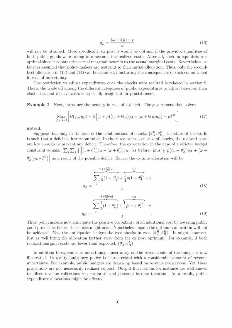
q1B =(ω + θB)− c

d(16)

will not be attained. More specifically, ex post it would be optimal if the provided quantities ofboth public goods were taking into account the realized costs. After all, such an equilibrium isoptimal since it equates the actual marginal benefits to the actual marginal costs. Nevertheless, sofar it is assumed that policy makers are restraint to their initial allocation. Thus, only the second-best allocation in (13) and (14) can be attained, illustrating the consequences of such commitmentin case of uncertainty.

The restriction to adjust expenditures once the shocks were realized is relaxed in section 9.There, the trade off among the different categories of public expenditures to adjust based on theirelasticities and relative costs is especially insightful for practitioners.

Example 2 Next, introduce the penalty in case of a deficit. The government then solves

Max{qA,qB}

[B(qA, qB)− E

[(1 + p)

((1 + ΘA)qA + (ω +ΘB)qB

)− pT 0]]

(17)

instead.Suppose that only in the case of the combinations of shocks {θHA , θHB } the state of the world

is such that a deficit is insurmountable. In the three other scenarios of shocks, the realized costsare low enough to prevent any deficit. Therefore, the expectation in the case of a stricter budget

constraint equals:∑

j

∑j14

[(1 + θjA)qA − (ω + θjB)qB

]as before, plus 1

4

[p((1 + θHA )qA + (ω +

θHB )qB−T 0)]

as a result of the possible deficit. Hence, the ex ante allocation will be

qA =

=1+E[θA]︷ ︸︸ ︷∑j

1

2(1 + θjA)+

>0︷ ︸︸ ︷1

4p(1 + θHA )−a

b(18)

qB =

=1+E[θB ]︷ ︸︸ ︷∑j

1

2(1 + θjB)+

>0︷ ︸︸ ︷1

4p(ω + θHB )−c

d. (19)

Thus, policymakers now anticipate the positive probability of an additional cost by lowering publicgood provisions before the shocks might arise. Nonetheless, again the optimum allocation will notbe achieved. Yet, the anticipation hedges the cost shocks in case {θHA , θHB }. It might, however,just as well bring the allocation farther away from the ex post optimum. For example, if bothrealized marginal costs are lower than expected, {θLA, θLB}.

In addition to expenditure uncertainty, uncertainty on the revenue side of the budget is nowillustrated. In reality budgetary policy is characterized with a considerable amount of revenueuncertainty. For example, public budgets are drawn up based on revenue projections. Yet, theseprojections are not necessarily realized ex post. Output fluctuations for instance are well knownto affect revenue collections via corporate and personal income taxation. As a result, publicexpenditure allocations might be affected.

10

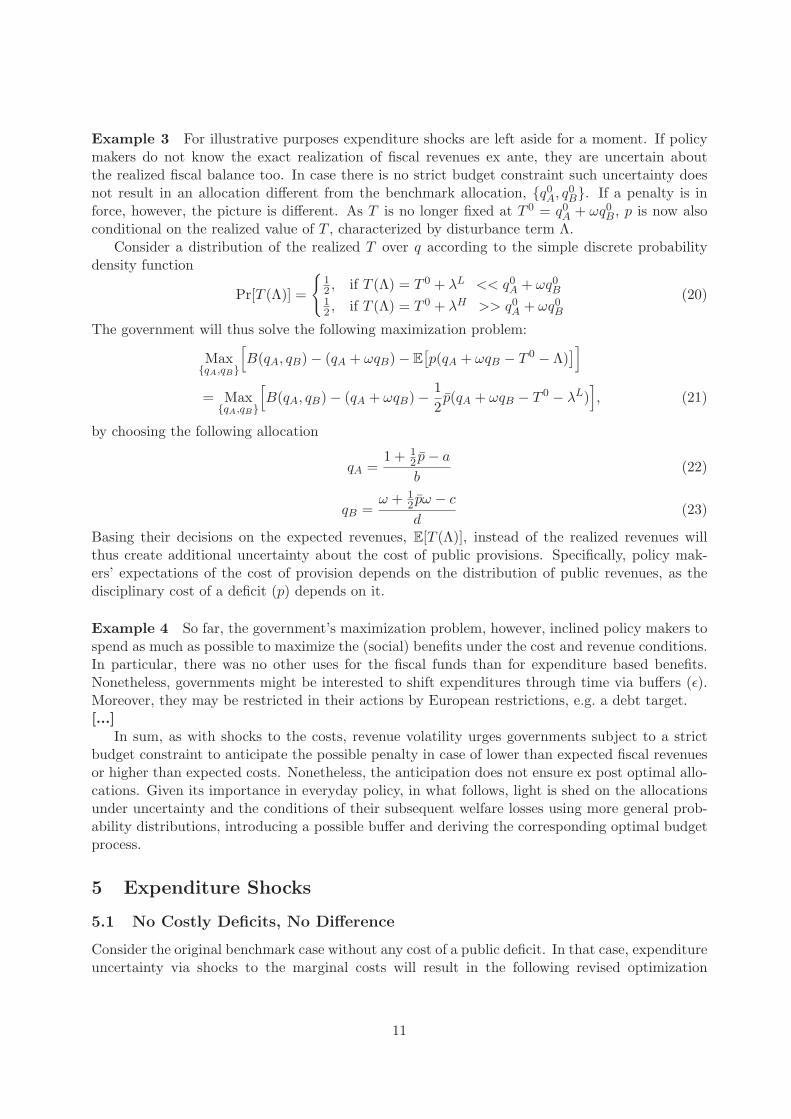
Example 3 For illustrative purposes expenditure shocks are left aside for a moment. If policymakers do not know the exact realization of fiscal revenues ex ante, they are uncertain aboutthe realized fiscal balance too. In case there is no strict budget constraint such uncertainty doesnot result in an allocation different from the benchmark allocation, {q0A, q0B}. If a penalty is inforce, however, the picture is different. As T is no longer fixed at T 0 = q0A + ωq0B, p is now alsoconditional on the realized value of T , characterized by disturbance term Λ.

Consider a distribution of the realized T over q according to the simple discrete probabilitydensity function

Pr[T (Λ)] =

{12 , if T (Λ) = T 0 + λL << q0A + ωq0B12 , if T (Λ) = T 0 + λH >> q0A + ωq0B

(20)

The government will thus solve the following maximization problem:

Max{qA,qB}

[B(qA, qB)− (qA + ωqB)− E

[p(qA + ωqB − T 0 − Λ)

]]= Max

{qA,qB}

[B(qA, qB)− (qA + ωqB)− 1

2p(qA + ωqB − T 0 − λL)

], (21)

by choosing the following allocation

qA =1 + 1

2 p− a

b(22)

qB =ω + 1

2 pω − c

d(23)

Basing their decisions on the expected revenues, E[T (Λ)], instead of the realized revenues willthus create additional uncertainty about the cost of public provisions. Specifically, policy mak-ers’ expectations of the cost of provision depends on the distribution of public revenues, as thedisciplinary cost of a deficit (p) depends on it.

Example 4 So far, the government’s maximization problem, however, inclined policy makers tospend as much as possible to maximize the (social) benefits under the cost and revenue conditions.In particular, there was no other uses for the fiscal funds than for expenditure based benefits.Nonetheless, governments might be interested to shift expenditures through time via buffers (ε).Moreover, they may be restricted in their actions by European restrictions, e.g. a debt target.[...]

In sum, as with shocks to the costs, revenue volatility urges governments subject to a strictbudget constraint to anticipate the possible penalty in case of lower than expected fiscal revenuesor higher than expected costs. Nonetheless, the anticipation does not ensure ex post optimal allo-cations. Given its importance in everyday policy, in what follows, light is shed on the allocationsunder uncertainty and the conditions of their subsequent welfare losses using more general prob-ability distributions, introducing a possible buffer and deriving the corresponding optimal budgetprocess.

5 Expenditure Shocks

5.1 No Costly Deficits, No Difference

Consider the original benchmark case without any cost of a public deficit. In that case, expenditureuncertainty via shocks to the marginal costs will result in the following revised optimization

11

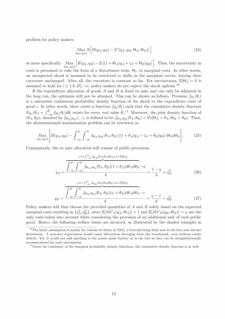
problem for policy makers:

Max{qA,qB}

E

[B(qA, qB)− [C(qA, qB,ΘA,ΘB)]

](24)

or more specifically: Max{qA,qB}

[B(qA, qB)−E [(1 + ΘA)qA + (ω +ΘB)qB]

]. Thus, the uncertainty in

costs is presumed to take the form of a disturbance term, Θi, to marginal costs. In other words,an unexpected shock is assumed to be restricted to shifts in the marginal curves, leaving theircurvature unchanged. After all, the curvature is constant so far. For succinctness, E[Θi] = 0 isassumed to hold for i ∈ {A,B}, i.e. policy makers do not expect the shock upfront.10

If the expenditure allocation of goods A and B is fixed ex ante and can only be adjusted inthe long run, the optimum will not be attained. This can be shown as follows. Presume fΘi(θi)is a univariate continuous probability density function of the shock to the expenditure costs ofgood i. In other words, there exists a function fΘi(θi) such that the cumulative density function

FΘi(θi) =∫ θi−∞ fΘi(θi)dθi exists for every real value θi.

11 Moreover, the joint density function of(θA, θB), denoted by fΘA,ΘB

(·, ·), is defined to be fΘA,ΘB(θA, θB) = Pr[ΘA = θA,ΘB = θB]. Then,

the aforementioned maximization problem can be rewritten as

Max{qA,qB}

[B(qA, qB)−

∫ ∞

−∞

∫ ∞

−∞fΘA,ΘB

(θA, θB) [(1 + θA)qA − (ω + θB)qB] dθAdθB

]. (25)

Consequently, the ex ante allocation will consist of public provisions

qA =

=1+∫∞−∞ fΘA

(θA)θAdθA=1+E[θA]︷ ︸︸ ︷∫ ∞

−∞

∫ ∞

−∞fΘA,ΘB

(θA, θB)(1 + θA)dθAdθB −a

b=

1− a

b= q0A (26)

qB =

=ω+∫∞−∞ fΘB

(θB)θBdθB=ω+E[θB ]︷ ︸︸ ︷∫ ∞

−∞

∫ ∞

−∞fΘA,ΘB

(θA, θB)(ω + θB)dθAdθB −c

d=

ω − c

d= q0B. (27)

Policy makers will thus choose the provided quantities of A and B solely based on the expectedmarginal costs resulting in {q0A, q0B}, since E[MCA(qA,ΘA)] = 1 and E[MCB(qB,ΘB)] = ω are theonly costs taken into account when considering the provision of an additional unit of each publicgood. Hence, the following welfare losses are incurred, as illustrated by the shaded triangles in

10The latter assumption is mainly for reasons of clarity as E[Θi] �= 0 would bring little new to the fore and obscurederivations. A non-zero expectation would cause allocations diverging from the benchmark, even without costlydeficits. Yet, it would not add anything to the points made further on in the text as they can be straightforwardlyaccommodated for such anticipation.

11Given the continuity of the marginal probability density functions, the cumulative density function is as well.

12

figure 3:

LgA =

1

2

(MCA(q

0A, θA)− E[MCA(q

0A,ΘA)]

)(q0A − q1A

)= −θ2A

2b(28)

LgB =

1

2

(MCB(q

0B, θB)− E[MCB(q

0B,ΘB)]

)(q0B − q1B

)= −θ2B

2d, (29)

where the ex post optimum quantities, q1i , are comprised by the following allocation:

q1A =(1 + θA)− a

b(30)

q1B =(ω + θB)− c

d. (31)

Whether these provisions are smaller or larger than {q0A, q0B} depends on whether the shocks to

marginal costs θi turn out to be positive or negative, respectively. More specifically,∂q1i∂θi

< 0 holdsfor both expenditure categories. Thus, if actual marginal costs are higher than expected (θi > 0),the optimum allocation would entail lower provision of public goods than those chosen based onthe expected costs, and vice versa.

MCMB

1

MBA

E[MCA]

MCA

q1A qAqA°

1+θA

MCMB

qB

ω

qB

MBB

°

MCB

E[MCB]

ω(1+θB)

q1B

Figure 3: The Marginal Costs and Benefits of the Public Goods in case of Cost Uncertainty

Despite the expected shocks being zero, comparison with the optimal allocation in the deter-ministic benchmark reveals a first channel of welfare losses under the condition of no contem-poraneous adjustment of public good allocations once the shocks have occurred. This can besummarized by proposition 1, from which it is clear that not only the size of the shocks but alsothe slopes of the marginal benefit curves (i.e. the elasticity of the public goods) is an importantdeterminant of the losses.

Proposition 1. (Expenditure Uncertainty I) Let MBi(qi) be a downward sloping marginal benefitfunction and let MCi(Θi) be a constant stochastic marginal cost function, with i ∈ {A,B} andshocks θi ∼ FΘi(0, σ

2i ). Then, the government’s inability to adjust the allocation {q0A, q0B} to

13

expenditure shocks in the short run, yields deadweight losses amounting to LgA = − θ2A

2b and LgB =

− θ2B2d , respectively.

5.2 Costly Deficits, Anticipated Uncertainty

Next, consider the case of a shock on the expenditure side taking into account the cost of a possibledeficit. The government then solves

Max{qA,qB}

E

[B(qA, qB)− C(qA, qB,ΘA,ΘB)− p(C(qA, qB,ΘA,ΘB)− T 0)

]Or similarly Max

{qA,qB}

[B(qA, qB)− E

[(1 + p)

((1 + ΘA)qA + (ω +ΘB)qB

)− pT 0]]

(32)

with p taking taking on the conditional values as specified in (6) adjusted for cost uncertainty:

p =

{p, if

(C(qA, qB, θA, θB)− T 0

)> 0

0, if(C(qA, qB, θA, θB)− T 0

) ≤ 0(33)

As in section 5.1, solving this problem for the ex ante public good allocation requires the speci-fication of a distribution for the shocks. Nevertheless, the asymmetric structure of p will have adistinct impact on ex ante behavior as policy makers will choose allocations conditional on theprobability that shocks may cause a deficit and thus a penalty.

5.2.1 Homogeneous Shocks

As a means of illustration, first consider the case where both shocks to the marginal costs ofboth public goods are the same (θA = θB = θ), with a distribution fΘ(θ) for such a shock. Asillustrated below, the presence of an asymmetric factor comprising the adverse economic effectsof public deficit results in an ex ante commitment different from the benchmark case without theeconomic cost of a deficit.

In particular, even with T 0 fixed policy makers do not know ex ante at which expenditureallocations an additional cost will be incurred due to a deficit. After all, they do not know theexact marginal cost due to the possible disturbance. Yet, this disturbance will affect the economicpenalty incurred due to fiscal profligacy and the ex post optimality of their choice. Specifically,

solving the expectation E

[(1+p)

((1+ΘA)qA+(ω+ΘB)qB −pT 0

)]in (32) gives the integral over

Θ of all occurrences of the shock, Pr[θ] · [(1 + θ)qA + (ω + θ)qB], plus the integral over Θ of the

occurrences of the shock for which there is a deficit, Pr[θ] · [p((1 + θ)qA + (ω + θ)qB − T 0)].

14

In particular, by means of probability density function fΘ(θ), policy makers solve:12

Max{qA,qB}

[B(qA, qB)−

∫ ∞

−∞fΘ(θ) [(1 + θ)qA + (ω + θ)qB] dθ

−∫ ∞

−∞fΘ(θ)

[p ·max

((1 + θ)qA + (ω + θ)qB − T 0, 0

)]dθ

](34)

= Max{qA,qB}

[B(qA, qB)−

∫ ∞

−∞fΘ(θ) [(1 + θ)qA + (ω + θ)qB] dθ

−∫ ∞

−∞fΘ(θ)

1

2p((1 + θ)qA + (ω + θ)qB − T 0 +

∣∣(1 + θ)qA + (ω + θ)qB − T 0∣∣ )︸ ︷︷ ︸

= 0, if((1 + θ)qA + (ω + θ)qB − T 0

) ≤ 0

> 0, if((1 + θ)qA + (ω + θ)qB − T 0

)> 0

dθ

].

Consequently, the ex ante allocation is

qA =1

b

(1 +

∫ ∞

−∞fΘ(θ)θdθ︸ ︷︷ ︸

=E[Θ]=0

+

∫ ∞

−∞fΘ(θ)

1

2p (1 + θ)

(1 +

(1 + θ)qA + (ω + θ)qB − T 0

|(1 + θ)qA + (ω + θ)qB − T 0|)

︸ ︷︷ ︸= 0, if

((1 + θ)qA + (ω + θ)qB − T 0

) ≤ 0

> 0, if((1 + θ)qA + (ω + θ)qB − T 0

)> 0 and θ > −1

dθ − a

)

=1 +

∫∞−∞ fΘ(θ)

12 p(1 + θ)

(1 + (1+θ)qA+(ω+θ)qB−T 0

|(1+θ)qA+(ω+θ)qB−T 0|)dθ − a

b(35)

qB =1

d

(ω +

∫ ∞

−∞fΘ(θ)θdθ︸ ︷︷ ︸

=E[Θ]=0

+

∫ ∞

−∞fΘ(θ)

1

2p (ω + θ)

(1 +

(1 + θ)qA + (ω + θ)qB − T 0

|(1 + θ)qA + (ω + θ)qB − T 0|)

︸ ︷︷ ︸= 0, if

((1 + θ)qA + (ω + θ)qB − T 0

) ≤ 0

> 0, if((1 + θ)qA + (ω + θ)qB − T 0

)> 0 and θ > −1

dθ − c

)

=ω +

∫∞−∞ fΘ(θ)

12 p(ω + θ)

(1 + (1+θ)qA+(ω+θ)qB−T 0

|(1+θ)qA+(ω+θ)qB−T 0|)dθ − c

d. (36)

Therefore, as long as the probabilities of unreasonably large downward shocks to public goods’prices are small, there will be anticipation via lower provisions of public goods.13 14

12Distinguishing the realizations of the shock for which there will be a deficit is the result of an iterative processby policy makers. In particular, the positive expectation of a penalty

∫∞0

fΘ(θ)[p((1+θ)qA+(ω+θ)qB−T 0

)]dθ will

cause the government to anticipate by lowering public provisions. Thereby, creating a lower probability of runninga deficit and thus incurring a penalty. This will, in its turn, lower the anticipation and thus increase the probabilityof penalty. The process continues until an equilibrium allocation has been reached.

13An alternative derivation of this result is presented in appendix A.4. Nonetheless, the method used in the maintext is less burdensome once the assumption of homogeneous shocks is dropped.

14The public administration’s stance with respect to risk nonetheless matters for the degree of anticipation (seee.g. Adar and Griffin (1976)). In particular, a risk neutral government will base its decisions on its expected marginalcosts (incl. possible penalty), while a risk averse policy maker will pass judgment in a more behavioral manner (e.g.based on a utility function quantifying its valuation of risk). Nevertheless, anticipatory behavior is observed in caseof risk neutrality as well.

15

Proposition 2. (Expenditure Uncertainty II) Let MBi(qi) be a downward sloping marginal benefitfunction and let MCi(Θ) be a constant stochastic marginal cost function, with i ∈ {A,B}. Then,an asymmetric cost structure for the public deficit p > 0 and shocks θ ∼ FΘ(0, σ

2) with smallenough probability fΘ(θ) for unreasonably large downward shocks (i.e. Θ < −1), yield short runpublic provisions qA < q00A and qB < q00B under expenditure uncertainty.

In addition to the cost shocks, the incurred welfare losses are now also depending on the costp of too high expenditures for given revenues (i.e. fiscal indiscipline). In particular, the ex postoptimal allocation would have been:

q11A =(1 + p)(1 + θ)− α

β(37)

q11B =(1 + p)(ω + θ)− χ

δ(38)

Therefore, the incurred deadweight losses are

LgA =

1

2

(MCA(qA, θ) + p(1 + θ)− E[MCA(qA,Θ)] (39)

+

∫ ∞

−∞fΘ(θ)

1

2p(1 + θ)

(1 +

(1 + θ)qA + (ω + θ)qB − T 0

|(1 + θ)qA + (ω + θ)qB − T 0|)dθ

)(qA − q11A

)

=

⎧⎪⎪⎨⎪⎪⎩−(θ+p(1+θ)−∫∞

−∞ fΘ(θ) 12p(1+θ)

(1+

(1+θ)qA+(ω+θ)qB−T0

|(1+θ)qA+(ω+θ)qB−T0|)dθ)2

2β , if(C(qA, qB, θ)− T 0

)> 0

−(θ−∫∞

−∞ fΘ(θ) 12p(1+θ)

(1+

(1+θ)qA+(ω+θ)qB−T0

|(1+θ)qA+(ω+θ)qB−T0|)dθ)2

2β , if(C(qA, qB, θ)− T 0

) ≤ 0

LgB =

1

2

(MCB(qB, θ) + p(ω + θ)− E[MCB(qB,Θ)] (40)∫ ∞

−∞fΘ(θ)

1

2p(ω + θ)

(1 +

(1 + θ)qA + (ω + θ)qB − T 0

|(1 + θ)qA + (ω + θ)qB − T 0|)dθ

)(qB − q11B

)

=

⎧⎪⎪⎨⎪⎪⎩−(θ+p(ω+θ)−∫∞

−∞ fΘ(θ) 12p(ω+θ)

(1+

(1+θ)qA+(ω+θ)qB−T0

|(1+θ)qA+(ω+θ)qB−T0|)dθ)2

2δ , if(C(qA, qB, θ)− T 0

)> 0

−(θ−∫∞

−∞ fΘ(θ) 12p(ω+θ)

(1+

(1+θ)qA+(ω+θ)qB−T0

|(1+θ)qA+(ω+θ)qB−T0|)dθ)2

2δ , if(C(qA, qB, θ)− T 0

) ≤ 0

Even though the penalty fines - thus, not the losses - as a result of the (expected) shock onthe expenditure side will be anticipated by ex ante allocations different from the deterministicbenchmark as a result of the asymmetrical cost structure, the first channel of welfare losses fromsection 5.1 persists. Moreover, in addition to the distortions caused by the predetermination ofthe ex ante quantities of public provision, a disciplinary market mechanism may create additionaldistortions.15 In particular, the anticipation may just as well prove to have been unnecessary.

The realized deficit and cost of the ex ante allocation depend on the realized shocks. Assummarized by proposition 2, policy makers are found to reduce their provisions to anticipate the

15The result that the additional cost due to a public deficit matters for the welfare losses still holds in case of’perfect’ anticipation of the penalty due to a symmetric p. After all, the anticipation codetermines the deviation ofthe ex ante allocation from the optimum determined by the shocks, as illustrated in appendix A.3.

16

expected positive penalty as a result of the asymmetric cost structure. Therefore, the disciplinarycost brings short run allocations closer to the optimum in case higher than benchmark marginalcosts are realized. Nonetheless, if actual marginal costs are lower, discipline is still in force aspublic expenditures are capped at the benchmark due to the resulting cost structure.

Lemma 1. (Retaliation for Fiscal Indiscipline via Cost Shocks) With a cost for fiscal indisciplineas specified in equation (6) revenue volatility creates one-sided anticipatory behavior by reducingpublic goods’ provisions to {qA, qB}. Hence, retaliation for fiscal indiscipline both hedges againstthe impact of higher public expenditure costs and disciplines in case marginal costs fall belowexpectations.

Consequently, the markets’ retaliation for fiscal indiscipline via the cost of a public deficit spurspolicy makers to hedge against disadvantageous shocks on the expenditure side, while maintainingdiscipline in advantageous times. The conditions under which such discipline is harmful for welfareare explored further in section 5.2.2.

5.2.2 Heterogeneous Shocks

Now, again consider the objective function (32) with heterogeneous shocks and the general con-tinuous probability density function fΘi(θi) for the shocks to expenditure costs. Policy mak-ers thus choose quantities qA and qB by balancing benefits against expected costs, i.e. the in-tegral over vector (ΘA,ΘB) of Pr[θA ∩ θB] ·

[(1 + θA)qA + (ω + θB)qB

]plus the integral over

Pr[θA ∩ θB] ·[p((1 + θA)qA + (ω + θB)qB − T 0

)]in case of a deficit.

The corresponding maximization problem equals:

Max{qA,qB}

[B(qA, qB)−

∫ ∞

−∞

∫ ∞

−∞fΘA,ΘB

(θA, θB) [(1 + θA)qA − (ω + θB)qB] dθAdθB

−∫ ∞

−∞

∫ ∞

−∞fΘA,ΘB

(θA, θB)[p ·max

((1 + θA)qA + (ω + θB)qB − T 0, 0

)]dθAdθB

].

with, as in 5.2.1, the incurred penalty being a function of the realizations of both shocks and theallocation itself. Therefore, the ex ante allocation of public goods chosen by the government is:

qA =1

b

[1 +

∫ ∞

−∞

∫ ∞

−∞fΘA,ΘB

(θA, θB)θAdθAdθB︸ ︷︷ ︸=∫∞−∞ fΘA

(θA)θAdθA=E[ΘA]=0

+

∫ ∞

−∞

∫ ∞

−∞fΘA,ΘB

(θA, θB)1

2p (1 + θA)

(1 +

(1 + θA)qA + (ω + θB)qB − T 0

|(1 + θA)qA + (ω + θB)qB − T 0|)

︸ ︷︷ ︸= 0, if

((1 + θA)qA + (ω + θB)qB − T 0

) ≤ 0

> 0, if((1 + θA)qA + (ω + θB)qB − T 0

)> 0 and θA > −1

dθAdθB − a

]

=1 +

∫∞−∞

∫∞−∞ fΘA,ΘB

(θA, θB)12 p(1 + θA)

(1 + (1+θA)qA+(ω+θB)qB−T 0

|(1+θA)qA+(ω+θB)qB−T 0|)dθAdθB − a

b(41)

17

qB =1

d

[ω +

∫ ∞

−∞

∫ ∞

−∞fΘA,ΘB

(θA, θB)θBdθAdθB︸ ︷︷ ︸=∫∞−∞ fΘB

(θB)θBdθB=E[ΘB ]=0

+

∫ ∞

−∞

∫ ∞

−∞fΘA,ΘB

(θA, θB)1

2p (ω + θB)

(1 +

(1 + θA)qA + (ω + θB)qB − T 0

|(1 + θA)qA + (ω + θB)qB − T 0|)

︸ ︷︷ ︸= 0, if

((1 + θA)qA + (ω + θB)qB − T 0

) ≤ 0

> 0, if((1 + θA)qA + (ω + θB)qB − T 0

)> 0 and θB > −ω

dθAdθB − c

]

=ω +

∫∞−∞

∫∞−∞ fΘA,ΘB

(θA, θB)12 p(ω + θB)

(1 + (1+θA)qA+(ω+θB)qB−T 0

|(1+θA)qA+(ω+θB)qB−T 0|)dθAdθB − c

d. (42)

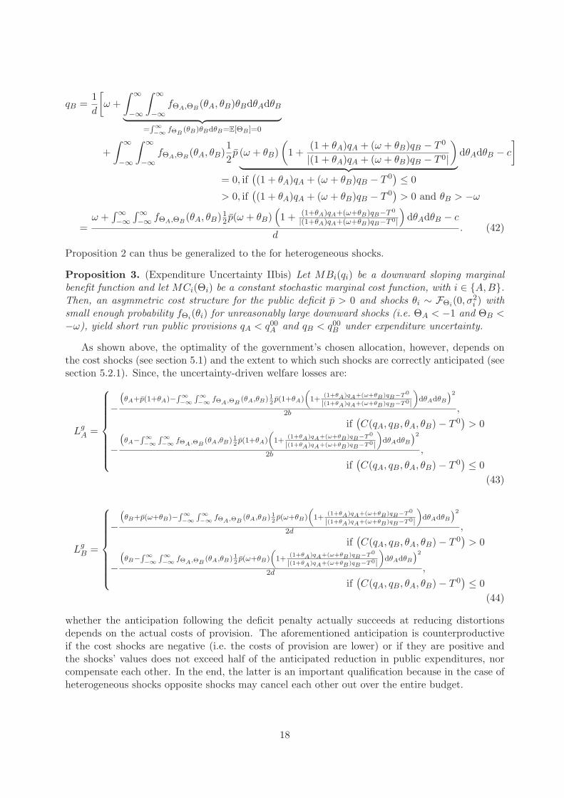
Proposition 2 can thus be generalized to the for heterogeneous shocks.

Proposition 3. (Expenditure Uncertainty IIbis) Let MBi(qi) be a downward sloping marginalbenefit function and let MCi(Θi) be a constant stochastic marginal cost function, with i ∈ {A,B}.Then, an asymmetric cost structure for the public deficit p > 0 and shocks θi ∼ FΘi(0, σ

2i ) with

small enough probability fΘi(θi) for unreasonably large downward shocks (i.e. ΘA < −1 and ΘB <−ω), yield short run public provisions qA < q00A and qB < q00B under expenditure uncertainty.

As shown above, the optimality of the government’s chosen allocation, however, depends onthe cost shocks (see section 5.1) and the extent to which such shocks are correctly anticipated (seesection 5.2.1). Since, the uncertainty-driven welfare losses are:

LgA =

⎧⎪⎪⎪⎪⎪⎪⎪⎨⎪⎪⎪⎪⎪⎪⎪⎩

−(θA+p(1+θA)−∫∞

−∞∫∞−∞ fΘA,ΘB

(θA,θB) 12p(1+θA)

(1+

(1+θA)qA+(ω+θB)qB−T0

|(1+θA)qA+(ω+θB)qB−T0|)dθAdθB

)22b ,

if(C(qA, qB, θA, θB)− T 0

)> 0

−(θA−∫∞

−∞∫∞−∞ fΘA,ΘB

(θA,θB) 12p(1+θA)

(1+

(1+θA)qA+(ω+θB)qB−T0

|(1+θA)qA+(ω+θB)qB−T0|)dθAdθB

)22b ,

if(C(qA, qB, θA, θB)− T 0

) ≤ 0

(43)

LgB =

⎧⎪⎪⎪⎪⎪⎪⎪⎨⎪⎪⎪⎪⎪⎪⎪⎩

−(θB+p(ω+θB)−∫∞

−∞∫∞−∞ fΘA,ΘB

(θA,θB) 12p(ω+θB)

(1+

(1+θA)qA+(ω+θB)qB−T0

|(1+θA)qA+(ω+θB)qB−T0|)dθAdθB

)22d ,

if(C(qA, qB, θA, θB)− T 0

)> 0

−(θB−∫∞

−∞∫∞−∞ fΘA,ΘB

(θA,θB) 12p(ω+θB)

(1+

(1+θA)qA+(ω+θB)qB−T0

|(1+θA)qA+(ω+θB)qB−T0|)dθAdθB

)22d ,

if(C(qA, qB, θA, θB)− T 0

) ≤ 0

(44)

whether the anticipation following the deficit penalty actually succeeds at reducing distortionsdepends on the actual costs of provision. The aforementioned anticipation is counterproductiveif the cost shocks are negative (i.e. the costs of provision are lower) or if they are positive andthe shocks’ values does not exceed half of the anticipated reduction in public expenditures, norcompensate each other. In the end, the latter is an important qualification because in the case ofheterogeneous shocks opposite shocks may cancel each other out over the entire budget.

18

Proposition 4. (Expenditure Uncertainty III) Let MBi(qi) be a downward sloping marginalbenefit function and let MCi(Θi) be a constant stochastic marginal cost function, with i ∈ {A,B}.Then, the anticipatorily lowered public provisions as a result of an asymmetric cost structure forthe public deficit p > 0 and shocks θi ∼ FΘi(0, σ

2i ), are counterproductive in hedging against

expenditure uncertainty if the shocks are negative or if they are positive and do not exceed half ofthe anticipated reduction in public expenditures.

[TBC]

6 Revenue Uncertainty

If policy makers do not know the exact realization of fiscal revenues ex ante, they are uncertainabout the realized fiscal balance too. In case there is no strict budget constraint such uncertaintydoes not result in an allocation different from {q0A, q0B} from section 5.1. If a penalty is in force,however, the picture is different. As T is no longer fixed at T 0 = q0A+ωq0B, p is now also conditionalon the realized value of T , characterized by disturbance term Λ:

p =

{p, if

(C(qA, qB)− T (λ)

)> 0

0, if(C(qA, qB)− T (λ)

) ≤ 0(45)

In particular, basing their decisions on the expected revenues, E[T (Λ)], instead of the realizedrevenues will create additional uncertainty about the cost of public provisions. Specifically, policymakers’ expectations of the cost of provision depends on the distribution of public revenues, asthe disciplinary cost of a deficit (p) depends on it.

Consider a distribution of Λ according to Λ ∼ FΛ(0, σ2t ) and a corresponding continuous

probability density function fΛ(λ). Hence, the distribution of the realized T (λ), i.e. T 0 + λ, overq according to probability density function fT

(T (λ)

), with T (Λ) ∼ FT (q

0A + ωq0B, σ

2t ). Hence, the

corresponding government’s maximization,

Max{qA,qB}

[B(qA, qB)− (qA + ωqB)− E

[p(qA + ωqB − T 0 − λ)

]]= Max

{qA,qB}

[B(qA, qB)− (qA + ωqB)− Pr[p = p|T (λ)] · p(qA + ωqB − T (λ)

)]= Max

{qA,qB}

[B(qA, qB)− (qA + ωqB)−

∫ C(qA,qB)

−∞p(qA + ωqB − T (λ)

)fT

(T (λ)

)dT

], (46)

will result in the following quantities:

q2A =

1 +

>0︷ ︸︸ ︷∫ qA+ωqB

−∞pfT

(T (λ)

)dT −a

b(47)

q2B =

ω +

>0︷ ︸︸ ︷∫ qA+ωqB

−∞pωfT

(T (λ)

)dT −c

d. (48)

19

Since the continuous probability density function is positive over its domain (i.e. fT(T (λ)

)> 0),

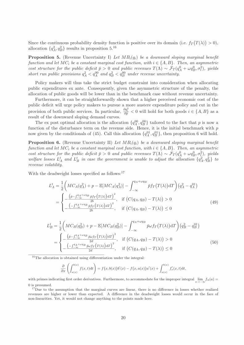
allocation {q2A, q2B} results in proposition 5.16

Proposition 5. (Revenue Uncertainty I) Let MBi(qi) be a downward sloping marginal benefitfunction and let MCi be a constant marginal cost function, with i ∈ {A,B}. Then, an asymmetriccost structure for the public deficit p > 0 and public revenues T (Λ) ∼ FT (q

0A + ωq0B, σ

2t ), yields

short run public provisions q2A < q00A and q2B < q00B under revenue uncertainty.

Policy makers will thus take the strict budget constraint into consideration when allocatingpublic expenditures ex ante. Consequently, given the asymmetric structure of the penalty, theallocation of public goods will be lower than in the benchmark case without revenue uncertainty.

Furthermore, it can be straightforwardly shown that a higher perceived economic cost of thepublic deficit will urge policy makers to pursue a more austere expenditure policy and cut in the

provision of both public services. In particular,∂q2i∂p < 0 will hold for both goods i ∈ {A,B} as a

result of the downward sloping demand curves.The ex post optimal allocation is the allocation {q00A , q00B } tailored to the fact that p is now a

function of the disturbance term on the revenue side. Hence, it is the initial benchmark with pnow given by the conditionals of (45). Call this allocation {q01A , q01B }, then proposition 6 will hold.

Proposition 6. (Revenue Uncertainty II) Let MBi(qi) be a downward sloping marginal benefitfunction and let MCi be a constant marginal cost function, with i ∈ {A,B}. Then, an asymmetriccost structure for the public deficit p > 0 and public revenues T (Λ) ∼ FT (q

0A + ωq0B, σ

2t ), yields

welfare losses LtA and Lt

B in case the government is unable to adjust the allocation {q2A, q2B} torevenue volatility.

With the deadweight losses specified as follows:17

LtA =

1

2

(MCA(q

2A) + p− E[MCA(q

2A)]−

∫ qA+ωqB

−∞pfT

(T (λ)

)dT

)(q2A − q01A

)

=

⎧⎪⎨⎪⎩−(p−∫ qA+ωqB

−∞ pfT

(T (λ)

)dT)2

2b , if(C(qA, qB)− T (λ)

)> 0

−(−∫ qA+ωqB

−∞ pfT

(T (λ)

)dT)2

2b , if(C(qA, qB)− T (λ)

) ≤ 0

(49)

LtB =

1

2

(MCB(q

2B) + p− E[MCB(q

2B)]−

∫ qA+ωqB

−∞pωfT

(T (λ)

)dT

)(q2B − q01B

)

=

⎧⎪⎨⎪⎩−(p−∫ qA+ωqB

−∞ pωfT

(T (λ)

)dT)2

2d , if(C(qA, qB)− T (λ)

)> 0

−(−∫ qA+ωqB

−∞ pωfT

(T (λ)

)dT)2

2d , if(C(qA, qB)− T (λ)

) ≤ 0

(50)

16The allocation is obtained using differentiation under the integral:

∂

∂x

(∫ b(x)

a(x)

f(x, t)dt

)= f

(x, b(x)

)b′(x)− f

(x, a(x)

)a′(x) +

∫ b(x)

a(x)

f ′x(x, t)dt,

with primes indicating first order derivatives. Furthermore, to accommodate for the improper integral lima→−∞

fΛ(a) =

0 is presumed.17Due to the assumption that the marginal curves are linear, there is no difference in losses whether realized

revenues are higher or lower than expected. A difference in the deadweight losses would occur in the face ofnon-linearities. Yet, it would not change anything to the points made here.

20

Obviously, the realized deficit and cost of the ex ante allocation depend on the realized revenues.Policy makers are found to reduce their provisions to anticipate the expected positive penalty as aresult of the asymmetric cost structure. Therefore, the disciplinary cost brings short run allocationscloser to the optimum in case lower than benchmark revenues are collected. Nonetheless, if actualrevenues are higher, discipline is still in force as public expenditures are capped at the benchmarkdue to the resulting cost structure. Consequently, the markets’ retaliation for fiscal indisciplinevia the cost of public expenditures spurs policy makers to hedge against disadvantageous revenueshocks, while maintaining discipline in advantageous times albeit possibly at the cost of lowerwelfare.

Lemma 2. (Retaliation for Fiscal Indiscipline via Revenue Volatility) With a cost for fiscal in-discipline as specified in equation (45) revenue volatility creates one-sided anticipatory behaviorby reducing public goods’ provisions to {q2A, q2B}. Hence, retaliation for fiscal indiscipline bothhedges against the impact of lower fiscal revenues and disciplines in case fiscal revenues exceedexpectations.

In brief, although an anticipatory reduction of the supply of public goods might hedge againstpart of the revenue uncertainty, a second channel of welfare losses due to revenue volatility willpersist. For example, fiscal revenues might just as well turn out to be lower than expected and aneven lower provision might have been preferable ex post. Hence, conclusions similar to those forexpenditure shocks apply.

7 Compounded Uncertainty

To further generalize the model and its findings, expenditure cost shocks and revenue volatility arenow considered in unison. Firstly, section 7.1 does this for two public good categories, as before.Secondly, section 7.2 extends the model from two to N different types of expenditure categories.

7.1 Full-fledged Model

To further generalize the model and its findings, expenditure cost shocks and revenue volatility arenow considered in unison. Combining the revenue volatility from section 6 with the heterogeneouscost shocks from section 5.2.2 results in a model with three stochastic random variables. Take thejoint probability density function of those three variables fΘA,ΘB ,Λ(θA, θB, λ) as given. Moreover,the budget is balanced or: λ = (1 + θA)qA + (ω + θB)qB − T 0. Then, defining

χ(qA, qB, θA, θB) ≡ (1 + θA)qA + (ω + θB)qB − T 0, (51)

the government solves the following maximization problem:

Max{qA,qB}

[B(qA, qB)−

∫ ∞

−∞

∫ ∞

−∞fΘA,ΘB

(θA, θB) [(1 + θA)qA − (ω + θB)qB] dθAdθB

−∫ ∞

χ(qA,qB ,θA,θB)

∫ ∞

−∞

∫ ∞

−∞fΘA,ΘB ,Λ(θA, θB, λ)

[p · ((1 + θA)qA + (ω + θB)qB − (T 0 + λ)

)]dθAdθBdλ

].

Consequently, the ex ante allocation of public goods chosen by the government again portray

21

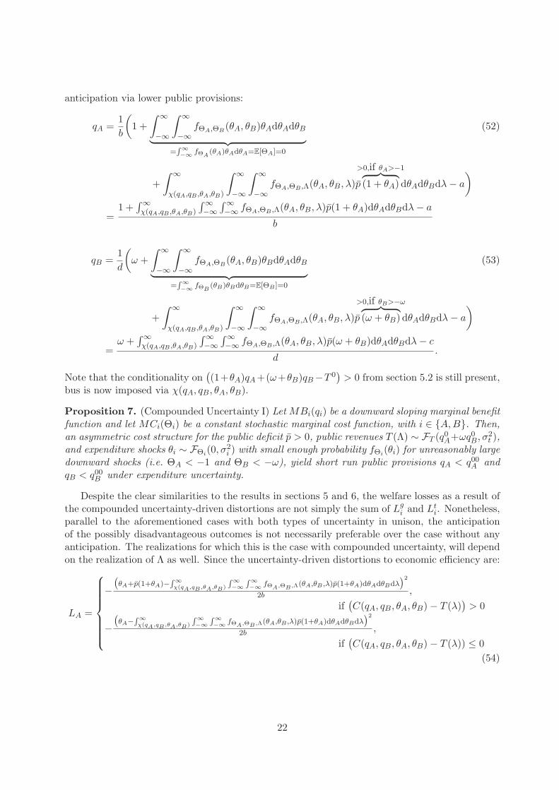
anticipation via lower public provisions:

qA =1

b

(1 +

∫ ∞

−∞

∫ ∞

−∞fΘA,ΘB

(θA, θB)θAdθAdθB︸ ︷︷ ︸=∫∞−∞ fΘA

(θA)θAdθA=E[ΘA]=0

(52)

+

∫ ∞

χ(qA,qB ,θA,θB)

∫ ∞

−∞

∫ ∞

−∞fΘA,ΘB ,Λ(θA, θB, λ)p

>0,if θA>−1︷ ︸︸ ︷(1 + θA) dθAdθBdλ− a

)

=1 +

∫∞χ(qA,qB ,θA,θB)

∫∞−∞

∫∞−∞ fΘA,ΘB ,Λ(θA, θB, λ)p(1 + θA)dθAdθBdλ− a

b

qB =1

d

(ω +

∫ ∞

−∞

∫ ∞

−∞fΘA,ΘB

(θA, θB)θBdθAdθB︸ ︷︷ ︸=∫∞−∞ fΘB

(θB)θBdθB=E[ΘB ]=0

(53)

+

∫ ∞

χ(qA,qB ,θA,θB)

∫ ∞

−∞

∫ ∞

−∞fΘA,ΘB ,Λ(θA, θB, λ)p

>0,if θB>−ω︷ ︸︸ ︷(ω + θB) dθAdθBdλ− a

)

=ω +

∫∞χ(qA,qB ,θA,θB)

∫∞−∞

∫∞−∞ fΘA,ΘB ,Λ(θA, θB, λ)p(ω + θB)dθAdθBdλ− c

d.

Note that the conditionality on((1+θA)qA+(ω+θB)qB−T 0

)> 0 from section 5.2 is still present,

bus is now imposed via χ(qA, qB, θA, θB).

Proposition 7. (Compounded Uncertainty I) Let MBi(qi) be a downward sloping marginal benefitfunction and let MCi(Θi) be a constant stochastic marginal cost function, with i ∈ {A,B}. Then,an asymmetric cost structure for the public deficit p > 0, public revenues T (Λ) ∼ FT (q

0A+ωq0B, σ

2t ),

and expenditure shocks θi ∼ FΘi(0, σ2i ) with small enough probability fΘi(θi) for unreasonably large

downward shocks (i.e. ΘA < −1 and ΘB < −ω), yield short run public provisions qA < q00A andqB < q00B under expenditure uncertainty.

Despite the clear similarities to the results in sections 5 and 6, the welfare losses as a result ofthe compounded uncertainty-driven distortions are not simply the sum of Lg

i and Lti. Nonetheless,

parallel to the aforementioned cases with both types of uncertainty in unison, the anticipationof the possibly disadvantageous outcomes is not necessarily preferable over the case without anyanticipation. The realizations for which this is the case with compounded uncertainty, will dependon the realization of Λ as well. Since the uncertainty-driven distortions to economic efficiency are:

LA =

⎧⎪⎪⎪⎪⎪⎪⎨⎪⎪⎪⎪⎪⎪⎩

−(θA+p(1+θA)−∫∞

χ(qA,qB,θA,θB)

∫∞−∞

∫∞−∞ fΘA,ΘB,Λ(θA,θB ,λ)p(1+θA)dθAdθBdλ

)22b ,

if(C(qA, qB, θA, θB)− T (λ)

)> 0

−(θA−∫∞

χ(qA,qB,θA,θB)

∫∞−∞

∫∞−∞ fΘA,ΘB,Λ(θA,θB ,λ)p(1+θA)dθAdθBdλ

)22b ,

if(C(qA, qB, θA, θB)− T (λ)) ≤ 0

(54)

22

LB =

⎧⎪⎪⎪⎪⎪⎪⎨⎪⎪⎪⎪⎪⎪⎩

−(θB+p(ω+θB)−∫∞

χ(qA,qB,θA,θB)

∫∞−∞

∫∞−∞ fΘA,ΘB,Λ(θA,θB ,λ)p(ω+θB)dθAdθBdλ

)22d ,

if(C(qA, qB, θA, θB)− T (λ)

)> 0

−(θB−∫∞

χ(qA,qB,θA,θB)

∫∞−∞

∫∞−∞ fΘA,ΘB,Λ(θA,θB ,λ)p(ω+θB)dθAdθBdλ

)22d ,

if(C(qA, qB, θA, θB)− T (λ)

) ≤ 0

(55)

shocks (θA, θB, λ) for which λ is greater or equal to (qi − q00i ) (i.e. the anticipation) and the costshock is (a) negative or (b) positive with the shock’s value not exceeding half of the anticipatedreduction in marginal benefits, will actually imply a range of realizations of expenditure costs andfiscal revenues for which anticipation is counterproductive. On the other hand, if λ is smaller than(qi − q00i ) this does not hold. Then, anticipation has an adverse effect in case the expenditureshock is smaller than λ minus half of the anticipated reduction in marginal benefits. The remarkwith respect to compensation between different expenditure categories within the overall budgetas a result of heterogeneous shocks, however, still holds (see section 5.2.2).

Proposition 8. (Compounded Uncertainty II) Let MBi(qi) be a downward sloping marginalbenefit function and let MCi(Θi) be a constant stochastic marginal cost function, with i ∈ {A,B}.Then, the anticipatorily lowered public provisions as a result of an asymmetric cost structure forthe public deficit p > 0, public revenues T (Λ) ∼ FT (q

0A+ωq0B, σ

2t ), and shocks θi ∼ FΘi(0, σ

2i ), are

counterproductive in hedging against expenditure uncertainty if:

a. λ ≥ (qi − q00i ) and the shock θi is either negative or positive but does not exceed half of theanticipated reduction in marginal benefits or;

b. λ < (qi − q00i ) and the shock θi is smaller than λ minus half of the anticipated reduction inmarginal benefits.

[TBC]

7.2 N-Vector Model

[TBC]

8 Buffer Provisions for the Future

So far, the government’s maximization problem, however, inclined policy makers to spend as muchas possible to maximize the (social) benefits under the cost and revenue conditions. In particular,there was no other uses for the fiscal funds than for expenditure based benefits. Nonetheless,governments might be interested to shift expenditures through time via buffers (ε). Moreover,they may be restricted in their actions by European restrictions, e.g. a debt target.

Nevertheless, extending the framework to a multiperiod setting, allowing for the anticipatoryreduction in public expenditures to be employed as rainy-day funds, does not entirely dispelthe possible distortions due to anticipation. After all, the buffers’ success is dependent on thegovernment’s knowledge of the respective probability density functions.

[TBC]

23

9 Adjustment

A detrimental factor of the uncertainty-driven welfare losses was the assumption of a government’sinability to adjust the allocation ex post. It is, however, not unimaginable that certain categoriesof public expenditures give leeway to adjustment in the short run without incurring too muchpolitical damage. Draft budgetary plans and fiscal rules might actually foresee a limited room formaneuver and allow for adjustment of these expenditure categories. Ex post adjustments mightalso be the result of time inconsistent behavior by policy makers. Consequently, in this sectionthe assumption that the government is unable to divert from its ex ante commitments is relaxedto accommodate for such scenarios.

Additionally, certain categories of public expenditures are probably more interesting to adjustthan others. For example, large public investment projects might be perceived to be more ac-ceptable to postpone in times of tight budget constraints than current expenditures for existingservices. A resulting and pressing question for practitioners in public administrations therefore iswhich expenditure category is best adjusted if there are multiple options.

Allowing for partial contemporaneous adjustment (i.e. of a fraction of the public goods pro-vided) illustrates the ability of the government to counter possible welfare losses due to uncertainty.For example, suppose that good A can be adapted more easily in the short run than B. Morespecifically, assume that good A can be adjusted contemporaneously with the divergences of bothexpenditure costs and revenues from their expectations, while B is only adjustable in the longterm. Then, instead of providing in the allocation of public goods {qA, qB}, the government willprovide in {q11A , qB}. This allocation can be either higher or lower than the original allocationfrom section 7. As a result of the adjustment, however, LA will be zero.

9.1 Preference-based Adjustment

The effectiveness with which a governments might benefit from such an adjustment nonethelessdepends on the slope of the demand curve of the adjustable public good, i.e. the elasticity of therespective public good. For instance, for a homogeneous shock to the costs of provision ω = 1,the losses due to uncertainty increase as the slope of the marginal benefit curve becomes flatter.Consequently, the budgeting process would be better of with a public good with a flatter curvebeing more flexible to adjust.

In the figures above, for instance, public good A would be the preferred good to adjust. Thesteeper slope of good B’s marginal benefit curve vis-a-vis good A’s curve reflects that citizensprefer a sharper decrease in the provision of good A over one in good B in case of a comparableincrease in both their cost of provision.

[TBC]

9.2 Cost-based Adjustment

In addition to the relative shocks, the shocks’ distributions and the relative slopes of both ex-penditure categories, the relative difference in costs codetermines the suitability for adjustment ofthe various categories of expenditures. As presented in the deterministic benchmark model, bothpublic goods have proportional costs: 1 and ω, respectively. As shown in equations (54) and (55),the losses by uncertainty-driven distortions are depending on this proportionality as well. In fact,ω > 1 would plea in favor of adjusting good B. The optimal strategy for adjustment thus entailsa combination of the preference-based and the cost-based arguments for adjustment.

24

[TBC]

10 Empirical Analysis

[TBC] (what theory is to be tested)

10.1 Methodology

[TBC] (data used) (start with showing the dispersion of shocks per expenditure and revenuecategory considered)[TBC] (method, i.e. type of panel data model: dynamic? GMM?)

10.2 Empirical Results

[TBC] (Regression results) ( Y = ...) (X = ...)

10.3 Discussion

[TBC] (discussion)Ultimately the results in this paper suggest a well-directed room for adjustment as a result

of uncertainty, not a complete fiscal leeway. After all, uncertainty in fiscal policy outcomes mayitself induce economic volatility. Bayoumi and Eichengreen (1995), find a trade-off between exante fiscal policy uncertainty and ex post output volatility at the national level. For example,their results suggest that US state budgets fluctuate less over the cycle than the national budget,due to the state budgets’ lower stabilization policy component. After all, in a federation regionalgovernments often benefit less from countercyclical policy and deviations from fiscal rules becausetheir fiscal multipliers are intrinsically smaller (Abbott and Jones, 2012; Wyplosz, 2013). Despitethe increased fiscal discipline of extending the states’ constraints to the national budget, they con-clude that output volatility would thus increase significantly by doing so. Fatas and Mihov (2006)show that borrowing constraints’ impact of reduced fiscal policy volatility on output volatilityindeed outweighs that of reduced stabilization at the state level, suggesting that fiscal rules areactually accompanied by lower levels of output uncertainty. The latter follows their earlier resultfor 98 countries that more discretionary policy leads to increased output volatility (Fatas andMihov, 2003).18

[TBC]

11 Concluding Remarks

In sum, one does best not consider the factors underlying volatility on the expenditure side inseparation, as often done for the different categories on the revenue side of the budget. Lookingat the budget as it is, a dynamic system of communicating vessels, helps to explain that not onlycost uncertainty on the expenditure side is crucial for public good provisions and welfare. Giventhe pressure for fiscal discipline, revenue volatility unmistakable plays its role too.

18Higher fiscal volatility moreover has been shown to have a direct negative correlation with output growth: seee.g. Ramey and Ramey (1995), Furceri (2007), Afonso and Furceri (2010), Fatas and Mihov (2013).

25

The model presented here results in four clear conclusions. Firstly, both expenditures’ cost un-certainty and revenue volatility are straightforwardly found to result in welfare losses, irrespectiveof whether a strict budget constraint is in force or not.

Secondly, adding a penalty in case of a deficit to incorporate the requirement for fiscal discipline,however, urges policy makers to anticipate for the cases in which shocks are disadvantageousand a penalty would be incurred. In particular, both types of uncertainty are found to makegovernments provide lower levels of public goods when an asymmetric constraint favoring fiscaldiscipline is in force. After all, that anticipatory behavior hedges against the disadvantageousimpact of uncertainty if costs turn out to be higher and/or public revenues turn out to be lowerthan expected.

Thirdly, while an explicit cost for fiscal profligacy hedges against disadvantageous shocks, italso warrants fiscal discipline in case ex post realized costs and revenues are lower and higher thanexpected, respectively. The anticipatory behavior can nonetheless be counterproductive as well. Incase the public goods’ costs are lower than expected and/or fiscal revenues were underestimated,higher public expenditures would have been optimal ex post and welfare losses are thus higherthan without anticipation.

Finally, relaxing the assumption of a government’s inability to adjust the expenditures ex post,raises the pressing question for practitioners in public administrations which expenditure categoryis best adjusted if there are multiple options. The model shows that, in addition to the realizedshocks to the expenditures’ costs of provision, two inherent characteristics of the expenditures areto be considered. Specifically, relatively more expensive and more elastic goods are to be adjusted.

Withal, in contrast with the disciplinary pressure of the market cost in case of a deficit, partialadjustment reduces the uncertainty-driven distortions. The latter result therefore pleads in favorof draft budgetary plans and fiscal rules foreseeing a limited room for maneuver and allowing forthe adaptation of those expenditure categories that are relatively the most effectively adjustable.Thereby, suggesting how to allow for stabilization without forgoing fiscal discipline.

26

A Mathematical Appendix

A.1 Benchmark with Strict Budget Constraint

The government will solve the following optimization problem

Max{qA,qB}

[B(qA, qB)− (qA + ωqB)− p.max

(qA + ωqB − T 0, 0

)]. (56)

Working out the maximum of the fiscal deficit and a balanced budget using max (x, y) = 12 (x+ y + |x− y|),

results in the policy makers solving the following problem:

Max{qA,qB}

[B(qA, qB)− (qA + ωqB)− 1

2p(qA + ωqB − T 0 +

∣∣qA + ωqB − T 0∣∣ )]. (57)

Next, given that the first order derivative of a function f(x) = |u(x)|, comprising an absolute

value function of x, equals df(x)dx = u

|u|u′ results in the allocations mentioned in section 3.2:

qA =1

b

(1 +

1

2p+

1

2p · qA + ωqB − T 0

|qA + ωqB − T 0| − a

)

=

{1+p−a

b , if (qA + ωqB − T 0) > 01−ab , if (qA + ωqB − T 0) ≤ 0

(58)

qA =1

d

(1 +

1

2p+

1

2p · qA + ωqB − T 0

|qA + ωqB − T 0| − c

)

=

{(1+p)ω−c

d , if (qA + ωqB − T 0) > 0ω−cd , if (qA + ωqB − T 0) ≤ 0

(59)

A.2 Benchmark with a Symmetric Penalty Structure

In case of a symmetric penalty the government solves

Max{qA,qB}

[B(qA, qB)− C(qA, qB)− p

(C(qA, qB)− T 0

)], (60)

with p = p instead of the structure from (6). Given that p > 0 always holds in case of a symmetricpenalty, it can be easily seen that q00A < q0A and q00B < q0B. Moreover, it follows that q00A < q00B ifand only if b > d.

Consequently, the fiscal balance will be higher than in the benchmark case (i.e. D < 0).Inserting the quantities specified by the first order conditions results in:

D = (1 + p)(C(q00A , q00B )− T 0

)= (1 + p)(q00A + ωq00B − q0A − ωq0B)

= p(1 + p)

(1

b+

ω2

d

). (61)

27

MCMB

qA

1

MBA

MCA+p

qA°

MCA

1+p

qA°°

MCMB

qB

ω

qB

MBB

°

MCB+ωpMCB

ω(1+p)

qB°°

Figure 4: The Marginal Costs and Benefits of the Public Goods in case of a Symmetric p

A.3 Expenditure Shocks with a Symmetric Penalty Structure

In case of a symmetric penalty and possible cost shocks on the expenditure side the governmentsolves

Max{qA,qB}

E

[B(qA, qB)− C(qA, qB,ΘA,ΘB)− p(C(qA, qB,ΘA,ΘB)− T 0)

], (62)

with p = p for all pairs {qA, qB}. This again results in the following optimum allocations:

q11A =(1 + p)(1 + θA)− a

b(63)

q11B =(1 + p)(ω + θB)− c

d(64)

Whether these provisions are smaller or larger than {q00A , q00B } depends on whether the shocks turnout to be positive or negative, respectively. In particular, given the downward sloping demandcurves of the public goods the following holds:

∂q11A∂θA

< 0 and∂q11B∂θB

< 0. (65)

The fiscal balance in the optimum too will depend on the shock. Inserting the quantitiesspecified by the first order conditions results in:

D =(1 + p)(q11A + ωq11B − q0A − ωq0B)

(1 + p)

(θA + p(1 + θA)

b+

ωθB + ωp(ω + θB)

d

). (66)

Thus, in case of a positive shock to marginal costs of public good provision the government wouldhave been better of running a larger budget surplus. If the shock on the other hand would havebeen negative, the government could have done better (with hindsight) by running a deficit insteadof a surplus.

Governments nevertheless anticipate the penalty as it applies to any allocation of public goodsthey make. As illustrated by the following ex ante allocation:

qA =(1 + p)− a

b= q00A (67)

28

qB =(1 + p)ω − c

d= q00B , (68)

where the equality with {q00A , q00B } holds for p = p.In spite of that, the governments do not accommodate for the cost shocks themselves and

this channel of losses thus remains. Furthermore, as a result of this channel the anticipation ofp may overshoot its cause. Hence, both θi and p are present in the welfare losses incurred if theexpenditure allocations of A and B are fixed ex ante:

LgA =

1

2

(MCA(q

00A , θA) + p(1 + θA)− E[MCA(q

00A ,ΘA)]− p

)(q00A − q11A

)= −(θA + θAp)

2

2b(69)

LgB =

1

2

(MCB(q

00B , θB) + p(ω + θB)− E[MCB(q

00B ,ΘB)]− ωp

)(q00B − q11B

)= −(θB + θB p)

2

2d. (70)

A.4 Homogeneous Expenditure Shocks: Alternative Derivation

Instead of using absolute value functions to work out the max(·, ·), the first endpoint of the integralin (34) can be replaced. In particular, in case of homogeneous shocks the budget will be balancedif:

θ(qa, qB) =T 0 − qa − ωqB

qA + qB. (71)

As a consequence, the integral in (34) can be rewritten as follows:

Max{qA,qB}

[B(qA, qB)−

∫ ∞

−∞fΘ(θ) [(1 + θ)qA + (ω + θ)qB] dθ

−∫ ∞

θ(qA,qB)fΘ(θ)

[p · ((1 + θ)qA + (ω + θ)qB − T 0

)]dθ

](72)

29

References

Abbott, A. and Jones, P. (2012). Intergovernmental transfers and procyclical public spending.Economics Letters, 115(3):447–451.

Adar, Z. and Griffin, J. M. (1976). Uncertainty and the Choice of Pollution Control Instruments.Journal of Environmental Economics and Management, 3(3):178–188.

Afonso, A. and Furceri, D. (2010). Government size, composition, volatility and economic growth.European Journal of Political Economy, 26(4):517–532.

Aghion, P. and Bolton, P. (1990). Government domestic debt and the risk of a default: A proba-bilistic model of a strategic role of debt. In Dornbusch, R. and Draghi, M., editors, Public DebtManagement, Theory and History, pages 315–344. Cambridge University Press, Cambridge,U.K.

Albuquerque, B. (2011). Fiscal institutions and public spending volatility in Europe. EconomicModelling, 28(6):2544–2559.

Alesina, A., Hausmann, R., Hommes, R., and Stein, E. (1999). Budget institutions and fiscalperformance in Latin America. Journal of Development Economics, 59(2):253–273.

Auerbach, A. J. (2008). Federal Budget Rules: The US Experience (NBER Working Paper 14288).

Bacchiocchi, E., Borghi, E., and Missale, A. (2011). Public Investment under Fiscal Constraints.Fiscal Studies, 32(1):11–42.

Baker, S. R., Bloom, N., and Davis, S. J. (2013). Measuring Economic Policy Uncertainty (ChicagoBooth Research Paper 13-02).

Barro, R. J. (1979). On the Determination of the Public Debt. Journal of Political Economy,87(5):940–971.

Bayoumi, T. and Eichengreen, B. (1995). Restraining Yourself: The Implications of Fiscal Rulesfor Economic Stabilization. IMF Staff Papers, 42(1):32–48.

Bizer, D. S. and Judd, K. L. (1989). Taxation and Uncertainty. American Economic Review,79(2):331–336.

Bohn, H. and Inman, R. P. (1996). Balanced Budget Rules and Public Deficits: Evidence fromthe U.S. States (NBER Working Paper 5533).

Buchanan, J. M. and Wagner, R. E. (1977). Democracy in Deficit: The Political Legacy of LordKeynes. Academic Press, New York, NY, U.S.A.

Buiter, W. H., Corsetti, G., and Roubini, N. (1993). Excessive Deficits: Sense and Nonsense inthe Treaty of Maastricht. Economic Policy, 8(16):57–100.

Debrun, X., Moulin, L., Turrini, A., Ayuso-i Casals, J., and Kumar, M. S. (2008). Tied to themast? National fiscal rules in the European Union. Economic Policy, 23(54):297–362.

Drazen, A. (2000). Political Economy in Macroeconomics. Princeton University Press, Princeton,NJ, U.S.A.

30

EC (2009). Public Finances in EMU. European Commission, Directorate-General for Economicand Financial Affairs, Brussels, Belgium.

EC (2012). Public Finances in EMU. European Commission, Directorate-General for Economicand Financial Affairs, Brussels, Belgium.

Escolano, J., Eyraud, L., Moreno Badia, M., Sarnes, J., and Tuladhar, A. (2012). Fiscal Perfor-mance, Institutional Design and Decentralization in European Union Countries (IMF WorkingPaper 12/45).

Fatas, A. and Mihov, I. (2003). The Case For Restricting Fiscal Policy Discretion. The QuarterlyJournal of Economics, 118(4):1419–1447.

Fatas, A. and Mihov, I. (2006). The macroeconomic effects of fiscal rules in the US states. Journalof Public Economics, 90(1-2):101–117.

Fatas, A. and Mihov, I. (2013). Policy Volatility, Institutions, and Economic Growth. The Reviewof Economics and Statistics, 95(2):362–376.

Fernandez-Huertas Moraga, J. and Vidal, J.-P. (2010). Fiscal Sustainability and Public Debt inan Endogenous Growth Model. Journal of Pension Economics and Finance, 9(2):277–302.

Furceri, D. (2007). Is Government Expenditure Volatility Harmful for Growth? A Cross-CountryAnalysis. Fiscal Studies, 28(1):103–120.

Furceri, D. and Ribeiro, M. P. (2009). Government Consumption Volatility and the Size of Nations(OECD Economics Department Working Papers 687).

Glazer, A. (1989). Politics and the Choice of Durability. American Economic Review, 79(5):1207–1213.

Hallerberg, M., Strauch, T., and von Hagen, J. (2007). The design of fiscal rules and forms ofgovernance in European Union countries. European Journal of Political Economy, 23(2):338–359.

Henning, C. R. and Kessler, M. (2012). Fiscal federalism: US history for architects of Europe’sfiscal union (Essay).

Jonung, L. B. and Larch, M. (2006). Improving fiscal policy in the EU: the case for independentforecasts. Economic Policy, 21(47):491–534.

Kempkes, G. (2012). Cyclical adjustment in fiscal rules: some evidence on real-time bias for EU-15countries (Deutsche Bundesbank Discussion Paper 15).

Kirsanova, T., Leith, C., and Wren-Lewis, S. (2007). Optimal debt policy, and an institutionalproposal to help in its implementation. In Ayuso-i Casals, J., Deroose, S., Flores, E., andMoulin, L., editors, The Role of Fiscal Rules and Institutions in Shaping Budgetary Outcomes,pages 269–296. Directorate-General for Economic and Financial Affairs, Brussels, Belgium.

Kopits, G. (2001). Fiscal Rules: Useful Policy Framework or Unnecessary Ornament? (IMFWorking Paper 01/145).

31

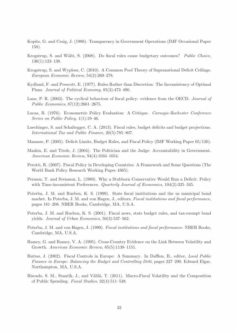
Kopits, G. and Craig, J. (1998). Transparency in Government Operations (IMF Occasional Paper158).

Krogstrup, S. and Walti, S. (2008). Do fiscal rules cause budgetary outcomes? Public Choice,136(1):123–138.

Krogstrup, S. and Wyplosz, C. (2010). A Common Pool Theory of Supranational Deficit Ceilings.European Economic Review, 54(2):269–278.

Kydland, F. and Prescott, E. (1977). Rules Rather than Discretion: The Inconsistency of OptimalPlans. Journal of Political Economy, 85(3):473–490.

Lane, P. R. (2003). The cyclical behaviour of fiscal policy: evidence from the OECD. Journal ofPublic Economics, 87(12):2661–2675.

Lucas, R. (1976). Econometric Policy Evaluation: A Critique. Carnegie-Rochester ConferenceSeries on Public Policy, 1(1):19–46.

Luechinger, S. and Schaltegger, C. A. (2013). Fiscal rules, budget deficits and budget projections.International Tax and Public Finance, 20(5):785–807.

Manasse, P. (2005). Deficit Limits, Budget Rules, and Fiscal Policy (IMF Working Paper 05/120).

Maskin, E. and Tirole, J. (2004). The Politician and the Judge: Accountability in Government.American Economic Review, 94(4):1034–1054.

Perotti, R. (2007). Fiscal Policy in Developing Countries: A Framework and Some Questions (TheWorld Bank Policy Research Working Paper 4365).

Persson, T. and Svensson, L. (1989). Why a Stubborn Conservative Would Run a Deficit: Policywith Time-inconsistent Preferences. Quarterly Journal of Economics, 104(2):325–345.

Poterba, J. M. and Rueben, K. S. (1999). State fiscal institutions and the us municipal bondmarket. In Poterba, J. M. and von Hagen, J., editors, Fiscal institutions and fiscal performance,pages 181–208. NBER Books, Cambridge, MA, U.S.A.

Poterba, J. M. and Rueben, K. S. (2001). Fiscal news, state budget rules, and tax-exempt bondyields. Journal of Urban Economics, 50(3):537–562.

Poterba, J. M. and von Hagen, J. (1999). Fiscal institutions and fiscal performance. NBER Books,Cambridge, MA, U.S.A.

Ramey, G. and Ramey, V. A. (1995). Cross-Country Evidence on the Link Between Volatility andGrowth. American Economic Review, 85(5):1138–1151.

Rattsø, J. (2002). Fiscal Controls in Europe: A Summary. In Dafflon, B., editor, Local PublicFinance in Europe: Balancing the Budget and Controlling Debt, pages 227–290. Edward Elgar,Northampton, MA, U.S.A.

Riscado, S. M., Stancık, J., and Valila, T. (2011). Macro-Fiscal Volatility and the Compositionof Public Spending. Fiscal Studies, 32(4):511–538.

32

Rodden, J. A. and Eskeland, G. S. (2003). Lessons and Conclusions. In Rodden, J. A., Eske-land, G. S., and Litvack, J., editors, Fiscal Decentralization and the Challenge of Hard BudgetConstraints, pages 35–83. MIT Press, Cambridge, MA, U.S.A.

Seegert, N. (2013). Optimal Taxation with Volatility: A Theoretical and Empirical Decomposition(Job Market Paper).

Serven, L. (2007). Fiscal Rules, Public Investment, and Growth (World Bank Policy ResearchWorking Paper 4382).

Tabellini, G. and Alesina, A. (1990). Voting on the Budget Deficit. American Economic Review,80(1):37–49.

Tomz, M. (2007). Reputation and International Cooperation: Sovereign Debt across Three Cen-turies. Princeton University Press, Princeton, NJ, U.S.A.

van der Ploeg, F. (2010). Political economy of prudent budgetary policy. International Tax andPublic Finance, 17(3):295–314.

Velasco, A. (2000). Debts and deficits with fragmented fiscal policymaking. Journal of PublicEconomics, 44(2):199–210.

von Hagen, J. (2010). Sticking to fiscal plans: the role of institutions. Public Choice, 144(3):487–503.

von Hagen, J. and Harden, I. H. (1995). Budget Processes and Commitment to Fiscal Discipline.European Economic Review, 39(3-4):771–779.

von Hagen, J. and Wolff, G. (2006). What do Deficits Tell us About Debt? Empirical Evidence onCreative Accounting with Fiscal Rules in the EU. Journal of Banking and Finance, 30(12):3259–3279.

Weingast, B. R., Shepsle, K. A., and Johnsen, C. (1981). The Political Economy of Benefitsand Costs: A Neoclassical Approach to Distributive Politics. Journal of Political Economy,89(4):642–664.

Weitzman, M. L. (1974). Prices vs. Quantities. Review of Economic Studies, 41(4):477–491.

Wyplosz, C. (2011). Fiscal Discipline: Rules Rather than Institutions. National Institute EconomicReview, 217(1):R19–R30.

Wyplosz, C. (2013). Fiscal rules: Theoretical issues and historical experiences. In Alesina, A.and Giavazzi, F., editors, Fiscal Policy after the Financial Crisis, pages 495–525. NBER Books,Cambridge, MA, U.S.A.

33