Certified Algorithms

for

Implicit Surfaces

Simon Plantinga

Contents

1 Introduction 1

1.1 Implicit surfaces . . . . . . . . . . . . . . . . . . . . . . . . . 11.1.1 Modeling . . . . . . . . . . . . . . . . . . . . . . . . . 21.1.2 Radial basis functions . . . . . . . . . . . . . . . . . . 4

1.2 Contour generators . . . . . . . . . . . . . . . . . . . . . . . . 41.3 Meshing . . . . . . . . . . . . . . . . . . . . . . . . . . . . . . 6

1.3.1 Continuation methods . . . . . . . . . . . . . . . . . . 61.3.2 Adaptive enumeration techniques . . . . . . . . . . . . 6

1.4 Surface reconstruction . . . . . . . . . . . . . . . . . . . . . . 81.5 Interval arithmetic . . . . . . . . . . . . . . . . . . . . . . . . 8

1.5.1 Interval analysis . . . . . . . . . . . . . . . . . . . . . 91.5.2 Interval Newton Method . . . . . . . . . . . . . . . . . 91.5.3 Affine arithmetic . . . . . . . . . . . . . . . . . . . . . 10

1.6 Implicit function theorem . . . . . . . . . . . . . . . . . . . . 101.7 Morse theory . . . . . . . . . . . . . . . . . . . . . . . . . . . 111.8 Overview and main results . . . . . . . . . . . . . . . . . . . . 12

1.8.1 Publications . . . . . . . . . . . . . . . . . . . . . . . . 13

2 Contour generators 15

2.1 Introduction . . . . . . . . . . . . . . . . . . . . . . . . . . . . 152.2 Contour generator and apparent contour . . . . . . . . . . . . 17

2.2.1 Contour generators of implicit surfaces . . . . . . . . . 172.2.2 Singular points of contour generators . . . . . . . . . . 192.2.3 Generic projections: fold and cusp points . . . . . . . 20

2.3 Evolving contours . . . . . . . . . . . . . . . . . . . . . . . . . 222.4 Transformations and normal forms . . . . . . . . . . . . . . . 25

2.4.1 Example: local model at a truncated cusp point . . . 262.5 Deriving local models . . . . . . . . . . . . . . . . . . . . . . 27

ii. Contents

2.5.1 Local model at a fold point . . . . . . . . . . . . . . . 28

2.5.2 Local model at a cusp point . . . . . . . . . . . . . . . 29

2.6 Time dependent contours . . . . . . . . . . . . . . . . . . . . 30

2.6.1 Lips and beak-to-beak bifurcations . . . . . . . . . . . 31

2.6.2 The swallowtail bifurcation . . . . . . . . . . . . . . . 34

3 Contour tracing 39

3.1 Introduction . . . . . . . . . . . . . . . . . . . . . . . . . . . . 39

3.2 Finding initial points . . . . . . . . . . . . . . . . . . . . . . . 40

3.3 Tracing step . . . . . . . . . . . . . . . . . . . . . . . . . . . . 40

3.3.1 Interval test . . . . . . . . . . . . . . . . . . . . . . . . 413.4 Evolving surfaces . . . . . . . . . . . . . . . . . . . . . . . . . 44

3.5 Results . . . . . . . . . . . . . . . . . . . . . . . . . . . . . . . 46

3.6 Conclusion and future research . . . . . . . . . . . . . . . . . 47

4 Isotopic Approximation 51

4.1 Introduction . . . . . . . . . . . . . . . . . . . . . . . . . . . . 51

4.2 Related work . . . . . . . . . . . . . . . . . . . . . . . . . . . 52

4.3 Curves . . . . . . . . . . . . . . . . . . . . . . . . . . . . . . . 54

4.4 Marching cubes revisited . . . . . . . . . . . . . . . . . . . . . 59

4.5 Octrees . . . . . . . . . . . . . . . . . . . . . . . . . . . . . . 64

4.6 Results . . . . . . . . . . . . . . . . . . . . . . . . . . . . . . . 69

4.7 Conclusion . . . . . . . . . . . . . . . . . . . . . . . . . . . . 69

5 Level sets of implicit functions 75

5.1 Introduction . . . . . . . . . . . . . . . . . . . . . . . . . . . . 75

5.2 Isotopic meshing with tetrahedra . . . . . . . . . . . . . . . . 76

5.3 Level sets . . . . . . . . . . . . . . . . . . . . . . . . . . . . . 79

5.3.1 Algorithm . . . . . . . . . . . . . . . . . . . . . . . . . 79

5.4 Results . . . . . . . . . . . . . . . . . . . . . . . . . . . . . . . 81

5.5 Conclusion and future work . . . . . . . . . . . . . . . . . . . 82

A Singularities of functions on surfaces 89

A.1 Non-degenerate singular points . . . . . . . . . . . . . . . . . 89

B The Morse Lemma with parameters 93

C Normal form of a Whitney fold 95

C.1 Fold points of good mappings . . . . . . . . . . . . . . . . . . 95

C.2 Normal form of a good map near a fold point . . . . . . . . . 98

C.3 Introducing parameters . . . . . . . . . . . . . . . . . . . . . 101

Contents iii.

Bibliography 103

iv. Contents

Chapter 1

Introduction

1.1 Implicit surfaces

Three-dimensional objects are extensively used in computer graphics appli-cations, such as computer aided design, animation, games and numerousother areas. These objects are often represented by triangle meshes. This isideal for objects with flat parts, such as buildings. Organic shapes however,have to be built up with a large number of tiny triangles to approximate thecurved surface, like geodesic domes approximating a sphere. For curved sur-faces, an implicit representation is a convenient alternative. In animation,ray-traced implicit surfaces are very useful, for example in modeling wateror deformable object [58, 26, 27]. Also, in computer aided geometric design,implicit curves and surfaces have several advantages over the more widelyused parametric representations [39].

Implicit surfaces are defined as the zero set of a function F : R3 → R.

See Figure 1.1. In this thesis we assume F is a smooth function defining aregular two-manifold, that is, the gradient does not disappear on the surface(see also Section 1.6).

For visualization of implicit surfaces raytracing can be used to createhigh-quality images. Several techniques have been suggested to improveraytracing computations for implicit functions [33, 34, 25]. However, for in-teractive visualization, raytracing is usually too slow. Approximating theimplicit surface with a conventional mesh allows fast rendering, taking fulladvantage of the hardware of graphics cards. This meshing of implicit sur-faces is one of the major topics of this thesis.

Accuracy is an important but often neglected issue in scientific visual-ization. Lopes [47] shows that inaccuracy in isosurfacing usually is due toincorrect topology. Several algorithms for implicit surfaces try to improveaccuracy by taking certain topological issues into consideration, for example

2. Chapter 1. Introduction

Figure 1.1: Implicit surface of the ‘chair’ function (Section 5.4).

by reconstructing the topology of a function ‘close to’ the implicit functionitself. An example is to use the trilinear interpolation of the function val-ues at a regular grid. Algorithms constructing meshes (regularly) isotopicto the implicit surface itself have only shown up recently. Regular isotopymeans that the mesh can be continuously deformed into the surface withoutleaving the embedded space, and is therefore an even stronger result thancorrect topology. However, we should note that for general implicit surfaces,it is difficult if not impossible to come up with a proof of correct topologywithout guaranteeing isotopy at the same time.

Regarding visualization, we should also mention the use of particle sys-tems. Small disks are distributed over the surface by using repelling forcesbetween these disks, together with an attracting force towards the surface.The resulting collection of disks gives a good indication of the shape of thesurface, without reconstructing its structure [71].

1.1.1 Modeling

One way to model implicit surfaces, originating from molecular modeling,is the use of blobs or metaballs (Figure 1.2). A single blob consists of aGaussian density function around a point, the corresponding isosurface beinga sphere. When using multiple blobs, the density functions interact witheachother, giving a smooth transition between the different balls. By varyingthe strenght and decay of the density functions, the size of the blobs and thedegree of interaction can be manipulated. Such a blobby surface is implicitlygiven by summing the individual density functions:

F(x, y, z) =∑

k

bke−akr

2k − T.

1.1. Implicit surfaces 3.

Here, rk represents the distance from (x, y, z) to the centre of blob k. Theparameters ak and bk determine the details of the individual blobs. Inparticular, negative values of bk can be used to produce dents instead ofbumps. The parameter T is a fixed threshold determining the particulariso-value.

In computer graphics, the Gaussian blobs are usually replaced by meta-balls or by soft objects, which are polynomial functions with compact sup-port. These metaballs provide a kind of digital clay to sculpt models bysmoothly adding or removing claylike pieces to the model.

For a metaball with radius d, the density function at distance r is givenby:

f(r) =

b(

1− 3r2

d2

)

, if 0 < r ≤ d3

32b(

1− rd

)2, if d

3< r ≤ d

0, if r > d

For soft objects, this density function is:

f(r) =

{1− 22r2

9d2 + 17r4

9d4 − 4r6

9d6 , if 0 < r ≤ d0, if r > d

As with the blob model, the implicit function consists of a weighted sumof these density functions.

Figure 1.2: Metaball objects.

Apart from this clay-like approach, constructive solid geometry (CSG)can also be applied to implicit surfaces. By performing simple arithmeticoperations on two functions, boolean operations on multiple implicit surfacescan be applied. For example, taking the maximum of two functions resultsin the union of two objects. However, these CSG objects are not smooth.

Implicit objects can also be blended together with a smooth transition,for example by using convolution surfaces [11].

4. Chapter 1. Introduction

1.1.2 Radial basis functions

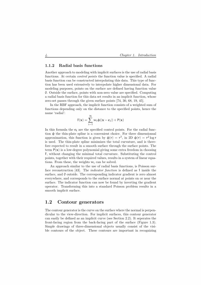
Another approach to modeling with implicit surfaces is the use of radial basisfunctions. At certain control points the function value is specified. A radialbasis function can be constructed interpolating this data. This type of func-tion has been used extensively to interpolate higher dimensional data. Formodeling purposes, points on the surface are defined having function value0. Outside the surface, points with non-zero value are specified. Computinga radial basis function for this data set results in an implicit function, whosezero-set passes through the given surface points [74, 30, 68, 19, 45].

In the RBF approach, the implicit function consists of a weighted sum offunctions depending only on the distance to the specified points, hence thename ‘radial’:

F(x) =

N∑

i=1

wiφ(|x − ci|) + P(x)

In this formula the ci are the specified control points. For the radial func-tion φ the thin-plate spline is a convenient choice. For three dimensionsalapproximation, this function is given by φ(r) = r3, in 2D φ(r) = r2 log ris used. The thin-plate spline minimizes the total curvature, and is there-fore expected to result in a smooth surface through the surface points. Theterm P(x) is a low-degree polynomial giving some extra freedom in choosingF, without changing the minimal total curvature. Substituting the controlpoints, together with their required values, results in a system of linear equa-tions. From these, the weights wi can be solved.

An approach similar to the use of radial basis functions, is Poisson sur-face reconstruction [43]. The indicator function is defined as 1 inside thesurface, and 0 outside. The corresponding indicator gradient is zero almosteverywhere, and corresponds to the surface normal at points on or near thesurface. The indicator function can now be found by inverting the gradientoperator. Transforming this into a standard Poisson problem results in asmooth implicit surface.

1.2 Contour generators

The contour generator is the curve on the surface where the normal is perpen-dicular to the view-direction. For implicit surfaces, this contour generatorcan easily be defined as an implicit curve (see Section 2.2). It seperates thefront-facing region from the back-facing part of the surface (Figure 1.3).Simple drawings of three-dimensional objects usually consist of the visi-ble contours of the object. These contours are important in recognizing

1.2. Contour generators 5.

the 3D shape, and are often used in so-called non-photorealistic render-ing [16, 50, 37], resulting in recognizable, drawing-like, artistic renderings ofthe object.

Figure 1.3: Torus with front-facing (dark) and back-facing (light) regionsseperated by the contour generator. The arrow indicates the view-direction.

Another application of contour generators is in view-dependent meshing.When fast rendering is important, such as in computer games, it is importantto use low-polygon models (i.e. having a low number of polygons). By usingsmooth lighting models, transitions between adjacent polygons appear tobe smoothened (Figure 1.4. The low number of polygons is hardly visible,except along the contours, where large, straight line segments form a jaggyoutline. The trick of view-dependent meshing, is to keep the polygon countlow over the largest part of the surface, and to refine the mesh along thecontour generator [3].

Figure 1.4: A smooth lighting model gives a low-polygon model of a spherea smooth looking surface, except for the jaggy contour.

6. Chapter 1. Introduction

1.3 Meshing

As stated earlier, a fast and convenient visualization method for implicitsurfaces is to generate a polyhedral mesh, usually a triangulation, approx-imating the surface. Several algorithms have been suggested for meshingimplicit surfaces [55]. These algorithms can be roughly divided into twogroups: continuation methods and adaptive enumeration techniques. Theformer group starts with a triangle close to the surface, and spreads outover the implicit surface by adding new triangles along the boundary ofthe already triangulated part. The latter group subdivides space into cellsand computes local approximations for the intersection of the surface with acell. By combining the local approximations a mesh is produced. The mostfamous example of this type of algorithm is Marching Cubes.

1.3.1 Continuation methods

Marching triangles [35] starts with a regular hexagon on the surface. Theboundary is called the front polygon. From points of the front polygon newtriangles of more or less uniform size are created to cover the surface. Bychecking the distance between points and front polygons, overlapping oftriangles is prevented.

Adaptive versions of marching triangles use triangle sizes depending onlocal curvature. The mesh spreads out over the surface until it is close toexisting triangles. This leaves untriangulated strips of the surface, that arefilled in a separate phase [1, 42].

Another adaptive version of continuation methods is Edge Spinning [20,51]. Here, triangles are constructed along the boundary of the already tri-angulated part, and ‘spinned’ around the connecting edge until the thirdvertex lies on the surface.

1.3.2 Adaptive enumeration techniques

Marching cubes Marching Cubes [49] subdivides space into a regulargrid of cubes. For implicit surfaces, the function sign at the vertices of acube are used to determine a local triangle mesh. Symmetry, rotation andflipping of function signs reduces the 256 possible cases to 15 different signconfigurations (Figure 1.5). Due to the ambiguities of some of these cases,Marching Cubes is not guaranteed to produce a two-manifold. An improvedversion that prevents this problem has been presented by Chernyaev [22].Another way to solve the problems of the original Marching Cubes has beensuggested by Lopes and Brodlie [46].

1.3. Meshing 7.

Figure 1.5: The 15 sign configurations of Marching Cubes.

These algorithms only require the function values at the vertices of aregular grid, and originate from meshing of voxel data, for example resultingfrom MRI scans. They can be easily adapted to implicit surfaces by onlyconsidering the function values at these vertices.

Yet another adaptation of Marching Cubes is Marching Tetrahedrons [67].Using a tetrahedral subdivision not only prevents the ambiguities of cubicalsubdivision, but also circumvented the recently expired patent on MarchingCubes. Tetrahedra can also be used for adaptive polygonization [40].

Bloomenthal [10] presents a continuation version of Marching Cubes, byonly meshing cubes along the boundary of the already meshed part of thesurface.

Similar algorithms exist for meshing with octrees instead of regular grids[61, 6, 7, 73, 38]. This enables local refinement of the mesh, for example inregions with higher curvature.

Dual contouring A dual version of Marching Cubes is called Dual Con-touring [41]. Here, triangular patches are not created for the cells of thesubdivision, but for the edges of the regular grid intersecting the surface.This algorithm uses Hermite data, that is, exact intersection points and nor-mals. For non-smooth level sets of voxel data, this enables Dual Contouring

8. Chapter 1. Introduction

to handle both sharp vertices and sharp edges.

1.4 Surface reconstruction

An important related topic in computer graphics is surface reconstruction.The problem is to construct a surface approximating a given point cloud, forexample the data from a 3D scanner. Several algorithms exist to generateboth meshes and implicit surfaces approximating these point clouds. Majorproblems in surface reconstruction are handling inaccurate data, sharp edgesand non-closed manifolds.

If the point sample is dense enough, topological guarantees can be givenfor the reconstructed surface. Sample density is usually defined in termsof the local feature size, which is defined as the distance of a point on thesurface to the medial axis. It is not difficult to imagine that in order todetermine the topology of the surface, point samples need to be denser inregions of high curvature, or where two parts of the surface are close toeachother.

For implicit surfaces, topologically correct approximations can be com-puted by creating a sufficiently dense point sample for this surface. Surfacereconstruction then gives a topologically correct mesh of the implicit sur-face [12]. The problem for generic implicit surfaces is to determine whatsufficiently dense means, since computing the local feature size is no trivialtask.

1.5 Interval arithmetic

The one-dimensional analogue of surface meshing is solving the equationF(x) = 0. To find all roots of a function F : R → R we can use intervalarithmetic. If the function is strictly positive over a given interval, thisinterval clearly contains no roots. If the function values at the endpoints ofan interval have opposite signs, and the function is strictly increasing, we canbe sure that the interval contains exactly one root. It is therefore sufficientto check whether the derivative over that interval is strictly positive. Byisolating the roots in disjoint intervals we have determined the ‘topology’ ofthe zero set. Also in higher dimensions interval arithmetic is an importanttool to guarantee correct topology.

1.5. Interval arithmetic 9.

1.5.1 Interval analysis

One way to prevent rounding errors due to finite precision numbers is to useinterval arithmetic [53]. Instead of numbers, intervals containing the exactsolution are computed. An inclusion function �f for a function f : R

m → Rn

computes for eachm-dimensional interval I (i.e. anm-box) an n-dimensionalinterval �f(I) such that

x ∈ I ⇒ f(x) ∈ �f(I)

An inclusion function is convergent if

width(I) → 0 ⇒ width(�f(I)) → 0

where the width of an interval is the largest width of I.For example if f : R → R is the square function f(x) = x · x, then a

convergent inclusion function is given by

�f([a, b]) =

{[min(a2, b2),max(a2, b2)], a · b < 0[0,max(a2, b2)], a · b ≥ 0

Inclusion functions exist for the basic operators and functions. To com-pute an inclusion function it is often sufficient to replace the standard num-ber type (e.g. double) by an interval type. Therefore, in practice almost allfunctions have convergent inclusion functions, which can be easily computedby using the same code together with an interval library.

We assume there are convergent inclusion functions for our implicit func-tion F and its derivatives, and will denote them by F (and similarly for thederivatives). From the context it will be clear when the inclusion functionis meant.

Interval arithmetic can be implemented using demand-driven precision.For the interval bounds, ordinary doubles can be used for fast computation.In the rare case that the interval becomes too small for the precision of adouble, a multi-precision number type can be used.

1.5.2 Interval Newton Method

For precision small intervals around the required value are used. Anotheruse of interval arithmetic is to compute function values over larger intervals.If for an implicit surface F = 0 and a box I we have 0 /∈ �F(I), we canbe certain that I contains no part of the surface. This observation can beextended to the Interval Newton Method, that finds all roots of a functionf : R

n → Rn in a box I.

10. Chapter 1. Introduction

The first part of the algorithm recursively subdivides the box, discardingparts of space containing no roots. If the boxes are ‘small enough’ a Newtonmethod refines the solutions and guarantees that all roots are found. Deter-mining when a box is small enough influences the speed of the algorithm,but has no effect on the guarantee to find all solutions. For the Newton stepwe solve

f(x) + J(I)(z − x) = 0,

where x is the centre of I, J is the Jacobian matrix of f and J(I) is the intervalmatrix of J over the interval I, resulting in an interval Y containing all rootsz of f. This interval can be used to refine I. Also, if Y ⊂ I there is a uniqueroot of f in I.

See [32] or [60] for the mathematical details. A more practical introduc-tion can be found in [62] or [65].

1.5.3 Affine arithmetic

Intervals can be regarded as a value together with an error bound. A draw-back of interval arithmetic is that it does not keep track of these error bounds.For example, if we compute X · X for X = [−1, 1], it results in the interval[−1, 1]. Stolfi proposed to use affine artithmetic, keeping track of which er-rors result from specific parameters [24, 66]. If we multiply X by itself, it‘knows’ that both terms have the same value. This results in X · X = [0, 1].Affine arithmetic therefore gives more accurate inclusion functions than in-terval arithmetic. However, due to the much more complicated computa-tions, affine arithmetic is considerably slower. In general, it is not clear ifthe use of affine arithmetic gives better results than using interval arithmeticwith for example an extra level of subdivision.

1.6 Implicit function theorem

An important tool in working with implicit functions is the implicit functiontheorem. It gives a sufficient condition to represent implicit surfaces locallyas the graph of a function. Though the general implicit function theoremis stated for functions F : R

m → Rn with m > n, we shall only use a few

simpler cases.For an implicit curve F : R

2 → R the implicit function theorem statesthat if F(x, y) = 0, where F is a continous function, and ∂F

∂y6= 0 at a point

p, then y can be written as a funtion of x in some neighbourhood of p.Stated otherwise, there exists a function g over that neighbourhood suchthat y = g(x).

1.7. Morse theory 11.

For a smooth function F : R2 → R this implies that the zero-set is a

regular curve, as long as the gradient does not disappear on F = 0. At apoint p with F(p) = 0, the curve is perpendicular to ∇F(p).

A similar result holds for implicit surfaces, that is, for F : R3 → R the

zero-set is a regular surface if ∇F(p) 6= 0 for F(p) = 0. Again, the gradient∇F(p) is perpendicular to the surface at point p.

For contour generators, we will also look at functions F : R3 → R

2. Inthis case, the zero set consists of a one-dimensional curve, if the determinantof the Jacobian matrix JF(p) does not disappear on the zero-set of F. Infact, this is easy to see by regarding the two components of F as two implicitsurfaces. The condition on the Jacobian tells us that the gradients of thesetwo surfaces are not parallel at p. The surfaces therefore have a properintersection, consisting of a one-dimensional curve.

1.7 Morse theory

Morse theory can be used to determine the topology of implicit surfaces fromthe critical points of a real function over the surface. This is best illustratedby considering implicit curves. By regarding the implicit function as a heightfunction, we can regard the zero set as the coastline of this landscape. Imag-ine that the water level rises. New coastlines appear when the water levelreaches the bottom of a valley, such that a new lake is created. Coastlinesof islands disappear when the water level reaches the highest point of theisland. Finally, coastlines can merge when two lakes or two islands grow to-gether. It is not difficult to see that this happens at points of the landscapewhere the ground is perfectly horizontal. This is exactly where the gradientof the height field function disappears. Moreover, examining the functionwe can determine the nature of the change in topology of the coastline. Theexamples given above correspond to local minima, local maxima and saddlepoints. The topology of the coastlines can now be determined by floodingthe entire landscape, slowly lowering the water level, and keeping track oftopological changes as the water level reaches so-called critical points, wherethe gradient disappears.

An important result is the following Morse lemma:

Lemma 1. Let p be a non-degenerate critical point of F (i.e., the Hessianmatrix of F at p is non-singular). Then there exists a neighbourhood U of pand smooth coordinates (x1, . . . , xn) on U such that xi(p) = 0 for all i, andF|U = F(p) − x21 − . . . − x2λ + x2λ+1 + . . . + x2n + higher order terms, where λis the index of F at point p.

12. Chapter 1. Introduction

Figure 1.6: An implicit curve as the coastline of a mathematical landscape.Islands merge as the water level drops.

A corollary of the Morse lemma is that non-degenerate critical points areisolated.

To apply Morse theory to implicit surfaces, information about the criti-cal points and their indices is required. In general this is not a trivial task,requiring interval arithmetic to construct unique enclosures of the criticalpoints. See [13] for a sketch of how to do this. For specific classes of func-tions, such as algebraic surfaces and certain metaball-like skeleton basedmodels [72], more convenient methods exist.

Another issue is finding a convenient Morse function on the surface, i.e.having no degenerate critical points with all critical levels being different.The particular choice of this function greatly influences the number of criticalpoints and therefore the complexity of determining the topology [54].

1.8 Overview and main results

Chapter 2 provides a mathematical framework for the robust computation ofcontour generators and apparent contours of implicit surfaces. Morse theoryis used to study the singularities of contour generators for evolving surfaces,or fixed surfaces with a moving viewpoint. We present a new derivation ofthe different types of singularities that can occur, together with local modelsthat can be used to classify these singularities. These results can be usedto update approximations of contour generators for dynamic surfaces withtopological guarantees.

In Chapter 3 we present a new algorithm for tracing implicit curves inhigher dimensional space, such that the resulting piecewise linear approx-imation is topological equivalent to the implicit curve itself. As far as we

1.8. Overview and main results 13.

know this is the first practical algorithm guaranteeing topological correct-ness. This algorithm is used to create a topologically correct approximationof a regular contour generator of a static surface. We also explain how a sim-ilar tracing process in a four-dimensional space can speed up the updatingof contour generators for evolving surfaces.

Chapter 4 presents one of the first algorithms to mesh implicit surfaces,such that the resulting mesh is isotopic to the implicit surface itself. Com-pared to conventional (not necessarily isotopic) meshing algorithms it addslittle overhead, and is therefore quite fast. In particular, to guarantee iso-topy, we do not have to do a relatively slow computation of critical points.Instead, a simple test based on interval arithmetic tests whether the localdeviation in gradient is small enough for a simple local approximation.

Finally, in Chapter 5 we examine how the same data structure used forisotopic approximation of implicit surfaces, can be used to move throughthe level sets of an implicit function. With a predetermined precision, thealgorithm produces meshes for the different level sets, and keeps track ofisotopy. If the level set moves close to singularities, isotopy cannot be guar-anteed. However, the algorithm indicates when and where this is the case,by isolating the problematic areas in small ‘red’ boxes. This way, areaswhere the isotopy class is not yet determined, are clearly indicated. In thiscase, further subdivision or analysis of the implicit function could be usedto examine the behaviour inside these red boxes.

1.8.1 Publications

Chapters 2 and 3 are to appear as Computing Contour Generators of Evolv-ing Implicit Surfaces in ACM Transactions on Graphics.

Chapter 4 and the tetrahedral meshing algorithm of Chapter 5 are toappear as Isotopic Meshing of Implicit Surface in The Visual Computer.

14. Chapter 1. Introduction

Chapter 2

Contour generators

2.1 Introduction

An important visibility feature of a smooth object seen under parallel projec-tion along a certain direction is its contour generator, also known as outline,or profile. The contour generator is the curve on the surface, separatingfront-facing regions from back-facing regions. This curve may have singu-larities if the direction of projection is non-generic. The apparent contouris the projection of the contour generator onto a plane perpendicular to theview direction. In many cases, drawing just the visible part of the apparentcontour gives a good impression of the shape of the object. In this chapter,we will not distinguish between visible and invisible parts of the contour gen-erator. Stated otherwise, we assume the surface is transparent. Generically,the apparent contour is a smooth curve, with some isolated singularities. SeeFigure 2.1.

The contour generator and the apparent contour play an important rolein computer graphics and computer vision. Rendering a polyhedral model ofa smooth surface yields a jaggy outline, unless the triangulation of the surfaceis finer in a neighbourhood of the contour generator. This observation has ledto techniques for view-dependent meshing and view-dependent refinementtechniques, cf. [3].

Also, to render a smooth surface it is sufficient to render only the partof the surface with front-facing normals, so the contour generator, beingthe boundary of the potentially visible part plays a crucial role here. Innon-photorealistic rendering [50] one just visualizes the apparent contour,perhaps enhanced by strokes indicating the main curvature directions of thesurface. This is also the underlying idea in silhouette rendering of implicitsurfaces [16]. In computer vision, techniques have been developed for partialreconstruction of a surface from a sequence of apparent contours correspond-

16. Chapter 2. Contour generators

-2 0 2

X

-2

0

2

Y

-2 -1 1 2

-3

-2

-1

1

2

3

Figure 2.1: A smooth surface (left), its apparent contour under parallelprojection along the z direction (middle), and its contour generator, seenfrom a different position (right). For generic surfaces (or, generic parallelprojections) the contour generator is a smooth, possibly disconnected curveon the surface, whereas the apparent contour may have isolated cusp points.

ing to a discrete set of nearby projection directions. We refer to the bookby Cipolla and Giblin [23] for an overview, and for a good introduction tothe mathematics underlying this chapter. Other applications use silhou-ette interpolation [31] from a precomputed set of silhouettes to obtain thesilhouette for an arbitrary projection. In computational geometry, rapidsilhouette computation of polyhedral models under perspective projectionwith moving viewpoints has been achieved by applying suitable preprocess-ing techniques [8].

This chapter presents a mathematical framework for the robust compu-tation of contour generators and apparent contours of implicit surfaces. Foran introduction to the use of implicit surfaces for smooth deformable objectmodeling we refer to Chapter 1, and to [57] and [9].

We first consider generic static views, where both the surface and thedirection of projection are static. Then we pass to time-dependent views,where the direction of projection changes with time. We derive conditionsthat locate the changes in the topology of the contour generator and the ap-parent contour. It turns out that generically there are three types of events,or bifurcations, leading to such a change in topology. These bifurcationshave been studied from a much more advanced mathematical point of view,where they are known under the names lips, beak-to-beak, and swallowtailbifurcation. See also [18]. For a nice non-mathematical description we re-fer to the book by Koenderink [44]. Also see [5] and [17] for a sketch ofsome of the mathematical details related to singularity theory. Some of theresults of this chapter are given in a complex analytic setting in [4]. Ourapproach is somewhere inbetween the level of Koenderink’s book and thesophisticated mathematical approach. We use only elementary tools, like

2.2. Contour generator and apparent contour 17.

the Inverse and Implicit Function Theorem, and finite order Taylor expan-sions. These techniques are used to design algorithms, in the same way asthe Implicit Function Theorem gives rise to Newton’s method.

The main result of this chapter is a general framework to examine and ap-proximate contour generators of implicit surfaces. We present a new deriva-tion of the different types of singularities, together with local models. Fore.g. algebraic surfaces, these local models can be used to classify singular-ities. As a first step to implementation, we present a new curve tracingalgorithm, with a correct topology of the output.

In Section 2.2 we present the framework, and discuss criteria for a pointon the contour generator and apparent contour to be regular. Section 2.3examines singularities under some time-dependent view, for example whenthe viewpoint moves or when the surface deforms. In section 2.4 we explainthe transformation to local models. Section 2.5 shows in detail how to derivelocal models near fold and cusp points. In section 2.6 we examine contoursfor time-dependent views. An overview of the existing theory used in thischapter is given in the appendices.

2.2 Contour generator and apparent contour

2.2.1 Contour generators of implicit surfaces

To understand the nature of regular and singular points of the contour gen-erator, and their projections on the apparent contour, we assume S is givenas the zero-set of a smooth function F : R

3 → R, so S = F−1(0). Smoothmeans that the required derivatives exist; for most of the results C3 willbe sufficient. In the section on evolving surfaces sometimes C5 is required.Furthermore, we assume that 0 is a regular value of F, i.e., the gradient ∇Fis non-zero at every point of the surface. The gradient vector ∇F(p) is thenormal of the surface at p, i.e., it is normal to the tangent plane of S atp. This tangent plane is denoted by Tp(S). If v is the direction of parallelprojection, then the contour generator Γ is the set of points at which thenormal to S is perpendicular to the direction of projection, i.e., p ∈ Γ iff thefollowing conditions hold:

F(p) = 0

〈∇F(p), v〉 = 0.(2.1)

For convenience, we assume that v = (0, 0, 1). Then the preceding equationsreduce to

F(x, y, z) = 0

Fz(x, y, z) = 0.(2.2)

18. Chapter 2. Contour generators

For arbitrary view directions the formulae become more complicated.It is more convenient to rotate the surface instead, by applying a rotationtransformation to the implicit function. Also, a linear skewing transfor-mation can be used. For view direction (α,β, 1) we consider the functionF(x−αz, y−βz, z) with view direction (0, 0, 1), and use the inverse skewingto move the approximation of the contour generator back to the originalsurface.

We assume that S is a generic surface, i.e. there are no degenerate sin-gular points on its contour generator. Some functions can yield degeneratecontour generators. For example, a cylinder has a two-dimensional contourgenerator for the view direction along its axis. Using a small perturbation,we can remove these degeneracies. In the case of the cylinder, the two-dimensional contour generator collapses to a one-dimensional curve. See forexample [65].

We now derive conditions for the contour generator Γ and the apparentcontour γ to be regular at a given point. Recall that a curve is regular ata certain point if it has a non-zero tangent vector at that point. The nextresult gives conditions in terms of the function defining the surface.

Proposition 2.

1. A point p ∈ Γ is a regular point of the contour generator if and only if

Fzz(p) 6= 0 or ∆(p) 6= 0, (2.3)

where ∆(p) is a Jacobian determinant defined by

∆(p) =∂(F, Fz)

∂(x, y)

∣

∣

∣

∣

p

=

∣

∣

∣

∣

Fx(p) Fy(p)

Fxz(p) Fyz(p)

∣

∣

∣

∣

.

2. A point p ∈ γ is a regular point of the apparent contour if and only if

Fzz(p) 6= 0. (2.4)

Proof. 1. The condition for p to be regular is

∇F(p) ∧ ∇Fz(p) 6= 0.

Since Fz(p) = 0, a straightforward calculation yields

∇F(p) ∧ ∇Fz(p) = Fzz · (Fy,−Fx, 0) +∂(F, Fz)

∂(x, y)· (0, 0, 1). (2.5)

Here all derivatives are evaluated at p. Since ∇F(p) = (Fx(p), Fy(p), 0) 6= 0,we see that (Fy,−Fx, 0) and (0, 0, 1) are linearly independent vectors. There-fore, the linear combination of these vectors in the right-hand side of (2.5)

2.2. Contour generator and apparent contour 19.

is zero iff the corresponding scalar coefficients are zero. The necessity andsufficiency of condition (2.3) is a straightforward consequence of this obser-vation.

2. Since ∇F(p) 6= 0 ∈ R3, and Fz(p) = 0, we see that (Fx(p), Fy(p)) 6= (0, 0).

Assuming Fy(p) 6= 0, we get

∂(F, Fz)

∂(y, z)

∣

∣

∣

∣

p

=

∣

∣

∣

∣

Fy FzFyz Fzz

∣

∣

∣

∣

p

= Fy(p)Fzz(p) 6= 0. (2.6)

Let p = (x0, y0, z0). Then, the Implicit Function Theorem yields locallydefined functions η, ζ : R → R , with η(x0) = y0 and ζ(x0) = z0, suchthat (2.2) holds iff y = η(x) and z = ζ(x). The contour generator is aregular curve parametrized as x 7→ (x, η(x), ζ(x)), locally near p, whereasthe apparent contour is a regular curve in the plane parametrized as x 7→(x, η(x)), locally near (x0, y0).

2.2.2 Singular points of contour generators

We apply the preceding result to detect non-degenerate singularities of con-tour generators of implicit surfaces. This result will be applied later in thischapter, when we consider contour generators of time-dependent surfaces.

Again, let the regular surface S be the zero set of a C3-function F : R3 →

R, for which 0 is a regular value. We consider the contour generator Γ of Sunder parallel projection along the vector v = (0, 0, 1). The equations for Γare

F = Fz = 0.

We consider the contour generator as the zero-set of the function Fz, re-stricted to S.

Corollary 3. Point p is a non-degenerate singular point of Γ iff the followingtwo conditions hold:

F(p) = Fz(p) = Fzz(p) =∂(F, Fz)

∂(x, y)

∣

∣

∣

∣

p

= 0, (2.7)

and Σ(p) 6= 0, where, for Fx(p) 6= 0,

Σ(p) = − Fx2 Fxzz

2 Fy2 + 2 Fx

3 Fxzz Fy Fyzz − Fx4 Fyzz

2

− 2 Fx3 Fxyz Fy Fzzz + 2 Fx

2 Fxy Fxz Fy Fzzz

+ Fx2 Fxxz Fy

2 Fzzz − Fx Fxx Fxz Fy2 Fzzz

− Fx3 Fxz Fyy Fzzz + Fx

4 Fyyz Fzzz,

(2.8)

20. Chapter 2. Contour generators

whereas, for Fy(p) 6= 0, we have

Σ(p) = − Fxzz2 Fy

4 + 2 Fx Fxzz Fy3 Fyzz − Fx

2 Fy2 Fyzz

2

− 2 Fx Fxyz Fy3 Fzzz + Fxxz Fy

4 Fzzz

+ Fx2 Fy

2 Fyyz Fzzz + 2 Fx Fxy Fy2 Fyz Fzzz

− Fxx Fy3 Fyz Fzzz − Fx

2 Fy Fyy Fyz Fzzz.

(2.9)

Proof. Condition (2.7) reflects the fact that p is a singular point of Fz|S,cf. (2.3), whereas (2.8) expresses non-degeneracy of this singular point. Con-dition (2.8) is obtained by a straightforward expansion of (A.3) (see ap-

pendix A), with G = Fz, and V = X as in (A.4), where λ =F0

xz

F0x

, F0z = F0zz = 0,

and F0yz =F0

y

F0xF0xz. Condition (2.9) is derived similarly.

2.2.3 Generic projections: fold and cusp points

In view of Proposition 2, regular points of the apparent contour are projec-tions of points (x, y, z) ∈ R

3 satisfying

F(x, y, z) = Fz(x, y, z) = 0, and Fzz(x, y, z) 6= 0.

This being a system of two equations in three unknowns, we expect thatthe regular points of the apparent contour form a one-dimensional subsetof the plane. Furthermore, the singular points of the apparent contour areprojections of points satisfying an additional equation, viz. Fzz(x, y, z) = 0,and are therefore expected to be isolated. This is true for generic surfaces.To make this more precise, we consider the set of functions F : R

3 → R,satisfying

( F(x, y, z), Fz(x, y, z), Fzz(x, y, z), ∆(x, y, z) ) 6= (0, 0, 0, 0), (2.10)

and

( F(x, y, z), Fz(x, y, z), Fzz(x, y, z), Fzzz(x, y, z) ) 6= (0, 0, 0, 0). (2.11)

If F satisfies (2.10), then Proposition 2 tells us that the contour generator Γof S = F−1(0) under parallel projection along v is a regular curve. Moreover,for a point (x, y, z) ∈ Γ there are two cases:

1. Fzz(x, y, z) 6= 0; in this case the point projects to a regular point (x, y)

of the apparent contour γ. Such a point is called a fold point of the

2.2. Contour generator and apparent contour 21.

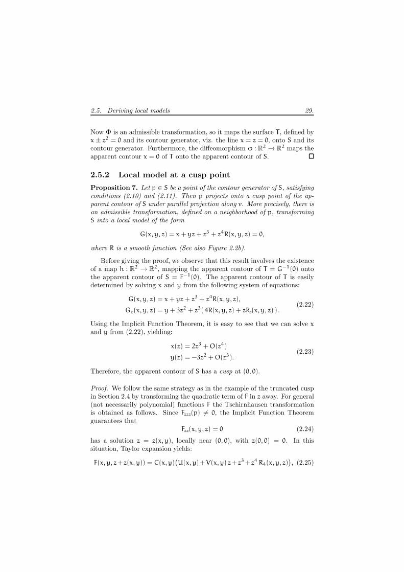
Figure 2.2: (a) A local model of the surface at a fold point is x + z2 = 0.Both the contour generator Γ , and the visible contour γ, are regular at thefold point, and its projection onto the image plane, respectively. (b) A localmodel at a cusp point is x+yz+z3 = 0. Here the contour generator is regular,but the apparent contour has a regular cusp.

contour generator. This terminology is justified by the local model ofthe surface near a fold point, viz.

x+ z2 = 0. (2.12)

See also Figure 2.2a. Here the contour generator is the y-axis in threespace, so the apparent contour is the y-axis in the image plane.

2. Fzz(x, y, z) = 0; in this case the point projects to a singular point (x, y)

of γ. Such a point is called a cusp point of the contour generator if, inaddition to (2.10), condition (2.11) is satisfied, i.e., if both ∆(x, y, z) 6=0 and Fzzz(x, y, z) 6= 0. In this case the surface has the following localmodel near the cusp point:

G(x, y, z) = x+ yz+ z3 = 0. (2.13)

See also Figure 2.2b. The local model G is sufficiently simple to allowfor an explicit computation of its contour generator and apparent con-tour: the former is parametrized by z 7→ (2z3,−3z2, z), the latter is aregular cusp parametrized by z 7→ (2z3,−3z2).

Intuitively speaking, a local model of the surface near a point is a ‘sim-ple’ expression of the defining equation in suitably chosen local coordinates.

22. Chapter 2. Contour generators

Usually, as in the cases of fold and cusp points, a local model is a low de-gree polynomial, which can be easily analyzed in the sense that the contourgenerator and the apparent contour are easily determined.

So far we have only considered parallel projection. The standard perspec-tive transformation [36], which moves the viewpoint to ∞, reduces perspec-tive projections to parallel projections. By deforming the surface using thistransformation, perspective projections can be computed by using parallelprojection on the transformed implicit function. Note that this perspectivetransform does not influence the smoothness of the implicit surface function.

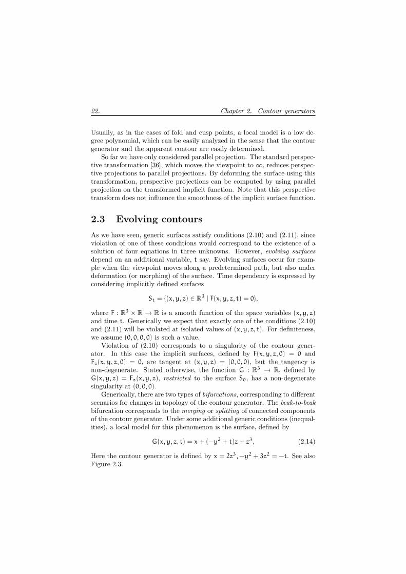
2.3 Evolving contours

As we have seen, generic surfaces satisfy conditions (2.10) and (2.11), sinceviolation of one of these conditions would correspond to the existence of asolution of four equations in three unknowns. However, evolving surfacesdepend on an additional variable, t say. Evolving surfaces occur for exam-ple when the viewpoint moves along a predetermined path, but also underdeformation (or morphing) of the surface. Time dependency is expressed byconsidering implicitly defined surfaces

St = {(x, y, z) ∈ R3 | F(x, y, z, t) = 0},

where F : R3 × R → R is a smooth function of the space variables (x, y, z)

and time t. Generically we expect that exactly one of the conditions (2.10)and (2.11) will be violated at isolated values of (x, y, z, t). For definiteness,we assume (0, 0, 0, 0) is such a value.

Violation of (2.10) corresponds to a singularity of the contour gener-ator. In this case the implicit surfaces, defined by F(x, y, z, 0) = 0 andFz(x, y, z, 0) = 0, are tangent at (x, y, z) = (0, 0, 0), but the tangency isnon-degenerate. Stated otherwise, the function G : R

3 → R, defined byG(x, y, z) = Fz(x, y, z), restricted to the surface S0, has a non-degeneratesingularity at (0, 0, 0).

Generically, there are two types of bifurcations, corresponding to differentscenarios for changes in topology of the contour generator. The beak-to-beakbifurcation corresponds to the merging or splitting of connected componentsof the contour generator. Under some additional generic conditions (inequal-ities), a local model for this phenomenon is the surface, defined by

G(x, y, z, t) = x + (−y2 + t)z + z3, (2.14)

Here the contour generator is defined by x = 2z3,−y2 + 3z2 = −t. See alsoFigure 2.3.

2.3. Evolving contours 23.

Figure 2.3: The beak-to-beak bifurcation. With respect to the local model(2.14) the bifurcation corresponds to t < 0 (left), t = 0 (middle), and t > 0(right).

Putting Gt(x, y, z) = G(x, y, z, t), we check that G0 satisfies (2.7) atp = (0, 0, 0), and that |Σ(p)| = −4. (In fact, G0x = 1, so all higher or-der derivatives of G0x vanish identically, so only the last term in the righthand side of (2.8) is not identically equal to zero.) Therefore, G0z |S has anon-degenerate singular point of saddle type at p. According to the Morselemma [28, 52], the level set of G0z |S through p consists of two regular curves,intersecting transversally at p, which concurs with Figure 2.3 (middle).

A second scenario due to the violation of (2.11) is the lips bifurcation,corresponding to the birth or death of connected components of the contourgenerator. Again, under some additional generic conditions a local modelfor this phenomenon is the surface, defined by

G(x, y, z, t) = x+ (y2 + t)z+ z3, (2.15)

Here the contour generator is defined by x = 2z3, y2 + 3z2 = −t. In par-ticular, for t > 0 the surface St has no connected component of the contourgenerator near (0, 0, 0), for t = 0, the point (0, 0, 0) is isolated on the contourgenerator, and for t < 0 there is a small connected component growing outof this isolated point as t decreases beyond 0. See also Figure 2.4.

As for the beak-to-beak bifurcation, we show thatG0|S has a non-degeneratesingular point at (0, 0, 0), which in this case is an extremum.

Violation of (2.11) involves the occurrence of a higher order singularityof the apparent contour. Note, however, that in this situation the contourgenerator is still regular at the point (x, y, z), cf. Proposition 2. Imposingsome additional generic conditions a local model for this type of bifurcation

24. Chapter 2. Contour generators

Figure 2.4: The lips bifurcation. Left: t < 0. Middle: t = 0. Right: t > 0.

is

G(x, y, z, t) = x+ yz + tz2 + z4 = 0. (2.16)

Here the apparent contour is parametrized as z 7→ (tz2 + z4,−2tz − 4z3).See also Figure 2.5.

Figure 2.5: The swallowtail bifurcation. Left: t < 0. Middle: t = 0. Right:t > 0.

2.4. Transformations and normal forms 25.

2.4 Transformations and normal forms

In Sections 2.2 and 2.3 we presented local models of various types of regularand singular points on contour generators and apparent contours, both forgeneric static surfaces, and for surfaces evolving generically in time. Theselocal models are low degree polynomials, which are easy to analyze, andwhich yet capture the qualitative behavior of the contour generator and theapparent contour in a neighbourhood of the point of interest. In this sectionwe explain more precisely what we mean by capturing local behavior.

Consider two regular implicit surfaces S = F−1(0) and T = G−1(0). Aninvertible smooth map Φ : R

3 → R3 for which

F ◦Φ = G (2.17)

maps T to S. In fact, we consider Φ to be defined only locally near somepoint of T , but we will not express this in our notation. The map Φ neednot map the contour generator of T onto that of S, however. To enforce this,we require that Φ maps vertical lines onto vertical lines, i.e., Φ should be ofthe form

Φ(x, y, z) = (h(x, y), H(x, y, z)), (2.18)

where h : R2 → R

2 and H : R3 → R are smooth maps. The map h is even

invertible, since Φ is invertible. To allow ourselves even more flexibility inthe derivation of local models, we relax condition (2.17) by requiring theexistence of a non-zero function ϕ : R

3 → R such that

F(Φ(x, y, z)) = ϕ(x, y, z)G(x, y, z). (2.19)

Definition 4. Let S = F−1(0) and T = G−1(0) be regular surfaces, near p =

(0, 0, 0) ∈ R3. An admissible local transformation from T to S, locally near

p, is a pair (Φ,ϕ), where ϕ : R3 → R is non-zero at p, and Φ : R

2×R → R3

is locally invertible near p, and of the form (2.18), such that (2.19) holds.We also say that Φ brings F in the normal form G.

If the surfaces S and T depend smoothly on k parameters, i.e., they aredefined by functions F : R

3×Rk → R and G : R

3×Rk → R, respectively, then

we require that the parameters are not mixed with the (x, y, z)-coordinates,i.e., we require that (2.19) is replaced with

F(Φ(x, y, z, µ)) = ϕ(x, y, z, µ)G(x, y, z, µ),

where Φ : R3 × R

k → R3 × R

k is of the form

Φ(x, y, z, µ) = (h(x, y, µ), H(x, y, z, µ), ψ(µ)).

26. Chapter 2. Contour generators

Then Φµ, defined by Φµ(x, y, z) = Φ(x, y, z, µ), maps Tµ to Sψ(µ), andpreserves contour generators. Furthermore, the map hµ : R

2 → R2, defined

by hµ(x, y) = h(x, y, µ), maps the apparent contour of Tµ onto that of Sψ(µ).

Proposition 5. If Φ is an admissible local transformation from T to S,locally near a point p on the contour generator of T , where Φ is of the form(2.18), then

1. Φ maps T to S, locally near p ∈ S;

2. Φ maps the contour generator of T to the contour generator of S, locallynear p;

3. h maps the apparent contour of T onto the apparent contour of S,locally near the projection π(p) ∈ R

2.

Proof. From (2.18) and (2.19) it is easy to derive

F(Φ(p)) = ψ(p)G(p),

Fz(Φ(p))Hz(p) = ψz(p)G(p) + ψ(p)Gz(p).

Since ψ(p) 6= 0, and Hz(p) 6= 0, we conclude that G(p) = Gz(p) = 0 iffF(Φ(p)) = Fz(Φ(p)) = 0.

2.4.1 Example: local model at a truncated cusp point

We now illustrate the use of admissible transformations by deriving a localmodel for the class of implicit surfaces defined as the zero set of a functionof the form:

F(x, y, z) = a(x, y) + b(x, y)z+ c(x, y)z2 + z3, (2.20)

with a(0, 0) = b(0, 0) = c(0, 0) = 0, and

∂(a, b)

∂(x, y)

∣

∣

∣

∣

0

6= 0. (2.21)

Note that the local model x+ y z+ z3 = 0, derived in Section 2.2 for a cusppoint, belongs to this class. Our goal is to show that the latter is indeed alocal model for all surfaces of the type (2.20). Since F(0) = Fz(0) = Fzz(0) = 0,and

∂(F, Fz)

∂(x, y)

∣

∣

∣

∣

0

=∂(a, b)

∂(x, y)

∣

∣

∣

∣

0

6= 0,

we see that 0 ∈ R3 is a regular point of the contour generator of S, whereas

(0, 0) is a singular point of the apparent contour, cf. Proposition 2

2.5. Deriving local models 27.

As a first step towards a normal form of the implicit surface, we apply theTschirnhausen transformation z 7→ z − 1

3c(x, y) to transform the quadratic

term (in z) in F away. More precisely,

F(x, y, z − 13c(x, y)) = a(x, y) − 1

3b(x, y) c(x, y) + 2

27c(x, y)3

+ (b(x, y) − 13c2(x, y)) z + z3

= G(ϕ(x, y), z),

where G(x, y, z) = x+ yz + z3, and

ϕ(x, y) = (a(x, y) − 13b(x, y) c(x, y) + 2

27c(x, y)3,

b(x, y) − 13c(x, y)2 ).

It is not hard to check that the Jacobian determinant of ϕ at 0 ∈ R2 is equal

to∂(a, b)

∂(x, y)

∣

∣

∣

∣

0

,

so ϕ is a local diffeomorphism near 0 ∈ R2. Let ϕ be its inverse, then,

puttingΦ(x, y, z) = (ϕ(x, y), z − 1

3c(ϕ(x, y)),

we getF ◦Φ(x, y, z) = G(x, y, z).

In other words, the admissible transformation Φ brings F into the normalform G. In particular, it maps the surface T = G−1(0) and its contourgenerator onto S = F−1(0), and ϕ maps the apparent contour of T onto theapparent contour of S.

2.5 Deriving local models

In this section, we derive local models of an implicit surface near fold andcusp points of contour generators. The local model for the fold point is asstated in Section 2.2, the one for the cusp point is slightly weaker in the sensethat it includes terms of higher order. To derive these models, we use onlyelementary means, like the Implicit Function Theorem and Taylor expansionup to finite order. Although these tools are strong enough to derive theessential qualitative features of the contour generator and apparent contourat a fold or a cusp point, they are not strong enough to obtain the simplepolynomial form for the cusp as stated earlier. Although the cubic modelfor the cusp (See Figure 2.2b) can be obtained by elementary means, the

28. Chapter 2. Contour generators

derivation is quite involved, cf. [70]. Even worse, the polynomial models ofthe contour generator of evolving surfaces (See Figures 2.3, 2.4, and 2.5)can only be obtained using sophisticated methods from Singularity Theory.Therefore, our more modest goal will be to obtain a local model only for thelower order part of the implicit function, which is sufficient for our purposes.See Proposition 7 for a more precise statement.

2.5.1 Local model at a fold point

Proposition 6. Let p ∈ S be a regular point of the contour generator of S,and let its image under parallel projection along v be a regular point of theapparent contour of S. Then there is an admissible transformation, bringingS into the normal form x± z2 = 0 (See also Figure 2.2a).

Proof. Let p = 0 ∈ R3 be a regular point of the contour generator of S =

F−1(0), and let its projection (0, 0) be a regular point of the apparent contour.Then F(0) = Fz(0) = 0, and Fzz(0) 6= 0. Consider F as a 2-parameter familyof real-valued univariate functions depending on the parameters (x, y), i.e.,

F(x,y)(z) = F(x, y, z).

Then F(0,0) has a non-degenerate singularity at 0 ∈ R, and hence the functionF(x,y) has a non-degenerate singularity z = ζ(x, y), depending smoothly onthe parameters (x, y), such that ζ(0, 0) = 0. According to the Morse Lemmawith parameters, cf. Appendix B, there is a local diffeomorphism (x, y, z) 7→(x, y, Z(x, y, z)) on a neighborhood of 0 ∈ R

3, such that

F(x, y, Z(x, y, z)) = α(x, y) ± z2.

where α(x, y) = F(x, y, ζ(x, y)). Since (α0x, α0y) = (F0x , F

0y ) 6= (0, 0), let us

assume that α0x 6= 0. Then there is a local diffeomorphism ϕ : R2 → R

2 ofthe form ϕ(x, y) = (ξ(x, y), y), such that

α(ϕ(x, y)) = x.

In fact, ξ(x, y) is the solution of the equation α(ξ, y)−x = 0, with ξ(0, 0) = 0.The existence and local uniqueness follows from the Implicit Function Theo-rem. Furthermore, ξ0xα

0x = 1, which proves that ϕ is a local diffeomorphism.

Therefore,F ◦Φ(x, y, z)) = x± z2,

where the local diffeomorphism Φ : R3 → R

3 is defined by

Φ(x, y, z) = (ξ(x, y), y, Z(ξ(x, y), y, z)).

2.5. Deriving local models 29.

Now Φ is an admissible transformation, so it maps the surface T , defined byx± z2 = 0 and its contour generator, viz. the line x = z = 0, onto S and itscontour generator. Furthermore, the diffeomorphism ϕ : R

2 → R2 maps the

apparent contour x = 0 of T onto the apparent contour of S.

2.5.2 Local model at a cusp point

Proposition 7. Let p ∈ S be a point of the contour generator of S, satisfyingconditions (2.10) and (2.11). Then p projects onto a cusp point of the ap-parent contour of S under parallel projection along v. More precisely, there isan admissible transformation, defined on a neighborhood of p, transformingS into a local model of the form

G(x, y, z) = x + yz + z3 + z4R(x, y, z) = 0,

where R is a smooth function (See also Figure 2.2b).

Before giving the proof, we observe that this result involves the existenceof a map h : R

2 → R2, mapping the apparent contour of T = G−1(0) onto

the apparent contour of S = F−1(0). The apparent contour of T is easilydetermined by solving x and y from the following system of equations:

G(x, y, z) = x+ yz+ z3 + z4R(x, y, z),

Gz(x, y, z) = y+ 3z2 + z3( 4R(x, y, z) + zRz(x, y, z) ).(2.22)

Using the Implicit Function Theorem, it is easy to see that we can solve xand y from (2.22), yielding:

x(z) = 2z3 +O(z4)

y(z) = −3z2 +O(z3).(2.23)

Therefore, the apparent contour of S has a cusp at (0, 0).

Proof. We follow the same strategy as in the example of the truncated cuspin Section 2.4 by transforming the quadratic term of F in z away. For general(not necessarily polynomial) functions F the Tschirnhausen transformationis obtained as follows. Since Fzzz(p) 6= 0, the Implicit Function Theoremguarantees that

Fzz(x, y, z) = 0 (2.24)

has a solution z = z(x, y), locally near (0, 0), with z(0, 0) = 0. In thissituation, Taylor expansion yields:

F(x, y, z+z(x, y)) = C(x, y)(

U(x, y)+V(x, y) z+z3+z4 R4(x, y, z))

, (2.25)

30. Chapter 2. Contour generators

where R4 is a smooth function, and

C(x, y) = 16Fzzz(x, y, z(x, y)).

U(x, y) = F(x, y, z(x, y))/C(x, y)

V(x, y) = Fz(x, y, z(x, y))/C(x, y)

(2.26)

Note that C(0, 0) 6= 0. Furthermore, U(0, 0) = V(0, 0) = 0. Note that thereis no quadratic term in (2.25), because Fzz(x, y, z(x, y)) = 0.

The right hand side of (2.25) is in fact the form of F after the parameter-dependent change of coordinates (x, y, z) 7→ (x, y, z + z(x, y)). We try topolish (2.25) further by applying additional admissible transformations ofthe parameters (x, y) and the variable z. To this end, observe that

∂(U,V)

∂(x, y)

∣

∣

∣

∣

(0,0)

=6

F0zzz

∂(F, Fz)

∂(x, y)

∣

∣

∣

∣

(0,0)

6= 0.

Therefore, there is an invertible smooth local change of x, y-coordinates ϕ :

R2 → R

2 such that

U ◦ϕ(x, y) = x, and V ◦ϕ(x, y) = y. (2.27)

Therefore

F(ϕ(x, y), z + z(ϕ(x, y) ) ) = C(x, y)G(x, y, z),

whereG(x, y, z) = x+ y z + z3 + z4 R(x, y, z),

with R(x, y, z) = R4(ϕ(x, y), z). In other words: G is a local model of F.

2.6 Time dependent contours

If we allow the direction of projection to change over time, or, equivalently,fix the direction of projection and allow the surface to depend on time, theimplicit function, defining the surface, depends on four variables (x, y, z, t),where t corresponds to time. In this situation, we expect one of the condi-tions (2.10) and (2.11) to be violated at isolated values of (x, y, z, t). See alsothe description of evolving contours in Section 2.2. In this section, we deriveapproximate local models for these degenerate situations, cf. Figures 2.4, 2.3and 2.5.

As said before, we consider a smooth function F : R3 × R → R, which

defines a time-dependent surface St = (Ft)−1(0), where Ft : R3 → R is

defined by Ft(x, y, z) = F(x, y, z, t).

2.6. Time dependent contours 31.

-5 0 5

X

-5

0

Y

-5 0 5

X

-10

-5

0

Y

-5 0 5

X

-10

-5

0

Y

-5 0 5

X

-10

-5

0

Y

-6 -4 -2 2 4

-8

-6

-4

-2

2

4

-6 -4 -2 2 4

-10

-8

-6

-4

-2

2

-6 -4 -2 2 4

-10

-8

-6

-4

-2

2

-6 -4 -2 2 4

-12

-10

-8

-6

-4

-2

2

Figure 2.6: A beak-to-beak bifurcation. Top row: a sequence of views of asmooth surface. Middle row: the corresponding apparent contours. Bottomrow: blow-up of the apparent contour near the bifurcation event.

2.6.1 Lips and beak-to-beak bifurcations

The occurrence of lips and beak-to-beak bifurcations are associated with aviolation of condition (2.10).

Proposition 8. Let p be a non-degenerate singular point of the contourgenerator for t = t0, i.e.,

F(p, t0) = Fz(p, t0) = Fzz(p, t0) =∂(F, Fz)

∂(x, y)

∣

∣

∣

∣

(p,t0)

= 0, and Fzzz(p, t0) 6= 0,

(2.28)and

Σ(p) 6= 0,

where Σ(p) is as in (2.8) or (2.9). Moreover, assume that the matrix

(

F0x F0y F0t

F0xz F0yz F0tz

)

has rank two. (2.29)

32. Chapter 2. Contour generators

Then the surface has a local model at (p, t0) of the form

G(x, y, z, t) = x+(

σy2 + α(x, t))

z+ z3 + z4R(x, y, z, t),

where σ = sign(Σ(p)), with Σ(p) defined by (2.8) or (2.9), R is a smoothfunction for (x, y, z, t) near (0, 0, 0, 0), and ∂α

∂t(0, 0) 6= 0.

Remark 9. Before giving the proof, we observe that the contour generatoris determined by the equations G = Gz = 0, i.e.,

x+ (σy2 + α(x, y)) z+ z3 = O(z4),

(σy2 + α(x, y)) z + 3z2 = O(z3).

Solving this system for x and y yields

x = 2 z3 +O(z4)

σy2 + 3 z2 = −α(x, t) +O(z3).

Since α(0, 0) = 0, it is easy to see that the singularity of the contour generatorfor t = 0 is of saddle type if σ = −1, and corresponds to an extremum ifσ = +1. The former case corresponds to a beak-to-beak bifurcation, thelatter to a lips bifurcation. We have a scenario as depicted in Figure 2.3 and2.4, respectively, where it depends on the sign of ∂α

∂t(0, 0) whether we have

to read the Figure from left-to-right or from right-to-left, as t passes zerofrom negative to positive values.

Proof. For ease of notation we assume that p = (0, 0, 0) and t0 = 0. Ourapproach is as in the derivation of the local normal form near a cusp point,i.e., we again consider the equation

Fzz(x, y, z, t) = 0. (2.30)

cf. (2.24). Since Fzzz(0, 0, 0, 0) 6= 0, there is a locally unique solution z =

ζ(x, y, t) of (2.30), with ζ(0, 0, 0) = 0. Also in this situation, Taylor expan-sion yields:

F(x, y, z+z(x, y), t) = C(x, y, t)(

U(x, y, t)+V(x, y, t) z+z3+z4 R4(x, y, z, t))

,

where R4 is a smooth function, and

C(x, y, t) = 16Fzzz(x, y, z(x, y, t)).

U(x, y, t) = F(x, y, z(x, y, t), t)/C(x, y, t)

V(x, y, t) = Fz(x, y, z(x, y, t), t)/C(x, y, t)

2.6. Time dependent contours 33.

Also in this case C(0, 0, 0) 6= 0, and U(0, 0, 0) = V(0, 0, 0) = 0. To avoidsuperscripts, we introduce the functions u, v : R

2 → R, defined by u(x, y) =

U(x, y, 0), and v(x, y) = V(x, y, 0). In this case we have

∂(U,V)

∂(x, y)

∣

∣

∣

∣

(0,0)

=6

F0zzz

∂(F, Fz)

∂(x, y)

∣

∣

∣

∣

(0,0)

= 0, (2.31)

so, unlike the situation at a cusp point, we don’t have the normal form(x, y) for the pair (u, v). Yet, we can obtain a normal form as stated in theProposition. To this end introduce the map Ψ : R

2 × R → R2, defined by

Ψ(x, y, t) = (U(x, y, t), V(x, y, t)). (2.32)

It follows from (2.32) that the Jacobian determinant J = UxVy−UyVx of Ψsatisfies

J(0, 0, 0) = 0. (2.33)

Since, moreover,

(u0x, u0y) =

6

F0zzz(F0x, F

0y) 6= (0, 0), (2.34)

the derivative of the mapψ : R2 → R

2, defined by ψ(x, y) = (u(x, y), v(x, y))

at (0, 0) ∈ R2 has rank one.

This observation brings us to the context of Singularity Theory, in par-ticular the theory of normal forms of generic maps from the plane to theplane. Whitney’s paper [70] presents a local normal form for the two typesof generic singularities of this type of maps, viz. the fold and the cusp. Assaid before, although, or perhaps, because, this paper uses elementary tools,the technical details are quite involved. We refer the reader to Appendix Cfor a rather self-contained derivation of the Whitney fold, fine-tuned to ourcurrent context.

To make the link with Whitney’s result more precise, observe that theJacobian determinant j of ψ satisfies the identity j(x, y) = J(x, y, 0). Since∇u(0, 0) 6= (0, 0), cf. (2.34), Proposition 19, or rather its parametrized ver-sion presented in Section C.3, guarantees the existence of a change of pa-rameters ϕ(x, y, t) of the form ϕ(x, y, t) = (·, ·, t), such that

U ◦ϕ(x, y, t) = x, and V ◦ϕ(x, y, t) = σy2 + α(x, t).

Here α is a smooth function with α(0, 0) = 0, and

σ = sign(〈∇u(0, 0),∇j(0, 0)⊥〉) = sign(−u0xj0y + u0yj

0x).

A straigthforward, but tedious computation shows that

−u0xj0y + u0yj

0x = Σ(p),

34. Chapter 2. Contour generators

where Σ(p) is defined by (2.8) or (2.9). Therefore,

F(ϕ(x, y, t), z + z(ϕ(x, y, t) ) ) = C(x, y, t)G(x, y, z, t),

whereG(x, y, z) = x+ (σy2 + α(x, t)) z+ z3 + z4 R(x, y, z),

with R(x, y, z) = R4(ϕ(x, y, t), z). In other words: G is a local model ofF.

-2 0 2

X

-4

-2

0

2

4

Y

-2 0 2

X

-4

-2

0

2

4

Y

-2 0 2

X

-2

0

2

Y

-3 -2 -1 1 2 3

-4

-2

2

4

-3 -2 -1 1 2 3

-4

-2

2

4

-3 -2 -1 1 2 3

-3

-2

-1

1

2

3

Figure 2.7: A swallowtail bifurcation. Top row: a sequence of views of asmooth surface. Middle row: the corresponding apparent contours. Bottomrow: blow up of the apparent contour near the bifurcation event.

2.6.2 The swallowtail bifurcation

In this section we study the discontinuous change of the apparent contourassociated with a violation of (2.11), whereas (2.10) still holds. In this casethe contour generator is regular.

2.6. Time dependent contours 35.

Proposition 10. Let F : R3 × R → R be such that at (p, t0) ∈ R

3 × R thefollowing conditions are satisfied:

F(p, t0) = Fz(p, t0) = Fzz(p, t0) = Fzzz(p, t0) = 0. (2.35)

If at (p, t0) the generic conditions:

Fzzzz(p, t0) 6= 0,∂(F, Fz)

∂(x, y)

∣

∣

∣

∣

(p,t0)

6= 0, and∂(F, Fz, Fzz)

∂(x, y, t)

∣

∣

∣

∣

(p,t0)

6= 0. (2.36)

are satisfied, then F has a local model at (p, t0) of the form

G(x, y, z, t) = x + y z+w(x, y, t) z2 + z4 + z5 R(x, y, z, t), (2.37)

with w(0, 0, t) = α t+O(t2), where

α =4!

∆0 F0zzzz

∂(F, Fz, Fzz)

∂(x, y, t)

∣

∣

∣

∣

(0,0,0)

6= 0. (2.38)

In particular, there is a time-dependent change of coordinates ht : R2 → R

2,mapping the apparent contour of St onto the apparent contour of (Gt)−1(0),which has a parametrization of the form z 7→ ( x(z, t), y(z, t) ), where:

x(z, t) = w0(t) z2 − 2w0(t)w0x(t) z3 − (3+w0(t)W(t)) z4 + X(z, t) z5

y(z, t) = −2w0(t)z + 4w0(t)w0y(t) z2 − (2+w0(t)W(t)) z3 + Y(z, t) z4,

with

w0(t) = w(0, 0, t) = α t+O(t2)

w0x(0) = −4!

∆0 F0zzzz

∂(Fz, Fzz)

∂(x, y)

∣

∣

∣

∣

0

,

w0y(0) =4!

∆0 F0zzzz

∂(F, Fzz)

∂(x, y)

∣

∣

∣

∣

0

,

W(0) = w0x + 4 (w0y )2.

Remark 11. The parametrization of the apparent contour is of the form

x(z, t) =(

α t+O(t2))

z2 +O(t) z2 −(

3+O(t))

z4 +O(z5),

y(z, t) =(

−2α t+O(t2))

z +O(t) z2 −(

2+O(t2))

z3 +O(z4).

For α > 0, the evolution of the apparent contour is as the one depicted inFigure 2.5, whereas for α < 0 the evolution corresponds to reading the latterfigure from right to left.

36. Chapter 2. Contour generators

Proof. As before, we assume that p = (0, 0, 0) and t0 = 0. As in the Tschirn-hausen transformation, we try to transform the cubic term away by consid-ering the equation

Fzzz(x, y, z, t) = 0. (2.39)

Since Fzzzz(0, 0, 0, 0) 6= 0, there is a locally unique solution z = ζ(x, y, t) of(2.39), with ζ(0, 0, 0) = 0. Also in this situation, Taylor expansion yields:

F(x, y, z + ζ(x, y, t), t) = C(U+ Vz+Wz2 + z4 + z5R(x, y, z, t)),

where R is a smooth function, and

C = C(x, y, t) = 14!Fzzzz(x, y, ζ(x, y, t), t),

U = U(x, y, t) = F(x, y, ζ(x, y, t), t)/C(x, y, t),

V = V(x, y, t) = Fz(x, y, ζ(x, y, t), t)/C(x, y, t),

W = W(x, y, t) = 12Fzz(x, y, ζ(x, y, t), t)/C(x, y, t).

In particular, U(0, 0, 0) = 0, V(0, 0, 0) = 0, W(0, 0, 0) = 0, and C(0, 0, 0) 6= 0.Since, according to (2.35):

∂(U,V)

∂(x, y)

∣

∣

∣

∣

(0,0,0)

=4!

F0zzzz

∂(F, Fz)

∂(x, y)

∣

∣

∣

∣

(0,0,0,0)

=4!∆0

F0zzzz6= 0,

we see that the map ψ : R2 × R → R

2 × R, defined by

ψ(x, y, t) = (U(x, y, t), V(x, y, t), t),

is a local diffeomorphism, which has an inverse of the form

ϕ(x, y, t) = (ξ(x, y, t), η(x, y, t), t),

i.e.,

U ◦ϕ(x, y, t) = x and V ◦ϕ(x, y, t) = y. (2.40)

Putting

Φ(x, y, z, t) = (ξ(x, y, t), η(x, y, t), z, t),

we see that Φ is an admissible transformation bringing F into the normalform G = F ◦Φ, which is of the form

G(x, y, z, t) = x+ y z+w(x, y, t)z2 + z4 +O(|z|5),

2.6. Time dependent contours 37.

where

w(x, y, t) = W(ξ(x, y, t), η(x, y, t), t) = Fzz(ξ(x, y, t), η(x, y, t), t).

Therefore w(0, 0, 0) = 0. Furthermore,

wt(0, 0, 0) =4!

F0zzzz(F0xzz ξ

0t + F0yzz η

0t + F0tzz)

From (2.40) we derive

U0x ξ0t +U0y η

0t +U0t = 0,

V0x ξ0t + V0y η

0t + V0t = 0.

In other words:(

F0x F0y

F0xz F0yz

) (

ξ0t

η0t

)

=

(

−F0t

−F0zt

)

Using Cramer’s rule, we obtain

ξ0t = −1

∆0

∣

∣

∣

∣

∣

F0t F0y

F0zt F0yz

∣

∣

∣

∣

∣

, and η0t = −1

∆0

∣

∣

∣

∣

∣

F0x F0t

F0xz F0zt

∣

∣

∣

∣

∣

.

Therefore,

w0t = −4!

∆0 F0zzzz

(

F0xzz

∣

∣

∣

∣

∣

F0t F0y

F0zt F0yz

∣

∣

∣

∣

∣

+ F0yzz

∣

∣

∣

∣

∣

F0x F0t

F0xz F0zt

∣

∣

∣

∣

∣

− F0tzz

∣

∣

∣

∣

∣

F0x F0y

F0xz F0yz

∣

∣

∣

∣

∣

)

=4!

∆0 F0zzzz

∣

∣

∣

∣

∣

∣

∣

∣

F0x F0y F0t

F0xz F0yz F0zt

F0xzz F0yzz F0zzt

∣

∣

∣

∣

∣

∣

∣

∣

=4!

∆0 F0zzzz

∂(F, Fz, Fzz)

∂(x, y, z)

∣

∣

∣

∣

0

. (2.41)

By a similar computation we obtain:

w0x = −4!

∆0 F0zzzz

∂(Fz, Fzz)

∂(x, y, z)

∣

∣

∣

∣

0

. (2.42)

and

w0y =4!

∆0 F0zzzz

∂(F, Fzz)

∂(x, y, z)

∣

∣

∣

∣

0

. (2.43)

38. Chapter 2. Contour generators

Finally, we can solve x and y as functions of (z, t) from the set of equationsG(x, y, z, t) = Gz(x, y, z, t) = 0, with G as in (2.37). A straightforwardcomputation yields:

x(0, t) = 0

y(0, t) = 0

xz(0, t) = 0

yz(0, t) = −2w(0, 0, t)

xzz(0, t) = 2w(0, 0, t)

yzz(0, t) = 8w(0, 0, t)wy(0, 0, t)

xzzz(0, t) = −12w(0, 0, t)wy(0, 0, t)

yzzz(0, t) = −12(

2+ 4w(0, 0, t)wy(0, 0, t)2 + 2w(0, 0, t)2wyy(0, 0, t)+

w(0, 0, t)wx(0, 0, t))

xzzzz(0, t) = 24(

3+ 4w(0, 0, t)wy(0, 0, t)2 + 2w(0, 0, t)2wyy(0, 0, t)+

w(0, 0, t)wx(0, 0, t))

The low order Taylor expansions of x(z, t) and y(z, t), as stated in Proposi-tion 10 are obtained by combining these expressions with the identities forw0t , w

0x, and w0y in (2.41), (2.42), and (2.43), respectively.

Chapter 3

Contour tracing

3.1 Introduction

In this chapter we will introduce a new curve tracing algorithm with topo-logical guarantees. Our goal is to approximate the contour generator by apiecewise linear curve. This initial approximation can then be maintainedunder some time-dependent view. To this end the singularities of the contourgenerator for an evolving view or surface can be precomputed using intervalanalysis. Since the topology doesn’t change between these singularities, theinitial contour generator can be updated continuously, until we reach a timewhere a singularity arises. The local model at this singularity indicates howthe topology has to be updated. See Section 2.4 in the previous chapter.

Note that for a singularity of the contour generator of a time-dependentsurface, we have

F(x, y, z, t)

Fz(x, y, z, t)

Fzz(x, y, z, t)

∆(x, y, z, t)

= 0,

with ∆ as in Proposition 2.

These singularities can therefore be considered as the zeroes of a functionfrom R

4 to R4. Using the Interval Newton Method, we can find all t for which

a singularity occurs.

For the initial contour generator, generically there are no singularities.The construction consists of two steps.

Firstly, for each component of the contour generator we have to find aninitial point to start the tracing process. Interval analysis will enable usto find points on all components of the contour generator. These (regular)points serve as starting points for the tracing process.

40. Chapter 3. Contour tracing

Secondly, we trace the component by stepping along the contour gener-ator. For each starting point we trace the component, by moving from apoint pi to the next point pi+1. We take a small step in the direction of thetangent to the contour generator at pi. Then, we move the resulting pointback to the contour generator, giving us pi+1. An interval test guaranteesthat we stay on the same component, without skipping a part. If the testfails, we decrease the step size and try again, until the interval test succeeds.If we reach the initial point p0, the component is fully traced.

3.2 Finding initial points

To be able to trace all components of the contour generator, we have to findat least one point on each component from where we can start the tracingprocess.

A point p on the contoru generator satisfies both F(p) = 0 and Fz(p) = 0.A tangent vector to the contour generator at p can be found by computing

w(p) = ∇F(p) ∧ ∇Fz(p) =

FyFzz−FxFzz

FxFyz − FyFxz

.

Since the components of the contour generator are bounded, closed curves,there are at least two points on each component where the x-component ofw(p) disappears, i.e. where FyFzz = 0.

Let R, S : R3 → R

3 be the functions

R(p) =

F(p)

Fz(p)

Fy(p)

and S(p) =

F(p)

Fz(p)

Fzz(p)

The Interval Newton Method finds all roots of R and S. These roots result ina list of (regular) initial points. During the tracing process we can identifywhich initial points lie on the same component.

3.3 Tracing step

Starting at an initial point we now trace the component by taking smallsteps along the contour generator in the direction of the tangent vector. Tocontrol the step size we will use the normalized tangent vectors. The stepsize is crucial in guaranteeing correct topology of the approximation.

3.3. Tracing step 41.

Let T(x) be the normalized vector field

T(x) =∇F(x) ∧ ∇Fz(x)

‖∇F(x) ∧ ∇Fz(x)‖.

For x on the contour generator, T(x) is a tangent vector at x. From pi wefirst move to q0 = pi + δT(pi), where δ determines the step size. To moveback to the contour generator, we alternately move towards F = 0 and Fz = 0

by replacing qi by

qi+1 = qi −F(qi)∇F(qi)‖∇F(qi)‖2 towards F

qi+2 = qi+1 −Fz(q

i+1)∇Fz(qi+1)‖∇Fz(qi+1)‖2

towards Fz

until ‖qi+2 − qi‖ is sufficiently small. The resulting point is the next pointon the contour generator, pi+1. For this new point we perform the intervaltest (explained below) to determine whether pipi+1 is a good approximationof the contour generator. If not, we decrease δ (e.g. by setting it to δ/2),and repeat the tracing step from pi. To prevent δ from decreasing to 0 wemultiply it by 1.2 after each successful step.

3.3.1 Interval test

The main problem of existing tracing methods is that for a fixed step size,there is always a possibility of accidentally jumping to another componentof the contour generator, or of skipping a part (Figure 3.1). This preventstopologically correct approximation of curves. Using interval arithmetic wecan ensure that the step size is small enough to guarantee correct topology.

F = 0

Fz = 0

T(pi)

pi

pi+1

Figure 3.1: Left: T (pi) is a tangent to the intersection of F = 0 and Fz = 0.Right: a fixed step size can miss part of the contour generator.

To assure that pipi+1 is a good approximation for the contour generator,first we construct a sphere S with centre pi, that contains pi+1. Then we

42. Chapter 3. Contour tracing

take the bounding box B of S:

B = [pix −D,pix +D] × [piy −D,piy +D] × [piz −D,piz +D],

where D = ‖pi+1 − pi‖. Over this box we compute the interval

I = 〈T(pi), T(B)〉,

where T(B) contains all normalized vectors∇F(s) ∧ ∇Fz(t)

‖∇F(s) ∧ ∇Fz(t)‖, with s, t ∈ B.

Lemma 12. If I > 12

√2, (i.e. ∀i ∈ I : i > 1

2

√2), then the part of the contour

generator within S consists of a connected part of a single component of thecontour generator (Figure 3.2).

T(pi)

pi

pi+1S

B

Figure 3.2: The sphere containing the line segment, and its bounding box.

Proof. We define G(x) = 〈x − pi, T(pi)〉. The level sets of G are planesperpendicular to T(pi). Let f : R

3 → R3 be the function

f(x) =

F(x)

Fz(x)

G(x)

.

Suppose there are two points x and y of the contour generator in B, lyingin a plane perpendicular to T(pi), i.e. f(x) = f(y) = (0, 0, θ) for some θ.According to the Mean Value Theorem, there are points s and t on xy where

∇F(s)∇Fz(t)T(pi)

(y− x) =

0

0

0

For x 6= y, we find that 〈∇F(s) ∧ ∇Fz(t), T(pi)〉 = 0 (all vectors in a planeperpendicular to y − x). Since s, t ∈ B this contradicts the interval test.

3.3. Tracing step 43.

Therefore, within box B each plane perpendicular to T(pi) contains at mostone point of the contour generator.

The interval condition I > 12

√2 implies that the angle between T(pi) and

T(x) is at most π4

for all x ∈ B and therefore also for x ∈ Γ ∩B. The contourgenerator lies in a cone C around T(x) (fig. 3.3) with top angle π

2, for if it

leaves the cone at point a, then 〈T(pi), T(a)〉 would be smaller than 12

√2.

It can only leave the sphere in S ∩ C. In this part of the sphere the contourgenerator cannot re-enter S, because that would require an entry point bwhere 〈T(pi), T(b)〉 < 1

2

√2. Therefore, there can only be a single connected

component of the contour generator within sphere S.

T(pi)pi

S

C

Figure 3.3: The contour generator lies within a cone.

If the interval test succeeds, we can use the same sphere S to removeredundant points from the initial point list. If there are points in the listthat lie within S, they must be part of the component we are tracing, sothey can be discarded.

To test whether the component is fully traced, we test if the currentsphere S overlaps the sphere of the initial point p0. If it does, testing

〈pi+1 − pi, p0 − pi〉 > 0

tells us whether we are done with this component (otherwise we just startedthe trace and are still moving away from p0).

The interval bound is valid if the centre of the cube is on the contourgenerator. Since pi is in general close to, but not on the contour generator,in practice we take a slightly larger bound (e.g. by multiplying the radiusby 1.1). Also, D should be slightly larger than ‖pi+1 − pi‖, to preventpi+1 from being too close to other parts of the contour generator outside S.Again, multiplying by 1.1 should suffice to prevent rounding errors.

For algorithms on implicit surfaces it is difficult to derive a complexitybound, because timing results depend not only on the complexity of the

44. Chapter 3. Contour tracing

surface, but also on the behaviour of the function outside the surface, andon the accuracy of the convergent inclusion functions. For algebraic surfacesit might be possible to derive the complexity, similar to [2].

3.4 Evolving surfaces

Time-dependent surfaces occur for example if the viewpoint moves along afixed path, or if the surface changes shape under a continuous deformation(morphing). We assume that the transformation is also a smooth function,e.g. rotation. For a time-dependent surface F(x, y, z, t) = 0 there is no needto compute the initial points on the contour generator for each t. Instead,we can trace the initial points as time evolves. Recall that the initial pointsare zeroes of the functions R, S : R

4 → R3:

R(x, y, z, t) =

F(x, y, z, t)

Fz(x, y, z, t)

Fy(x, y, z, t)

and S(x, y, z, t) =

F(x, y, z, t)

Fz(x, y, z, t)

Fzz(x, y, z, t)

For time-dependent surfaces, these are 1-dimensional curves in R4. These

curves can be traced similarly to the contour generator itself, i.e. by steppingalong the curve using a step size such that the interval inequality (I > 1

2

√2)

is satisfied.

The tangent vector to the curve is perpendicular to the gradients of thethree components of R and of S. As time evolves, generically initial pointsare created and destroyed in pairs. This happens when the tangent vectoris perpendicular to the t-axis. Otherwise, according to the implicit functiontheorem there exists a unique solution.

For R the tangent vector can be found using

Ker

Fx Fy Fz FtFxz Fyz Fzz FztFxy Fyy Fyz Fyt

A solution (t1, t2, t3, t4) in the kernel with∑ti = 1 can be found by

adding a row [1, 1, 1, 1] to the matrix, resulting in a 4×4-matrixM, provideddet(M) 6= 0. Since R(x, y, z, t) = 0 we have Fz = Fy = 0. Using Cramer’srule to solve

Fx Fy Fz FtFxz Fyz Fzz FztFxy Fyy Fyz Fyt1 1 1 1

t1t2t3t4

=

0

0

0

1

,

3.4. Evolving surfaces 45.

we find a tangent vector for the curve:

∣

∣

∣

∣

∣

∣

0 0 FtFyz Fzz FztFyy Fyz Fyt

∣

∣

∣

∣

∣

∣

,−

∣

∣

∣

∣

∣

∣

Fx 0 FtFxz Fzz FztFxy Fyz Fyt

∣

∣

∣

∣

∣

∣

,

∣

∣

∣

∣

∣

∣

Fx 0 FtFxz Fyz FztFxy Fyy Fyt

∣

∣

∣

∣

∣

∣

,−

∣

∣

∣

∣

∣

∣

Fx 0 0

Fxz Fyz FzzFxy Fyy Fyz

∣

∣

∣

∣

∣

∣

This tangent vector is perpendicular to the t-axis if

F

FzFyFx

= 0 or

F

FzFy

F2yz − FyyFzz

= 0

The first equality has no solutions, since the surface does not contain singu-larities.

Similarly, for S we have:

Ker

Fx Fy Fz FtFxz Fyz Fzz FtzFxzz Fyzz Fzzz Ftzz

For the tangent vector of S we find:

0

@

˛

˛

˛

˛

˛

˛

Fy 0 FtFyz 0 FtzFt Ftz Ftzz

˛

˛

˛

˛

˛

˛

,−

˛

˛

˛

˛

˛

˛

Fx 0 FtFxz 0 FtzFxzz Fzzz Ftzz

˛

˛

˛

˛

˛

˛

,

˛

˛

˛

˛

˛

˛

Fx Fy FtFxz Fyz FtzFxzz Fyzz Fzzz

˛

˛

˛

˛

˛

˛

,−

˛

˛

˛

˛

˛

˛

Fx Fy 0

Fxz Fyz 0

Fxzz Fyzz Fzzz

˛

˛

˛

˛

˛

˛

1

A

This vector is perpendicular to the t-axis if

F

FzFzzFzzz

= 0 or

F

FzFzz

FxFyz − FyFxz

= 0

The first equality corresponds to swallowtail bifurcations, the second equalitycorresponds to a singularity of the contour generator.

For dynamic surfaces depending on a single parameter, computing thefour-dimensional initial points shows us at which time steps the set of initialpoints for the contour generator changes. As long as the time parameter tdoes not pass such a time value, we can adjust the position of the currentinitial points to the new value of t, by tracing a small part of the four-dimensional curve. For small time steps this requires only a small numberof 4D tracing steps. The time to compute the new contour generator istherefore only slightly larger than the time required for the tracing phase,

46. Chapter 3. Contour tracing

removing the time required to find the initial points. When t does pass oneof the precomputed values, generically a pair of initial points of the contourgenerator is created or destroyed. In this case we can adjust the set of initialpoints by adding or removing a pair of points.

Doing more preprocessing, we could also precompute the approximationof the entire 4D curve, enabling us to find the initial points for any fixed t,by intersecting this 4D curve with the t-plane.

For a single parameter function, we can handle evolving surfaces such aslevel sets of an implicit function, or moving along a one-dimensional viewpath. Arbitrary view directions require two parameters. In this case we alsohave other types of bifurcations, such as the butterfly bifurcation. How tohandle contour generators of surfaces with more than one parameter remainsan open problem.

3.5 Results

We have implemented the computation of the static contour generator, usingthe interval classes and interval Newton solver from the c-xsc [56] library.

The table below shows the results on a Pentium 2.80GHz, running Linux.The implicit surface was transformed with a shearing to change the viewdirection from the default (0, 0, 1). The resulting contour generators areshown in Figure 3.4, 3.5, and 3.6 for the tangle cube, and in Figure 3.7 and 3.8for the non-algebraic surface. The table shows the number of contours, thetotal number of line segments, and timing results for the two phases: findingthe initial points, and tracing the contour generator.Surface Contours Segments Initial pts Tracing Total

Tangle (0.095, 0.295, 1) 4 4148 3.6s 2.2s 5.8sTangle (0.09, 0.29, 1) 8 3940 3.4s 1.5s 4.9sTangle (0.08, 0.25, 1) 8 3184 3.0s 1.0s 4.0sNon-alg. (0.2, 0.4, 1) 62 11869 22.1s 3.4s 25.5sNon-alg. (0.8, 0.4, 1) 29 23812 75.3s 6.8s 82.1s

At the moment the (inclusion) functions and derivatives are hard-codedinto the implementation, since we do not have an interval newton implemen-tation working together with automatic differentiation. A solution would beto use a code generator that outputs inclusion functions of all derivatives.The lack of such a preprocessor makes experimenting with 4D curves te-dious. However, as mentioned in the previous section, the time required forupdating the contour generator for small time steps is only slightly largerthan the results in the table under ‘Tracing’.

The preprocessing requires computing the initial points of the 4D curve.We have computed these points for the tangle cube, for the view direction

3.6. Conclusion and future research 47.

moving along the one-dimensional path (x− tz, y− (0.2+ t)z, z). This pathincludes the views shown in Figure 3.4 and Figure 3.5. We separately solvedthe three sets of equations from the previous section: F = Fz = Fy = F2yz −

FyyFzz = 0, F = Fz = Fzz = Fzzz = 0 and F = Fz = Fzz = FxFyz − FyFxz = 0.The following table shows the results for these three equations, as well asthe total time for computing the initial points of the 4D curve. We solvedover the intervals [0, 1] and over the ten subintervals of width 0.1. The finalrow gives the sum over these ten smaller intervals.

t Interval F2yz − FyyFzz Fzzz FxFyz − FyFxz Total

[0, 1] 977s 7894s 1972s 10843s[0.0, 0.1] 0.2s 9.0s 13.5s 22.7s[0.1, 0.2] 0.7s 23.9s 21.2s 45.8s[0.2, 0.3] 1.7s 52.4s 27.2s 81.3s[0.3, 0.4] 4.6s 90.8s 30.8s 126.2s[0.4, 0.5] 7.7s 132.5s 34.1s 174.3s[0.5, 0.6] 11.4s 181.7s 40.4s 233.5s[0.6, 0.7] 17.4s 227.6s 51.6s 296.6s[0.7, 0.8] 33.8s 298.2s 67.3s 399.3s[0.8, 0.9] 78.4s 388.6s 93.1s 560.1s[0.9, 1.0] 70.7s 476.2s 127.9s 674.8s10 intervals 226.6s 1880.9s 507.1s 2614.6

The time for solving over the interval [0, 1] is just over three hours,whereas solving over ten intervals of width 0.1 takes less than 44 minutes.This indicates that the interval Newton implementation in the c-xsc libraryis far from optimal. Results can be greatly improved by subdividing thesearch space first. For algebraic functions such as the tangle cube, of courseother methods for solving systems of equations are available.

3.6 Conclusion and future research

In Chapters 2 and 3 we presented a framework for the analysis of an implicitsurface near regular and singular points of its contour generator and apparentcontour, and also derived conditions for detecting changes of topology ofthese visibility features in generic one-parameter families of implicit surfaces.

We developed an algorithm to compute a topologically correct approxi-mation of curves, in particular of the initial contour generator. A dynamicstep size, combined with an interval test, guarantees that no part of thecontour generator is skipped.

For further experiments we require an interval Newton method work-ing together with automatic differentiation, or a preprocessor generatinginclusion functions for the partial derivatives of the implicit function. More

48. Chapter 3. Contour tracing

Figure 3.4: Surface with contour generator, contour generator alone, and

detail of the contour generator of the tangle cube x4 − 5x2 + y4 − 5y2 + z4 −

5z2 + 10 = 0. The view direction (0.095, 0.295, 1). The contour generator isplotted as the set of spheres, such that larger spheres indicate a larger stepsize. The actual contour generator connects the centres of these spheres. Thedetail shows the contour generator on the top left of the tangle cube, shownfrom above.

Figure 3.5: Contour generator of the tangle cube, with view direction(0.09, 0.29, 1).

research needs to be done on solving systems of equations. The intervalNewton method used is far from optimal. Faster solvers are required for apractical implementation of dynamic contours. In particular, for algebraicsurfaces other methods should be considered. For this class of surfaces, itis also easier to examine the singularties, using the theory on local models.This information can be used to construct singular contours.

3.6. Conclusion and future research 49.

Figure 3.6: Contour generator of the tangle cube, with view direction(0.08, 0.25, 1).

Figure 3.7: Contour generator of the non-algebraic surface −0.4(sin(5x) +

sin(5y) + cos(5z)) + 0.1x2 + 0.3y2 + 0.2z2 − 0.5, view direction (0.2, 0.4, 1).

Figure 3.8: Contour generator of the non-algebraic surface, view direction(0.8, 0.4, 1).

50. Chapter 3. Contour tracing

Chapter 4

Isotopic Approximation

4.1 Introduction

Implicit functions provide a convenient representation of smooth surfaces.However, piecewise linear approximations are often required, for examplefor visualization. Meshing algorithms can only compute function values at afinite number of points. Since grid based schemes can miss important detailsof the surface, correct topology usually cannot be guaranteed. To capturethe global properties of implicit surfaces, we somehow need to extract infor-mation about the surroundings of these points. Lipschitz conditions give abound on the gradient and can therefore sometimes discard the neighbour-hood of a point. Another tool that can be used is interval arithmetic.

In this chapter we present an algorithm that creates a regularly isotopicapproximation of implicit curves in R

2 and of implicit surfaces in R3. Reg-

ularly isotopic means that the approximation is equivalent to the curve orsurface under continuous deformation within the embedding space. In par-ticular, the approximation has the same topology as the implicit manifold.Correct topology is important to determine connectedness, and for examplein constructing an initial mesh for time-dependent surfaces (e.g. morphing).Our implicit surface meshing algorithm subdivides space using an octree.Interval arithmetic is used to decide which cells of the octree require furthersubdivision. For each leaf of the resulting octree a local approximation isconstructed.

The algorithm given in this chapter falls in the category of enumera-tion methods. A novelty is that we use a fast and simple interval test todecide which cells need subdivision, in such a way that we can guaranteeisotopy. Compared to other enumeration methods it adds little overhead,and is therefore quite fast. In particular, we do not need to compute thecritical points of the implicit function.

52. Chapter 4. Isotopic Approximation

The octree based subdivision is very flexible. For example we coulddefine a minimal subdivision level to improve the Hausdorff distance betweenthe surface and the approximation. A maximal subdivision level could beused to improve the speed of the meshing process and to handle surfaceswith singularities. In this case colour coding of the mesh could be used toidentify the (arbitrarily small) regions where the approximation might betopologically incorrect.

In section 4.2 we give an overview of the existing techniques for implicitcurve and surface approximation. Section 4.3 explains our approximation al-gorithm for implicit curves. After giving the algorithm, we will prove that theresulting piecewise linear approximation is isotopic to the curve itself. Sinceboth the algorithm and its proof will be generalized to the three-dimensionalcase, this section also provides an introduction to the meshing of implicitsurfaces. In section 4.4 we provide a first step towards our meshing algo-rithm, by adapting the well-known marching cubes algorithm to constructisotopic approximations. Section 4.5 extends the previous section by usingoctrees instead of a regular grid, thereby greatly reducing the complexityof both the algorithm and the resulting mesh. Results of the algorithmsare shown in section 4.6. Finally, in section 4.7 we discuss some possibleimprovements and possible changes to our approximation scheme.

Main contribution This chapter presents a new algorithm to approx-imate not necessarily algebraic regular implicit curves and surfaces. Forsurfaces, it is one of the first schemes guaranteeing that the resulting meshis isotopic to the implicit surface. For curves, it is the first practical algo-rithm giving this guarantee. Since we do not need to compute the criticalpoints of the implicit function, both algorithms are fast enough to be ofpractical use. Also, they can easily be adapted to improve the accuracyof the approximation and to deal with singular surfaces. We expect thatthe algorithm generalizes to isotopic approximation of all codimension onemanifolds in Euclidean spaces.

4.2 Related work

Several algorithms exist for the approximation of implicit curves and sur-faces, but very few can guarantee topological correctness. Since we can onlycompute function values at a finite number of points, there is a risk of missingimportant details of the curve or surface. Some approximation algorithmsdepend on a user specified value to give a trade-off between accuracy andspeed. For these methods it is not clear what level of accuracy is required tocapture the topology of the implicit manifold. Algorithms that do guarantee

4.2. Related work 53.

a topologically correct result depend either on extra information about theunderlying implicit function (e.g. algebraicity of surfaces or bounds on theLipschitz conditions), or on interval arithmetic.

In this section we will give an overview of the different existing techniquesfor approximation of implicit curves and surfaces.

Curves The schemes for approximation of implicit curves can be roughlydivided into continuation methods and adaptive enumeration techniques.

Continuation methods approximate the curve or surface by first findingseed points on all components, and then using these as starting points fortracing the components.

In [16] an implicit curve (in this case a contour in R3) is approximated

using a predictor-corrector method. Initial points are found by shooting ran-dom rays to the surface and by moving from the first intersection point alongthe surface towards the contour. In [59] we adapted this method to guar-antee topological correctness of an approximation of the contour generator,but to achieve this the relatively slow interval Newton method was required.Also, a small step size for the tracing process is required to guarantee thatthe resulting approximation is isotopic to the traced component.

Approximation schemes based on adaptive enumeration start with abounding box and subdivide until the cells are ‘small enough’, for exam-ple by looking at the local curvature. Then, for each cell of the subdividedbox a local approximation is constructed. In [48] interval arithmetic is usedto get a good approximation of implicit curves. The size of the subdividedcells depends on the geometry of the curve, such that in areas with highcurvature the level of detail is also higher. However, to terminate the sub-division process, the method requires user-specified bounds on cell size, andon the variation of the normalized gradient within a cell. Although the edgelength varies with the curvature of the curve, it cannot guarantee correcttopology.

As in this chapter, [63] uses parametrizability to subdivide a quadtree.This algorithm guarantees topological correctness, but because of a slightlyweaker test for parametrizability, it requires a large number of (slow) intervalNewton searches for intersection points.

Surfaces A continuation algorithm is given in [35]. Starting with a seedpoint on the surface, a triangulation is generated by expanding over thesurface, along the boundary of the already triangulated part. As with curves,this algorithm depends on seed points, and on a user-specified step size. Thetriangles of the resulting mesh have more or less the same size, independent

54. Chapter 4. Isotopic Approximation

of the geometry of the surface. An improvement of this algorithm using adynamic triangle size is given in [1].

Enumeration methods use either a regular grid or an octree to subdi-vide space. Regular grids are used in the well-know marching cubes al-gorithm [49]. The main purpose of these methods is to mesh sampledvoxel data, but they can easily be adapted to approximate implicit sur-faces. In [10], cubes are constructed along the surface. Although this savesexamining a large number of grid cells, there is a risk of missing componentsof the implicit surface. Another improvement of marching cubes is givenin [22]. The linear variation along an edge used in marching cubes, is ex-tended to trilinear variation over the cube, using the function values at theeight corners of the cube. The algorithm guarantees that the approxima-tion has the same topology as the isosurface of this trilinear function. Forimplicit surfaces there is no such guarantee.

For dynamic surfaces, critical points and their indices indicate when,where and how the topology changes. This can be used to update the topol-ogy of the triangulation, as in [64]. Also, the shrinkwrap algorithm [69] canbe adapted to use critical points for updating the topology [15].

An algorithm for isotopic meshing based on critical points is given in [13].It is based on Morse theory to determine the topology, and therefore requiresa priori knowledge of the critical points of the implicit surface, as well as oftheir indices.

Finally, sampling based algorithms construct a sufficiently dense sampleof points on the surface, such that surface reconstruction on this point setresults in a homeomorphic approximation. To construct such a sampling,in [14] bounds on the distance to the medial axis are needed, while in [21] thecritical points of heightfunctions on the surface and on intersection curvesare required. Also, both algorithms assume that the intersection points of agiven line segment with the surface can be computed. These Delaunay basedalgorithms result in a better mesh quality, but for generic implicit surfacesit is very difficult to meet these assumptions.

4.3 Curves

In this section we will introduce an algorithm to construct a piecewise linearapproximation of an implicit curve S, such that the approximation and Shave the same (regular) isotopy. The construction is based on a quadtree.After subdivision this quadtree is balanced, i.e. the tree is further subdivideduntil two neighbouring squares differ at most a factor two in size. Balancingdoes not increase the complexity of the tree.

4.3. Curves 55.

Possible improvements regarding accuracy and singularities will be dis-cussed in Section 4.7 and in the next chapter.

Let S = F−1(0) be a bounded implicit curve, where F : R2 → R is a smooth

function and 0 is a regular value of F, i.e. the gradient ∇F is non-zero at everypoint of the curve. The following algorithm constructs an isotopic piecewiselinear approximation of S. Details are explained right after the presentationof the algorithm.

Algorithm ApproximateCurve(F, B)Input. An implicit function F, and a square bounding box B.Output. A piecewise linear approximation of the curve F = 0.1. Initialize a quadtree T to the bounding square B of F = 0.2. Subdivide T until for all leavesC we have 0 /∈ 2F(C)∨〈2∇F(C),2∇F(C)〉 >

0.

3. BalanceQuadtree(T )4. for each edge of the quadtree5. do if the signs of F at its two endpoints are opposite6. then construct a vertex at the midpoint of the edge7. for each leaf C of quadtree T8. do if the leaf contains two vertices9. then connect the vertices by a line segment10. if the leaf contains four vertices11. then find the two vertices on the same side and connect each

of them to the other adjacent vertex

Note that a single side of a cell may consist of two quadtree edges, if theneighbouring cell along that side is subdivided. See Figures 4.18 and 4.19.Each cell of the quadtree is therefore surrounded by four to eight quadtreeedges.

The construction of the approximating edges handles only a few differentcases of vertex placement on the boundary of a cell: either two vertices, orfour vertices with two of them along one side of the cell. In the correct-ness proof we will show that these are the only possible cases satisfying oursubdivision condition.

Before proving that this algorithm constructs an isotopic approximation,we will show that the resulting quadtree cells are parametrizable and provethat the algorithm terminates by examining the interval condition:

0 /∈ 2F(C) ∨ 〈2∇F(C),2∇F(C)〉 > 0.

The first clause discards cells where 0 /∈ 2F(C). Note that this discardsboxes of which we are certain that they do not contain part of the curve S.

56. Chapter 4. Isotopic Approximation

The righthand clause implies that 〈∇F(x),∇F(y)〉 > 0, for all x, y ∈ C.Hence, the direction of the gradient (and, therefore, of the curve) does notchange more than π/2 over C.

We say the curve S is parametrizable in direction v, if every line paral-lel to v intersects S at most once. This definition extends easily to threedimensions.

If 〈2∇F(C),2∇F(C)〉 > 0, at least one of the two terms 2Fx(C) ·2Fx(C)

and 2Fy(C) · 2Fy(C) (where we write Fx for ∂F∂x

) does not contain 0. Thisimplies that F is strictly increasing or decreasing in the x or y direction, andtherefore locally (i.e. within this cell) parametrizable in the direction of oneof the axes.

When we continue the subdivision process, the squares shrink towards apoint. Since S is a regular curve, at least one of the two clauses convergesto a non-zero value. Therefore, the subdivision process terminates.

After these observations we can move on to the following theorem:

Theorem 13. The approximation of S constructed by algorithm Approxi-

mateCurve is (regularly) isotopic to S.

Proof. To prove that the approximation is isotopic to the implicit curve Cwe will proceed as follows:

• Firstly, we construct an approximation using a regular grid, assumingthat S satisfies certain constraints, and show that this approximationis isotopic to S.

• Secondly, we will remove the contraints on S.

• Finally, we will show that the approximation constructed by the regulargrid is equivalent to the one created by ApproximateCurve. To thisend, we will show that further subdivision of the quadtree does notchange the isotopy of the corresponding approximation. By repeatingthe subdivision process until the quadtree is complete, we end up witha regular grid. This grid was already shown to be isotopic to theimplicit curve.

Regular grid For the first part of the proof we will start with a grid-basedapproximation instead of a quadtree. Let G be a regular grid, such that foreach cell C we have 0 /∈ 2F(C) ∨ 〈2∇F(C),2∇F(C)〉 > 0. Furthermore weassume that S intersects each edge of G at most once, and that F 6= 0 atthe nodes of G. These assumptions will be removed later. This implies thatwe have to construct at most one vertex at each edge of the grid. Due tothe inner product constraint, S is parametrizable in the direction of one of

4.3. Curves 57.

the axes. Therefore we cannot have alternating signs of F at the vertices ofC, since F would have to increase along one edge, and decrease along theother parallel edge (Figure 4.1). We conclude that S intersects at most twoedges of C. For the approximation we connect the two midpoints of thesetwo edges (if any) by a straight line segment s.

Figure 4.1: A sign configuration contradicting the inner product constraint.F decreases along the top edge and increases along the bottom edge. It istherefore not parametrizable in the x-direction. A similar argument holds forthe y-direction.

The curve S is locally parametrizable, and therefore cannot contain closedloops inside a cell. Also, since S is a regular curve, there are no self-intersections. This implies that within the cell C, if there are two intersectionpoints along the edges, the part of the curve inside C is isotopic to a linesegment.

In fact we can easily construct a deformation to move the curve locallyto the segment s of the approximation. Suppose for example that S is locallyparametrizable in the y-direction, i.e. within the grid cell it is of the formy = f(x). If S intersects the left and right edge, the approximation hasthe same x-domain as S. By linear interpolation in the y-direction we cancontinuously move this part of S to segment s. If S does not intersect theleft and right edge, we may need to stretch/shrink the x-domain first. Anexample is given in Figure 4.2. By mapping [0, t] linearly to [0, 1

2] and [t, 1]

to [12, 1] the intersection point (t, 0) moves to (1

2, 0). Now, both curves have

the same x-domain, so we can do a vertical interpolation again. Note thatan edge of the grid maps onto itself. Therefore, we can stitch the localdeformations within each square together, resulting in a global deformationthat moves the whole implicit curve continuously to the approximation.

Removing constraints In the second part of the proof we remove theconstraints on S. The first assumption was that S intersects each edge of thegrid at most once. Now, suppose S intersects an edge of the grid more thanonce. In this case the curve must be parametrizable in the direction perpen-dicular to this edge, for both adjacent cells. For two adjacent intersection

58. Chapter 4. Isotopic Approximation

000 111 12

12

t

Figure 4.2: Deformation of the curve (left) to the approximation (right).

points α1 and α2 we look at the curve between these two points. Using themean value theorem it is easy to see that the inner product constraint pre-vents S from bending ‘too much’ (i.e. more than π/2). Also, recall that theadjacent cells are squares. Therefore, S cannot leave the two cells between α1and α2 (Figure 4.3). By a local interpolation in the parametrizable directionbetween S and the edge, we can continuously deform the part of S betweenα1 and α2 towards the edge, and ‘push’ this part of S through the edge(Figure 4.4), thereby removing the two intersection points. Since we cancontinue removing pairs of intersection points, S is isotopic to a curve thatintersects each edge at most once, and hence it is isotopic to the piecewiselinear approximation.

α1α1 α2α2

Figure 4.3: Multiple intersection along an edge. The curve on the right hastoo much curvature to satisfy the interval constraint.

Figure 4.4: Removing a pair of intersection points by pushing the curvethrough the edge. In the union of the two squares the topology of the curvedoes not change.

4.4. Marching cubes revisited 59.

The second assumption was that F 6= 0 on nodes of the grid. If S passesthrough a node of the grid, we can again deform S, this time by moving itcontinuously to F+ε = 0. For small ε this again yields an isotopy, since S isregular. We can take ε arbitrarily small using a symbolic perturbation, byconsidering F to be strictly positive at a vertex whenever F ≥ 0.

Quadtrees Now that we have removed the constraints on F we completethe proof by showing that the quadtree approximation is isotopic to the gridapproximation. To this end, we consider a leaf C of the quadtree T , togetherwith its approximation edges. When we split C, the inner product constraintstill holds for its four children. Furthermore, since S is parametrizable withinC, S is parametrizable in its children, and also in the same direction. Theonly topological changes can therefore occur if subdivision introduces twonew vertices at a single edge of C, as shown in Figure 4.5.

Figure 4.5: Topological changes after subdivision

Since two new vertices were created, the neighbouring cell along theedge containing these vertices is not subdivided. After subdivision of C, theneighbouring cell will detect the two new vertices and connect them eitherto each other or to two existing vertices. Both types of change correspondto ‘pushing’ part of the curve through the edge. In the union of the cell andits neighbour the approximation is isotopically unaltered (Figure 4.6).

By repeatedly subdividing the leaves of T we can turn it into a com-plete quadtree, with the same approximation as a regular grid. Since thisdoes not change the isotopy of the approximation, the output of algorithmApproximateCurve is isotopic to S.

4.4 Marching cubes revisited

For the meshing of implicit surfaces we proceed similarly to the two-dimensionalcase. As a first step towards our meshing algorithm, we approximate the sur-

60. Chapter 4. Isotopic Approximation

Figure 4.6: After subdivision the topology inside a square changes, butinside the union of both squares it stays the same.

face on a regular grid, assuming only single intersections on the edges. Later,we shall remove these constraints. In the next section we will present ourmeshing algorithm, using a balanced octree instead of a regular grid.

In this section we introduce a slightly modified version of the well-knownmarching cubes (MC) algorithm. Recall that MC subdivides space into auniform cubic grid, constructing a triangulation for each cell of the grid,depending only on the function sign at its eight vertices. Sometimes thefunction value at the vertices is used to position the vertex by linear in-terpolation. Since our main goal is topological correctness we will just putthe vertex at the centre of the edge. The MC algorithm as introduced byLorensen and Cline [49] cannot guarantee topological correctness. Due toambiguities in the sign configuration of a cell face, the resulting surface couldalso contain holes. To fix these problems we will introduce a few assump-tions, most of which can later be removed.

Let S be a regular, bounded, implicit surface, given as the zero set of asmooth function F : R

3 → R, so S = F−1(0). Furthermore, we assume that 0is a regular value of F, i.e., the gradient ∇F is non-zero at every point of thesurface.

For now, we will assume that S does not contain vertices of the uniformgrid, and that S intersects each edge of the grid at most once. Furthermore,the following interval condition should hold for each cell C:

0 /∈ 2F(C) ∨ 0 /∈ 〈2∇F(C),2∇F(C)〉.

As in the 2-dimensional case, the righthand clause implies:

∀x, y ∈ C : 〈∇F(x),∇F(y)〉 > 0.Again we have that for each cell where 0 ∈ 2F(C) the surface S is parametriz-able in the direction of one of the axes.

For the signs at the vertices, there are 14 possibilities (up to rotation,mirroring and change of sign), shown in Figure 4.7.

4.4. Marching cubes revisited 61.

1 2 3 4 5

6 7 8 9 10

11 12 13 14

Figure 4.7: The 14 possible sign configurations.

Of these, configurations 5, 8, 12, 13 and 14 are impossible, due to theinterval condition. For example in configuration 5 (see Figure 4.8), on edgescd and ef the function changes sign in opposite directions. Therefore, F isnot parametrizable in this direction. For ad, fg and for bf, dh we find thatF is not parametrizable in the direction of the other two axes, contradictingthe inner product condition.

For configurations 8, 12 and 14 a similar argument holds. For configura-tion 13 we have to look at the diagonal pairs (ac, eg), (bd, fh) and (ae, cg),and note that the inner product condition does not depend on any particularorthogonal coordinate system.

5a b

cd

e f

gh

Figure 4.8: Configuration 5.

The remaining 9 configurations can now be triangulated. Two of thesestill contain an ambiguity (case 4 and 6 in Figure 4.9). To resolve this, notethat the ambiguity is due to the sign configuration on a face of the cell.In both cases we have a single face where the function changes sign alongall of its four edges, resulting in four vertices of the triangulation. There

62. Chapter 4. Isotopic Approximation

are two ways to connect these vertices pairwise. We will choose to connectthem, such that the resulting segments are parallel to one of the vectors(1, 1, 0), (1, 0, 1) and (0, 1, 1), depending on the orientation of the face. Thischoice guarantees that the individual triangulations of two adjacent cells fittogether. We have to show that this choice does not affect the isotopy.

1 2 3 4a 4b 5

6a 6b 7 8 9

Figure 4.9: Triangulation of the subcubes.

Since cells have at most one ambiguous face, we regard the block of twocubes adjacent to such a face (see Figure 4.10). Note that the border of theunion of these two cubes does not contain ambiguities. The sign changesalong the edges of the shared face prevent a parametrization in the directionof one of these edges. Both cubes are therefore parametrizable in the verticaldirection. Since the vertical component of the gradient does not disappear,the union of these two cells is also parametrizable in the vertical direction.This leads to only three possibilities to join two ambiguous cells, shown inFigure 4.10.

Figure 4.10: Two cubes sharing an ambiguous face: two type 4 cells, atype 4 and a type 6 cell, and two type 6 cells.

For the ambiguous face we have two ways to connect the vertices onthe edges pairwise. Both possibilities are shown in Figure 4.11. Since bothchoices lead to the same isotopic approximation, we can choose either ofthem, as long as the triangulations for both cells fit together.

4.4. Marching cubes revisited 63.

Figure 4.11: The two different triangulations of the three ambiguous cellcombinations.

If the surface intersects the grid-faces in curved segments connectingthe intersections of S with the edges of the grid, we are done. However, it ispossible that S intersects a face of the grid in a closed curve, lying completelywithing that face (Figure 4.12). In this case both cubes adjacent to this facemust be parametrizable in the direction perpendicular to this face. Also,the ‘bubble’ does not leave the cube on the opposite face, since that wouldrequire the gradient to change more than π/2 (see also Figure 4.3). Bylinear interpolation in the direction of parametrizability, we can continuouslyflatten the bubble towards the face, and push it through this face, therebyremoving the intersection loop.

Figure 4.12: Surface S intersects a face of the regular grid in a closed loop.

As in the two-dimensional case we still have to remove the constraints onthe function. The case where the surface passes through vertices of the gridcan be handled as with implicit curves, i.e., by considering F to be strictlypositive whenever F ≥ 0.

64. Chapter 4. Isotopic Approximation

Now assume that S intersects an edge e of the grid more than once, sayat two consecutive points α and β (Figure 4.13). Since F changes sign at αand at β, there is a point p between α and β where ∇F(p) is perpendicularto e. This gradient lies inside the gradient cone of all four cubes adjacent toe. (Due to the interval constraint all gradients over a cell lie within a conewith top angle π/2.) Therefore, in the union of these four cubes, the surfaceis parametrizable in the direction of ∇F(p). Consider the plane through e inthe direction of ∇F(p). Each of the two half-planes bounded by e intersectsone of the cubes. Since ∇F(p) lies inside the cone of gradients of this cube,the projection of ∇F(x) does not change by more than π/2 when x rangesover the intersection of this half-plane with the cube. Therefore in one ofthese two half-planes, the intersection with S consists of a connected curvebetween α and β, that does not leave the cube. By linear interpolation indirection ∇F(p) between this curve and e we can locally deform the surface,and remove the pair α,β.

After removing all pairs of edge intersections we have continuously de-formed the surface to one with only single edge intersections, for which thegrid triangulation was shown to be correct.

α

β

p

∇F(p)

Figure 4.13: Surface S intersects an edge of the regular grid more than once.

We conclude that the triangulation of the regular grid is isotopic to theimplicit surface.

4.5 Octrees

In the previous section we have shown that a regular grid satisfying aninterval constraint can be used to create an isotopic approximation of animplicit surface. The regular grid approach usually results in a large numberof mesh triangles. An octree based approximation has the advantage that weonly produce a detailed mesh where a higher level of detail is required. In thissection we will show how a balanced octree can be used to create an isotopic

4.5. Octrees 65.

mesh. Since we can subdivide the octree approximation to a complete octree,we have isotopy between the surface and the octree approximation, similarlyto the two-dimensional case.

Overview The subdivision process is identical to the two-dimensionalcase. Starting with an octree initialized to a bounding box B, we subdi-vide the leaves until for each leaf C we have

0 /∈ 2F(C) ∨ 〈2∇F(C),2∇F(C)〉 > 0.

After the subdivision process, we balance the octree.Once we have constructed the octree, we can construct the approxima-

tion. First we put vertices at the center of each edge of the octree that hasopposite function signs at its endpoints. Then, for each face of the octree weconnect these vertices pairwise with segments. For each cell of the octree,these segments form closed chains on the boundary of the cell. If we havetwo nested loops, we connect these two loops with triangles, resulting in anannulus (this case is shown in Figure 4.14). Note that due to parametriz-ability we can consider the projection of the approximation. This way, it isclear that we cannot have more than two nested loops. In all other cases,we close each loop with triangles, constructing a topological disk for eachclosed chain of edges (Figure 4.15). Section 5.2 shows a more practical wayto create the local triangle patches.

Figure 4.14: The top face indicates the only case where two nested loopsoccur, resulting in an annulus. All other configurations are triangulated as aset of disks.

To make sure that further subdivision does not change the isotopy, wehave to be careful when connecting the vertices. The subdivision can ‘push’the approximation up and down in the parametrizable direction. We shallassume a vertical parametrizable direction. For the top and bottom faces, itdoes not matter how we connect the vertices. Since the parametrizable di-rection is perpendicular to these faces, changing the connections correspondsto moving the surface slightly up or down through the surface. In the unionof the adjacent cubes the isotopy does not change. This is similar to the

66. Chapter 4. Isotopic Approximation

Figure 4.15: Meshing an octree by creating vertices, connecting these byline segments, and creating patches for segment loops.

regular grid case in Figure 4.11. The intersection curve in the common facechanges, but the topology of the surface inside the union of the two adjacentcells stays the same.

For the faces of the octree along the side of a cell, the intersection of thesurface with such a face is still parametrizable, but the π/2 bound on thevariation of the gradient restricted to the face does not hold. The intersectioncurve can therefore pierce through two opposite edges (cf. Figure 4.3). Thisprevents us from uniquely determining the topology of the intersection curve.However, we will see later that a change in topology of the intersection curvecorresponds to moving the surface slightly sideways through such a side face.Although the intersection curve changes, the topology of the surface itself isnot affected.

Mesh construction To construct an isotopic approximation, we first con-struct mesh vertices on edges exhibiting a sign change. Then we examinethese newly created mesh vertices on the boundary of an octree face. Ifthe vertex configuration could correspond to a parametrizable intersectioncurve, we connect the vertices such that the piecewise linear approximationis parametrizable as well. For other vertex configurations we connect adja-cent vertices pairwise, starting at an arbitrary vertex. Some examples areshown in Figure 4.16. For a non-ambiguous algorithm, see Section 5.2.

To show that this algorithm also constructs an isotopic mesh, we willsubdivide the octree to a complete tree, similar to the two-dimensional case.The subdivision of an octree cell is split into several steps: first we add anoctree vertex at the centre of an edge (if necessary), then at the centre offaces, and finally we add an octree vertex at the cell centre.

4.5. Octrees 67.

Figure 4.16: Examples of how to connect the vertices along the faces of theoctree. The top row corresponds to potentially parametrizable intersections.Note that for example the middle figure could be parametrizable, since thevertices do not represent the exact intersection point. The bottom row is notparametrizable and can be connected arbitrarily.

Vertex on edge If an octree edge has opposite function signs at its end-points, adding a centre octree vertex to that edge moves a mesh vertex fromthe centre of that edge to 1

4th or 3

4th of that edge. If the function signs

are the same, adding the centre octree vertex can give rise to two new meshvertices. However, the octree cells adjacent to this edge are at least as largeas the edge itself, otherwise the octree vertex would have existed already.Therefore we can use the same argument with which we removed doubleedge intersections in section 4.4 (cf. Figure 4.12). That is, the isotopy of themesh does not depend on the function sign at the centre of the edge.

Vertex on face Once all edges of a leaf are subdivided, we can add octreevertices at the centres of the faces.

Figure 4.17: Meshing a face after adding a center vertex.

In Figure 4.17 we have subdivided the face and added diagonals in thefour quadrants by connecting the center vertex to the four corners of the face.Meshing the resulting triangles connects adjacent mesh vertices. These in-tersection curves depend on our particular triangulation. However, choosingother diagonals corresponds to other ways to resolve ambiguous quadrants.

68. Chapter 4. Isotopic Approximation

This is identical to the ambiguous faces in the regular grid approximationfrom section 4.4 (Figure 4.11). Although we could have constructed anotherintersection curve, the isotopy of the approximation surface does not change.

Both the regular grid method and the octree algorithm therefore connectadjacent mesh vertices of the face. The remaining problem is that the signof the centre vertex determines which adjacent mesh vertices are connected.

For (possibly) parametrizable faces we constructed a parametrizable ap-proximation. Along the line through the centre vertex we may shift theintersection curve in the parametrizable direction. By moving it over thecenter vertex we can change the function sign at this center vertex withoutchanging the isotopy.

For non-parametrizable faces we can assume there are at least four meshvertices along the boundary, otherwise there is only a single way to connectthem. We have to show that both ways of connecting adjacent mesh verticesresult in isotopic approximations.

We assume that the face contains at least four mesh vertices along itsboundary, otherwise there is only a single way to connect them. Due tothe gradient variation constraint, the part of the surface above or below theconvex hull of these vertices stays close to the octree face, similar to thebubble in section 4.4 (Figure 4.12). It does not leave the adjacent cells,and therefore we may move the surface up and down slightly, resulting indifferent ways to connect the vertices inside the octree face. Again, differenttopology of intersection curves does not influence the isotopy of the surfaceinside the union of the adjacent octree leaves.

Vertex in cell Finally we have to add an octree vertex at the cell centre.Since the function is increasing in the parametrizable direction, this can shifta mesh vertex in that direction, but it cannot introduce new mesh vertices.

Summarizing, we now have shown that the octree together with the func-tion signs at its vertices fully determines the isotopy of the surface. The signsat the newly created octree vertices have no influence on the isotopy.

Now we can use the regular grid approximation for the eight subcubes ofthe octree cell, which is isotopic to the surface. Since the approximation isparametrizable (except for vertical triangles), it is easy to see that connectedpatches usually form topological disks. The only way to create a hole iswhen the projection of that hole is a loop around the centre vertex, asin Figure 4.14. This is exactly the case for which we create an annulus.Therefore the regular grid approximation for the eight subcubes is isotopicto the grid created by the octree algorithm.

4.6. Results 69.

4.6 Results

Figure 4.18 and 4.19 show two examples of the curve approximation algo-rithm. The quadtree is also shown in the images. Both examples took 0.04seconds to compute.

In Figures 4.20, 4.21, 4.22 and 4.23, four examples of implicit surfaceapproximation are shown. The algorithm was implemented in gcc. The tablebelow shows the number of leaves in the octree before and after subdivision,the number of triangles in the mesh, and the running time in seconds on aPentium 667 MHz, running Linux.

Surface Octree Balanced Triangles Time

Tangle 24648 24816 8704 0.8

Chair 232072 233402 43014 6.2

Bear 497596 688794 366746 113.0

Non-alg 29275 40293 24612 2.0

Figure 4.18: Implicit curve approximation of f(x, y) = x2(1 − x)(1 + x) −

y2 + 0.01

4.7 Conclusion

We have presented a simple and fast algorithm for meshing implicit sur-faces, that is among the first to guarantee isotopy between the mesh and thesurface. The current implementation does not try to create a good approx-

70. Chapter 4. Isotopic Approximation

Figure 4.19: Implicit curve approximation of f(x, y) = x2−xy+y4+0.0001

imation in terms of Hausdorff distance. An open problem remains how toimprove the mesh quality without loosing isotopy. Other improvements tothe algorithm are given below.

Improvements Both algorithms presented in this chapter use balancedtrees. This balancing is not necessary for an isotopic result. Although theapproximation for the leaves becomes more complicated, removal of the bal-ancing would produce a slightly smaller approximation.

The octree based approach allows for local updates if S changes onlylocally, for example when using blobs or metaballs. For example, adding asingle metaball does not change the implicit function outside the influenceregion of the metaball. Therefore, we only need to remesh the part of theoctree intersecting the new metaball.

Although the resulting approximation is isotopic to S, it does not haveto be close in terms of Hausdorff distance. To get a closer approximationthe algorithm could be extended by subdividing cells where 0 ∈ 2F(C) to agiven minimal level, before starting the subdivision process (recall that thesurface does not leave the neighbouring cell).

The algorithm can also be used for unbounded curves and surfaces. Recallthat the undetected parts of the curves and surfaces cannot pierce throughopposite edges or faces of a cell. By making the initial bounding box largerthan the area of interest, and discarding the outer cells afterwards, we canconstruct an isotopic approximation for an unbounded manifold within a

4.7. Conclusion 71.

Figure 4.20: Tangle cube f(x, y, z) = x4 − 5x2 + y4 − 5y2 + z4 − 5z2 + 10

given box.

72. Chapter 4. Isotopic Approximation

Figure 4.21: Chair f(x, y, z) =`

x2 + y2 + z2 − ak2´2

−

b`

(z − k)2 − 2x2´ `

(z + k)2 − 2y2´

, for k = 5, a = 0.95 and b = 0.8

Figure 4.22: An implicit teddy bear together with its approximation. Thebear consists of 48 metaballs.

4.7. Conclusion 73.

Figure 4.23: The non-algebraic surface −0.4 (sin(5x) + sin(5y) + cos(5z)) +

0.1x2 + 0.3y2 + 0.2z2 − 0.5

74. Chapter 4. Isotopic Approximation

Chapter 5

Level sets of implicit functions

5.1 Introduction

Level sets are isosurfaces of an implicit function F : R3 → R, that is the set

of points satisfying F(x, y, z) = θ. In this chapter we introduce an algorithmto move at interactive speed through the different level sets. Furthermorethe meshes of the level sets are isotopic to the isosurface itself, as long asthe surface stays away from singularities. When the surface moves closeto singularities, the algorithm indicates arbitrarily small boxes where thetopology is not certified. In this case, the user can decide to decrease thesize of the boxes by further refinement. For special classes of functions suchas algebraic surfaces other methods could be used to determine the topologyinside the singular boxes.

Recently a number of algorithms for regular isotopic meshing of implicitsurfaces has appeared. Due to singularities for generic level sets, no suchresults exist for examining level sets of implicit functions. In this chapter weextend our algorithm for isotopic meshing of implicit surfaces to the meshingof level sets. As far as we know this is the first meshing algorithm for levelsets giving topological guarantees for the resulting mesh. Furthermore, themeshes generated for different isovalues are disjoint. The algorithm hasbeen implemented and is fast enough to examine level sets interactively. Inthis chapter we also improve this static algorithm, by using a tetrahedralsubdivision of the octree, resulting in a less complex mesh generation.

Another meshing algorithm with topological correctness was presentedin [13]. The algorithm is based on Morse theory and used information aboutthe critical points of the function to determine the topology.

Morse theory is also used in [64] and [15], where the topologoy of a mesh isdetermined by starting an isovalue with trivial mesh topology, and updatingthe mesh as the isosurface passes through singularities.

76. Chapter 5. Level sets of implicit functions

It is not clear whether these algorithms can be extended to meshing oflevel sets. In particular, details about the singular points are required, andthere is no fixed spatial subdivision that can be maintained for all level sets.

Sampling based algorithms for isotopic meshing of static implicit surfacesconstruct a sufficiently dense sample of points on the surface, such that sur-face reconstruction results in a homeomorphic approximation. To constructsuch a sample, in [14] bounds on the distance to the medial axis are needed,while [21] requires the critical points of heightfunctions on the surface andon intersection curves. Even if there requirements are met, the point samplecannot be reused for different isovalues.

In Section 5.2 we modify the isotopic meshing algorithm for static sur-faces from the previous chapter to use tetrahedral subdivision. In Section 5.3we show how the same data structure can be used for meshing level sets withtopological guarantees. Results of this algorithm are shown in Section 5.4.Finally, in Section 5.5 we discuss some possible improvements to the currentimplementation.

5.2 Isotopic meshing with tetrahedra

To fascilitate mesh generation, in this section we will modify our isotopicmeshing algorithm for implicit surfaces to use tetrahedral subdivision.

The isotopic meshing algorithm from Chapter 4 is based on an octreesubdivision. Leaves of the octree are subdivided until we have determinedthat either it does not contain part of the surface (0 /∈ 2F(C)), or thevariation in the gradient is small enough to determine the local topology.The latter condition is given by the interval inequality:

0 /∈ 2F(C) ∨ 〈2∇F(C),2∇F(C)〉 > 0.

It implies that for all x, y ∈ C we have 〈∇F(x),∇F(y)〉 > 0.To fascilitate the meshing of the resulting octree, we balance it first, and

then tetrahedrize it. Balancing means that we perform extra subdivisionuntil neighbouring leaves differ at most one level in depth, and therefore atmost a factor two in size. For the tetrahedrization we triangulate the facesof the octree in a non-ambiguous way. A vertex is added at the centre ofeach leaf, and tetrahedra are constructed by connecting this centre vertexwith the triangles on the boundary of the leaf.

Algorithm ApproximateSurface(F, B)Input. An implicit function F, and a cubic bounding box B.Output. A piecewise linear approximation of the implicit surface F = 0.1. Initialize an octree T to the bounding box B of F = 0.

5.2. Isotopic meshing with tetrahedra 77.

2. Subdivide T until for all leavesC we have 0 /∈ 2F(C)∨〈2∇F(C),2∇F(C)〉 >0.

3. BalanceOctree(T )4. for each face of the octree T5. do triangulate the face according to the subdivision of its edges6. for each leaf of the octree7. do add a centre vertex and create tetrahedra by connecting it to

the triangles on the boundary of the leaf8. for each tetrahedron9. do determine the function sign of its vertices and mesh the tetra-

hedron using linear interpolation

The sides of each face of the octree can consist of either one octree edgeor of two octree edges in case of a subdivided side. We walk around anoctree face in a fixed direction, for example counterclockwise as seen fromthe positive axis perpendicular to that face, and starting at the corner vertexwith largest coordinates. By checking whether the four sides are subdivided,this results in a unique sign pattern. We then triangulate the face accordingto the table in Figure 5.1.

6

02

4

1

6

02

4 6

02

3

4

1

6

02

3

4

1

5 6

02

3

45 6

02

3

4

1

5 6

02

45 6

02

4

6

7

02

4

1

6

7

02

4 6

7

02

3

4

1

6

7

02

3

4

1

5 6

7

02

3

45 6

7

02

3

4

1

5 6

7

02

45 6

7

02

4

Figure 5.1: Triangulation of octree faces. The eight possible vertex positionsare labeled 0 through 7 in counterclockwise direction around the positive axis.

Once all faces of an octree cell are triangulated, we can tetrahedrize the

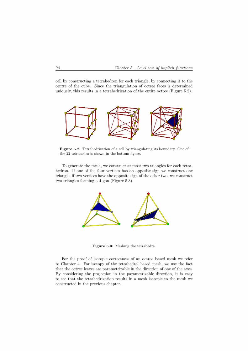
78. Chapter 5. Level sets of implicit functions

cell by constructing a tetrahedron for each triangle, by connecting it to thecentre of the cube. Since the triangulation of octree faces is determineduniquely, this results in a tetrahedrization of the entire octree (Figure 5.2).

Figure 5.2: Tetrahedrization of a cell by triangulating its boundary. One ofthe 22 tetrahedra is shown in the bottom figure.

To generate the mesh, we construct at most two triangles for each tetra-hedron. If one of the four vertices has an opposite sign we construct onetriangle, if two vertices have the opposite sign of the other two, we constructtwo triangles forming a 4-gon (Figure 5.3).

Figure 5.3: Meshing the tetrahedra.

For the proof of isotopic correctness of an octree based mesh we referto Chapter 4. For isotopy of the tetrahedral based mesh, we use the factthat the octree leaves are parametrizable in the direction of one of the axes.By considering the projection in the parametrizable direction, it is easyto see that the tetrahedrization results in a mesh isotopic to the mesh weconstructed in the previous chapter.

5.3. Level sets 79.

5.3 Level sets

In this section we shall extend the isotopic approximation algorithm to meshlevel sets of an implicit function. Changing the isovalue means that theisosurface moves through the singularities of the implicit function. Our staticalgorithm only works for regular surfaces.

For the isotopic approximation algorithm, we required as little informa-tion about the implicit function as possible. We used a black box approach,where we can only compute function values and derivatives at points andover intervals. With this approach it is not possible to determine when andwhere exactly singularities occur. Note that the surface passing through asingularity of F only depends on the value of F at that point. Higher orderderivatives do not give any more information. This implies that we wouldneed to know the exact location and function value of singularities points.With the black box approach this is not possible. However, we can constructarbitrarily small boxes around the singularities, by terminating the subdivi-sion at a predetermined maximum level. The leaves at the maximum levelfor which the gradient variation bound does not hold could contain singu-larities of the implicit function. We call these singular boxes, although theydo not necessarily have to contain a singularity of F. Outside these singularboxes the topology is already guaranteed. For the singular boxes we can testwhether θ /∈ 2F(C). If this is the case, then also inside the singular box wehave correct topology. If not, there is not much more we can do. We couldsubdivide further until the isotopy class is determined, but since we do notknow if the isosurface for the current value of θ is regular there is no guaran-tee that this process terminates. Instead, we choose to simply mark the boxas ‘red’. For visualization purposes, this means that we can easily identifyfor which isovalues we have small areas with uncertain topology. Dependingon the requirements of the user, we could choose to do further octree refine-ment, which could remove the topological uncertainty. For specific classesof surfaces, such as algebraic surfaces, we could also examine the functionitself to study the possible singularity inside a red box.

5.3.1 Algorithm

Instead of looking at the zero set F = 0 we now consider the level set F = θ.For subdivision this means we have to examine the interval condition

θ /∈ 2F(C) ∨ 〈2∇F(C),2∇F(C)〉 > 0.

The lefthand clause is dependent on the specific level set θ. We there-fore subdivide the initial octree until the righthand clause holds or until a

80. Chapter 5. Level sets of implicit functions

predetermined maximum depth is reached. For a better Hausdorff accuracywe could also perform extra subdivision until all leaves have a fixed mini-mum depth. As in the static case we balance the tree for convenience. Forthe resulting octree we precompute 2F(C) for all leaves for which the gra-dient variation bound does not hold. This way we can easily check whetherθ /∈ 2F(C), and therefore determine quickly if the topology inside a cell isguaranteed.

If we also store the function values at the octree vertices, the resultingdata structure contains all the information we need to create the meshes fordifferent level sets. Also, if the isovalue changes only by a small amount wecan locally update the mesh.

Starting with an isovalue outside the range of function values at octreevertices, the initial mesh is empty. If we change the isovalue θ, the combina-tory of the mesh only changes in cells for which θ passes the function valueof one of the vertices on the boundary of that cell. Otherwise we only haveto move existing mesh vertices to maintain linear interpolation. For the cellswhere the combinatory does change we simply remesh these octree leaves.Meshing of a single cell is done by tetrahedrizing the cell, and subsequentlymeshing the tetrahedra.

After (or during) updating the mesh, we examine all singular boxes. Re-call that these are the octree leaves of maximal depth for which the gradientvariation bound does not hold. If for such a leave θ ∈ 2F(C), we mark theleave as ‘red’. In our implementation we display small red boxes for theseleaves, indication that there is an uncertainty in topology. For nonemptyleaves having vertices with function values both larger and smaller than θ,we could also construct a local triangle mesh, displaying these triangles inanother colour to indicate the topological uncertainty.

In practice we can now move interactively through the level sets of animplicit function. For regular surfaces the mesh will be isotopic to the im-plicit surface, except for small red boxes appearing if the surface moves closeto or through a singular box of the octree. If the maximum subdivision levelis large enough, these singular boxes will only appear in the neighbourhoodof singularities of the implicit function.

After further user input we could do a temporary refinement of the octreeinside these red boxes, or perform some kind of analysis of the implicitfunction. For almost all θ the corresponding isosurface is regular, and a fewextra levels of subdivision should remove most of the red boxes.

5.4. Results 81.

5.4 Results

For the implemention we computed the tetrahedrization immediately afterbalancing of the octree. We stored the information about the implicit func-tion (such as function range, gradient variation bound and vertex values) inthe tetrahedron structure. By storing this information of the octree leavesin the tetrahedron structure, the octree itself is not needed anymore. Un-fortunately, storing the entire tetrahedrization of the octree takes up a lotof memory space, resulting in fairly low maximum subdivision levels.

We tested the implentation on several implicit functions. In this sectionwe show some results for the Tangle Cube, the Chair surface and for a non-algebraic surface (Figure 5.4).

In Figure 5.5 two isosurfaces of the tangle cube are shown. This surfaceis defined by:

F(x, y, z) = x4 − 5x2 + y4 − 5y2 + z4 − 5z2

Figure 5.6 shows a series of close-ups as the isosurface passes a singularity.With a maximum subdivision level of 9, the red boxes are small, and onlyappear when the surface is fairly close to the singular boxes. They couldeasily be removed by further subdivision, but this would require interventionof the user.

Figure 5.7 shows the ‘chair’ function:

F(x, y, z) = (x2 + y2 + z2 − ak2)2 − b((z − k)2 − 2x2)((z + k)2 − 2y2),

with k = 5, a = 0.95 and b = 0.8. Due to the higher number of com-putations, the interval arithmetic converges slower, and the bound on thevariation of the gradient is only satisfied at a higher level of subdivision.The maximum subdivision level used for Figure 5.7 is 6, resulting in largeareas of red boxes. Although they could be removed with extra subdivision,it seems that in this case a higher initial subdivision level would performbetter. However, this requires an implementation that does not store theentire tetrahedrization.

The non-algebraic surface is given by the function:

F(x, y, z) = −4 (sin(5x) + sin(5y) + cos(5z)) + x2 + 3y2 + 2z2

This surface consists of many components and passes through a lot of singu-larities. Approximation the entire surface requires a large initial subdivisionlevel. We approximated the part of the surface defined by the bounding box[2, 2.5]× [2, 2.5]× [2, 2.5] with a maximum subdivision level of 8. Results areshown in Figure 5.8, giving a good indication of the stages where red boxes

82. Chapter 5. Level sets of implicit functions

appear and disappear. Notice in particular how red boxes appear just beforea new component appears and again before it merges with the main surfacecomponent.

The timing results for the preprocessing are given in the following table.The time required for updating the mesh when the isovalue θ changes isdependent on the function and the values of the previous and new valuesfor θ. In our experiments the updating typically takes a few tenths of asecond, fast enough for interactive examination of the level sets. The tableshows the time for computing the octree and the tetrahedrization, and thesize of the octree (number of leaves), the balanced octree and the number oftetrahedra. The numbers in parentheses indicate the maximum subdivisionlevel used.

tangle (9) chair (6) non-alg. (8)Octree subdiv 0.432s 0.484s 0.468sTetrahedrization 3.036s 5.468s 6.984sOctree size 45032 66592 34987Balanced size 46544 66760 49253Tetrahedra 696432 862800 792638

Our experiments show that a maximal subdivision level of 8 or 9 re-sults in a small number of red boxes. Since the tetrahedrization uses muchmore memory than the octree, an implementation that computes the tetra-hedrization locally on demand should perform better. For small changesin the isovalue θ the number of octree leaves that require tetrahedrizationis small. Comparing the time required for complete tetrahedrization withthe size of the octree suggests that the time for updating the mesh wouldincrease only slightly.

5.5 Conclusion and future work

Depending on the specific requirements there are lots of options in imple-menting the algorithm. For example, to move through an entire range oflevel sets, we could sort the vertices of the octree on function value. Thislist can be used to determine quickly where the next combinatorial changesin the mesh will occur.

From our results it is clear that we have to make a trade-off betweenspeed and memory. Storing only the octree requires much less memoryspace, allowing a greater maximum depth of the initial tree. However, up-dating the mesh will take slightly more time due to the tetrahedrizationand recomputation of function values. Another option is to precompute thetetrahedrization, and store it in external memory.

It is not yet clear how to deal with the red boxes. The static algorithm for

5.5. Conclusion and future work 83.

implicit functions terminates fairly quickly for regular surfaces. We expectthat a few extra levels of subdivision would remove most of the red boxes.Again there is a trade-off between a lower initial subdivision combined withextra subdivision of red boxes, or starting with a higher initial subdivisionlevel.

Another open problem is whether changing from interval arithmetic toaffine arithmetic (AA) [24] will speed up the algorithm. AA computationsare slower, but the results converge faster. Another option that we used inour implementation is to use standard interval arithmetic with extra levelsof subdivision.

84. Chapter 5. Level sets of implicit functions

Figure 5.4: The tangle cube, the chair, and the non-algebraic surface.

5.5. Conclusion and future work 85.

Figure 5.5: Level sets of the tangle cube.

Figure 5.6: Close up of the ‘red’ boxes for level sets of the tangle cube. Themaximum subdivision level is 9.

86. Chapter 5. Level sets of implicit functions

Figure 5.7: Level sets of the chair, with a maximum subdivision level of 6.

5.5. Conclusion and future work 87.

Figure 5.8: Level sets of part of the non-algebraic surface, with a maximumsubdivision level of 8.

88. Chapter 5. Level sets of implicit functions

Appendix A

Singularities of functions on surfaces

A.1 Non-degenerate singular points

Consider an implicit surface S = F−1(0), where F : R3 → R is a C2 function.

We assume that 0 is a regular value of F, so according to the Implicit FunctionTheorem S is a regular C2-surface.

Our goal is to determine conditions which guarantee that the restrictionof a C2 function G : R

3 → R to the surface S has a non-degenerate singularpoint.

As for notation, the gradient of a function F : R3 → R at p ∈ R will be

denoted by ∇F(p). Furthermore, the Hessian quadratic form of a functionF : R

3 → R at p ∈ R will be denoted by HF(p). Usually, we suppress thedependence on p from our notation, and denote this quadratic form by HF.With respect to the standard euclidean inner product its matrix is the usualsymmetric matrix whose entries are the second order partial derivatives ofF. We denote partial derivatives using subscripts, e.g., Fx denotes ∂F

∂x, Fxy

denotes ∂2F∂x∂y

, etc.

Theorem 14. Let F,G : R3 → R be C2 functions, and let 0 be a regular

value of F. Let p be a point on the surface S = F−1(0).

1. p is a singular point of G|S iff there is a real number λ such that

∇G(p) = λ∇F(p). (A.1)

2. Furthermore, the singular point p is non-degenerate iff

(HG − λHF) | TpS (A.2)

is a non-degenerate quadratic form, where λ is as in (A.1).

90. Appendix A. Singularities of functions on surfaces

Remark The scalar λ in (A.1) is traditionally called a Lagrange multiplier.

Corollary 15. The singularity p of G|S is non-degenerate iff the 2×2-matrix∆, defined by (A.3), is non-singular:

∆ = VT · (

Gxx Gxy Gxz

Gxy Gyy Gyz

Gxz Gyz Gzz

− λ

Fxx Fxy FxzFxy Fyy FyzFxz Fyz Fzz

) · V, (A.3)

where λ is the Lagrange multiplier defined by (A.1), and V is a 3× 2-matrixwhose columns span the tangent space TpS. Here all first and second orderderivatives are evaluated at p. Furthermore, for G|S, the singular point p isa maximum or minimum if det(∆) > 0, and a saddle point if det(∆) < 0.

In particular, we may take V = X, V = Y, or V = Z if Fx(p) 6= 0, Fy(p) 6= 0,or, Fz(p) 6= 0, respectively, where

X =

Fy Fz−Fx 0

0 −Fx

, Y =

−Fy 0

Fx Fz0 −Fy

, Z =

−Fz 0

0 −FzFx Fy

. (A.4)

Proof of Theorem 14 1. Saying that p is a singular point of G|S isequivalent to dGp(v) = 0, for all v ∈ TpS. Since TpS = kerdFp, we see thatthis is equivalent to the existence of a scalar λ such that dGp = λdFp.

2. Since 0 is a regular value of F, we have ∇F(p) 6= 0. We assume thatFx(p) 6= 0, and argue similarly in case Fy(p) 6= 0 or Fz(p) 6= 0. Furthermore,assume that p = (0, 0, 0). According to the Implicit Function Theorem,there is a unique local solution x = f(y, z), with f(0, 0) = 0, of the equationF(x, y, z) = 0. Implicit differentiation yields

Fx fy + Fy = 0, (A.5)

Fx fz + Fz = 0, (A.6)

where fy and fz are evaluated at (y, z), and Fx, Fy and Fz are evaluated at(f(y, z), y, z). Similarly,

Fxx f2y + 2Fxyfy + Fyy + Fxfyy = 0. (A.7)

Similar identities are obtained by differentiating (A.5) with respect to y, and(A.6) with respect to z.

Using y and z as local coordinates on S, we obtain the following expres-sion of G|S with respect to these local coordinates:

g(y, z) = G(f(y, z), y, z).

A.1. Non-degenerate singular points 91.

Differentiating this identity twice with respect to y we obtain

gyy = Gxx f2y + 2Gxyfy + Gyy +Gx fyy. (A.8)

Since Fx(p) 6= 0, we solve fyy from (A.7), and plug the resulting expressioninto (A.8), to get

gyy = (Gxx − λFxx) f2y + 2(Gxy − λFxy) fy + (Gyy − λFyy), (A.9)

where

λ =Gx

Fx

is the Lagrange multiplier, cf. (A.1). We rewrite (A.9) as

gyy =(

fy 1 0)

(HG − λHF)

fy1

0

=1

F2x

(

Fy −Fx 0)

(HG − λHF)

Fy−Fx0

We similarly derive

gyz =1

F2x

(

Fy −Fx 0)

(HG − λHF)

Fz0

−Fx

,

and

gzz =1

F2x

(

Fz 0 −Fx)

(HG − λHF)

Fz0

−Fx

.

Since the vectors (Fy,−Fx, 0) and (Fz, 0,−Fx) span the tangent space TpS, wesee that

(

gyy gyzgyz gzz

)

=1

F2x∆.

92. Appendix A. Singularities of functions on surfaces

Appendix B

The Morse Lemma with parameters

The Morse Lemma gives a normal form for a smooth function in a neigh-borhood of a non-degenerate critical point. We discuss an extension of thisresult to functions depending on parameters. We refer to [4] for a proof. LetF : R

n×Rk → R be a smooth map, and let the function f : R

n → R, definedby f(x) = F(x, 0), have a non-degenerate singularity at p ∈ R

n. Then thefunction Fµ : R

n → R has a non-degenerate singularity pµ, which dependssmoothly on µ ∈ R

k, and coincides with p for µ = 0. In fact, the singularpoint x = pµ is a solution of the system of equations

∂F

∂x1(x, µ) = · · · =

∂F

∂xn(x, µ) = 0.

The Jacobian determinant of this system at (x, µ) = (p, 0) is equal to thedeterminant of the Hessian matrix of f at 0, which is non-zero. Therefore,the Implicit Function Theorem guarantees the existence and uniqueness ofthe local solution pµ.

Proposition 16. There is a local diffeomorphism Φ : Rn×R

k → Rn×R

k,defined on a neighborhood of (p, 0), of the form

Φ(x, µ) = (ϕ(x, µ), µ),

such thatF ◦Φ(x, µ) = σ1x

21 + · · · + σnx2n + F(pµ, µ),

where σi = ±1, i = 1, . . . , n, defines the signature of the quadratic part of fat p.

The proof of the Morse Lemma with parameters is completely similar tothe proof of the ‘regular’ Morse Lemma.

94. Appendix B. The Morse Lemma with parameters

Appendix C

Normal form of a Whitney fold

C.1 Fold points of good mappings

A celebrated theorem of Whitney [70] states that generic mappings of theplane into the plane have only two types of singular points, namely folds orcusps. In this section we discuss a normal form for such a mapping in theneighborhood of a fold point, and sketch a method for actually computingsuch a normal form.

Let f : R2 → R

2 be a mapping, and let J : R2 → R be its Jacobian

determinant. More precisely, if f(x, y) = (u(x, y), v(x, y)), then

J = uxvy − uyvx.

The mapping f is called good if J(p) 6= 0 or ∇J(p) 6= 0, at every point p ∈ R2.

In other words, the system of equations

J(x, y) = Jx(x, y) = Jy(x, y) = 0 (C.1)

has no solutions in R2. It can be proven that this condition is independent

of the choice of coordinates.

Whitney proves that generically a map from the plane into the plane isgood. Intuitively, this may seem to follow from the observation that genericsystems of three equations in two unknowns do not have a solution. However,it is not obvious that (C.1) is a generic system. A proof can be given usingThom’s transversality theorem.

Consequently, the singular set S1(f) = J−1(0) of a good map consists ofa number of disjoint regular curves in the plane. This is a straightforwardconsequence of the Implicit Function Theorem, since the gradient of J isnon-zero at every point of S1(f).

96. Appendix C. Normal form of a Whitney fold

Furthermore, at a singular point p at least one of the partial derivativesof the component functions of f is non-zero, i.e.

(ux(p), uy(p), vx(p), vy(p)) 6= (0, 0, 0, 0). (C.2)

In particular, the rank of the derivative dfp at a singular point is one, or,equivalently, the kernel of dfp is one-dimensional. A singular point p of agood map f is called a fold point [29] if

TpS1(f) ⊕ Kerdfp = R2. (C.3)

Note that the tangent space TpS1(f) is well-defined, since S1(f) is a regularcurve. Whitney’s version [70] of (C.3) is slightly different: if w is a non-zero tangent vector at p to S1(f), then the directional derivative of f in thedirection w is non-zero, i.e., ∇wf(p) 6= 0. Obviously, the two versions areequivalent, and, more importantly, neither version depends on a particularchoice of coordinates. The latter observation follows from Lemma 17.

Lemma 17. Let f be a good map, ϕ : R2 → R

2 an invertible non-singularmap, and g = f ◦ϕ. Then

(i) S1(g) = ϕ−1(S1(f));

(ii) g(S1(g)) = f(S1(f));

(iii) g is a good map;

(iv) p is a fold point of g iff ϕ(p) is a fold point of f.

Proof. Let J and J be the Jacobian determinants of f and g, respectively.Since

dgp = dfϕ(p) ◦ dϕp, (C.4)

we see thatJ(p) = J(ϕ(p)) · detdϕp. (C.5)

Therefore, ϕ(J−1(0)) = J−1(0), which is equivalent to first claim. The secondclaim is an immediate consequence of the first one. To prove the third claim,let p ∈ S1(g), i.e., J(p) = 0. Then (C.5) implies J(ϕ(p)) = 0. Therefore,applying the product rule to (C.5) yields

dJp = detdϕp ◦ dJϕ(p) ◦ dϕp. (C.6)

Since dϕp is invertible, we see that the scalar detdϕp is non-zero, and hencethat

dJp 6= 0 iff dJϕ(p) 6= 0.

C.1. Fold points of good mappings 97.

This proves the third claim. Finally, observe that (C.4) implies

dϕp(Kerdgp) = Kerdfϕ(p), (C.7)

and that (C.6) implies

dϕp(KerdJp) = KerdJϕ(p). (C.8)

Since KerdJp = TpS1(g), and KerdJϕ(p) = Tϕ(p)S1(f), we conclude from(C.7) and (C.8) that

TpS1(g) ⊕ Kerdgp = R2 iff Tϕ(p)S1(f) ⊕ Kerdfϕ(p) = R

2,

in other words: p is a fold point of g iff ϕ(p) is a fold point of f. Thisconcludes the proof of the fourth claim.

For later use, we isolate the following result.

Lemma 18. Let f : R2 → R

2 be a good map, with component functionsu, v : R

2 → R, and Jacobian determinant J : R2 → R. The following

statements are equivalent:

(i) p is a fold point of f;

(ii) Wp 6= (0, 0), where

Wp = (〈∇u(p),∇J(p)⊥〉, 〈∇v(p),∇J(p)⊥〉).

In either case, Wp is a tangent vector of the regular curve f(S1(f)) at p.

Proof. Since f is good, J−1(0) = S1(f) is a regular curve, containing p. Itstangent vector at p is ∇J(p)⊥.

Since dfp has rank one, we have ∇u(p) 6= (0, 0) or ∇v(p) 6= (0, 0).Assume the former inequality holds. Then there is a real constant c suchthat

∇v(p) = c∇u(p).

Nowdfp(W) = (〈∇u(p),W〉, 〈∇v(p),W〉), (C.9)

for W ∈ R2, so dfp(∇u(p)⊥) = (0, 0). Hence Kerdfp = R∇u(p)⊥.It now follows that (C.3) is holds iff ∇u(p)⊥ is not parallel to ∇J(p)⊥, or,

iff 〈∇u(p),∇J(p)⊥〉 6= 0. Similarly, if ∇v(p) 6= 0, then (C.3) is equivalent to〈∇v(p),∇J(p)⊥〉 6= 0. In either case, Wp 6= 0. This proves the equivalenceof (i) and (ii).

98. Appendix C. Normal form of a Whitney fold

To prove that Wp is tangent to f(S1(f)) at p, let s 7→ (x(s), y(s)) be aregular parametrization of J−1(0), with (x(0), y(0)) = p, and (x ′(0), y ′(0)) =

∇J(p)⊥. Then α(s) = f(x(s), y(s)) is a parametrization of f(J−1(0)), and, inview of (C.9 we have

α ′(0) = dfp(∇J(p)⊥) = Wp. (C.10)

C.2 Normal form of a good map near a fold

point

Our goal is to obtain a simple form of a good map near a fold point. Sucha normal form can be obtained by applying a change of coordinates on thedomain of the map, on its range, or both. We start by applying only changesof coordinates on the domain of the map.

Proposition 19. Let f : R2 → R

2 be a good map with component functionsu, v : R

2 → R, and Jacobian determinant J : R2 → R. Let p = (0, 0) be a

fold point of f, with f(p) = (0, 0). The following properties are equivalent:

(i) f(J−1(0)) is transversal to the y-axis at f(p);

(ii) ∇u(p) 6= (0, 0);

(iii) There is a local change of coordinates ϕ : R2 → R

2, with ϕ(0, 0) = p,such that

f ◦ϕ(x, y) = (x, σy2 + α(x)), (C.11)

where σ = sign(〈∇u(p),∇J(p)⊥〉) = ±1, and α : R → R is a smoothfunction with α(0) = 0.

Remark 20. If g = f◦ϕ, we shall say that ϕ brings f into the form g. Theright hand side of (C.11) will be considered as a normal form. The transfor-mations bringing the mapping into normal form should be computationallyfeasible. Therefore, we shall be very precise about each and every step wetake.

Proof. of Proposition 19The equivalence of conditions (i) and (ii) follows from Lemma 18. To seethat (iii) implies (i), let g = f ◦ ϕ, then f(S1(f)) = g(S1(g)), according toLemma 17.(ii). Since g(S1(g)) = {(x, α(x)) | x ∈ R

2}, the first claim follows.

C.2. Normal form of a good map near a fold point 99.

So it remains to prove that the (ii) implies (iii). The proof goes in two steps.We assume that p = (0, 0).Step 1. There is a local change of coordinates bringing f into one of theforms g(x, y) = (x, V(x, y)).To see this, we first consider the case

u0x 6= 0, (C.12)

where the notation is as in Section C.1. Here the superscript 0 indicatesthat the corresponding function has to be evaluated at p = (0, 0) ∈ R

2. Inview of (C.12), the change of coordinates ψ : R

2 → R2, defined by

ψ(x, y) = (u(x, y), y),

is non-singular. Let ϕ be the inverse of ψ, then ϕ(x, y) = (ξ, η) iff η = y

andu(ξ, y) − x = 0. (C.13)

Let ξ = ξ(x, y) be the locally unique solution of (C.13) with ξ(0, 0) = 0,then

ϕ(x, y) = (ξ(x, y), y),

andf ◦ϕ(x, y) = (x, V(x, y)), with V(x, y) = v(ξ(x, y), y).

If u0x = 0, then condition (ii) implies that u0y 6= 0. This case is reduced to(C.12) by first applying the transformation (x, y) 7→ (y, x).

Step 2. If f(x, y) = (x, V(x, y)) is a good map with a fold point at (0, 0),then there is a local change of coordinates bringing g into the form g(x, y) =

(x,±y2 + α(x)), where α : R → R is a smooth function with α(0) = 0.

Since

df(x,y) =

(

1 0

Vx Vy

)

,

we see that (0, 0) is a singular point of f iff

V0y = 0. (C.14)

In that case, Kerdf(0,0) is the span of the vector (0, 1). Furthermore, J = Vy,so the fact that f is a good mapping implies in particular that ∇J(0, 0) =

(V0xy, V0yy) 6= (0, 0). A non-zero tangent vector to S1(f) = J−1(0) at (0, 0)

is ∇J(0, 0)⊥ = (−V0yy, V0xy). It is now easy to see that condition (C.3) is

equivalent toV0yy 6= 0. (C.15)

100. Appendix C. Normal form of a Whitney fold

Since also V(0, 0) = 0, we apply the Morse Lemma with parameters to bringthe function V into normal form. More precisely, there is a local change ofparameters ϕ : R

2 → R2 of the form ϕ(x, y) = (x,Φ(x, y)), such that

V ◦ϕ(x, y) = ±y2 + α(x),

where α is a smooth function with α(0) = 0. It is now obvious that f ◦ϕ isthe desired normal form.

Concatenating steps 1 and 2 concludes the proof.

Corollary 21. If f : R2 → R

2 is a good mapping with a fold point atp, then there is a local change of coordinates ϕ : R

2 → R2, near (0, 0),

with ϕ(0, 0) = p, and a local change of coordinates ψ : R2 → R

2, withψ(f(p)) = (0, 0), such that

ψ ◦ f ◦ϕ(x, y) = (x, y2).

Proof. Applying Proposition 19, we may assume that f(x, y) = (x,±y2 +

α(x)) or f(x, y) = (±x2+α(y), y). In the first case, take ψ(x, y) = (x,±(y−

α(x))). Then ψ ◦ f(x, y) = (x, y2). The second case is treated similarly.

Remark 22. In Step 1 of the proof of Proposition 19, in case ux 6= 0,near p = (0, 0), we define the function V by V(x, y) = v(ξ(x, y), y), whereξ = ξ(x, y) is the solution of u(ξ, y) − x = 0. The derivatives Vy and Vyycan be computed from this definition in a straightforward way:

Vy = vxξy + vy = vx(−uy

ux) + vy =

J

ux,

where all functions in the right hand sides are evaluated at (ξ(x, y), y). SinceJ(0, 0) = 0, we obtain

Vyy(0, 0) =(J0xξ

0y + J0y)u

0x

(u0x)2

=−u0yJ

0x + u0xJ

0y

(u0x)2

.

Therefore, Vyy(0, 0) 6= 0 iff 〈∇u(0, 0),∇J(0, 0)⊥〉 6= 0 iff the vectors ∇u(0, 0)⊥

and ∇J(0, 0)⊥ are not parallel.We claim that ∇u(0, 0)⊥ = (−u0y, u

0x) is a non-zero vector in Kerdf0.

Indeed, since df0 has rank 1, we see that ∇v(0, 0) = c∇u(0, 0), for some realconstant c. Therefore

(

u0x u0yv0x v0y

)(

−u0yu0x

)

=

(

0

0

)

,

C.3. Introducing parameters 101.

which proves our claim. Since ∇J(0, 0)⊥ is tangent to J−1(0) = S1(f), we seethat the latter condition is equivalent to (C.3). In other words: Vyy(0, 0) 6= 0

iff condition (C.3) holds. This is what we also observed in Step 2 of the proofof Proposition 19.

C.3 Introducing parameters

If f depends on an additional parameter t, we can still obtain a normal formlike (C.11), provided we let both the transformation ϕ and the function αdepend on this new parameter. More precisely, consider a family of mapsft : R

2 → R2, depending smoothly on the parameter t ∈ R, such that f0

satisfies any of the conditions (i), (ii) and (iii) of Proposition 19. With thisfamily we associate the map F : R

2 × R → R2, defined by F(x, t) = ft(x).

Then there is a one-parameter familyΦ : R2×R → R

2×R of local coordinatetransformations of the form

Φ(x, y, t) = (ϕt(x, y), t),

such thatF ◦Φ(x, y, t) = (x, σy2 + α(x, t)). (C.16)

The latter identity may be rephrased as

ft ◦ϕt(x, y) = (x, σy2 + α(x, t)).

The image of the fold curve of ft is ft(S1(ft)) = {(x, α(x, t)) | x ∈ R}. Thepoint of intersection of this curve with the y-axis, viz (0, α(0, t)), passesthrough the origin with speed α0t (Here we consider t as time) . To expressthis velocity in terms of ft, let u(x, y, t) and v(x, y, t) be the componentfunctions of F(x, y, t).

Lemma 23. If ux(p, 0) 6= 0, then

α0t =1

ux(p, 0)

∂(u, v)

∂(x, t)(p, 0),

and if uy(p, 0) 6= 0, then

α0t =1

uy(p, 0)

∂(u, v)

∂(y, t)(p, 0).

Proof. Let Φ(x, y, t) = (ξ(x, y, t), η(x, y, t)). Then (C.16) boils down to

u(ξ(x, y, t), η(x, y, t), t) = x,

v(ξ(x, y, t), η(x, y, t), t) = σy2 + α(x, t).

102. Appendix C. Normal form of a Whitney fold

Differentiating the latter identity with respect to t and evaluating at (p, 0)

yields

u0xξ0t + u0yη

0t + u0t = 0,

v0xξ0t + v0yη

0t + v0t = α0t .

(C.17)

Since the second condition of Proposition 19 holds, i.e., (u0x, u0y) 6= (0, 0),

there is a scalar constant c such that (u0x, u0y) = c(v0x, v

0y). Therefore, (C.17)

implies:

α0t = v0t − cu0t =1

u0x(u0xv

0t − v0xu

0t ).

If u0y 6= 0, the second identity is derived similarly.

Remark 24. Lemma 23 implies that α0t 6= 0 iff the matrix

(

u0x u0y u0t

v0x v0y v0t

)

has rank two. Furthermore, since u0xv0y − u0yv

0x = 0, it follows that

u0y

∣

∣

∣

∣

u0x u0tv0x v0t

∣

∣

∣

∣

= u0x

∣

∣

∣

∣

u0y u0tv0y v0t

∣

∣

∣

∣

.

In view of Lemma 23 both sides of this equality are equal to u0xu0yα0t .

Bibliography

[1] Samir Akkouche and Eric Galin. Adaptive implicit surface polygoniza-tion using marching triangles. In D. Duke and R. Scopigno, editors,Computer Graphics Forum, volume 20(2), pages 67–80. Blackwell Pub-lishing, 2001. [6, 54]

[2] L. Alberti, G. Compte, and B. Mourrain. Meshing implicit algebraicsurfaces: the smooth case. Technical Report TR. 5405, INRIA Sophia-Antipolis, December 2004. [44]

[3] P. Alliez, N. Laurent, H. Sanson, and et al. Efficient view-dependentrefinement of 3D meshes using sqrt3-subdivision. In The Visual Com-puter, volume 19(4), pages 205–221. Springer, July 2003. [5, 15]

[4] V.I. Arnol’d. Wave front evolution and equivariant morse lemma.Comm. Pure Appl. Math., 29:557–582, 1976. [16, 93]

[5] V.I. Arnol’d. Catastrophe Theory. Springer-Verlag, 1986. [16]

[6] Koji Ashida. Adaptive construction of manifold meshes. PhD thesis,University of Pennsylvania, 2003. [7]

[7] Koji Ashida and Norman I. Badler. Feature preserving manifold meshfrom an octree. In SM ’03: Proceedings of the eighth ACM symposiumon Solid modeling and applications, pages 292–297, New York, NY,USA, 2003. ACM Press. [7]

[8] G. Barequet, C.A. Duncan, M.T. Goodrich, S. Kumar, and M. Pop.Efficient perspective-accurate silhouette computation. In Proc. 15thAnnu. ACM Sympos. Comput. Geom., pages 417–418, 1999. [16]

[9] J. Bloomenthal. Introduction to Implicit Surfaces. Morgan-Kaufmann,1973. [16]

104. Bibliography

[10] Jules Bloomenthal. Polygonization of implicit surfaces. Computer AidedGeometric Design, 5:341–355, 1988. [7, 54]

[11] Jules Bloomenthal and Ken Shoemake. Convolution surfaces. In SIG-GRAPH ’91: Proceedings of the 18th annual conference on Computergraphics and interactive techniques, pages 251–256, New York, NY,USA, 1991. ACM Press. [3]

[12] J. Boissonnat and S. Oudot. Provably good surface sampling and ap-proximation, 2003. [8]

[13] J.D. Boissonnat, D. Cohen-Steiner, and G. Vegter. Isotopic implicitsurface meshing. In Proceedings Thirty-Sixth Annual ACM Symposiumon Theory of Computing, Chicago, 2004. [12, 54, 75]

[14] J.D. Boissonnat and S. Oudot. An effective condition for samplingsurfaces with guarantees. In Proceedings ACM Symposium on SolidModeling, 2004. [54, 76]

[15] A. Bottino, W. Nuij, and K. van Overveld. How to shrinkwrap through acritical point: an algorithm for the adaptive triangulation of iso-surfaceswith arbitrary topology. In Proc. Implicit Surfaces, pages 55–72, 1996.[54, 75]

[16] David Bremer and John F. Hughes. Rapid approximate silhouette ren-dering of implicit surfaces. In Proc. Implicit Surfaces, 1998. [5, 15,53]

[17] J.W. Bruce. Seeing – the mathematical viewpoint. The MathematicalIntelligencer, 6:18–25, 1984. [16]

[18] J.W. Bruce and P.J. Giblin. Outlines and their duals. Proc. LondonMath. Soc. (3), 50:552–570, 1985. [16]

[19] J. C. Carr, R. K. Beatson, J. B. Cherrie, T. J. Mitchell, W. R. Fright,B. C. McCallum, and T. R. Evans. Reconstruction and representation of3d objects with radial basis functions. In SIGGRAPH ’01: Proceedingsof the 28th annual conference on Computer graphics and interactivetechniques, pages 67–76, New York, NY, USA, 2001. ACM Press. [4]

[20] Martin Cermak and Vaclav Skala. Adaptive edge spinning algorithmfor poligonization of implicit surfaces. In CGI ’04: Proceedings of theComputer Graphics International (CGI’04), pages 36–43, Washington,DC, USA, 2004. IEEE Computer Society. [6]

Bibliography 105.

[21] S.W. Cheng, T.K. Dey, E.A. Ramos, and T.Ray. Sampling and mesh-ing a surface with guaranteed topology and geometry. In ProceedingsSymposium on Computational Geometry, 2004. [54, 76]

[22] Evgeni V. Chernyaev. Marching cubes 33: Construction of topologicallycorrect isosurfaces. Technical Report CERN CN 95–17, 1995. [6, 54]

[23] R. Cipolla and P.J. Giblin. Visual Motion of Curves and Surfaces.Cambridge University Press, 2000. [16]

[24] J. L. D. Comba and J. Stolfi. Affine arithmetic and its applicationsto computer graphics. In Proc. VI Brazilian Symposium on ComputerGraphics and Image Processing (SIBGRAPI’93), pages 9–18, 1993. [10,83]

[25] Erwin de Groot and Brian Wyvill. Rayskip: faster ray tracing of implicitsurface animations. In GRAPHITE ’05: Proceedings of the 3rd inter-national conference on Computer graphics and interactive techniques inAustralasia and South East Asia, pages 31–36, New York, NY, USA,2005. ACM Press. [1]

[26] Mathieu Desbrun and Marie-Paule Cani. Active implicit surface foranimation. In Graphics Interface, pages 143–150, Jun 1998. Publishedunder the name Marie-Paule Cani-Gascuel. [1]

[27] Mathieu Desbrun and Marie-Paule Gascuel. Animating soft substanceswith implicit surfaces. In SIGGRAPH ’95: Proceedings of the 22nd an-nual conference on Computer graphics and interactive techniques, pages287–290, New York, NY, USA, 1995. ACM Press. [1]

[28] A.T. Fomenko and T.L. Kunii. Topological Modeling for Visualization.Springer-Verlag, 1997. [23]

[29] M. Golubitsky and V. Guillemin. Stable Mappings and Their Singu-larities, volume 14 of Graduate Texts in Mathematics. Springer-Verlag,1973. [96]

[30] T. Greg and J. O’Brien. Variational implicit surfaces, 1999. [4]

[31] X. Gu, S.J. Gortler, H. Hoppe, L. McMillan, B.J. Brown, and A.D.Stone. Silhouette mapping. Technical Report TR-1-99, Harvard Uni-versity, March 1999. [16]

[32] E.R. Hansen and R.I. Greenberg. An interval newton method. AppliedMathematics and Computation, 12:89–98, 1983. [10]

106. Bibliography

[33] John C. Hart. Ray tracing implicit surfaces. In SIGGRAPH 93 Mod-eling, Visualizing, and Animating Implicit Surfaces course notes, pages13–1 to 13–15. 1993. [1]

[34] John C. Hart. Sphere tracing: Simple robust antialiased rendering ofdistance-based implicit surfaces. In SIGGRAPH 93 Modeling, Visualiz-ing, and Animating Implicit Surfaces course notes, pages 14–1 to 14–11.1993. [1]

[35] Erich Hartmann. A marching method for the triangulation of surfaces.The Visual Computer, 14(3):95–108, 1998. [6, 53]

[36] D. Hearn and M.P. Baker. Computer Graphics, 2nd edition. Prentice-Hall, 1994. [22]

[37] Aaron Hertzmann and Denis Zorin. Illustrating smooth surfaces. InKurt Akeley, editor, Siggraph 2000, Computer Graphics Proceedings,pages 517–526. ACM Press / ACM SIGGRAPH / Addison WesleyLongman, 2000. [5]

[38] Chien-Chang Ho, Fu-Che Wu, Bing-Yu Chen, Yung-Yu Chuang, andMing Ouhyoung. Cubical marching squares: Adaptive feature preserv-ing surface extraction from volume data. Computer Graphics Forum,24(3):537–545, August 2005. Special issue: Proceedings of EURO-GRAPHICS 2005. [7]

[39] Christoph M. Hoffman. Implicit curves and surfaces in cagd. IEEEComput. Graph. Appl., 13(1):79–88, 1993. [1]

[40] K.C. Hui and Z.H. Jiang. Tetrahedra based adaptive polygonisation ofimplicit surface patches. Computer Graphics Forum, 18(1):57–68, 1999.[7]

[41] Tao Ju, Frank Losasso, Scott Schaefer, and Joe Warren. Dual contour-ing of hermite data. In SIGGRAPH ’02: Proceedings of the 29th annualconference on Computer graphics and interactive techniques, pages 339–346, New York, NY, USA, 2002. ACM Press. [7]

[42] Tasso Karkanis and A. James Stewart. High quality, curvature depen-dent triangulation of implicit surfaces. [6]

[43] Michael Kazhdan, Matthew Bolitho, and Hugues Hoppe. Poisson sur-face reconstruction. In Eurographics symposium on geometry processing,2006. [4]

Bibliography 107.

[44] J.J. Koenderink. Solid Shape. MIT-Press, 1990. [16]

[45] Nikita Kojekine, Vladimir Savchenko, and Ichiro Hagiwara. Surfacereconstruction based on compactly supported radial basis functions.pages 218–231, 2004. [4]

[46] A. Lopes and K. Brodlie. Improving the robustness and accuracy of themarching cubes algorithm for isosurfacing, 2002. [6]

[47] Adriano Martins Lopes. Accuracy in Scientific Visualization. PhDthesis, University of Leeds, 1999. [1]

[48] H. Lopes, J. B. Oliveira, and L. H. de Figueiredo. Robust adaptivepolygonal approximation of implicit curves. Computers and Graphics,26(6):841–852, 2002. [53]

[49] William E. Lorensen and Harvey E. Cline. Marching cubes: A high reso-lution 3d surface construction algorithm. In Proceedings of the 14th an-nual conference on Computer graphics and interactive techniques, pages163–169. ACM Press, 1987. [6, 54, 60]

[50] L. Markosian, M.A. Kowalski, S.J. Trychin, L.D. Bourdev, D. Goldstein,and J.F. Hughes. Real-time nonphotorealistic rendering. In SIGGRAPHProceedings, pages 415–420, 1997. [5, 15]

[51] Cermak Martin and Skala Vaclav. Polygonization by the edge spinning.In Algoritmy 2002, pages 245–252, Slovakia, 2002. Univ.of Technology.[6]

[52] J. Milnor. Morse Theory. Princeton University Press, 1963. [23]

[53] Ramon E. Moore. Interval analysis. Prentice Hall, 1966. [9]

[54] Xinlai Ni, Michael Garland, and John C. Hart. Fair morse functionsfor extracting the topological structure of a surface mesh. ACM Trans.Graph., 23(3):613–622, 2004. [12]

[55] Paul Ning and Jules Bloomenthal. An evaluation of implicit surfacetilers. IEEE Computer Graphics and Applications, 13(6):33–41, 1993.[6]

[56] University of Wuppertal. C-xsc class library. http://www.math.uni-wuppertal.de/˜xsc/. [46]

[57] A. Opalach and S. Maddock. An overview of implicit surfaces, 1995.[16]

108. Bibliography

[58] A. Opalach and S. C. Maddock. Disney effects using implicit surfaces. InProc. 5th Eurographics Workshop on Animation and Simulation, 1994.[1]

[59] Simon Plantinga and Gert Vegter. Contour generators of evolving im-plicit surfaces. In Proceedings of the eighth ACM symposium on Solidmodeling and applications, pages 23–32. ACM Press, 2003. [53]

[60] H. Ratschek and J. Rokne. Geometric computations with interval andnew robust methods. Horwood Publishing, 2003. [10]

[61] William J. Schroeder, Berk Geveci, and Mathieu Malaterre. Compatibletriangulations of spatial decompositions. In VIS ’04: Proceedings of theconference on Visualization ’04, pages 211–218, Washington, DC, USA,2004. IEEE Computer Society. [7]

[62] J.M. Snyder. Interval analysis for computer graphics. In SIGGRAPHProceedings, pages 121–130, 1992. [10]

[63] John M. Snyder. Interval analysis for computer graphics. ComputerGraphics, 26(2):121–130, 1992. [53]

[64] Barton T. Stander and John C. Hart. Guaranteeing the topology of animplicit surface polygonization for interactive modeling. In Proceedingsof the 24th annual conference on Computer graphics and interactivetechniques, pages 279–286. ACM Press/Addison-Wesley Publishing Co.,1997. [54, 75]

[65] B.T. Stander and J.C. Hart. Guaranteeing the topology of an implicitsurface polygonization for interactive modeling. In SIGGRAPH Pro-ceedings, pages 279–286, 1997. [10, 18]

[66] J. Stolfi and L. de Figueiredo. Self-Validated Numerical Methods andApplications. Institute for Pure and Applied Mathematics (IMPA),Rio de Janeiro, 1997. Monograph for the 21st Brazilian MathematicsColloquium (CBM’97), IMPA. [10]

[67] G. M. Treece, R. W. Prager, and A. H. Gee. Regularised marchingtetrahedra: improved iso-surface extraction. Computers and Graphics,23(4):583–598, 1999. [7]

[68] Greg Turk and James F. O’brien. Modelling with implicit surfaces thatinterpolate. ACM Trans. Graph., 21(4):855–873, 2002. [4]

Bibliography 109.

[69] C.W.A.M. van Overveld and B. Wywill. Shrinkwrap: An adaptive algo-rithm for polygonizing an implicit surface. Technical Report 93/514/19,University of Calgary, March 1993. [54]

[70] H. Whitney. On singularities of mappings of euclidean spaces I, map-pings of the plane into the plane. Ann. of Math., 62:374–410, 1955. [28,33, 95, 96]

[71] Andrew P. Witkin and Paul S. Heckbert. Using particles to sample andcontrol implicit surfaces. Computer Graphics, 28(Annual ConferenceSeries):269–277, 1994. [2]

[72] S. Wu, M. de, and G. Malheiros. On improving the search for criticalpoints of implicit functions, 1999. [12]

[73] Dan X. Yang. Mesh generation and information model for device sim-ulation. PhD thesis, Stanford University, 1994. [7]

[74] G. Yngve and G. Turk. Robust creation of implicit surfaces from polyg-onal meshes, 2002. [4]