Embed Size (px)
Citation preview

CERTAIN DATAcONTAiNEDIN THISDOCUMENTMAYBEDIFFICULTTOREAD
IN 'MICROFICHEPRODUCTS.

UCRL-MA--105259
DE91 007594
• DYNA3D Example Problem Manual
Steven C. LovejoyRobert G. Whirley
University of CaliforniaLawrence Livermore National LaboratoryZ
October 10, 1990
I Work performed under the auspic,_s of the U.S. Department of Energy by t1_e
" MASIELawrence Livermore National Labo atory under contract W-/405-Eng-4 . _t ._ ,, O
DISTRIBUTION OF THIS DOCUMENT 18 UNLIMITED _'j"
Contents
ABSTRACT........................................................................................................................ 7
CHAFFER1: IMIRODUCTION................................ ..... ,............................................................ 8
CHAFFER2: BAR IMPACTINGA RIGID WALL (FILE: D3SAMPI) ................................... ]0
CHAFrER3: IMPACTOF A CYLINDERINTO A RAIL (FILE: D3SAMP2) .......................... 21
CHAFFER 4: IMPACT OF TWO ELASTICSOLIDS(FILE:D3SAMP3)...................................32
CHAFFER 5: SQUARE PLATE IMPACTED BY A ROD (FILE:D3SAMP4)............................40
CHAFFER6: BOX BEAM BUCKLING(FILE: D3SAMPS)...................................................... 54
7" SPACE FRAME IMPACt (FILE: D3SAMP6)....................... ,............................ 65
CHAPTER g: THIN BEAM SUBJECTED TO AN IMPACT (FILE:D3SAMP7).........................77
t
CHAPTER 9: IMPACt ON A CYLINDRICAL SIIFA.L('b'K_: (D3SAMPS)............................89
CHAPTh_ I0: SIMPLY SUPPORTEDFLAT PLATE (FILE: D3SAMPg) ............................... 101
CHAPTER II- HOURGLASS]NO OF SIMPLY SUPPORTED PLATE (FILE:D3SAMPI0).....109
a,o_.,,s,,.lee eoooe ,l_ol,, ooolooooo oolooeoeooeeeoooooeoo oeeet, olo,.o,,ooeoeoe,,,,,, _,,,eoo.,oo,.e,.le,Do,.¢_ .,oo,.ost,,oee
J
_N C"F_....... ..................................................................................................................... ! 19o

List of FiguresFigure 2.1 Initial fiait© element mesh of quarter symmetry model ........... ,............. 13
Figm_ 2.2 Time sequence of deformation ..................................................................... 14u
Figm_ 2.3 Kiaimatic _spon_ of node 74. .................................................... ................. 16
, Figure 2.4 Time sequence of effective plastic strain contours .................................. 17
Figure 3.1 Drawing of cylinder and rail ....... .................................. ....... ....................... 0.3
Figure 3.2 Finite element mesh.................. ....... ..................... ,........................................ _24
Figure 3.3 Time sequence of deforming mesh ....................... ,.................................. ....24
Figure 3.4 Time history of support ring y-displacement ............................................ 27
Figure 3.5 Time history of dent depth-".................................................................... ....... 27
Figure 3.6 Contours of effective plastic strain at t= 6.4 ms.., .... .................... '............ 28
Figure 4.1 Finite element mesh of bar impact model ......... . ......................................... 35
Figure 4.2 X-velocity of nodes 405 and 1......................................................................... 35
Figure 4.3 Relative displacement of nodes 1 and 405 ....................................... ............ 36
Figure 4.4 Total x-displacements of nodes .405 and 1.................................................... 36
Figure 4.5 X-velocity of nodes 205 and 405 ............................................................... ,.....37
Figure 4.6 X-velocity of nodes 1 and 201 .............. ........................................................... 37
Pigurc 5.1 P'mitc clement mesh........................ ,............................................................... 44
FilpJrc 5.2 Time sequence of deformation ..................................................................... .45
, Figure 5.3 Velocity time history ............... .,.................................................................... .48
Figure _.4 Displacement time history .................. ,.......................................................... 48
" Figure 5.5 Gap time history...... ,......... ............................................................................ .49
l=igurc 5.6 Contours oi"z-displacement ........................................................................... 49
Figure 5.7 Contours of effective plastic strain............................................................. .50
Figure 5.8 Contours of effective stress .......................................................................... .50

Figure 6.1 Finite element mesh showing boundary conditions ............................... .59
Figure 6.2 Time sequence of mesh deformation ................... '....................................... 60
Figure 6.3 Z-displacement _fter buckling ............... ,...................................................... 62
Figure 7.1 Initial f'mite element mesh .......................................................................... 68
Figure 7.2 Time sequence of deforming mesh ..................................... ,........................ 69
Figure 7.3 Time historyof impacting mass z-displacement ........................................ 71 t
Figure 7.4 Time history of node 54 z-displacement ..... ................................................. 71
Figure 7.5 FA'fective stress contoms of plate at t = 5.75 X 10"4 .................................... 72
Figure 8.1 Finite element mesh .......... ,...................................................................... ....... "/9
Figure 8.2 Mesh deformation sequence .................. ...... ......... 80
Figure 8.3 Kinematic responses of node 19 ............................................................. ,...... 82
Figure 8.4 Magnified deformed mesh plots at t _ 0.9 ms and t = 1,4 ms .......... ............. 83
Figure 8.5 Effective stress and effective plastic strain of element 9bottom surface ........................................................ .......................................... 84
Figure 8.6 Effective stress and effective plastic strain of element 9mid-plane ......................................................................................................... 85
Figure 8.7 Effective stress and effective plastic strain of element 9top surface ....................................................................................................... 86
Figure 9.1 Initial finite element mesh ........................................................................... 91
Figure 9.2 T_me sequence of mesh deformation ....................................... .................... 92
Figure 9.3 Kinematic response time histories of center node ................................... 94
Figure 9.4 Contours of y-displacement .................. , ........................................................ 95
Figure 9.5 Effective stress and effective plastic strain of contours ofinner integration point .......................................................... ....................... 96
Figure 9.6 Effective stress and effective plastic strain of contours ofmiddle integration point ............................................................................... 97
Figure 9.7 Effective stress and effective plastic, strain of contours ofouter integration point .................................................................................. 98
Figure 10.1 Initial finite clement mesh of plate ........................................................... 103
Figure 10.2 Kinematic response of node 1 ..................................................................... 104
4
Figure 10.3 Time history of Oxx in element 1................................................................ 105
Figure 10.4 Contours of z-displacement at t = 0.55 ms .................................................. 105
Figure 10.5 Contours of Oxx upper, middle, and lower quadrature pointsat t = 0.55 ms ..., .......... ,.......................................... ,...... .................................... 106
Figure I1.I Example meshes with and without hourglassing .................................... 112w,
Figure 11.2 Kinematic response time histories of node 1 .............. '............. '.............. 113
Figure 11.3 Time history of Oxx in element 1 ...................... ,......................................... 114
Figure 11.4 Contours of z-displacement at t = 0.55 ms..., .............................................. 1 14
Figure 11.5 Contours of Oxx at t = 0.55 ms, ....................................................................... 115

List of Tables
Table I.I Execution Times for Ten Sample DYHA3D Problems ...................9
Table 2.1 Material Properties ............................................................................. 1 1L
Table 3.1 Material Properties... ............................................................................. 234
Table 5.1 Material Properties ............................................................................. 43
Table 6.1 Material Properties ............................. ,...................................... 5 8
Table 7.1 Material Properties.. ....................................................... , ............ 66
Table 8.1 Material properties. ................................................................................ 7 8
Table 9.1 Material Properties ................................................................................. 90
Table 10.I Material Properties ............................................................................... I01

DYNA3D Example Problem Manual
Steve C. Lovejoy
Robert G. Whirley
Applied Mechanics Group
" Methods Development GroupMechanical Engineering
October 10, 1990
Abstract
This manual describes in detail the solution of ten example problems
using the explicit nonlinear finite element code DYNA3D. The sample
problems include solid, shell, and beam element types, and a variety of
linear and nonlinear material models. For each example, there is first anengineering description of the physical problem to be studied. Next, the
analytical techniques incorporated in the model are discussed and key '
features of DYNA3D are highlighted. INGRID commands used to generate
the mesh are listed, and sample plots from the DYNA3D analysis are given.
Finally, there is a description of the TAURUS post-processing commands
used to generate the plots of the solution. This set of example problems isuseful in verifying the installation of DYNA3D on a new computer system.
" In addition, these documented analyses illustrate the application of
DYNA3D to a variety of engineering problems, and thus this manual should
be helpful to new analysts getting started with DYNA3D.i

Chapter 1Introduction
DYNA3D [1] is an explicit nonlinear finite element code for analyzing
the dynamic response of solids and structures. DYNA3D was originally
developed by John Hallquist, and is now under continuous development inthe Methods Development Group at Lawrence Livermore NationalLaboratory. lt contains a variety of beam and shell structural elements in
addition to the standard 8-node brick continuum element. A large
material library containing over 32 material models allows a wide range of
options in modeling material stress-strain behavior. Ten types of sliding
surfaces permit flexibility in modeling contact, including high pressure
interfaces and sliding friction effects. Fully vectorized coding allows
DYNA3D to take maximum advantage of computer hardware to produce '
accurate solutions at minimum cost. DYNA3D is fully operational on CRAY,
VAX, and SUN computers, and has been successfully installed on a wide
variety of other mSchines. DYNA3D has been successfully applied to a
wide range of dynamic problems including crashworthiness studies, impact
calculations, sbeet metal forming analyses, and _ordinance design,
This manual describes the application of DYNA3D to ten sample
engineering analyses, ranging from very simple to very complex. These
problems have been chosen to illustrate both modeling techniques andDYNA3D features. Each of the following chapters focuses on a different
problem to be studied. First, an engineering description of the physical
problem is given. Next, the analytical techniques incorporated in the
model are discussed, including salient features of DYNA3D use _ in the
model. Comments are give_n on alternate modeling strategies that might
have been used to achieve the same results. INGRID [2,3,4,5] pre-
processing commands required to generate the mesh are listed. To depict
the DYNA3D analysis results, each chapter concludes with sample plots and
a description of the TAURUS [6] pest-processing commands used to
generate these plots.
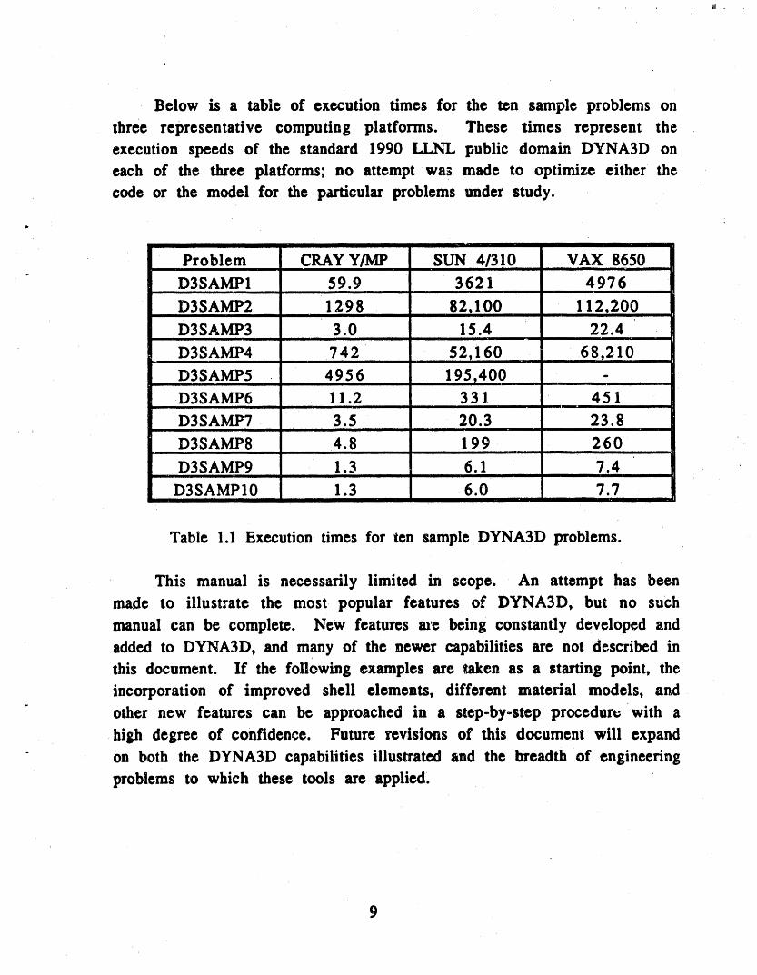
Below is a table of execution times for the ten sample problems on
three representative computing platforms. These times represent theexecution speeds of the standard 1990 LLNL public domain DYNA3D oneach of the three platforms; no attempt was made to optimize either thecode or the model for the particular problems under study.
#,
Problem CRAY Y/MP SUN 4/3 ,I0 VAX 8650l l li l ii Iii li I
D3SAMP1 59.9 3621 4976i i i ii
D3SAMP2 1298 .. 82,100 112,200iii i i
D3SAMP3 3.0 15.4 22.4iii i ii iiiii i i
D3SAMP4 74 2 .52,160 68,2! 0D3SAMP5 4956 195,400 -iii ii i illl
D3SAMP6 11.2 331 4 51iii [i l iiii J
D3SAMP7 3.5 20.3 23.8I i
D3SAMP8 4.8 199 260i i ii. iii i i
D3SAMP9 1.3 6.1 7.4ii ii i ii
D3SAMP10 1.3 6.0 7.7i i i
Table 1.1 Execution times for ten sample DYNA3D problems.
This manual is necessarily limited in scope. An attempt has been
made to illustrate the most popular features of DYNA3D, but no suchmanual can be complete. New features m'e being constantly developed andadded to DYNA3D, and many of the newer capabilities are not described inthis document. If the following examples are taken as a starting point, theincorporation of improved shell elements, different material models, and
" other new features can be approached in a step-by-step procedur_ with a
high degree of confidence. Future revisions of this document will expandon both the DYNA3D capabilities illustrated and the breadth of engineering
problems to which these tools are applied.

/
Chapter 2BAR IMPACTING A RIGID WALL
File: D3SAMP1
2.1 SUMMARY
DYNA3D example 1 simulates a cylindrical bar impacting a rigid wall.
The model consists of a long cylindrical bar with an initial velocity in the
axial direction which impacts a rigid wall. Key features of this model are
the use of quarter symmetry boundary conditions on nodal displacements
and the use of an elastic/plastic nonlin_ax material model. Model results
are in good agreement with both experimental and approximate analyticalresults.
2.2 MODEL DESCRIPTION
Example 1 simulates a cylindrical bar (3.24 cm in length) with a
diameter of 0.32 cm impacting a rigid wall at a right angle (normal
impact). The finite element model has three planes of symmetry. The first
two planes correspond to the x-z and y-z surfaces (see Figure 2.1 for finite
elcmen,* mesh). These two symmetry planes yield a quarter section modelwhich reduces the number of elements by a factor of four over a full
model with no loss in accuracy. Eight node continuum brick elements areused.
The third symmetry plane corresponds to the lower x-y surface of
the mesh, and simulates a rigid wall. This could have been modeled using
either a rigid wall or sliding surface definitions at greater cpu cost.
A bilinear elastic/plastic material model (model 3) was used with the
properties of copper. Isotropic strain hardening _s included. The materialproperties used are summarized in Table 2.1.
10

Material Model 3
Density 8.93 g/cm3
Elastic Modulus 1.17 g/ps 2 cm
Tangent Modulus 1.0xl0-3 g/ps 2 cm
Yield Strength 4.0x10⁻³ g/ps 2 cmPoisson's Ratio 3.3x I 0 =1
Hardening Parameter 1.0
" 'Fable 2.1 Material Properties.
The bar is given an initial velocity of 2.27 x 10⁻² cm/psec in the
negative z-direction. Figure 2.2 shows a time sequence of the deformingmesh. Figure 2.3 shows the time history kinematic response of node 74 in
the z-direction. Node 74 is centrally located on the top x-y surface of the,
mesh. The velocity response shows that the bar is fully decelerated just
after 75 psec. The oocillations in the early portion of the, response can be
attributed to longitudinal shock waves which rapidly damp out. Ii" the plot
files had been generated at a higher frequency the abrupt points on theresponse graph would appear more rounded.
The displacement response shows a total z-displacement of -1.087
cre. Thus the final length of the 3.24 cm long bar is 2.15 cre. Wilkins and
Guinan developed an analytic prediction of the ratio of final to initial
lengths for cylindrical rods impacting a rigid wall, which was verified byexperimental results.[2] Equation 2.1 expresses the length ratio in terms ofthe impact speed Uo , initial mass density Po, initial yield strength Yo, andparameter h/L o. The parameter h/L o is the distance h the plastic wave
moves from the rigid boundary in the deforming body non-- dimensionalized with the initial bar length Lo. They found this ratio to be
independent of the impact velocity.
Lr_ 1-_--_ exp -- 0-)-Z;-= L-p Lo

li ii , IJi_Jib l_i,
Using the suggested value of 0.12 for h/Lo with the materialproperties of the model, Equation 2.1 predicts a final length Lfinal of 1.99
cre. Thus the F.E. prediction is within 8% of the analytic prediction, whichin turn is in good agreement with experimental data. In fact, the analyticsolution tends, to predict final lengths that are on the order of 10% shorter
than experimental results, which suggests that the DYNA3D numericalmodel is closer to experimental results.
Figure 2.4 shows a time sequence of the deforming mesh withcontours of effective plastic strain. Note that the boundary of plasticdeformation (contour A) moves up the bar in time. Also note the extremeplastic _train near the impact surface. The model predicts a maximumplastic strain oi almost 300% in this localized region. This superplastic
behavior is physically possible at elevated temperatures in metals such ascopper. An impact such as this can produce high enough temperatures forsuch deformation, but the material model used does not account for
temperature dependence of the properties. One must question the validityof the ma,eri_l model in this local region of large strain.
Overall, this example models the physical impact with good results.Usi,tg a thermal elastic/plastic material model may give better insight intothe behavior of the deformations in the region of very large plastic flow.
12

bar Impact problem (gin cm m|crosec)tlme = 0.
l
m 1
Z
. cllsp,,scale _actor - 1,000e+00 (default)
Figure 2.1 Initial finite element mesh of quarter symmetry model.
13

bar impact problem (gm cm mlcrosec) bar |mpact problem (gm cm mlcrosec)time , B. time • 1.Bt_BEBe_BI
Z
L X ¢lsp. scale (actor • 1.8BBe*BB ¢oefa_lt) _lisp. scale (actor • I.B_Se*BB (Oefeuit)
bar impact proOlem ¢9m cm mlcrosec) Oer impact problem (gm cm mlcrosec)time • Z.BBBB_e.BI tlm_ , 3.BBBBEe.B!
alsp. scale (actor • IoBBBe*B8 (ae;ault_ disp. scale ;actor , I.SBBe*EO (oefa_lt)
Figure 2.2 Time sequence of deformation.
14

bar Impact problem (gm cm mtcrosec)time * 4.BBBi30e_B! bsr impact pro_le_ (gm cm mlcrosec)
time , 5.BBBBBe+B!
Z
Olsp. scale (actor • 1.BBOe+BB (oeCault)X d|sp. scale (actor , I.BBEe+BB (+e(ault)
bar Impact problem tgm cm mlcrosec) bar impact problem (_m cm microsec)time , 6.BBBBEe+B! _ime , B.EB_BBe+B!
Olsp. scale factor • I._BBe-BB (oe(auIt) Olsp. scale factor • I.BBBe+BB (ae(a_lt)
Figure 2.2 (continued)
15

16

bar impact problem (gm cm m}crosec)time • 1.00000e+01 contour values
A, B.39e-02contours of efr. p|astlc strain B, 1.88e-01m|n- 0. tn element 972 C, 2.91e-01m_x- 9.983e-01 In element 7 D, 3.95e-01
E, 4.99e-01F, 6.03e,.01G, 7.07e-01H, 8.11e-01I, 9.14e-Bl
Z
L X
bar Impact problem (gm cm microsec)tlme • 4.00000e+01 contour values
A, 2.30e-01contourl Of efT. plastic ltraln B 1 5,16e-01mlnl 0. In element 972 C, B.Ble-01max, 2.743e+00 In element I D, 1.09e+00
E" 1.37e+00F, 1.66e+00G- 1.94e+00H, 2.23e+00I" 2.51e+_0
Figure2.4 Time soqucnccof ¢ffcctiv¢plasticstraincontours.
17

bar Impact problem (gm cm microsec)time • 6.00000e+01 contour values
A- 2.36e-01contours of el(. plastic strain B" 5.27e-01mln 1 0. |n element 972 C, B.19e-01max, 2.805e+B0 in element 1 D, 1.11e.00
E, 1.40e+00F, 1.69_+00G, 1.09e+00H, 2.28e+00I- 2.57e+00
Z
Lxbar Impact problem (gm cm m|crosec)time • 8.00000e+01 contour values
A, 2.36e-01contours of el(. plastlc straln B I 5.27e'01m|n- 0. In element 972 C, 8.19e-01max, 2.805e+00 in element 1 D, 1. 11e+00
E, 1.40e+00F, 1.69e+00G, 1.99e+00H, 2.2B_+00I, 2.57e+00
Figure 2.4 (continued)
18

(
INGRID input file for Example 1
bar impact problem (gin cm microscc)dn3dterm 80.0p tipra
" velocity 0 0 -0.0227c Define symmetry planesplane 3 0 0 0 0 -I 0.001 symrn
- 000-1 0 0.001 symm0 0 0 0 0 1.001 symm
c Define bar.sm.rrCDefine index space147 10 13;1 4 7 10 13;I 37;c Define coordinate of index space-.16 -.16 0.16.16 -.16 -.16 0.16.16 0 3.24c Delete comers for cylindrical mappingd010030d100300di 12045;12045;;c Capture surfaces to be mapped and map in cyld. spacesfi-I -5;-I-5;;cyO0000 1.32marc 1endc Use stp 0.001 interactivcly in Ingridc Define material propertiesmatI3ro 8.93sigy 0.O04• 1.17emn 0.001beta 1.0pr 0.33endmatend end
19

TAURUS input file for Example 1
reso10241024triad
c Figw _ 2.1 r
grx-90 g
c Figure 2.2time 0 g time 10 g time 20 g time 30 g time 40 g time 50 g time 60 gtime 80 g
t,
c Figure 2.3phs2 nodes 1 74 gather ntime 3 1 74 ntime 6 1 74
c Figure 2.4phsltime 10 contour 7 time 40 contour 7 time 60 contour 7 time 80 contour 7end
2O

Chapter 3Impact of a Cylinder into a Rail
File: D3SAMP2
3.1 SUMMARYm
DYNA3D example 2 models a hollow circular cylinder impacting a" rigid rail in the radial direction. Key features of this model are the use of
brick elements with an elastic/plastic material model, a stonewall
definition, and the use of a dummy slide surface in INGRID. A time
sequence of the deforming mesh is shown and compared to experimentalresults.
3.2 MODEL DESCRIPTION
Example 2 is an example problem taken from the DYNA3D User's
Manual, Revision 5, entitled "Impact of a Cylinder Into a Rail." Figure 3.1 isa drawing of the physical problem that is modeled. The cylinder is 9inches in diameter by 12 inches long with a 1/4 inch wall thickness. A
rigid ring is added to each end to increase stiffness and mass. The cylinderis given an initial velocity of 660 in/sec toward the rail.
One quarter of the cylinder was modeled using two planes of
symmetry. Figure 3.2 shows the finite ' element mesh. The first plane of
symmetry is the x'y plane on the right side of the mesh. The second plane
of symmetry is the y-z plane. The rail is modeled using a stonewall plane
on the top surface. The other surfaces of the rail are added for graphic
display clarity and serve no other purpose. Approximately 70 nodes onthe cylinder in the vicinity of the rail are slaved to the stonewall. A
" dummy slide surface is used in INGRID between the stonewall and the 70
slaved nodes to prevent any nodal merges between the cylinder and the
rail during mesh generation.
21

The cylinder model has three brick elements through the wallthickness. This is the minimum number required to capture bending
stresses with plasticity. Note the higher element density in the vicinity Of
the rail. The model_r anticipated that this region would undergo the mostdeformation and decreased element density away from the rail to
minimize the cost of the analysis.
The cylinder uses an isotopic elastic/plastic material model (model
12) with the elastic/perfectly plastic material properties of steel. The rigid
support ring on the end of the cylinder uses material model 1, to represent
a perfectly elastic material with twice the stiffness of steel. The density of
this material is approximately 20 times that of steel. Table 3.1 gives a
summary of the material properties _.
Figure 3.3 shows a time sequence of the deforming mesh; the x-y
symmetry plane has been reflected in the post-processor TAURUS for
graphical clarity. Figure 3.4 is a time history of the rigid body
displacement of the support ring in the y-direction. A maximum
displacement of-1.69 in. occurs at 4.4 ms, after which the structure loses
its elastic strain energy and rebounds upward.
Figure 3.5 is a time history of the difference in nodal displacementsbetween nodes 205 and 860. Node 205 is located on the outside surface of
the cylinder near the center of the rail. Node 860 is located on the outside
of the cylinder near the lower end of the support ring. The difference
between the y-displacements of these nodes is a measure of the depth of
the dent in the cylinder. Figure 3.5 shows a maximum relative
displacement of 1.65 inches which then stabilizes to a 1.45 itlch dent after
the elastic strain energy is recovered. Experimental measurements
recorded a maximum residual dent of 1.44 inches as reported in [1]. The
post-peak oscillations in Figure 3.5 are due to elastic vibration of the
cylinder about its deformed shape.
Figure 3.6 shows contours of effective plastic strain after the impact.
Most of the contours shown represent less than 16% plastic strain. Some
very localized plastic strain of up to 32% is predicted on the outer surface
22

very localized plastic sU'ain of up to 32% is predicted on the outer surfaceat the center of the rail.
Steel cylinder _dded mass
Material Model 1 2 1
" Density (lb-s2/in 4) 73,46x10 "4 1.473x10 -2
Shear Modulus (psi) 1.133 x 10⁵ N lA
" Yield Strength (psi) 1.90x10⁵ N/A
Hardening Modulus (psi) 0.0 N/A
Bulk Modulus (psi) 2.4x10⁷ N/A
Elastic Modulus (psi) N/A 60 x 106
Table 3.1 Material properties.
Figure 3.1 Drawing of cylinder and rail.
23

y
g
Figure 3.2 Finite element mesh.
Cylinder drop calulatlon (|n,sec, Ii: s^2/|n)t|me • B. (
Figure 3.3 Time sequence of deforming mesh.
24

Cylinder d_op cslulat|on (in0$ec,lb s^_/I n)lime • 1.BBBBSe-83
1
C_llnder drop calulatIan (In,sec,lb s^21I n)$1me • 2.88080e-03
,. Figure 3.3 (continued)
25

' _ Cwllnder drop celulat|on (in,$ec,lb s'2/in)time • 3.B_BBBe-B3
Cylinder drop dalulet_on (in,$ec, l_ #^2/In)tl_e • 6.4OOBBe-O3
Figure 3.3 (continued)
26

27

Cylinder drop calulatlon (ln0sec,lb s^2/in)time - 6.AOOOOe-03 contour values
A, 2.66e-02contours 04" e_. plastlc Straln B, 5.96e-02m |n - 0. in e Iemen t 3667 C, 9.26e-02max- 3.170e-01 In element 103 D, 1.25e-01
E, 1.59e-01F- 1.91e-01G, 2.24e-01H, 2.57e-01I, 2.90e-01
Figure 3.6 Contours of plastic strain at t = 6.4 ms.

INGRID input file for Example 2
Cylinder drop calculation (in,sec,lb sAP.fm)dn3dterm 0.013plti 0.0001prti 1.0
. c I_fine symmetryplanesandstonewallplane300000 1 0.001 symm000-1 0 0 0.001 symm
' 0 -4.5 0 0 1 0.001 stonsi I dummy;cusetp0.001intcractivelyinIngridcDefinerailstart
cDefineindexspaceincorrespondingcoor_nates12;12;12;0 5 -7.5 -4.5 0 -.75cDefinemastersideofslidesurface.Therailhasfewernodesinthec slidesurfacedefinitionthereforeitshouldbcthema.smrside.siiI2;22;12;ImcNotethatnomaterialhasbeenassignedtothispartend
velocity0 -6600cDefinecylinderstart
cDefineindexspaceandcorrespondhlgcoordinates,thisspaceisinccylindricalcoordinates14;1 1340;15 9 27;4.254.5-90-34.615384690 0 -.75-1.5-6cylicDefineslavenodesofstonewallsw21 12223cDefineslavenodesofslidesurfacesii2 2;12;I2;IsmateIendcDefinesupportringstart
" cDefineindexspaceandcorrespondingcoordinates1 5; 1 13 40; 1 5;4.25 3.25 -90 -34.6153846 90 -5 -6
- cylimate2end
29

¢ Definematerizlpropertiesc Cylindermarl 12c steelro 0.7346e-03g 11.33e+06sigy 1.90e+05eh O.Ok 2_+05cndmat
'v
c Supportringmat2ro 0.147333e,01e 60.0e+06endmatend
30

TAURUS input file for Example 2
c figure 3.1 is a handsketch
c Figure3.2rcso 1024 1024 triadstate 1ry45g
c Figure3.3centerraxyry 90 g timeO.001_ time0.002 g time 0.003 gtime6._-03 g
c Figure 3.4phs2marls 12 nodes 2 205 860 gatherretiree 2 12
c Figure3.5n.rtime2205860
cFigure3.6phslrx60Contour7end
31

Chapter 4Impact of Two Elastic Solids
File: D3SAMP3
4.1 SUMMARY
DYNA3D example 3 investigates the uniaxial strain wave propagation
developed by two elastic solids under normal impact. The behavior ofslide surfaces is also discussed and related to the example.
4.2 MODEL DESCRIPTION
Example 3 investigates uniaxial strain propagation through an elastic
solid. The finite element mesh (see Figure 4.1) is a column of 100 brick
elements arranged as a one-dimensional bar. The cross-section is square,
one unit of length by one unit of length with one clement in each of the
sectional directions. At the mid-length sectiou the model is separated by a
sliding with voids (type 3) slide surface which divides the bar into two
pieces.
All nodal translational displacements are constrained in both the y
and z directions, thus only allowing translation in the x, or "length-wise,"direction. This generates a uniaxial strain state within the bar to represent
the behavior of two impacting half spaces. The left half ef the model is
given an initial x-velocity ef 0.1 length/time, while the right half isinitially at rest.
D
The dynamics resulting from this collision are best seen by
examining kinematic response time histories of each of the two pieces of
the model. The left piece begins with node 205 (leftmost end) and ends
with node 405 (rightmost end). The right piece begins whh node 1
(leftmost end) and ends with node 201 (rightmost end).
32

Figure 4.2 shows an x-velocity time history of nodes 405 and 1.
Node 405 (left piece) impacts node 1 (right piece) in a very short time.
The initial shock from the impact has a rise time of approximately 0.10
time units. During this time node 405 decelerates and node 1 accelerates
until a common velocity is attained. This common velocity is maintainedas the strain wave travels down each section of the bar. The strain wave
in the left piece propagates from negative x direction, reflects off the free
end and comes back towards the interface of the two pieces traveling a
, distance equal to the length of the whole bar or twice the length of each
piece. The strain wave in the right piece travels from !eft to right and thenreturns back to the interface. The time needed for the strain wave to
propagate to the free surface, reflect, and propagate back to the interface
is approximately 1.0 time units. The wavevelocity c in an elastic solid can
be approximated by Equation 4,1,
c= = forv -0.0 (4.1)
where 2. is Lame's first constant, E is the elastic modulus, G is the shear
modulus, la is the mass density, and v is Poisson's ratio. The elastic
material model specifies that E =100 and p =0.01, yielding a strain wave
velocity of 100 (length/time). The time required for the strain wave to
travel a distance L is given by Equation 4.2,
t = L (4.2)C
In the present example, L = 100 and c = 100, thus the time required for
each of the two strain waves to travel the length of each piece and reflect
. back is 1 unit of time. This agrees well with the DYNA3D analysis results.
. The two halves of the bar separate when the reflected strain waves
reach the interface. The left piece loses its kinetic energy to the right
piece. As can be seen in the velocity plot of Figure 4.2, the system is
conservative since the right piece gains ali of the velocity lost by the leftpiece due to their equal masses.
33

Also of interest is the overshoot in velocity seen when the two pieces
first impact. This is partially due to the penalty formulation of the slide
surface, and partially due to the finite spatial discretization and sharp
strain wave front. This effect is damped out quite rapidly and could be
made as small as desired through mesh refinement.
Figure 4.3 shows the differencein nodal displacementsbetween
nodes I and 405. This quantitycan be interpretedas the gap between the
two pieces. During the collision when the two pieces are mated, the gapdistance is shown to be a small negative quantity. Of course, a physical
distance cannot be negative, and in fact should be zero in this case. This
type of response is typical of penalty-type slide surfaces in contact, and
should not be cause for concern. This negative gap can be decreased by
increasing the penalty scale factor in DYNA3D. Increasing the penalty
parameter over the default value can decrease the maximum allowable
time step, requiring the user to input a "time step scale factor" < 1.0 and
thus increasing the cost of the calculation. This may result in a larger
amplitude on the overshoot discussed above. Depending on the particular
application, it is often best to accept a small amount of overlap or negative
gap when using slide surfaces instead of using too high of a penalty
parameter. The default penalty parameter has proven an effective choice
for a wide range of applications.
Figure 4.4 shows total displacement time histories of nodes 405 and
1. Figure 4.5 shows x-velocity time histories of nodes 205 and 405, and
Figure 4.6 shows x-velocity time histories of nodes 1 and 201.,
34

]Bar Impact. lng bar (non-d|menstime - B. OOBBBr'+BB
left piece right piece
_....._ l"Jk ..... ,_ .......... _. .............. k .......... J ....................... .11,.=.1..i ..... sm_ ........ _""P ,4 '
node 205 node 405,1nodeI node 201e
dlsp. scale _actor - 0.180E+01 (default.)
Figure 4.1 Finite element mesh of bar impact model.
35

J

• Iv • iq _ • • vi • i • , v • • • v
St.i-41i
11.8E-I
l'.8E-I
ILgiK4
m
. _= 4.mK4 d . . , . , , .... m
_ a66iK4
_' x t.lJlK4
1,8E4
Ii.ilK,,411
Imlnlmue.• -ll.INlir_-41e mH_m _- INIS D. dOShk,,, • II.fmSC,4lO t |mff
Figure 4.5 X,velocity of nodes 205 and 405.limp 'llgpi©tln 9 lep |nolrl"_|llai_ll L
",I .... '_ " _''_o.anE_
&oiK-_
,j- "'1 I
mlnlu ._ 4.111t4iC'IIZ _ Ik I lie li
_,_lum. m.tutcom time
Figure 4.6 X-velocity of nodes 1 and 201.
37

+
INGRID input fiie for Example 3
Bar impacting bar (non-dimensional)dn3dterm 1.5plti .01prti 2.0si1sv;
cDefineindexspaceandcorrespondingcoordinatesforrighthalfstart52 102;12;12;501000101c FLXy and z translationb 1 1 122 1 011000b 1 12222011000c Define slave side of slide surfacesi1 11 1221Smate 1end
velocity0.I0 0 ,cDefineindexspaceandcorrespondingcoordinatesforlefthalfstart151;I2;12;0500101c Fixy andztranslationb 1 1 122 1011000b I 12222011000c Definemasterside of slidesurfaceSi2 1 1222mmatelendcDefinematerialpropertiesmarl 1ro 0.01elO0pr0.0endm_end
38
TAURUS input file for Example 3
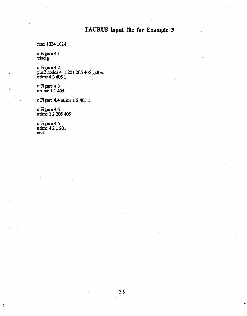
reso 1024 1024
¢ Figure 4.1triad g
¢ Figure 4.2o phs2 nodes 4 1 201 205 405 gather
nfim¢ 4 2 405 1
c Figure 4.3' nrfime 1 1405
c Figure4.4 ntim¢ 1 2 405 1
c Figure 4.5ntime 1 2 205 405
c Figure 4.6ntimc 4 2 1 201end
J
39

Chapter 5Square Plate Impacted by a Rod
FILE: D3SAMP4
5.1 SUMMARY
DYNA3D example 4 simulates a square plate impacted by a solid rod.The rod impacts and deforms the plate at the center. The plate geometryis such that the rod rebounds after impact. Key features of DYNA3D used
in thi_ example are four node shell elements, symmetry boundaryconditions, a rigid material, and a "sliding with voids" slide surfacedefinition. This model simulates a realistic response to such an impact.
5.2 MODEL DESCRIPTION
Example 4 simulates a solid rod, 4 centimeters in diameter by 25centimeters long, impacting a 62 centimeter by 62 centimeter square platein the center. The plate is supported near the edges by a plate frame thatelevates the main plate 5 centimeters from the reference ground. Themain plate is 0.79 centimeter thick and the plate frame 0.5 centimeterthick. Both parts are modeled using four-node Belytsehko-Tsay shellelements. Figure 5.1 shows the finite element mesh of the model. Table5.1 lists the material properties of the rod, main plate and plate framerespectively.
The impacting rod is given a rigid material model with eight nodebrick elements and an initial velocity of 1.Sxl0-3cm/_ts (18 m/s) into the
center of the main plate which is initially at rest. The elastic modulusspecified for the rigid material is used only for slide surface calculations.Quater symmetry boundary conditions were used on the rod.
The main plate is modeled using quarter symmetry boundaryconditions. Quadrilateral shell elements are used with an elastic/plasticmaterial model. Both the rod and main plate are given symmetric
40

boundary conditions on the x-z and y-z surfaces to utilize the symmetries
of the problem and hence reduce the number of elements by a factor offour.
A sliding with voids (type 3) slide surface is defined between the rod
and the center of the main plate as previously mentioned. This allows the
' rod to impart loads and deformations onto the plate without node
penetration.
The nodes of the innermost 4 square centimeters of the quarter
model of the plate are slaved to the bottom end of the rod which acts as
the master surface for the slide surface definition. By limiting the slave
region as mentioned, the computation time can be greatly reduced. The
vertical support plates are attached 25 centimeters out from the center of
the target plate. The nodes of thesupport plates are merged with the
nodes of the main plate, thus simulating a welded union between the mainplate and support plates.
Figure 5.2 shows the time sequence of the rod impacting the plate.The sequence lasts for 104_s. Note that the rod begins rebounding from
the plate, reversing its velocity near t = 3 x 10³_s. This event is more
clearly seen in the time history velocity plot of Figure 5.3. Node 1 (line A)
corresponds to the front left node of the main plate, node 4970 (line B)corresponds to the lower center node of the rod. One can see that in the
early and later stages of the impact the plate oscillates relative to the rod.
Figure 5.4 shows the corresponding z-displacement of the rod and
plate. The maximum deflection occurs at 3 x 10³_s after which both the
- plate and rod rebound back. At t = 4.5 x 10³_s the plate oscillates about
its final deflection of approximately 2.5 centimeters and the rod rebounds
, at a velocity of 7.0 m/s in the positive z-direction. The initial and final
kinetic energies of the rod are 0.98 kJ and 0.15 k.I, respectively. Thus, the
rod lost approximately 85% of its energy to the plastic deformation and
motion of the target plate.
41

Figure 5.5 shows the gap between the rod and the plate as a function
of time. Noto the positive finite gap of 0.1 centimeter during the simulated
contact. This is due to the measured displacements being on the rodcenterline, and the target plate cupping below the centerline of the rod.
Contact is maintained between the outer edge of the rod and the plate until
separation occurs (see Figure 5.2). This "cupping" phenomenon is
frequently observed experimentally and is accurately predicted byDYNA3D.
Figure 5.6 shows the contours of z-displacement of the main plate at
t = 1 x 10⁴ms. Note that even though the simulation is terminated at t = 1
x 104ms the plate is still responding dynamically i.e., it has not yet reached
static equilibrium. Figure 5.7 shows contours of effective plastic strain in
the main plate at t = 1 x 10⁴tns. The majority of the plastic strain occurs in
the vicinity of the impact, with a small zone along the 45 ° diagonal of the
plate due to strain wave focusing effects. Figure 5.8 shows contours of
effective stress in the target plate. Many of the contours represent the
effects of transient strain waves in the plate at this time.
Overall, this model is a good example of the robust dynamic impact
capabilities of DYNA3D.
42

RodMaterial Model 2 0
Density (g/cm3) 1.9218x101
Elastic Modulus (g/gs 2 cm) 2.1Poisson's Ratio 0.0
Main plat_Material Model 3
Density (g/cre3) 7.85
Elastic Modulus (g/gs 2 cm) 2.1
Tangent Modulus (gigs 2 cm) 1.24x 10⁻²
Yield Strength (gigs 2 em) 4.0x10⁻³
Hardening Parameter 1.0Poisson's Ratio 3.0x10" 1
Plate frameMaterial Model 3
Density (g/cm3) 7.85
Elastic Modulus (gigs2 cm) 2.1
Tangent Modulus (g/tas2 cm) 1.24x 10⁻²
Yield Strength (g/_ts2 cm) 2.15x 10- 3
Hardening Parameter 1.0Poisson's Ratio 3.0xi0-1
Table 5.1 Material Properties of Model.
43

Plate Impact by rod (cm,gm,mlcro#e_)ilme • B.
Plate Impact by rod (cm,gm,m|crosec)tlme • B.
"-'X
Figure 5.1 Finite element mesh.
44

Plate Impact, b_ roll (cm,gm,mlcrosec)time • B.
Plate Impact b_ ro_ (cm,gm,mlcrosec)time • 1.BBBBBe+B3
Figure 5.2 Time sequence of deformation.
45

Plate Impact b_ rod (cm,gm,m|crosec)tim_.. 3.00000_+0_
Plate Impact b_ rod (cm,gm,mtcrosectime • 5.00000e.03
Figure 5.2 (continued)
46

Plate lmplact by rod (cml, gm,m|crosec)time • 6.75000e+03
Figure 5.2 (continued)
4?

48

Plate impact by rod (cm,gm,microsec) INGDY4.dat
time = 1.00000e+04 contour values
contours of z-displacement A--2 35e+00B--2 03e+00
min--2.611e+00 in element 1 C--i 70e+00
max- 4.976e-01 in el_ment 489 Dm-I 38e+00
E--1 06e+00
' F--7 33e-01
i', :. ' ,' i ',i I'.. .I G--4 10e-01
._.L._....-_..1:il_._.'. :: _ :
" .... : ........ = z' ......... _{" ............ '
.._..
disp. scale factor- l.O00e+O0 (default)
Figure 5.6 Contours of z-displacement.

PAate |mpact b_ rod [cm,gm,m|croseC)t|me • I BB888e+E4 contour values' A, 3.85e-83
contours O( efr. p|ast|c straln B" 8.61e-_3
mln, 8 In element 3844 C, 1.34e-82' D" 1.81e-82
max, 4.588e-82 |n element 8 E: 2.29e-02F 2.77e-02G, B,24e-82H, _.72e-_2I, A.20e-02
e
Illllll,lll I
fliil_|llllll illIllllllllllll|lll|lllllllllllllllIIlJi|ll_illllllliillll]lllllllliliiilliilllll]ll ILII||||IIIII_IIIA[_LJ-+_II|EIlIIIIIIIIIIIIIIIIIIIIIIIIIII|IIIIJIiIIIII|I_ |lillIl£I
II_Zllllllllilllllllllllllllllllllllll_lllllglllllllllllJ.... '_' ..... ,_,'lll ,_r.................... _ ........ lll_llllJl.llllllllllllii i_ iii11111111111 IIIIIIIII i111111 I
iilll I_IIII_IIIIIIIlIlIIIIlIIIIIIIIIIIFjlIIIII_ I11•,TT_,,_4._,,UIt_ .............................................i_l_l,_:,_ll;: _::;;::::::,;,_IIIIIII::llIII_I:IIIIIIIIlIIL[
,+,--u"::i_ii:ii_iiiiiiill!iii!!!!!_!!_!!!ijiii!ii!!iiiiillIII11_1_IIi1_11_111111111111_111 11111111111111 ii11111 ii_1_1 I I i 1_1]! i i i i i i i i_1 1 i ill i i 11 i i i 1 I i ii [11 i i I I 1 i i I I i"'''--" ="_''-" ' ' '"III,,. _t x..., hl,,,, rl._ _,,,, ,,, ,,,,,
lll!]lll!llll_lll'llllllllllllllllllllllllllll]lllllllllllll
Figure 5.7 Contours of effective plastic strain.
Figure 5.8 Contours of effective stress.
5O

INGRID input file for Example 4
Plate impact by rod (em,m, mierosec)dn3dterm 1.0c+04plti 1.0e+03prti 1.0e+05c Def'me symmetry planes
• plane 20000-I 0.01 symm000-1 00.01 symmsi 1 sv;
" c Define main platestart1 9 51 63;1 9 51 63;-1;0425 31 04 25 315thl 114410.79si+l 114410.79si+l 11221 ls0010c Orientate plate slave surface towards impacting rod surface.c Always check shell surface normal vectors!mate 1endc Define left support platestart-1 ;1 50;12 11;25 0 24.5 5 4.5 0b 1 1 3 1 23 111000cFix translational DOF onbottomedge of suppoix platemate 2endc Define upper support platestart1 50;-1;1 2 11;0 24.5 25 5 4.5 0b 1 1 32 1 3 111000mate 2endc Definerod
velocity0 0 '1.8e-03start147 1013;I4 7 1013;I51;-2-2 0 2 2 -2 -2 0 2 2 5.005 30
" d010030d100300di 1 204 5;1 204 5;;
• sri - 1 -5;- 1 -5;;cy0000014sil 11551 lrnc Define bottom surface of rod as the master side of slide surface.cThissurfacehasfewernodesthanthesurfaceoftheplate,i.e.acmasterhasmany slaves.mate3end
511

cSettoleranceformcl'gebetweenmainplateandsupportscUsetp0.0001intcrac_velybeforethecontinuecommandbptol120.001bptoi 1 3 0.001cDefinematm'ialproperties
c Mainplatemat13shellro 7.85e2.1etan0.0124sigy0.0O4,pr 0.3beta1.0endmatc Supportplatesmat 2 3 sheUro 7,85e2.1etan 0.0124sigy 0.00215la"0.3beta1.0thick0.5cndmatcRodmat 3 20ro 19.218e2.1pr 0.0endmatend
/
52

TAURUS input file for Example 4
rcso I024 1024
c Figure 5.1sta_ I triad g ytrans 5 rx -90 g
c Figure 5.2, time 0g time 1,0e+03 g time 3.0e+03 g time 5.0e+03 g time 6.75e+03 g
time 1.0e+04 g
. c Figme5.3phs2nodes2 14970gatherntime6 2 14970
c Figure5.4ntime 3 2 1 4970
c Rgw-e55ro'time 3 4970 1
c Figtne 5 6plasl restore triad m 1 time 1.0e+04 contour 19
c Figure 5'7contour 7
c Figure 5.8_,ontottr9end
53

!
Chapter 6Box Beam Buckling
File: D3SAMP5
6.1 SUMMARY#
Example 5 is an excellent example of the non-linear capabilities of#.
DYNA3D. By using a specific combination of nodal boundary conditions,
shell elements, and a slide surface, a highly non-linear and unstable
buckling problem is modeled with realistic results. Key features of this
model include the use of a "single surface contact" slide surface and four
node shell elements with elastoplastic material behavior.
6.2 MODEL DESCRIPTION
Example 5 investigates the buckling of a slender beam. The beam,
made of 0.06 inch thick sheet metal, is 12 inches long and its cross-section
measures 1.75 by 1.75 inches. A quarter symmetric model is used in this
analysis. The upper 2 inches of the length of the beam is loaded by a
constant velocity field, which acts in a direction parallel to the beamslongitudinal axis.
Figure 6.1 shows the finite element mesh used with the specified
nodal boundary conditions. The mesh is composed of 1800 four node shell
elements using three integration points through the thickness. The
material model used is bilinear elastic/plastic with isotopic hardening andthe (model 3) material properties of steel. A summary of the material
properties is given in "fable 6.1.
Buckling is an unstable physical phenomena which complicates the
development of a realistic numeric model. Physically, buckling is sensitive
to imperfections in a structure, which must be incorporated in some way
into the numerical model to obtain meaningful results. This model uses a
carefully constructed mesh incorporating _odal displacement constraints
P
54
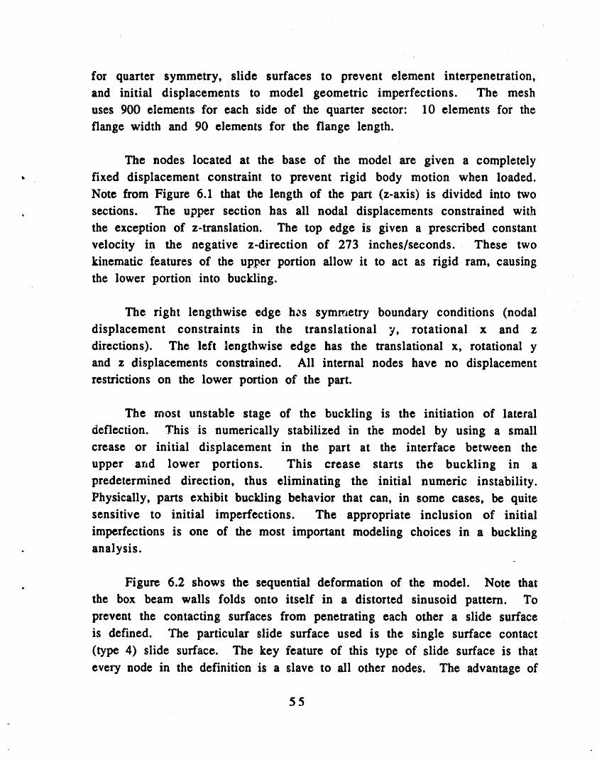
for quarter symmetry, slide surfaces to prevent element interpenetration,and initial displacements to model geometric imperfections. The meshuses 900 elements for each side of the quarter sector: 10 elements for theflange width and 90 elements for the flange length.
The nodes located at the base of the model are given a completelyfixed displacement constraint to prevent rigid body motion when loaded.Note from Figure 6.1 that the length of the part (z-axis) is divided into two
. sections. The upper section has ali nodal displacements constrained withthe exception of z-translation. The top edge is given a prescribed constantvelocity in the negative z-direction of 273 inches/seconds. These twokinematic features of the upper portion allow it to act as rigid ram, causingthe lower portion into buckling.
The right lengthwise edge h,_s sym_etry boundary conditions (nodaldisplacement constraints in the translational y, rotational x and zdirections). The left lengthwise edge has the translational x, rotational yand z displacements constrained. Ali internal nodes have no displacementrestrictions on the lower portion of the part.
The most unstable stage of the buckling is the initiation of lateraldeflection. This is numerically stabilized in the model by using a smallcrease or initial displacement in the part at the interface between theupper arid lower portions. This crease starts the buckling in apredetermined direction, thus eliminating the initial numeric instability.Physically, pans exhibit buckling behavior that can, in some cases, be quitesensitive to initial imperfections. The appropriate inclusion of initialimperfections is one of the most important modeling choices in a buckling
. analysis.
. Figure 6.2 shows the sequential deformation of the model. Note thatthe box beam walls folds onto itself in a distorted sinusoid pattern. Toprevent the contacting surfaces from penetrating each other a slide surface
is defined. The particular slide surface used is the single surface contact(type 4) slide surface. The key feature of this type of slide surface is thatevery node in the definition is a slave to all other nodes. The advantage of
55

using this type of slide surface lies in the fact that any portion of thedefined area can contact any other portion without undesirable
penetration. The disadvantage is that the computation time required forsuch a slide surface is somewhat longer than for the other slide surfaces.
Even though both the outside and inside surfaces of the model may fold
into contact, only one type 4 slide surface needs to be defined. This
surface is chosen to have normal vectors pointing toward the center or
longitudinal axis of the box beam, although outward normal vectors would
yield the same solution. ,
In the single surface contact algorithm, every segment in the
definition must check every other segment in the definition for
penetration. Thus, computation time increases greatly with the number of
segments in the definition. When using this type of slide surface, extra
time spent by the analyst in reducing the number of segments in the
definition will substantially reduce computation time and hence cost.
Many times the modeler can use engineering intuition to eliminateareas from the slide surface definition that will not contact other areas. A
few such examples can be found in this model. The upper portion used as
the ram contains 300 elements, 200 of which do not contact any otherportion. These upper 200 elements could therefore be excluded from the
slide surface definition without degrading the results. In the initial
analysis, contact of these elements in the vicinity of the buckle may have
been questionable. However, if parameter studies were to be conducted,these elements could be deleted from the slide surface definition for ali
subsequent runs resulting in a substantial decrease in run time.
Additionally, this upper portion should not contact the lower 200 or 300
elements due to the imposed displacement constraints. Here, two or three
separate slide surface definitions could be used. By dividing the slidesurface definition into three parts (upper, middle, and lower), one could
use the intuition that the upper portion might contact the middle but not
the bottom portion and the middle portion may contact both the upper and
lower portions. Computation time could be saved by using a single surface
contact definition on the middle section while the upper and lower sections
are separately slaved to the middle using a less costly type of slide surface.
56
The extent of the middle section would decrease with increased intuition of
the behavior. With the insight gained from this model one could probablylimit the slide surface definition to the middle section only.
Also of interest in this calculation is the use of four node Belytschko-Tsay shell elements with three integration points through the thickness.Three integration points is the minimum number required to capturebending with plasticity, purely elastic bending can be captured by two
-_ points through the thickness due to the linear stress distribution. Ofcourse, the more integration points used the larger the computation time,with increased accuracy in capturing a complex stress distribution throughthe thickness.
This part could have been modeled using eight node brick elements.Since brick elements have only one integration point, they would have tobe layered at least three deep to capture a stress distribution due tobending, thus substantially increasing the number of elements needed.Another consideration is the ratio of maximum to minimum lengths of thethree sides of a brick element. This aspect ratio is best kept less than fourfor reliable accuracy. Using three elements through the thickness for agiven plate thickness will thus severely reduce the in-plane dimensions ofthe element, hence requiring a very large number of small elements to beused. The formulation of the shell element does not constrain the in-planedimensions of the element regardless of the thickness, except that thethickness must be sufficiently small that shell theory is applicable. Thus,for problems where the stress gradients through the thickness are smallrelative to the in-plane stress gradients, as is the case in thin shells andmembranes, the shell element will permit fewer elements to be used when
- compared to brick elements. Also worth noting is the fact that a threenode Belytschko-Tsay shell element with three integration points through
• the thickness is only slightly higher in cpu cost than an eight node brickelement which has one integration point.
Another advantage of the shell element is the time step computed byDYNA3D. For the brick element, the time step has a linear dependence onthe minimum side length, which in the present case would be the
57

thickness. The time step computed for the shell element has a much
weaker time dependence on the thickness, thus allowing larger time stepsto be used for a given element thickness. If wave propagation through the
thickness of the structure is not of major concern, then the shell element
can be used with greater efficiency and substantial savings in cost over acomparable model with brick elements.
Overall, this problem is an excellent example of the non-linear
buckling simulation capabilities of DYNA3D_ Figure 6.3 shows the z- ,
displacement of the model after buckling. The top or ram portion of the
model has displaced almost half the original height of 12 inches with
realistic deformation. This model requires 5 cpu hours to complete on aCray XMP.
Material Model 3
Density (lbf s2/in¢) 7.1 x 10 .4
Elastic Modulus (psi) 3.0 x 10⁷
Tangent Modulus (psi) 6.0 x 10⁴Poisson's Ratio 3.0 x 10- 1
Yield Strength (psi) 3.0x10 4
Hardening Parameter 1.0
Table 6.1 Material Properties.
58

x,Y,®x,®y,®z constrained, /|
x,y,@x,@y,@z constrained, x,y,®x,®y,®z constrained,
CreaseCrease
y,®x,®z constrained ,X,®y,®z constrained
" _ ali constrained ,
Figure 6.1 Finite element mesh showing boundary conditions.
59

Beam buckle #1time - 0. Beam buckle #1 Beam buckle Q1
time - 1,20000e-03 ' time • 2.80000e-03
Beam buckle e| Beam buckle eZtlm_ • A.AOOOBe-OB time - 6.00000e-03
Figure 6.2 Time scqu¢nc¢ of mesh deformation.
6O

Beam buckle e! , Beam buckle el
time - 9.200BOe-03 time • 1.10000e-02 Beam buckle elt|me • 1.40000e-02
Beam buckle eJ
time - 1.60000e-02 Beam buckle el
time - 1.70000e-02
Figure 6.2 (continued)
61

Beam buckle #! (in,sec,lb s^2/in) INGDy5.dat i
time = 1.72000e-02 contour valuesA=-4.30e+00
contours of z-displacement B=_3.81e+00
min=-4.696e+00 in element 1660 C=-3.32e+00max=-l.277e-04 in element 910 D=-2.84e+00
E=-2.35e+00F=-l.86e+00G=-l.37e+00H=-8.83e-01I=-3.94e°-01
disp. scale factor = 1.000e+00 (default)
Figure 6.3 _ Z-disphc_m_nt after buckling.
62

INGRID input file for Example S
Beam buckle #I (in,sec,lb s^2/in)dn3dterm 1.72e-02plti 1.72e-03prti 1,0led 1201 11plane 2
" 1.375 0 0 2 0 0 0.01 symm0 1.375 0 0 2 0 0.01 symmsi 1 single;start1 11; -I; 1 74 75 76 91;0 1.375 0 0 9.7333 9.8667 10 12si 101 205 1 sb 1 1 1 2 1 1 111111b 1 142 1 5 11,0111fv 1 1 zt 2 1 5 127300-1mb 1 0 3 2 0 3 2-.02pa 1 0 3 1 -.02mate 1end
start-1;1 11;I 74 75 7691;0 0 1.375 0 9.7333 9.8667 10 12siOl10251sblll121 111111b 1 1 4 1 2 5 110111fv 1 1 4 125 127300-ImbO 1 3023 1-.02pa 0 1 3 2 -.02mate Iende use tp 0.001 intcraetively in Ingridmat 1 3 shellro 7.1e-04e 30e+06ctan 60e+03pr 0.3sigy 30e+03
. beta 1.0thick 0.06r.sri3cndmatend
63

TAURUS input file for Example S
reso I024 1024state 1c Figure 6.1triad rx -90 gc Figure 6.2restore rz-180 xtrans 1.374 razx rx -90ry 60 gtime 1.2e-03 g time 2.8e-03 g time 4.4e-03 g time 6.0e-03 gtime 9.2e-03 g time 1.1e-02 g time 1.4e-02 g time 1.6e-03 gtime 1.72e-03 gc Figure 6.3contour 19end
64

Chapter 7Space Frame Impact
File'. D3SAMP6
i
. 7,1 SUMMARY
DYNA3D example 6 uses a combination of beam, shell, and brick
elements to model an impact. The beam elements are loaded dynamically
by impact along the longitudinal axis causing the first mode of buckling tooccur. A time sequence of the deforming mesh as well as time histories of
pertinent parameters are presented to quantify the results.
7.2 MODEL DESCRIPTION
Example 6 models the impact of a rigid mass onto a thin plate
supported by a space frame. Figure 7.1 shows the quarter symmetry finiteelement mesh. The lower portion is a space frame 2 inches in diameter
and 2 inches tall, composed of beam elements. Rigidly connected to the top
of the space frame is a thin plate. A 5 lb. mass, initially 0.2 inches above
the plate, is given an initial velocity of I000 in/see towards the plate.
The space frame is constructed with three main components. The
first component is the lower ring. This uses 3 Belytschko-Schwer beam
elements for the quarter model. The end nodes of each element are given
fixed boundary conditions, hence these elements experience no loads and
are for visual _effect only. The second component is the upper ring, also
. composed of three beam elements. The end nodes of these beam elements
are merged to the local nodes of the plate, thus receiving both translational
and rotational stiffness from the plate. The third component of the spaceframe is the vertical columns connecting the lower and upper rings. Each
column has ten elements in order to capture the anticipated bending.
These columns are not perfectly straight but are slightly bowed out at
midspan. This geometric feature was incorporated as a perturbation to
help initiateand numericallystabilizethe bucklingbehavior. The beam
elementshave the cross-sectionalpropertiesof a I/4 inchsolidcylindrical
rod. The materialpropertiesof allpartsaregivenin Table7.1.
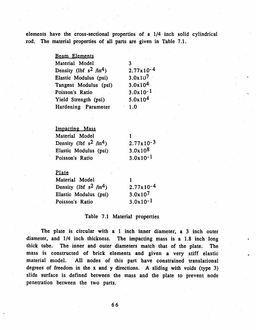
Beam Elements
MaterialModel 3
Density(Ibfs2 /in4) 2.77xi0-4Elastic Modulus (psi) 3.0x10 7Tangent Modulus (psi) 3.0x 10⁴`Poisson's Ratio 3.0x 10 _1
YieldStrength(psi) 5.0x10⁴Hardening Parameter 1.0
r
lmt_actine Mass-- w
Material Model 1
Density (lbf s2 /in4) 2.77x10- 3Elastic Modulus (psi) 3.0x10⁸Poisson's Ratio 3.0x 10" 1
PlateMaterial Model 1
Density (lbf s2 /in4) 2.77x10 -4Elastic Modulus (psi) 3.0x10⁷Poisson's Ratio 3.0x 10" 1
Table 7.1 Material properties
The plate is circular With a 1 inch inner diameter, a 3 inch outer
diameter, and 1/4 inch thickness. The impacting mass is a 1.8 inch longthick tube. The inner and outer diameters match that of the plate. Themass is Constructed of brick elements and given a very stiff elasticmaterial model. Ali nodes of this part have constrained translational
degrees of freedom in the x and y directions. A sliding with voids (type 3)slide surface is defined between the mass and theplate to prevent nodepenetration between the two parts.
66

Figure 7.2 shows a time sequence of the deforming mesh. Contact
between the mass and the plate is made at time 2.25x10 -4 sec, after which
the columns of the space frame begin to buckle. All columns buckle
outward due to the geometric perturbation.
Figure 7.3 shows a time history plot of the rigid body z-displacement
" of the mass. Maximum displacement occurs at 5.75x10 -_ sec, after which
the mass rebounds upward. Figure 7.4 shows a time his'Lory of node 54 z-
, displacement, which is located on the plate near the upper end of one of
the space frame columns. Since the deformations are symmetric and the
plate quite rigid, this can be interpreted as the vertical deflection of the
columns. Deflection begins at 2.25x10 -4 seconds and reaches a maximum
of 0.155 inches or 8% of the column length at 5.75x10 -4 seconds. The
columns regain a small portion of the deformation and oscillate about the
0.152 inch permanent vertical deflection imparted by the impact. It is
apparent from Figure 7.4 that most of the deformation is plastic.
Figure 7.5 shows the effective stress on the plate at the time of
maximum deflection. The regions of highest stress occur were the columns
attach to the plate.
u I

Z
Figure 7.1 Initial finite element mesh.
6o

Figure 7.2 Time sequence of deforming mesh.
LJ'_UP

Beam element example (in,sec,lb-s^2/in)Quarter mtime • 5.75000e-04
,,
Beam element example (|n,lec,lb-s^2/|n)Ouarter mtlme • 1.BO_SBe-03
Figure 7.2 (continued)
70

71

Y
Lx r
Figure 7.5 Effective stress contours of plate at t = 5.75 x 10.4 seconds.

INGRID input file for Example 6
Beamdement example(in,secd'b-s^2/m)Quartermodel&13d_nn 1.0e-03plli L0c-05wti9_-o4c _a_ symmetryplanes
• plam20000-I 0 0.01 symm000-1 0 0 0.01 symm
. cDefi_ slidesmfacet2tpc3si1sv;,c Beginnodedefinitionfor beamelementsc Boumnringnodesbeamcy llIlll I 0 0 cnode 1cy_ 1 15 I0c node 2cy 111111130 0c node 3cy(Xg)(gX)145 lOc node4cy 1111111600 c node 5cy_ 175 10c node 6cy 111111190 0 c node 7camies 2,4,6, and 16 are used for aligning cross-sectional propertiesofc beamelen_ntsc enkidlenodescy 000110 1.01 0 1 c node 8cyO001101.01 30 1 c node9cy000110 1.01 60 1 c node 10cy 000110 1.01 90 I c node 11
c topringnodescy_ I02 cnode 12cy _ 1 30 2 c node 13cy_ 160 2c node 14cy_ 190 2c node 15cnormalvector node for vertical elementscy(XXggg)0 0 1 cno(le 160c Beginbeamelementdefir_tionc denznts for bottomring
• 131112351114571116c eknz_ fortop ring12 131 1 1 213141 I14141511 I6c venial elementsft-orebottomto middle1851116395 1 1 16510511167 115 1 1 16
73
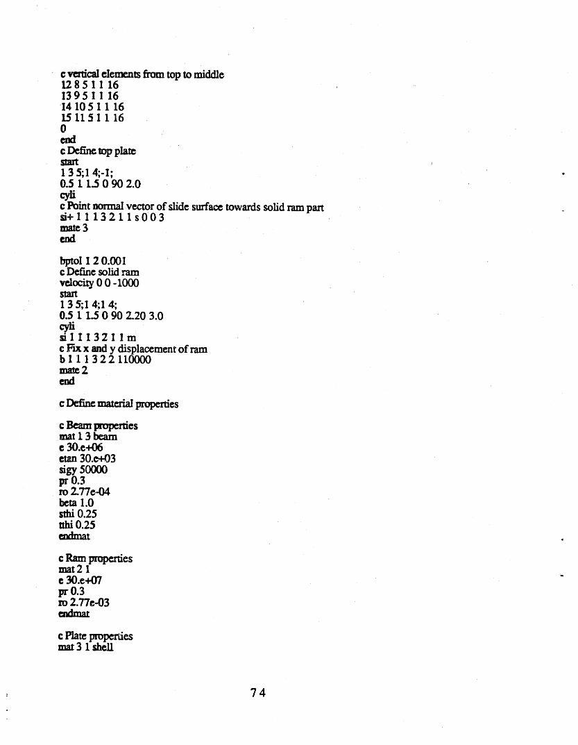
¢verticaleJcmcntsfromtoptomiddle1285 !1161395 !I1614105 11161511511 160endcDeEn¢topplate
135;I4;-I;0.51 1.50 902.0cylicPointnormalvectorofslidesurfacetowardssolidrampartsi+l11321 Is003ma_3end
bptol12 0.001cDefinesolidramvcZoc'_0 0 - 1000start13 5;I4;14;0.51 1.50 90Z20 3.0
sillI32Ilme Vuxx andy displacementof ramb 11 1 322 110000nuee2end
c DefmematcriaIproperties
e Beamt,mperdesmat13 beamc 30.c+06etan30.c-t03sigy5OOOOpr0.3ro 2.77e-04beta1.0stiff0.25nhi0.25endmat
cRam pmpcrticsmat21c 30.e+07pr0.3m 2.77c-03endmat
c Platepmpcrdcsmat3 1shell
74

e30.e+06ro2.77e-O_tpr0.3thick0.125endmat
end
75

TAURUS input file for Example 6
reso10241024c Figure7.1statetrx-90ry15triadgrestore razx myz triad rx -90 ry 15c Figure 7.2state 1 gtime 2.0e,04gtime 5.75e-04 gtime 1.0e-03 gc Figure 7.3phs2 marls 12 nodes 1 54 gatherretiree 3 12c Figure 7.4ntime3 154cFigure7.5phsltime5.75e-04rims1 3rx90 contour9end
76
E

Chapter 8Thin Beam Subjected to an Impact
File: D3SAMP7
. 8.1 SUMMARY
. DYNA3D example 7 is a simple model of a thin beam subjected to a
transverse impact load. The key features of this model are the use of four
node Belytschko-Tsay shell elements and the modeling of dynamic bending
response. Stresses and strains through the thickness of the beam, as well
as kinematic responses, are plottedand examined as a function of time.
The dynamic responses compare favorably to approximate analyticalresults.
8.2 MODEL DESCRIPTION
Example 7 models a thin rectangular beam 0.6 inches wide by 10
inches long with a thickness of 0.125 inches. Symmetry is used about the
plane in the center of the span thus reducing the number of elements byone half. Figure 8.1 shows the finite element mesh. The end boundary
condition is fixed with the displacements on the x-z surfaces constrained in
the y-direction.
Ten four node shell elements are used, with five evenly spaced
integration points through the thickness (trapezoidal integration). Using
the trapezoidal integration option with three or more points in odd. increments allows the surface and mid'plane stresses and strains to be
captured exactly, as opposed to using Gauss quadrature which requiresthese stresses and strains to be extrapolated or interpolated. The shell
elements are given the elastic/perfectly plastic material properties of6061-T6 aluminum using material model 3 in DYNA3D. These propertiesare listed in Table 8.1.
77

Material Model 3
Density (lbf s2/in 4) 2.61x10 "4
Elastic Modulus (psi) 1.04x10⁷
Tangent Modulus (psi) 0.0Poisson's Ratio 3.3x10" 1
Yield Strength (psi) 4.14x 10⁴
Hardening Parameter 1.0
Table 8.1 Material Properties.
The middle 2 inches of the ten inch span are give_ an initial velocity
of 5,000 in/see in the negative z-direction. The response is simulated for
1.75 milliseconds. Figure 8.2 shows a time sequence of the deforming
mesh with it,= symmetric reflection. Figure 8.3 shows the kinematic
responses of node 19, which is at the center of the span. The simulated
impact produces a maximum deflection of 0.78 inches at the center. Thisdeflection, more than four times the shell thickness, is sufficient to make
large deformation effects important in this problem.
The low frequency transverse structural vibration resulting from the
impact can be seen most clearly in the displacement response. Note that
the center of the span is oscillating in time. The period of oscillation is
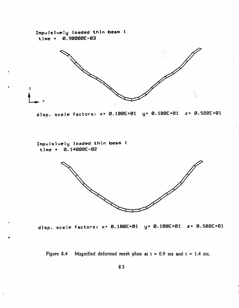
approximately 0.6 milliseconds. Figure 8.4 shows the deformed mesh at0.9 milliseconds and 1.4 milliseconds with the z-displacements amplified
by a factor of 5. The deformed mesh at 0.9 milliseconds has three troughsand four crests over the span. This shape occurs again at 1.4 milliseconds
which is in the second cycle of structural vibration. These transverse
waves propagate from the center of the span to the fixed ends where they a
are reflected back towards the center for another cycle.
The shapes in Figure 8.4 are characteristic of the third mode ofvibration. Elastic txansverse vibration theory for a fixed end beam with
similar stiffness and mass properties predicts a third mode natural period
of 0.7 milliseconds. Even though the model experiences plastic strains, theelastic theory can be used for an approximate comparison. The first and
second modes are not distinguishable in the given time interval. Higher
78

modes can be seen in the velocity and acceleration responses but they are
indistinguishable in the deformed geometry plots, because their
amplitudes are relatively smaller.
Figures 8.5-8.7 show the effective stress and effective plastic strain
of the center element. Figure 8.5 corresponds to the bottom surface of the
element. Figure 8.6 corresponds to the internal mid-plane surface, and
• Figure 8.7 to the top surface. The bending stresses add to the membranestresses at the bottom surface and subtract from the membrane stresses at
top surface, thus the bottom fibers suffer the most plastic strain. The
membrane stresses appear to be significantly larger than the compressivei
bending stresses on the top surface.
Stresses and strains through the thickness of a shell element are
selected in post-processor TAURUS by using the Shell inner, Shell
middle, and Shell outer commands prior to the stress or strain display
command. For this model, three trapezoidal rule integration points
through the thickness would have been sufficient to capture the three
stress planes discussed.
Impulsively loaded "Lhtn beam (t; I me " 0. 00000E+00
elemen+, numbers
[ I I I I I. 4 I 5_ I I I 8 1 Fixed. Plane
y
Figure 8.1 Finite element mesh.
79

uII ,
Impulsively loaded rhlh beam (t Ime I 0.81B_OIBE+00 '
i l ii i[ ] i LI
Z
Impu Is Ively loaded, 'thln beam ('tIme • 0. IBIBIBIBE-_I3
i
iiiii I i _ ilip L III _ III
L
r
Impulsively loaded thln beam (, t i me - B, 2000BE-B3
T
• T I
Figure 8.2 Mesh deformation sequence.
80
f
J

Impuls|vel 9 loaded th|n beam ($ Ime - B. 300{BBE-B3
. Z
, Impu Is IvelLI loaded thin beam (t|me - 0.TBO{BOE-B3
Impu is Ively loaded $h|n beam (t !me - B. 9000BE-B3
Figure 8.2 (continued)
81

4.OR
-I.M
"'TI"'T!'"T!
|'"I /
°?,DI_,4: _
•,,Inlu • 4.'J_Ol[_lJO aolJe I'D
laipulolv_ly Ioodtcl thlr_ bee- |
Figure. $.3 Kinematic r_sponscs of nod_ 19°
82=
_"'1|_ nrVll,' ' llliP+ r_ 'PA '" q"'
Impuls|ve_'y loaded thin beam (t I me - B. 90000E-03
d|sp. scale t'actors: x- 0.100E+01 El" 0.100E+01 z" 0,500E+01
Impulsively loaded thln beam (t | me - 0. 14000E-02
d|sp. scale Cactors: x- 0.100E+01 _- 0.100E+01 z- 0.500E+01
Figure 8.4 Magnified deformed mesh plots at t = 0.9 ms and t = 1.4 ms.
83

|au_ulallvelLj ollded thin i_em ¢
4.__ " " " ' ......... -" " "+.... ' "' TM
III_l.'l'iC
I
_ _._,_m
y.gllE,l_
I||I|H||III_MHV|H_|IHItn_ • l.i_ OIImnontl gm,,lu • 1.4141£_ +++lm+
lNulelwl U lold_ thln I=eeR ¢
Figure 8.5 Effective stress and effective plastic strain of clement 9 bottomsurface.
,
In
r, $4
2

Impulsl_l V Io_larct thin teem (" • • • r • • • • • • • ,v • • , • • s'
4. all(*O, _I
I,v'.J[.e, Ik
II.Ml[*.lk t
II.llltl_ II.mE*l_
Z.rll_ / t- JL.
l
I._*ti
"/ ? ," _ ?li ttlttll tl.WMt_tt _ Itt_ .: ,_ ,__ ,_ _ ,.....• P ,. .:..'- ...: ._ ._ ._ ._ ,_
mlnlu o l.l_lll lllmB_ttl I
_:I_ * II,41,lI£*I15 t |me
|mp, lalvei H Ioaidm.d thin iea.- |
Jll|lli|ll|l_li_||_lil
Figure 8.6 Effective stress and effective plastic strain of element 9 mid-plane.
85

lq)u3_lwly Iooded thin bean (i i v • • • • • • i • • • • •
t.,,,=..,. " " " /..r
t,,'m:-,m /
|•1_,,tli
£ I 0,1R,,_
_ l._-a ,_s-om I° I_,,tm
U I. llr,.41_
ol | • lm',.41aa
-- I.I-41Qa.
I.I-02
,..- ?.II:.413
_. S. IK,.OIb
40_,_
I,IMI. _
Ihlll.4m
I .aK-II3
Ittllllllll-I_l_tl_lllminim • I,I¢11 elmtl •II_i • I. ll41 _Llle
Figure 8.7 Effective stress and effective plastic strain of element 9 topsurface•
' 86

INGRID input file for Example 7
Impulsivelyloadedthinbeam(in,scc,lbscc^2/in)dn3d /
term2.0c-03prti1.0 ' ,,'/
plti 1.0c-OS,{_', il ,,cDefineindexspaceandcoordinatesforouterportionstart4 11;I2;-1;
t 1.5 5.0 0._0,6 0.c Set lengthwise edge boundary conditionsb I 1 12 1 1010101b 1 2 1 2 2 1 000101c Set fixed end boundary conditionb2 1 122 1 111111mate 1end
c Define index space and correspondingcoordinatesfor center portionc that is giveninitial velocitystart1 4;1 2;-1;0 1.5 0.6 0c Set symmetryboundary conditions on centerb 1 1 1 12 1 110111c Set symmetryboundary conditions on centerb 1 1 1 12 1 110111c Set lengthwise edge boundary conditionsb 1 1 12 1 1010101b 1 2 1 2 2 1 000101velocity 0. 0. -5000.nmte1end
c Use tp 0.001 interactively in INGRID
c Definematerialpropertiesmat 1 3 shellc 6061-T6AL (ro .261e-03 t• 10.4e+03pr 0.33
'_ sigy 41.4e+03etan0.0beta1.0thick0.125tsti5cndmatend
87

TAURUS input file for Example 7
reso 1024 1024Figure 8.1time0 elplt
c Figure 8.2rayzrx -90 g time .le-03 grime .2e-03 g time .3e-03 g time .5e-03 gtime .7e-03 g time 0.9e-03 g time 1.6e-03 g
c Figure 8.3phs2 nodes 1 19 gather vntime 3 1 19ntime 6 1 19
c Figure 8.4phs1 dsfs 1 1 5 time .9e-03 g time 1.4e-03 g
e Figure 8.5phs2 elements 19 gathershell inner etime 9 1 9 etime 7 19
c Figure 8.6shell middle etime 9 19 etime 7 19
e Figure 8.7shell outeretime 9 1 9 etime 7 19end
88

Chapter 9,Impact on a Cylindrical Shell
File: D3SAMP8
9.1 SUMMARYA
t DYNA3D example 8 simulates an impact on a section of a cylindricalshell. The key feature of this example is the large plastic deformation of
four node Beiytschko-Tsay shell elements. Contour plots of stress, strain,
and displacements as well as time histories of nodal displacement, velocity,
and acceleration are presented. The resulting displaced shape as well as
through-thickness stresses and strains are representative of a physicalimpact of such a structure.
9.2 MODEL DESCRIPTION
Example 8 models a section of a circular cylindrical shell with a
radius of 2.938 inches, length of 12.56 inches, and thickness of 0.125
inches, subjected to an impact load that causes large deformation in the
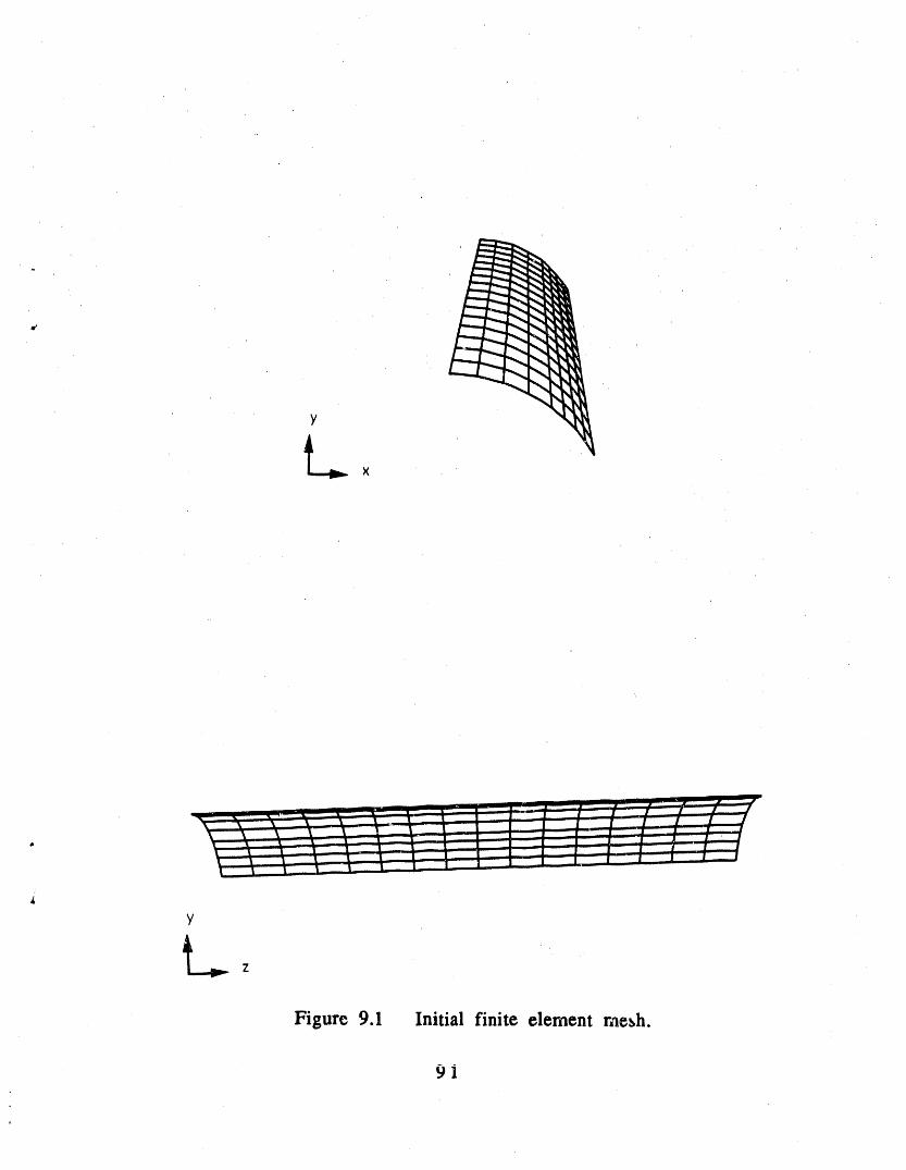
radial direction. Figure 9.1 shows the finite element mesh used in this
model. Symmetry is used about the y-z plane by constraining the nodal x-displacements as well as y and z rotations. The ends of the cylinder have
the x and y displacements constrained while the bottom edge has alidisplacements and rotations constrained.
The elements used in the model are four node Belytsehko-Tsay shellelements with 5 gauss integration points through the thickness and the
material properties of an elastic/perfectly plastic 6061-T6 aluminum.
Each element has a uniform thickness of 0.125 in. A summary of thematerial properties can be seen in Table 9.1.
An initial velocity of 5650 in/see in the negative y-direction is givento 65 interior nodes. The resulting deformation can be seen in the time
89

sequence of Figure 9.2. The deformed mesh is shown with its symmetricreflection for clarity.
Material Model 3
Density (lbf s2 /in4) 2.50x10 .4
Elastic Modulus (psi) 1.05x 10⁷
Hardening Modulus (psi) 0.0Poisson's Ratios 3.3x 10- 1
Yield Strength (psi) 4.40x10⁴
Hardening Parameter 1.0
Table 9.1 Material properties.
Figure 9.3 shows the kinematic response time histories of node 8,
which is centrally located on the top of the shell. The maximum deflectionof 1.27 inches occurs at 0.4,25 milliseconds in the 1.0 milliseconds
simulation. Ali plots show structural vibration as a result of the impact.
The lowest mode appears to have a period of approximately 0.7milliseconds as seen in the displacement response. Higher modes can be
found in the velocity time history.
Figure 9.4 shows contours of y-displacement at 1.0 milliseconds. The
deformed shape is representative of a real impact on such a structure.
Figures 9.5-9.7 show contours of effective stress and effective plastic
strain of the inner, middle, and outer integration points through thethickness, respectively.
Note that the maximum effective plastic strain of 42.1% occurs on
the irner surface of element 78, and 25.2% on the outer surface of element
82, while the midpoint maximum effective plastic strain is less than 13.4%.
This strain distribution is the result of both membrane and bending ,stresses. These high strains occur near the lengthwise crease in the shell.
This model is a good example of the use of four node shell elements
combined with an elastic/plastic material model to analyze a thin-walledstructure under impact loads.
90
Y
Lx
Figure 9.1 Initial finite element me_h.
9i

C_11_drlcal shell (ln,sec,ib s^2/in)tlme • B.
C_iindrlczl shell (In,sec,ih s^2/in)t I me • I. 88_0e'04
C_ll_drlcal shell (in,sec,l_ s^2/lh)t|me • 3.88_0_-04
_,,,,,, , ,_, , /.// /__
Figure 9.2 Time sequence of mesh deformations.
92

Cclllndr|cal shell (In,see, Ib s^_/in)t i me • 5. 00000e=04
. Z-ililil l I... s ,
Cyllndr|cel shell (ln,sec,lb slA2/In)tlme • 7,00000e-04
C_lindrlcal shell (in,see,lh s^2/in)tlme • 1,00000e-03
• +
EJ' i ......
'i-i][,_"i ] I I i I !...I-_
Figure 9.2 (continued)
93
,, lip, ,

Cylindrical mhell (In,_ec,lb
Figure 9.3 Kinematic response time hist,_ries of center node.
94

4'
CBI Indr foal shell In,sec, Ibtlme - 0.10000E-02 contour valuesR--l, 03E+00.ontours o_ y-dlmplacemenl _;,-9.06E-0111n--B.i1BE+01 _n element 21 C--7.BBE-01mx= 0.5t8E-01 In element IIB D=-6.60E-01
E--5. BBE-01F--4.15E-01G--2.9BE-BlH--1.70E-01I "-4.7BE-02
d|mp. scale _motor - 0.100[+01 (default),J
, Figure 9.4 Contours of y-displacement,

Cyl|nUrlcsl shell (In.see, lhtime • 9.1eeseC-e2 contour values
A- 6.esc.e_:ontours o¢ etf. stress (v-m) B. 1.11[,64s|e. B,D45r¢_4 |n element 25 C- 1.5_I_*B4• i-. 9.44Br¢05 in element 182 D- t.gsr+B4
r. 2. aTr,e4r, 2.?gC.i_G- 3.22[_@4H- 3.64[¢64! • 4. B&[*B'I
dlsp. scale Tsc_or • 0.IBeX*BI (deSau_t)
C_llnelrlcal shell (In,sac, lbt|me • B.|aBB_;'-B2 ©antovr _alues
R. 3.54[-E2contours o_ e¢¢. plastic strain 5, ?.91[-82mln- B.BBg[*BB _n element 127 C- 1.23['01max. B.42J[¢BB In e|lrment 78 D, t.87E:-B1
2.5.'1[-B1G, 2.98[-B1H, 3.42[-B1!. 3.B6[-Et
disp. scale factor - 8.|BB[¢E! (deTault)
Figure 9.5 Effective stress and effective plastic strain contours of innerintegration point.
96

CWiindPIcal shell (In,sec,,lID COntOUr valuestime • I. SiBeBr-B2 A- ?.GB[.B3
contours o; rf{. otrimm (v-m) B, 1.12[.B4.04C- I Bg*E4
E.B95[.B5 element 125 D, _.21'05[*B4[, :P 1[ ._B4r, Z. 5Tr.B4
Gi 2.9'['B'13.29[.043. G5£+64
__.__N dlsp. scale {sefor " 0.169[.61 (de_avlt)
Cglindrlcal ol'_]l (lh,see, lhtime • B.1BBBB£-B2 contour valuesA- 1.12[-82
contours of rf{. plastic strain B, _ 51[-02mln, B.BBB[.BB In element 127 C- ,:gB[-B2max, O.l)4[.OO In element 81 D, 5.29[-02[- 6.69[-02
F, 8.00[-02G, S.47[-=2H, 1.Eg[-BI;, 1.23[-B1
dlsp. scale {actor • O.lOO[.O5 (default)
Figure 9.6 Effective stress and effective plastic strain contours of middleintegration point.
97

Cuilncl:rl©ol ol'_,ll (In,nec,Ilotime • 0.1BBSG£-B2 contour _o|ueli
I:1- O. ?1[+B3contours of efr. IltrlmS (_r-m) B" |.Z?£.O4mis, O.S4_rlC.B4 In element 95 C- l.G?C.O4m41x, O.44K.B5 In element ?El D, 2.BTr.84
r, 2.47[.B4lr • 2. BTE.BIG, 3.2BI.B4H. 3. SSr'+i_l!. 4. BIr.B4
N disc. scale factor • 8.1B8[.O! (default)
CuItndrlcol ol",e_l (In,lee, lhtime • 8.|8BBB[-B2 contour +llull
_" 2.t2['m2contours Of cfC. plactic strain B" 4.74[-82ats, B.399E-B4 In element 12G C- ?._S[-O2Nx, O.ZS2[+O8 In eJlmsnt 02 D" 9.97E-B2
£" t.2S[-e!r, t. 52[-B !G, t.?OE-B!H, 2.BSE-B!I, 2.a1[-81
olimp, stole Csctor - II. IBeE.B! (default)
Figure 9.7 Effective stress and effective plastic strain contours of outerintegration point.
98

INGRID input file for Example 8
Cylindrical shell (in,sec,lb s^2fm)dn3dterm 1.0c-03plti 1.0e-05prti 1.0c Define symmetry plane
" plane I
0 1 0-1 0 0 0.0001 symm
• cDefineimlerportionofcylinderwithinitialvelocitycIndexspaceandcorrespondingcylindricalcoordinatesvelocity0.0-56500start-1;I5;214;2.93890 52.5-0.785-10.205
cylimateIend
cDefineouterportionofcylinder,notevelocitiesareresettozero.cIfthiswerenotthecaseallelementsinthispartwouldhavethecaboveinitialvelocity.velocity0 0 0start-1;15 9;12 1417;2.9389052.530 0-.785-10.205-12.56
cytic Fix alldisplacementson bottomedgeb I3 1 134 111111cFixx andy translationonendsbl 1 1 13 1 1100000b 114 134 110000
c Delete region that corresponds to the ftrst partdefinitiond112123mate 1endc use tp 0.001 intcractively in INGRID
c E_fine material propertiesc 64)51t-6 AL
' mat: 1 3 shellthick 0.125ro2.5e-04
I, • 10.5e+06etan 0.0pr 0.33sigy 44.0e+03beta1.0tsti5endmatend
99

TAURUS input file for Example 8
reso 1024 1024triadc Figure 9.1state 1 rx 15 g rx -15 ry 90 g
c Figure 9.2restoretraidrayz ry 45 g time .1e-03 g time .3e-03 g time .5e-03 g time .7e-03 gtime 1.e-03 g
c Fi_u'e 9.3phs2 nodes 1 8 gatherntime 2 1 8 nfime 5 1 8
c Figure 9.4phsl restore rayz rx25 ry25 fimel.Oe-03contour 18
c Figure 9.5shell inner contour 9 contour 7
c Figure 9.6shell middle contour 9 contour 7
c Figure 9.7sheU outer contour 9 contour 7end
100

Chapter 10Simply Supported Flat Plate
File: D3SAMP9
• 10.1 SUMMARY
i DYNA3D example 9 investigates the response of a simply supported
flat plate subjected to a rapidly applied uniform pressure load. Response
parameters such as maximum deflection, natural frequency, and maximum
stress are compared with analytical results. The DYNA3D results are in
close agreement with the analytical solutions.
10.2 MODEL DESCRIPTION
!
Example 9 models the response of a simply supported flat plate
subjected to a rapidly applied uniform pressure load. The 10 inch by 10
inch, 1/2 inch thick plate is modeled using two planes of symmetry: the x-
z plane and the y-z plane as seen in Figure 10.1. A total of 16 elements
are used in the quarter model, each having five gauss integration points
through the thickness. Material model 3 (elastic/plastic) is used with the
properties of a perfectly elastic aluminum (the yield stress is set
artificially high to prevent plasticity). A summary of the material
properties is shown in Table 10.1.
Material Model 3
Density (lbf s2 /in 4) 2.588x10 -4
Elastic Modulus (psi) 1.0x 10⁷
Hardening Modulus (psi) 0.0/, Poisson's Ratio 3.0x I 0" 1
Yield Strength (psi) 1.00x 10⁵
Hardening Parameter 1.0
Table 10.1 Material properties
101
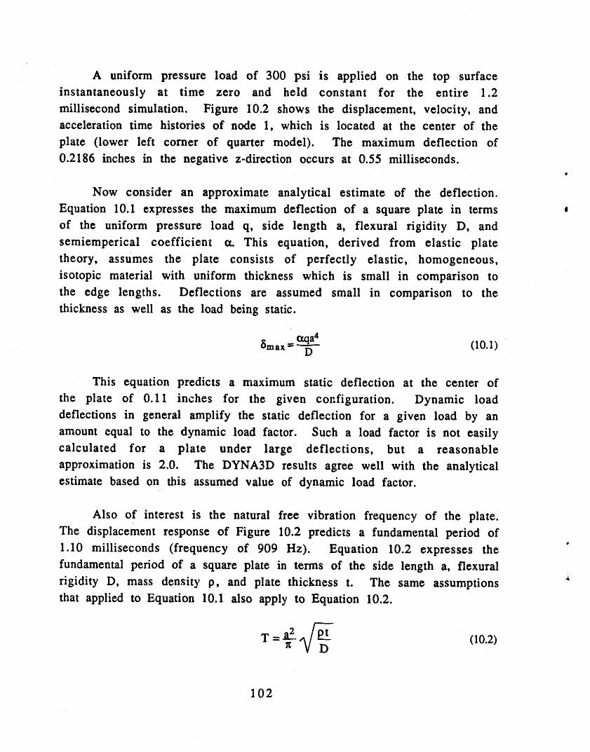
A uniform pressure load of 300 psi is applied on the top surface
instantaneously at time zero and held constant for the entire 1.2
millisecond simulation. Figure 10.2 shows the displacement, velocity, andacceleration time histories of node 1, which is located at the center of the
plate (lower left corner of quarter model). The maximum deflection of
0.2186 inches in the negative z-direction occurs at 0.55 milliseconds.t
Now consider an approximate analytical estimate of the deflection.
Equation 10.1 expresses the maximum deflection of a square plate in terms 0
of the uniform pressure load q, side length a, flexural rigidity D, and
semiemperical coefficient ¢_. This equation, derived from elastic plate
theory, assumes the plate consists of perfectly elastic, homogeneous,
isotopic material with uniform thickness which is small in comparison to
the edge lengths. Deflections are assumed small in comparison to thethickness as well as the load being static.
o_a46max = "-'_'-- (10.1)
This equation predicts a maximum static deflection at the center of
the plate of 0.11 inches for the given configuration. Dynamic load
deflections in general amplify the static deflection for a given load by an
amount equal to the dynamic load factor. Such a load factor is not easilycalculated for a plate under large deflections, but a reasonable
approximation is 2.0. The DYNA3D results agree well with the analytical
estimate based on this assumed value of dynamic load factor.
Also of interest is the natural free vibration frequency of the plate.
The displacement response of Figure 10.2 predicts a fundamental period oft_
1.10 milliseconds (frequency of 909 Hz). Equation 10.2 expresses the
fundamental period of a square plate in terms of the side length a, flexural
rigidity D, mass density p, and plate thickness t. The same assumptionsthat applied to Equation 10.1 also apply to Equation 10.2.
T = a_. _/_ (10.2)V D
102

This equation predicts a fundamental period of 1.07 milliseconds
(frequency of 935 Hz), which is in excellent agreement with the DYNA3Dresults.
Figure 10.3 shows a time history plot of the stress Oxx in element 1,
, which is located at the center of the plate. This plot corresl_onds to the
bottom or tension surface of the plate. The response of the stress a yy is, identical due to symmetry. The peak stress occurs 0.03 milliseconds prior
to the maximum deflection with a value of 67.7 ksi. Using a maximum
deflection of 0.22 inches in Equation 10.1 and solving for the load q gives619 psi. Equation 10.3 expresses the maximum stress axx, max in the
plate in terms of the load q, side length a, thickness t, and semiempirical
coefficient 13. This equation is also based on elastic theory. Using a load of
619 psi in Equation 10.3 yields a maximum stress of 71.2 ksi, which agreeswell with the numerical analysis.
%x, max = -_qa2 (10.3)t 2
Figure 10.4 shows a contour plot of the z-displacement at t = 0.55 ms.
The mesh shown has the x-z and y-z planes reflected symmetrically for
clarity. The displaced shape is in good agreement with analytical contourplots. Figure 10.5 shows the axx contour plots for the upper, middle, and
lower quadrature points through the thickness at time equal 0.55 ms.
Slmply support, cd plate (ln,sec, lb s^Z/ln)_.lme = 8.
----- i --.
q lm ,nii -- iiimll
,, , ,, _,_.
II
i ii ii
/ /_.......... i&Figure 10.1 Initial finite element mesh of plate.
103

104

105
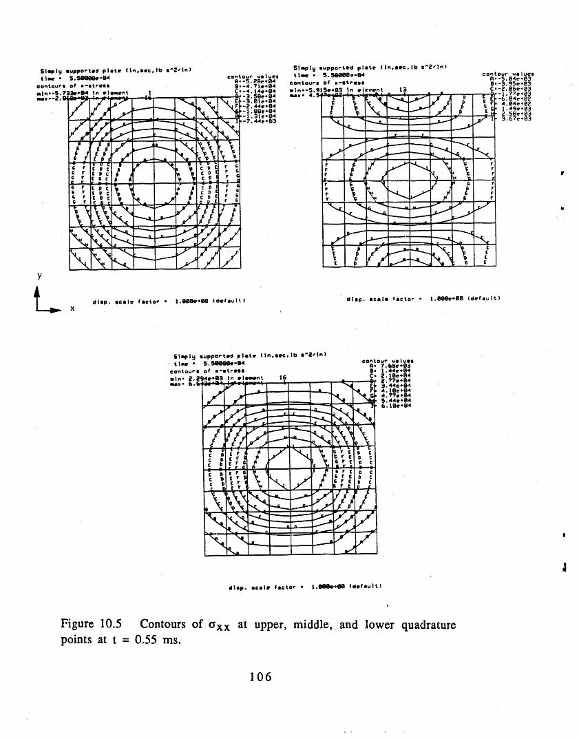
Simply supported plate (In,soc,Ilo s_Z/In) Slipl W supported plote (in,soc,lh s*2/In)time • S.581DEee-84 contour values time *' 5.Seeoe_-B4 contourA,.S.O4e,e3values
I_.-5._SL**B4 contours of w-stress B,-3.95e*B3i:ontours of li-Stress B,-4.71e.B4m|n,-5.?33e.B4 In ellment ! C--4.14eM_4 mln,-).?l)e+i_3 in eloquent |3 C.-z.e6e_;}3
¢ O [ r Vl _-c_l r _ r
k_l.'_.'-'--"" ,f .7- _ _
y
dlsp. so,le l_cl.or * II.II08e.IIIil(deCsult) dlsp.
lille (scto_ (clef muir)
X
Slmpl W supported piero (In,soc,lh s'Z/In)' tlae • 5.Si_li_e-B4 contour '.*sluesii" 7.6Be.03COntourS Of li-ItrIII B" |.44e.I_1
sin. 2.294e+i_ In ellmen_ |6 C, "_:|i_e.i_4??e.B4
_,, 6. _ " ....IL • _ 4. li_e.04
J _ ..77e.04- 5.44e.O4
],.,,r [ D __lr_..
N ---_
1
41ltp. scale factor • l,gl_he*_l_ (default)
Figure 10.5 Contours of 6xx at upper, middle, and lower quadraturepoints at t - 0.55 ms.
106

INGRID input file for Example 9
simply supported plate (in,sec,lb s^2/in)dn3dterm 1.2e-03plti 2.0e-05prti 2.0e-041cd 1 2 0 1.0 1.0 1.0
' cDefine symmeuy planesplane 21.0 0.0 0.0 -1 0 0.001 symm0.0 1.0 0.0-1 0 00 0.001 symmc Define index space and correspondingcoordinatesstart1 5;1 5;-1;0 5.0 0 5.0 0.0c Fix y displacement on outside edgesb2 1 1 22 1 001000b 1 2 122 1 001000c Define applied pressure regionpr 1 1 1 22 1 1 300.0 0 0-1cSpecify element printout blocksepb 0.0 0.0 0.0 0.625 0,625 O;mate Iende Specify hourglassing parametersqh 0.05ql 1.2cDefine materialmat 1 3 shellc aluminumro .2588e-03e 10.0e+06pr 0.3sigy 100.0e+03etan 0.0beta 1.0thick 0.5tsti 5endmatend
107

TAURUS input file for Example 9
reso10241024cFigureI0.IstateIrx-75g
cFigure10.2phs2 nodes 1 I elemenc_ 1 1 gather ntime 3 1 I ntime 6 1 1 ntime 9 1 1
c Figure 10.3 shell inner
crime 1 1 1
cFigur_:10.4phsl restore razx r_yztime 0.55e 03 t'_ntour 19
I
cFigure10.5shelloutercontourIshellmiddlecontourIshellinnercontour1end
lt
108
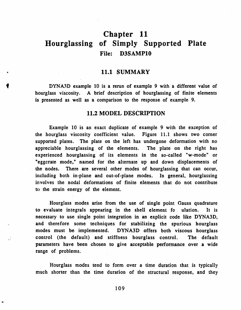
Chapter 11Hourglassing of Simply Supported Plate
File: D3SAMP10
• 11.1 SUMMARY
DYNA3D example 10 is a rerun of example 9 with a different value of
hourglass viscosity. A brief description of hourglassing of finite elements
is presented as well as a comparison to the response of example 9.
11.2 MODEL DESCRIPTION
Example I0 is an exact duplicate of example 9 with the exception of
the hourglass viscosity coefficient value. Figure 11.1 shows two corner
supported plates. The plate on the left has undergone deformation with noappreciable hourglassing of the elements. The plate on the right has
experienced hourglassing of its elements in the so-called "w-mode" or
"eggcrate mode," named for the alternate up and down displacements of
the nodes. There are several other modes of hourglassing that can occur,
including both in-plane and out-of-plane modes. In general, hourglassinginvolves the nodal deformations of finite elements that do not contribute
to the strain energy of the element.
Hourglass modes arise from the use of single point Gauss quadrature
to evaluate integrals appearing in the shell element fo _ulation. It is
necessary to use single point integration in an explicit code like DYNA3D,
. and therefore some techniques for stabilizing the spurious hourglass
modes must be implemented. DYNA3D offers both viscous hourglass.! control (the default) and stiffness hourglass control. The default
parameters have been chosen to give acceptable performance over a wide
range of problems.
Hourglass modes tend to form over a time duration that is typically
much shorter than the time duration of the structural response, and they
109

are often observed to be oscillatory. Hourglass modes that are a stable
kinematiccomponent of the globaldeformationmodes occur over a much
largertime frame and must be admissible. Therefore,DYNA3D resists
undesirablehourglassingwith viscous damping capable of stopping the
formationof anomalous modes but havinga negligibleaffecton the stable
global modes. Since the hourglassmodes are orthogonal to the real
deformations, work done by hourglass resistance is neglected in the energy
equation. This can lead to a slight loss of energy, however, hourglassviscosityshouldalways be used.[7] t
The default value for the hourglasscoefficient is 0.10. The
recommended range is 0.05 to 0.15. These values apply equallyto the
shellsand eight-nodebrickelement. The values used in examples 9 and
I0 are 0.05 and 0.005respectively.The qh command in the pre-processor
INGRID is used to specifythisvaluewhen differentfrom the default.
Figure 11.2 shows the kinematic responses of the center node of the
plate. As a result of reducing ',he hourglass coefficient an order of
magnitude, the displacement of the center node has increased slightly inamplitude. The maximum deflection of-0.2213 inches occurs at 0.55
milliseconds, compared to the maximum deflection of D3SAMP9, -0.2186
inches, also occurring at 0.55 milliseconds. This node then rebounds,
reaching a maximum positive deflection of 0.0036 inches. The response ofexample 9 rebounded to 0.0000 inches. Both of the maximum rebound
deflections occur at 1.1 milliseconds. The difference is small (4%), and it is
not apparent which is more accurate.
The velocityresponseof the centernode shows a similaramplitude
increase. Example I0 with the lower hourglasscoefficientshows a 4%
largeramplitudethen example 9. Evidence of high frequencyoscillationis
apparent on the example 10 velocity plot which is not the case with
example 9, although this oscillation is not necessarily a direct result ofhourglassing.
An 8% increasein accelerationamplitudecan be found in example I0
when compared to example 9. Figure 11.3 show the x-directionstresstime
110

history of the center element. A 2% increase in peak stress can be found inexample 10 response over example 9.
Thus, although small, the damping effect of the hourglass coefficientcan be seen, especially in the velocity and acceleration responses. Notefrom the z-displacement and x-stress contour plots (Figures 11.4 and 11.5)that no hourglass modes are apparent. This example problemdemonstrates the more subtle aspects of hourglass control, i.e., the effect of
| hourglass control parameters on the various response parameters asopposed to outright element hourglas_dg. As mentioned above, thehourglass control is not intended to affect normal modes of deformation,
but from this example it is seen that it can. The difference in responsesbetween example 9 and example 10 are quite small. Any adjustment ofthis parameter is best left to the experienced user.
111

Without hourglassing
With hourglassing
Figure I1.1 Example meshes illustrating the effect of hourglassing.
, 112
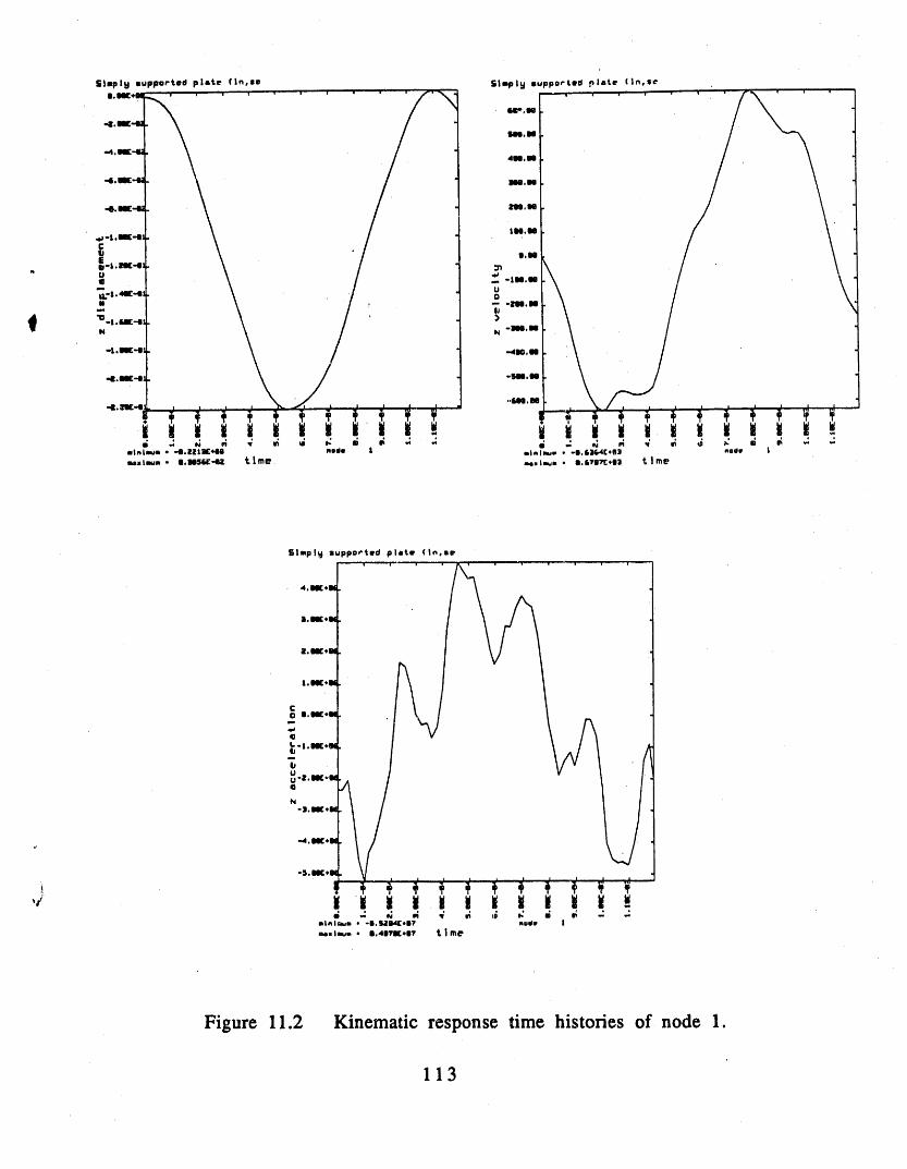
SlspI_ xuppneted plttf (In.xe
C0
L.o
Uu@
N
Figure 11.2 Kinematic response time histories of node 1.
113

Simply luppo_ted plate (tn_ie
Figure 11.3 Time history of axx in element 1.
Simply _uppoeted plate (In,xetime • B.SSBBBi:-83 contour value.A,-|, B9[-0:
conto,e# o( z-displacement B.,I.GgE-EImin.-i_ _[+itO in element ! C_-1.48[-e|
' "- 1.28[-0_
....-..=-747,;;_---_,_,,,0 ,<.-,..,<-.,• -B, 6B[-I_2
_ G--G. G3[-82.... 4.50[-B2
/_l/,/zl--._x_\,i_i -_._ 'I
i_,,itti_',,/ / t\ ',\'{__J',",//i,' i.__
y
dlxp, xcale _lctor , 8. iOf_lriel (defllult)×
Figure 11.4 Contours of z-displacement at t = 0.55 ms.
114

51mpl 9 supported plate (ln,set lme = 0.55000E-03 contour values
A= 7,74E+03contours o_ x-stress B= 1,44E+04m In - 0. 232E+04 1n e ] ement 16 C- 2.11E+04
mex • 0.6t_,-..-.,_ ......-.... _ _j- 2.78E+043.45E+04
' " G- 4.BOE+04
/.; ,_. ..-, _ __ _..,.._ ._, . ._ 5.47E+04
i
___,),,,_ -_._i
d|sp. stele ¢'ector - 0.100E+01 (de.'eult)
Figure 11.5 Contours of Oxx at t = 0.55 ms.
115
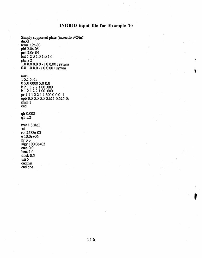
INGRID input file for Example 10
Simplysupportedplate(in,scc,lbs^2/in)dn3dterm1.2c-03plti 2.0c-05pra2._ .o4lcd 1 2 0 1,0 1.0 1.0plane 21.0 0.0 0.0 0 -1 0 0.001 symm
0.0 1.0 0.0-I 0 0.001 symmstart1 5;1 5;-1;0 5.0 0000 5.0 0.0b21 1221001000b 12 122 1001000pr I 1 1 22 11 300.000-1cpb 0.0 0.0 0.0 0.625 0.625 O;mate 1clad
qh O.OOSql 1.2
mat 1 3 shellal
ro .2588c-03c 10.0c+06pr 0,3sigy lO0.Oe+03ctan0.0beta 1.0thick0.5tsti 5cndmatend end
!
116

TAURUS input file for Example 10
reso 1024 1024c Figure 11. lisa hand sketch
c figure 11.2phs2 nodes 1 1 elements 1 1 gather ntime 3 1 1 ntime 6 1 1 ntime 9 1 1
- c Figure 11.3 Shell innercrime 1 1 1
# c Figure 11.4phsl restore razx rayztime 0.55e-03 contour 19
e Figure 11.5contour 1end
_'_
117
Acknowledgements
4
The authors wish to acknowledge the many DYNA3D users who,
over the years, have contributed their models for use as exampleproblems, lt is through interactiov with code users, both inside and
outside LLNL, that the inspiration and material for this manual
originated. In particular, the analysts in the LLNL Applied Mechanics
Group and Advanced Engineering Analysis Group have been especially
generous in sharing their work for the benefit of others. Special
thanks should also be given to Todd Slavik for his thoroughness in
reviewing this manual.
118

References
[1] Hallquist, J. O., and Whirley, R. G., DYNA3D USER'S MANUAL: Nonlinear Dynamic
Analysis of Structures in Three Dimensions, University of California, Lawrence
Livermore National Laboratory, Report UCID-19592, Rev. 5, May, 1989.
[2] Wilkins, M. L., and Guinan, M. W., "Impact of Cylinders on a Rigid Boundary", J.
# of appl. Phys., 44 (1973).
[2] Stillman, D. W., and Hallquist, J. O., INGRID' A Three-Dimensional Mesh
Generator for Modeling Nonlinear Systems, University of California, Lawrence
Livermore National Laboratory, Report UCID-20506, July, 1985.
[3] Rainsberger, R., INGRID by Example: A Pictorial Tutorial, University of
California, Lawrence Livermore National Laboratory, Report UCID-21566,
November, 1988.
[4] Rainsberger, R., INGRID Features and Updates, University of California,
Lawrence Livermore National Laboratory, Report UCID-21620, January, 1988.
[5] Wayne, B., INGRID: Entering Material Specifications, University of California,
Lawrence Livermore National Laboratory, Report UCID-21798, July, 1989.
[6] Brown, B. E., and Hallquist, J. O., TAURUS: An Interactive Post-Processor for the
Analysis Codes NIKE3D, DYNA3D, TACO3D, and GEMINI, University of California,
Lawrence Livermore National Laboratory, Report UCID-19392, Rev. 1, May, 1984.
' [7] Hallquist, J. O., Theoretical Manual for DYNA3D, March, 1983, UniverSity of
California, Lawrence Livermore National Laboratory, pp. 19-20.,ti
119


