CER-ETH - Center of Economic Research at ETH Zurich

Economics Working Paper Series

Eidgenössische Technische Hochschule Zürich

Swiss Federal Institute of Technology Zurich

The Efficiency and Evolution of R&D Networks

Michael D. Konig a S. Battiston a M. Napoletano a,b F. Schweitzer a

aChair of Systems Design, ETH Zurich, Kreuzplatz 5, CH-8032 Zurich, SwitzerlandbObservatoire Francais des Conjonctures Economiques, Department for Research on Innovation and

Competition, 250 rue Albert Einstein, 06560 Valbonne, France

Abstract

This work introduces a new model to investigate the efficiency and evolution of networks of firmsexchanging knowledge in R&D partnerships. We first examine the efficiency of a given networkstructure in terms of the maximization of total profits in the industry. We show that the efficientnetwork structure depends on the marginal cost of collaboration. When the marginal cost is low,the complete graph is efficient. However, a high marginal cost implies that the efficient networkis sparser and has a core-periphery structure. Next, we examine the evolution of the network struc-ture when the decision on collaborating partners is decentralized. We show the existence of mul-tiple equilibrium structures which are in general inefficient. This is due to (i) the path dependentcharacter of the partner selection process, (ii) the presence of knowledge externalities and (iii) thepresence of severance costs involved in link deletion. Finally, we study the properties of the emerg-ing equilibrium networks and we show that they are coherent with the stylized facts of R&D net-works.

Key words: R&D networks, technology spillovers, network efficiency, network formation

JEL classification: D85, L24, O33

1. Introduction

R&D partnerships have become a widespread phenomenon characterizing technologicaldynamics, especially in industries (Hagedoorn, 2002) with rapid technological develop-ment such as, for instance, the pharmaceutical, chemical and computer industries (seeAhuja, 2000; Pammolli and Riccaboni, 2002; Powell et al., 2005; Roijakkers and Hage-doorn, 2006). In those industries, firms have become more specialized on specific domainsof a technology and they tend to combine their knowledge with the one of other firmsthat are specialized in different domains (Ahuja, 2000; Powell et al., 1996).

Email address: mkoenig@ethz.ch (Michael D. Konig).

Preprint submitted to Elsevier 31 August 2008

In this paper, we build a model in which firms innovate by recombining their knowl-edge with that of other firms in the industry, via a network of costly R&D collaborations.Within this framework, we first study the efficiency of a given network structure in termsof maximization of total profits in the industry. We characterize the topology of the effi-cient structure for any level of the marginal cost of collaborations in the relevant range.Next, we study the emergence of pairwise stable structures by employing the notionof “improving path” (cf. Jackson and Watts, 2002), and assuming that link deletionis subject to severance costs. We show the existence of multiple stable structures. Inaddition, we study the relation between network stability and efficiency. Finally, we in-vestigate equilibrium selection under a two-sided myopic link dynamics and we show thatthe model is able to generate stable structures that match the properties of empiricallyobserved R&D networks.

Our research is motivated by two different, albeit related, streams of literature onR&D collaborations. On the one hand, the increasing importance of R&D partnershipshas spurred research, both theoretical and empirical, on the consequences of a givenstructure of the network of R&D collaborations for technology innovation and diffusion(see among many others Ahuja, 2000; Cowan and Jonard, 2004, 2007; Letterie et al.,2008). To this regard, an important and still unsettled debate concerns the relationbetween the position of a firm in the network and its performance, and, in particular,whether a densely interconnected network is more conducive to knowledge diffusion andinnovation than a network with structural holes (i.e. displaying the presence of hubsindirectly connecting many firms which have no direct link across them). Indeed, clustersof densely and directly connected firms might be seen as fostering collaboration effortsamong participants by generating trust and punishment of opportunistic behaviors, anda common language and problem solving heuristics (see e.g. Ahuja, 2000; Coleman, 1988;Cowan and Jonard, 2007; Walker et al., 1997). Conversely, by creating a structural holein the network firms may have access to different sources of knowledge spillovers at thesame time economizing on the costs of direct collaborations (cf. Burt, 1992; Gargiulo andBenassi, 2000; Rowley et al., 2000).

On the other hand, another body of contributions has investigated the salient featuresof empirically observed R&D networks (see e.g. Ahuja, 2000; Fleming et al., 2007; Hanakiet al., 2007; Powell et al., 2005; Roijakkers and Hagedoorn, 2006). These empirical studieshave identified three main structural properties of innovation networks that are invariantacross the different industries examined: (i) Networks are sparse, that is, from all possi-ble connections between firms, only a small subset is realized. (ii) Networks are highlyclustered, that is, they are locally dense. In clusters firms are closely interconnected butbetween different clusters there exist only few connections. (iii) The distribution of linksover the firms tends to be highly heterogeneous with only few firms being connected tomany others. Following this wave of empirical research, theoretical models have exploredthe emergence of R&D networks in a framework with firms being allowed to form anyarbitrary pattern of bilateral R&D agreements (see Goyal and Joshi, 2003; Goyal andMoraga-Gonzalez, 2001, for an equilibrium approach, and Cowan et al., 2006, for anagent-based approach) . However, these models lead to network structures that are toosimple to account for the stylized facts listed above.

Our paper contributes to the foregoing literature along several dimensions. First, weshow that the network structure maximizing industry welfare (measured as the sum offirms’ profits) is a function of the marginal cost of collaborations. In particular, we show

2

that the efficient graph always belongs to a specific class of graphs (the class of nested-split graphs, see Definition (2) and Proposition (3)). Furthermore, when the marginalcost is low the efficient graph graph coincides with the complete graph, i.e. the one maxi-mizing the number of direct ties . As marginal costs increase, it is efficient for the industryto organize into networks having a core-periphery structure. More precisely, at high levelof collaboration costs, efficient networks display the presence of hubs, indirectly linkingcliques of firms to otherwise disconnected nodes in the network. Second, and relatedly, weshow that if marginal collaboration costs and the size of the industry are large enough,the efficient structure for the industry is characterized by significant inequality in prof-its across firms. In particular, firms having less (more) direct connections are also theones displaying higher (lower) profits. In addition, profits inequality increases both inthe number of firms and in the marginal cost of collaboration. Third, we study the rela-tion between efficiency and equilibrium networks in our model. We show that multipleequilibrium structures for the same level of collaboration costs do arise in our model.In particular, we demonstrate that, for the same level of collaboration cost, both thespanning star (i.e. the star encompassing all nodes in the network), as well as the graphcomposed by disconnected cliques of the same size are possible equilibrium networks. Theexistence of multiple equilibria implies that efficiency is not necessarily met by equilib-rium structures in our model. In addition, we identify the conditions on industry size andcollaboration costs under which the efficient network never belongs to the set of possibleequilibria. Finally, we study the properties of equilibrium structures in our model and wecompare them with those of empirical R&D networks. More precisely we investigate theemergence equilibrium structures under a two-sided link formation/deletion mechanism(see Vega-Redondo, 2007, p. 212) in which firms are stochastically selected to revise theircollaboration strategies. In this dynamics, firms decide to form a link if the link did notexist before and the link is beneficial to both of them, and decide to delete a link ifthe link existed before and deletion is beneficial to at least one of the agents selected.We show that under this dynamics the model is able to generate equilibrium structuresmatching the stylized facts of empirical R&D networks.

As we mentioned above, the possibility of recombining different knowledge stocks tointroduce innovations in the industry is the rationale for R&D collaborations in ourmodel (see Ahuja, 2000; Kogut and Zander, 1992; Powell et al., 1996; Weitzman, 1998).We formalize this idea by assuming that the arrival rate of innovations is proportional tothe growth rate in the knowledge stock of the firm, and that firm’s knowledge growth isa linear combination of the idiosyncratic knowledge stocks of the firm and the knowledgeof its R&D partners. In the model, firm’s expected profits are a linear function of theexpected number of innovations per period and of the costs of R&D collaborations.Each R&D collaboration requires a fixed investment over each period. Total costs ofcollaboration are thus proportional to the number of collaborations (the degree) of thefirm. Moreover, if the period over which collaborations are evaluated is long enough, theexpected number of innovations per period turns out to be proportional to the largesteigenvalue of the adjacency matrix associated with the connected component to whichthe firm belongs (see Proposition (1) and Corollary (1)). This has several implications.First, as the largest eigenvalue is the same for all firms in the same component, theformation/deletion of a collaboration by a firm has a strong non-rival external effect onall its direct and indirect neighbors. Second, the magnitude of the change in eigenvalue,resulting from creating/severing a collaboration, varies with the topology of the network

3

and the position of the two firms involved in the collaboration, thus implying a strongpath-dependent character of partner’s choice decisions. Finally, it can be shown thatthe largest eigenvalue is related to the number of all walks connecting firms in a givencomponent. .

Our model can be related to the models in the network formation literature in whichagents face a trade-off between the benefit they get from accessing the network andthe cost of forming links with other agents (see e.g. Bala and Goyal, 2000; Carayolet al., 2008; Haller and Sarangi, 2005; Jackson and Wolinsky, 1996; Vega-Redondo andGoyal, 2007). To this regard, our model shares many similarities and differences withthe “connections” model introduced in Jackson and Wolinsky (1996) and with the linear“two-way flow” model without decay introduced in Bala and Goyal (2000). For instance,similar to both models, the benefit an agent receives from the network derives also fromindirect connections. In addition, such a benefit is non-rival 1 (see in particular Equation(10) and discussion thereafter). However, differently from both models, link deletioninvolves severance costs. Furthermore, differently from Jackson and Wolinsky’s modelthe benefit the agent receives from the network does not only depend on the shortestpath existing between the agent and its direct and indirect neighbors but it accountsfor all possible walks existing among them. Next, differently from Bala and Goyal’slinear model, link-formation is two-sided. In addition, the payoff of the agent does notonly depend on the number of direct and indirect neighbors that can be reached bythe agent with its existing connections, but also on how each neighbor can be reached.Incorporating all walks and severance costs in the network formation process has severalimplications for the results obtained. First, as efficiency is concerned, similar to Jacksonand Wolinsky’s model (and differently from Bala and Goyal’s model) we obtain thatthe complete graph and the empty graph are efficient for, respectively, very low andvery high values of the marginal cost of link formation. By contrast, differently fromboth models, first, the efficient graph for intermediate levels of the marginal cost ofcollaboration (i.e. the nested-split graph), is in general not minimally connected (i.e. morethan one path exists between any two agents in the efficient graph). Second, stable graphsare not necessarily connected as they can consists of several disconnected components.Similar to both models, we obtain the spanning star as possible equilibrium networkfor intermediate levels of marginal cost of collaboration. However, differently from bothmodels, this equilibrium coexists with an equilibrium consisting of the class of graphscomposed of disconnected cliques of the same size.

The paper is organized as follows. Section 2 contains the description of the model,starting with the definition of the network of R&D collaborations across firms, and thenmoving to explain how firms profit from R&D collaborations, and the relations betweenour model and the others proposed in the literature. Section 3 is devoted to the analysisof the efficiency of R&D network structures and to the relation between efficiency andinequality in firms’ profits. Network dynamics, the emergence of equilibrium networksand their properties are analyzed in Section 4. Finally, Section 5 concludes. All proofscan be found in the appendix.

1 See Vega-Redondo and Goyal (2007) for a model where benefits from indirect connections are rival.

4

2. The Model

We consider an industry in which firms engage in pairwise R&D collaborations with otherfirms. Collaborations allow the growth of knowledge within the firm and an increase inthe probability to introduce innovations that yield profits to the firm. We first define thenetwork of R&D collaborations. Next, we characterize how the R&D network influencesknowledge growth, innovation and profits of the firms. Finally, we briefly discuss therelations between our model and the relevant literature.

2.1. The Network

Consider an industry populated by n firms. The network 2 G is the pair (N,E) consistingof the set of nodes N(G) = {1, ..., n}, representing the population of firms and a set ofedges E(G), representing R&D collaborations among the firms 3 (for simplicity we mayjust write N and E where it is obvious to which network G the sets refer). An edgeij ∈ E, represents the existence of an R&D collaboration between firm i and j, which aresaid to be adjacent. A subgraph of G is a pair G′ = (N ′, E′) such that N ′ ⊆ N , E′ ⊆ E.The number of nodes is |N | = n and the number of edges |E| = m. A complete graphKn is a graph in which all n nodes are pairwise adjacent. The graph in which no pair ofnodes is adjacent is the empty graph Kn. A clique Kn′ , n′ ≤ n, is a complete subgraph ofthe network G. In contrast to the clique, an independent set Kn′ is a subgraph in whichall n′ nodes are not pairwise adjacent.

The neighborhood of i is the set Ni = {j ∈ N : ij ∈ E}. The degree of a node i inG, written by di, is the number of edges incident to i. Clearly, di = |Ni|. The maximumdegree is ∆(G) and the minimum degree is δ(G). The clustering coefficient Ci of firm iis the proportion of links between the firms within its neighborhood Ni divided by thenumber of links that could possibly exist between them, i.e.

Ci =2|{jk : j, k ∈ Ni ∧ jk ∈ E}|

di(di − 1). (1)

The total clustering coefficient is the sum of the clustering coefficients for each firm,C =

∑ni=1 Ci.

A walk Wk of length k connecting firm i1 and ik is a sequence of firms (i1, i2, ..., ik) suchthat i1i2, i2i3, ..., ik−1ik ∈ E. A walk is closed if the first and last firm in the sequenceare the same, and open if they are different. A path is a walk in which no firm is visitedtwice. A closed path encompassing n nodes is a cycle, denoted by Cn.

A connected component in G is a maximal set of firms such that there exists a pathbetween any two of them. We will say that two components are disconnected if there isno path between them. A connected graph is a graph consisting of only one connectedcomponent.

Let A(G) be the symmetric n × n adjacency matrix of the R&D network G. Theelement aij ∈ {0, 1} indicates if there exists a link between agent i and j such thataij = 1 if ij ∈ E and aij = 0 if ij /∈ E. The eigenvalues of the adjacency matrix A are

2 In this paper we will use the terms graph and network interchangeably. The same holds for links andedges.3 We consider undirected graphs only.

5

the numbers λ such that Ax = λx has a nonzero solution vector, which is an eigenvectorassociated with λ. The term λPF denotes the largest real eigenvalue of A (the Perron-Frobenius eigenvalue, cf. Horn and Johnson, 1990; Seneta, 2006), i.e. all eigenvalues λof A(G) satisfy |λ| ≤ λPF and there exists an associated nonnegative eigenvector v ≥ 0such that Av = λPFv. For a connected graph G the adjacency matrix A(G) has a uniquelargest real eigenvalue λPF and a positive associated eigenvector v > 0.

Finally, for a graph with n nodes there are(n2

)possible links and accordingly there are

2(n

2) possible graphs on n nodes. We denote with G(n, p) the random graph with n nodes,in which each of the possible links occurs independently with probability p. Similarly,G(n,m) is the random graph with n nodes and m edges.

2.2. Innovation and Profits from R&D Collaborations

Firms exploit R&D collaborations to introduce innovations in the industry. Decisions overR&D partners are taken at discrete times t = T, 2T, 3T, ... where the length of a periodis given by T > 0. Innovations are introduced during each period (t, t + T ]. The rewardsfrom each innovation are assumed to be appropriable so that an innovation returns avalue equal to the constant V > 0. Following the theoretical literature on innovationand endogenous technical change (see e.g. Aghion and Howitt, 1998; Reinganum, 1983,1985; Winter, 1984), we assume that the introduction of innovations by a firm i ∈ N isgoverned by a non-homogeneous Poisson process with arrival rate equal to hi(τ), whereτ ≥ 0 indicates the time variable within a period. Thus, the probability that an innovationis introduced by firm i in the interval dτ , is equal to hi(τ)dτ . Moreover we assume that,for any firm i, the arrival rate of innovations is proportional to the growth rate ρi(τ) ofknowledge 4

hi(τ) = bρi(τ), b > 0. (2)

In other words, the higher the growth rate of knowledge, the more likely it is that the firmwill be able to innovate. Expected revenues of firm i in a period (t, t+T ] are given by thevalue V of each innovation times the expected number of innovations in the period. Notethat in Equation (2) the innovation process starts anew at the beginning of every period(t, t + T ], taking as initial condition the stock of knowledge at the end of the previousperiod (t−1, t−1+T ]. In addition, let us set τ ∈ (0, T ]. From Equation (2) the expectednumber of innovations in a period (t, t + T ] can be written as

∫ T

0

hi(τ)dτ = b

∫ T

0

ρi(τ)dτ. (3)

In turn, the growth rate of knowledge is affected by the network of collaborations asfollows. In each period (t, t+T ], new knowledge is generated by recombining the existingknowledge stocks of firms in the economy via the existing network of R&D collaborations(see Kogut and Zander, 1992; Weitzman, 1998). More precisely, let us denote by xi(τ)the stock of knowledge of firm i at time τ ∈ (t, t + T ]. Then new knowledge within firmi is generated according to:

4 Note that both, the innovation arrival rate hi(τ) and the growth rate of knowledge ρi(τ) are flowvariables and are measured per unit of time.

6

xi(τ) =

n∑

j=1

aij(t)xj(τ), (4)

where aij(t) are the elements of the adjacency matrix A(G(t)) (defined in Section 2.1)corresponding to the network of R&D collaborations 5 . In vector-matrix notation Equa-tion (4) reads x(τ) = A(G(t))x(τ). Note also that in Equation (4) for non-negative initialvalues of x(0) ≥ 0, we have that x(τ) ≥ 0 as well as x(τ) ≥ 0.

The growth rate of knowledge of firm i, ρi(τ) = xi(τ)/xi(τ), in Equation (4) is directlyaffected by the growth rate of knowledge of its neighbors, whose growth rate is affectedby the growth rate of their neighbors, and so on. It turns out that the topology of thewhole network of R&D collaborations (including all direct and indirect paths along whichknowledge can flow between the firms), influences the innovation process within the firm.

Collaborations also imply a cost for firms. Within a period (t, t+T ] each collaborationinvolves a cost per unit of time equal to c. Moreover, we assume that firms are risk-neutral. Finally, if we denote by Gi(t) the connected component to which firm i belongsin the period, then expected profits for the firm at the beginning of the period can bewritten as

πi(Gi(t), c, t) = bV

∫ T

0

ρi(τ)dτ − cT di(t), (5)

where di(t) is the degree of the firm at time t and during the period.The timing of events in each period (t, t + T ] runs as follows: at the beginning t of

the period the network of R&D collaborations is determined (only one link is added orremoved at time t), and remains fixed throughout the period (t, t+T ]. During the period(t, t + T ], firms recombine their knowledge stocks through the network while they alsobear the costs of their collaborations. As a result, innovations are introduced and therents accrue to the firm.

The expression for expected profits in Equation (5) can be directly related to the struc-ture of the network of collaborations. For this purpose, the next proposition establishesa relation between, on one hand, the asymptotic growth rate of ideas, the asymptoticrelative stock of knowledge and the rate of convergence, and, on the other hand, the eigen-values and eigenvectors of the adjacency matrix A(Gi(t)) of the connected componentof firm i.

Proposition 1 Consider the eigenvalues λPF = λ1 ≥ λ2 ≥ ... ≥ λn associated with theadjacency matrix A(Gi(t)) of the connected component Gi(t) of firm i ∈ N(Gi(t)). Thenthe following results hold:

(i) The asymptotic knowledge growth rate of a firm i is constant and equal to the largestreal eigenvalue (Perron-Frobenius eigenvalue) of the adjacency matrix A(Gi(t))

limτ→∞

ρi(τ) = λPF(Gi(t)). (6)

The rate of convergence is O(e−[λPF(Gi(t))−λ2(Gi(t))]τ

)as τ → ∞.

(ii) The asymptotic value of a firm i’s relative knowledge stock equals the element vi ofthe eigenvector associated with the eigenvalue λPF(Gi(t))

5 In Equation (4) we are assuming the process of creation of ideas at the firm level is cumulative, inthat larger knowledge stocks (of the firm and of its collaborators) lead to higher knowledge growth. Thisproperty of knowledge dynamics has often been emphasized in innovation studies (see e.g. Dosi, 1988).

7

limτ→∞

xi(τ)∑n

j=1 xj(τ)= vi. (7)

Item (i) of the above proposition states that the knowledge dynamics defined in Equation(4) converges, for a given R&D network, to a steady state characterized by a constantgrowth rate of ideas. In addition, such a constant growth rate depends on the topologyof the connected component which the firm belongs to (through the largest eigenvalueλPF (Gi(t))). This implies that, in the steady state, the arrival rate of an innovation isconstant and equal to bλPF . Moreover, item (ii) implies that the topology of the connectedcomponent Gi(t) determines the distribution of relative values of the knowledge stocksof firms in the same component. Finally, the rate of convergence to the steady state isdetermined by the eigenvalues of 6 A(Gi).

An important assumption of our model is that the growth of knowledge is much fasterthan the formation of R&D collaborations. This is equivalent to saying that τ is measuredin time units much smaller than those used to measure t. In other words, t = kτ , with klarge. Under this assumption, the expected number of innovations per unit of time canbe approximated (taking the limit k → ∞) with the largest real eigenvalue of a firm’sconnected component.

Corollary 1 The expected number of innovations of firm i per unit of time in a period(t, t + T ] tends to a limit proportional to the largest real eigenvalue of firm i’s connectedcomponent Gi.

limk→∞

b

kT

∫ kT

0

ρi(τ)dτ = bλPF(Gi(t)). (8)

Expected profits of the firm at beginning of the period (t, t + T ] can now be written as

πi(Gi(t), c, t) = bλPF(Gi(t))V T − cdi(t)T. (9)

Applying an affine transformation to the above equation, we finally obtain expectedprofits per unit of time in the period between t and t + T ,

πi(Gi(t), c, t) = λPF(Gi(t)) − cdi(t), (10)

where c = cbV

is the marginal cost of link formation (rescaled by the factor 1/bV ) 7 .Since in Equation (10) the largest eigenvalue λPF(Gi(t)) is the same for all firms in thesame connected component, the expected revenues from R&D collaborations will be thesame for all the members of Gi. Nonetheless, profits from R&D collaborations vary, ingeneral, across firms, since each firm may have a different number of collaborations. Thefollowing lemma 8 characterizes the relation between the largest eigenvalue of a connectedcomponent and the creation or removal of R&D collaborations.

6 In general, the convergence in a connected component to its largest real eigenvalue is always guar-anteed. In addition, more dense networks are characterized by a faster convergence (see the proof of

Proposition (1) in the appendix). However, the convergence can be slow for sparse networks and par-ticular network topologies. For a recent application and discussion of the convergence properties of thesocial network matrices see Jackson and Golub (2007).7 The introduction of linear and homogeneous in-house R&D activities in Equation (4) for the dynamicsof knowledge stocks would not alter the functional form of profits (up to a constant).8 A proof of the foregoing lemma can be found in Cvetkovic et al. (1995).

8

Lemma 1 Denote G′ = (N ′, E′) the graph obtained from the graph G = (N,E) by theaddition or removal of an edge. Then

(i) λPF(G′) ≥ λPF(G) if ij /∈ E and λPF(G′) ≤ λPF(G) if ij ∈ E.(ii) λPF(G′) ≤ λPF(Kn) = n − 1.(iii) |λPF(G′) − λPF(G)| ≤ 1

Thus, the largest real eigenvalue in a component is a non decreasing function of thenumber of links. In addition, it is a bounded function, since its value can never be higherthan the one associated with the complete graph Kn. Finally, the change in the eigen-value is itself a bounded function, since its value must be less than one. The precedingobservations deliver two central properties of the model. First, since the probability ofinnovation is the same for all the firms in a given connected component and it is affectedby each link, the creation (deletion) of a collaboration by one firm has a positive (nega-tive) non-rival external effect on all its direct and indirect neighbors in the component.As we will discuss in Section 4, this property is at the origin of the fact that the net-work can evolve into equilibria that are socially inefficient. Second, the marginal revenuefrom R&D collaborations is always a positive (albeit bounded) function of the numberof links. This means that the creation (deletion) of a new R&D collaboration increases(decreases) the probability of an innovation and thus the expected revenue. Moreover,the revenue itself is a bounded function of the number of links. The last property doesnot imply that the revenue is also a concave function of the number of links 9 . However,as we will show in Section 4, it implies that, as the network grows in the number of links,the highest marginal revenue that can actually be obtained from the creation of a newlink or from the removal of an existing link can become very small. It turns out that,when the highest marginal revenue from a collaboration that can be obtained is smallerthan the marginal cost of collaboration, the network reaches an equilibrium, and thismay happen well before the network has grown to a fully connected graph.

2.3. Relation to the Literature on Network Formation

The profit Equation (10) can be compared to other similar utility functions in the litera-ture that feature a dependence on the position of a firm in the network. For instance, theutility function proposed in the “connections” model in Jackson and Wolinsky (1996) isgiven by

ui =

n∑

j=1

δd(i,j) − cdi, (11)

where 0 < δ < 1 and d(i, j) is the length of the shortest path from node i to node j.The difference between the profit function in (10) and the utility function in (11)

becomes apparent in the benefit term. While Equation (11) considers the shortest pathbetween firm i and j only, our model instead takes into account all possible walks fromfirm i to the other firms in the connected component 10 . Recall that, in our model, a

9 Incidentally, note that λPF is not even determined as a function of m, because, for a given m, thereare many different ways to arrange the links among the nodes, resulting in different values of λPF.10 It has been argued that in several settings paths that are not the shortest may have a big impacton the information that is transmitted from one agent to another (see e.g. Stephenson and Zelen, 1989;Wasserman and Faust, 1994). Moreover, empirical studies on R&D networks (cf. Powell et al., 2005) bring

9

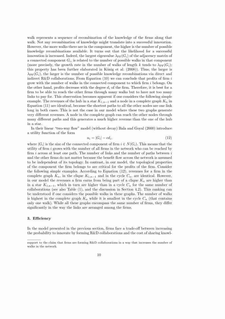
walk represents a sequence of recombination of the knowledge of the firms along thatwalk. Not any recombination of knowledge might translate into a successful innovation.However, the more walks there are in the component, the higher is the number of possibleknowledge recombinations available. It turns out that the likelihood for a successfulinnovation is increased. Indeed, the largest eigenvalue λPF(Gi) of the adjacency matrix ofa connected component Gi, is related to the number of possible walks in that component(more precisely, the growth rate in the number of walks of length k tends to λPF(Gi);this property has been further elaborated in Konig et al. (2008)). Thus, the larger isλPF(Gi), the larger is the number of possible knowledge recombinations via direct andindirect R&D collaborations. From Equation (10) we can conclude that profits of firm igrow with the number of walks in the connected component to which firm i belongs. Onthe other hand, profits decrease with the degree di of the firm. Therefore, it is best for afirm to be able to reach the other firms through many walks but to have not too manylinks to pay for. This observation becomes apparent if one considers the following simpleexample. The revenues of the hub in a star K1,n−1 and a node in a complete graph Kn inEquation (11) are identical, because the shortest paths to all the other nodes are one linklong in both cases. This is not the case in our model where these two graphs generatevery different revenues. A node in the complete graph can reach the other nodes throughmany different paths and this generates a much higher revenue than the one of the hubin a star.

In their linear “two-way flow” model (without decay) Bala and Goyal (2000) introducea utility function of the form

ui = |Gi| − cdi, (12)

where |Gi| is the size of the connected component of firm i ∈ N(Gi). This means that theutility of firm i grows with the number of all firms in the network who can be reached byfirm i across at least one path. The number of links and the number of paths between iand the other firms do not matter because the benefit flow across the network is assumedto be independent of its topology. In contrast, in our model, the topological propertiesof the component the firm belongs to are critical for the profits of the firm. Considerthe following simple examples. According to Equation (12), revenues for a firm in thecomplete graph Kn, in the clique K1,n−1 and in the cycle Cn, are identical. However,in our model the revenues a firm earns from being part of a clique Kn are higher thanin a star K1,n−1, which in turn are higher than in a cycle Cn for the same number ofcollaborations (see also Table (1), and the discussion in Section 4.2). This ranking canbe understood if one considers the possible walks in these graphs. The number of walksis highest in the complete graph Kn while it is smallest in the cycle Cn (that containsonly one walk). While all these graphs encompass the same number of firms, they differsignificantly in the way the links are arranged among the firms.

3. Efficiency

In the model presented in the previous section, firms face a trade-off between increasingthe probability to innovate by forming R&D collaborations and the cost of sharing knowl-

support to the claim that firms are forming R&D collaborations in a way that increases the number ofwalks in the network.

10

edge with other firms in the industry. In this section we investigate how this trade-off canbe managed in order to yield the best outcome from the industry point of view. First,we show that there exists an interval of the marginal cost of link formation, c ∈ [0, 1],in which the network that maximizes social welfare, that is the efficient graph, is a con-nected graph. We will show in Section 4 that this interval is the one of main interestsince for values above this interval, c > 1, firms do not have the incentive to form anyadditional collaboration.

We then investigate the topology of the efficient graph, and we show that it belongsto a well defined class of connected graphs, the “nested split graphs”. In particular,for c small enough, the efficient graph is the complete graph. On the other hand, forhigher values of c and a larger number of firms, the efficient graph is sparser and showsa strong degree heterogeneity. In addition, we show that it is characterized by significantinequality in profits.

3.1. Efficient Networks

Following Jackson and Wolinsky (1996), we define industry welfare as the sum of firms’individual profits

Π(G, c) =∑n

i=1 πi(Gi)

=∑n

i=1 (λPF(Gi) − cdi)

=∑n

i=1 λPF(Gi) − 2mc.

(13)

We are interested in the solution of the following social planner’s problem. Let G(n)denote the set of all possible graphs with n nodes. For a given value of cost c, the socialplanner’s solution is given by

G∗ = argmaxG∈G(n)

Π(G, c). (14)

A graph G∗ solving the maximization problem (14), will be denoted as “efficient”.Inorder to solve this problem we begin by identifying an interval for the marginal costs cin which industry welfare is increased by connecting two disconnected components of thenetwork. The following lemma can be stated.

Lemma 2 Consider a graph G consisting of two disconnected components G1 and G2,with n1, n2 nodes, m1, m2 edges, eigenvalues λPF(G1), λPF(G2) and total profits Π(G1) =n1λPF(G1)−2m1c, Π(G2) = n2λPF(G2)−2m2c. We further assume that c ∈ [0, 1]. Thenthere exists a connected graph G′ with n = n1 + n2 nodes that has higher total profitsthan G, that is Π(G′) ≥ Π(G) = Π(G1) + Π(G2).

Thus, for c ∈ [0, 1], connecting two previously disconnected components of the graphyields total profits larger than the respective total profits of the disconnected components.From this it follows immediately that the efficient network is connected.

Proposition 2 Let H(n,m) denote the set of connected graphs having n nodes and mlinks. If c ∈ [0, 1] then G∗ ∈ H(n,m).

This means that, in order to guarantee efficiency, each firm must have (direct or indirect)access to the knowledge of all other firms in the industry.

11

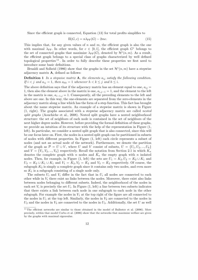
Since the efficient graph is connected, Equation (13) for total profits simplifies to

Π(G, c) = nλPF(G) − 2mc. (15)

This implies that, for any given values of n and m, the efficient graph is also the onewith maximal λPF. In other words, for c ∈ [0, 1], the efficient graph G∗ belongs tothe set of connected graphs that maximize λPF(G), denoted by H∗(n,m). As a result,the efficient graph belongs to a special class of graphs characterized by well definedtopological properties 11 . In order to fully describe these properties we first need tointroduce some basic definitions.

Brualdi and Solheid (1986) show that the graphs in the set H∗(n,m) have a stepwiseadjacency matrix A, defined as follows:

Definition 1 In a stepwise matrix A, the elements aij satisfy the following condition.If i < j and aij = 1, then ahk = 1 whenever h < k ≤ j and h ≤ i.

The above definition says that if the adjacency matrix has an element equal to one, aij =1, then also the element above in the matrix is one, ai,j−1 = 1, and the element to the leftin the matrix is one, ai−1,j = 1. Consequently, all the preceding elements to the left andabove are one. In this way, the one-elements are separated from the zero-elements in theadjacency matrix along a line which has the form of a step function. This fact has broughtabout the name stepwise matrix. An example of a stepwise matrix is shown in Figure(1, right). The graphs associated with a stepwise adjacency matrix are called nestedsplit graphs (Aouchiche et al., 2008). Nested split graphs have a nested neighborhoodstructure: the set of neighbors of each node is contained in the set of neighbors of thenext higher degree nodes. However, before providing the formal definition of these graphs,we provide an intuition of its structure with the help of the representation in Figure (1,left). In particular, we consider a nested split graph that is also connected, since this willbe our focus later on. First, the nodes in a nested split graph can be partitioned in subsetsof nodes with different properties. In Figure (1, left) each circle represents a subset ofnodes (and not an actual node of the network). Furthermore, we denote the partitionof the graph as P = U ∪ V , where U and V consist of subsets, U = {U1, U2, ..., Uk}and V = {V1, V2, ..., Vk} respectively. Recall the notation from Section 2.1 in which Kn

denotes the complete graph with n nodes and Kn the empty graph with n isolatednodes. Then, for example, in Figure (1, left) the sets are U1 = K2, U2 = K2 ∪ K1 andU3 = K2 ∪ K1 ∪ K1 and V1 = K2, V2 = K2 and V3 = K2 respectively. Of course, thesubgraph K2 is simply a complete graph since it contains only two nodes, and even moreso K1 is a subgraph consisting of a single node only.

The subsets Ui and Vi differ in the fact that in Ui all nodes are connected to eachother while in Vi there exist no links between the nodes. Moreover, there exist also linksbetween nodes belonging to different subsets. Indeed, the neighborhood of the nodes ineach set Vi is precisely the set Ui. In Figure (1, left) a line between two subsets indicatesthat there exists a link between each node in one subgraph to each node in the othersubgraph. For example the nodes in V1 at the top right of the figure are all connected tothe nodes in U1 at the top left. Similarly, the nodes in V2 are connected to the nodes inU2 and the nodes in V3 are connected to the nodes in U3. Additionally, the set U as well

11The efficient networks are similar to those obtained in the model of Ballester et al. (2006). Moreprecisely, within that model Corbo et al. (2006) show that the networks that maximize welfare are givenby the graphs with maximal eigenvalue.

12

K2

V1

d = 2

K2

V2

d = 3

K2

V3

d = 4K1d = 5

K1d = 7

K2d = 9

U1

U2

U3

Fig. 1. Representation of a connected nested split graph (left) and the associated adjacency matrix(right) with n = 10 nodes. A nested split graph can be partitioned into subsets of nodes with the samedegree (each subset is represented as circle, the degree d of the nodes in the subset is indicated). A line

connecting two subsets indicates that there exists an edge between each node in one set and all thenodes in the other set. The boxes around the sets indicate the cliques U1 = K2, U2 = K2 ∪ K1 andU3 = K2 ∪ K1 ∪ K1. In the matrix to the right the zero-entries are separated from the one-entries by astepfunction.

as any union of the subsets in U form a complete subgraph or clique. Similarly, any unionof the sets in V form an independent set. Notice also, that all the nodes in one set havethe same degree. Next to the sets in Figure (1, left) the degree of the nodes in a subset isindicated. The degree of a node in a set can be easily derived from the adjacency matrixshown in Figure (1, right) by counting the number of ones in a row corresponding to aparticular node in a set. For example the set K2, top left in the figure, corresponds totwo nodes whose links are indicated in the first two rows of the adjacency matrix.

With the preceding discussion in mind, we can now give a more formal definition of anested split graph(see Cvetkovic et al., 2007).

Definition 2 In a nested split graph, the set of nodes have a partition P = U ∪ V withthe following properties.

(i) U induces a clique, and V induces an independent set. This also holds for anyunion of subsets in U and V .

(ii) U has subsets U1, ..., Uk such that U1 ⊃ ... ⊃ Uk and the neighborhood of each nodein Vi is Ui, for any i = 1, ..., k.

If a nested split graph is connected we call it a connected nested split graph. As we men-tioned above, the representation and the adjacency matrix shown in Figure (1) actuallyshow a connected nested split graph. From the stepwise property of the adjacency matrixit follows that a connected nested split graph contains at least one spanning star, thatis, there is at least one node that is connected to all other nodes. This property can alsobe seen in Figure (1), where the first row of the adjacency matrix that is entirely filledwith ones indicates the presence of a spanning star 12 .

We have shown that G∗ is connected and we know that G∗ has a stepwise adjacencymatrix. From the above discussion we can further conclude that G∗ is a connected nestedsplit graph and it contains at least one spanning star as a subgraph.

12A related type of graph, so called inter-linked stars, has been introduced by Goyal and Joshi (2003).However, this notion does not specify the nested neighbourhood structure that characterizes nested splitgraphs.

13

The determination of the exact topology of G∗, for given n and c, is simple for c ∈[0, 1/2] (see Proposition 3). In contrast, for c > 1/2 this problem requires the determina-tion of the graph with the largest eigenvalue among all graphs in H∗(n,m) (for a fixed nand arbitrary m, with n−1 ≤ m ≤ n(n−1)/2). This is still an unresolved research prob-lem in Spectral Graph Theory (Aouchiche et al., 2008). However, it turns out that thevalue of total profits associated with the efficient graph G∗ can be approximated by thetotal profits associated with a special type of a connected nested split graph. FollowingBell (1991) we denote this graph by Fn,d.

Definition 3 Fn,d is the graph obtained from the complete graph Kd with d nodes anda subset of n − d disconnected nodes, by adding n − d links connecting one node in Kd

to each of the n − d disconnected nodes.

Notice that the complete graph and the spanning star are particular cases of connectednested split graphs (and of the graph Fn,d): the star is K1,n = Fn,1 and the completegraph is Kn = Fn,n. Figure (3) shows several examples of this type of graph for n = 10.

Moreover, the number of edges in Fn,d is given by m =(d2

)+ (n − d).

As discussed in more detail in the proof of the next proposition, the maximum relativediscrepancy of total profits between Fn,d and the efficient graph G∗ is considerably smalland vanishes for large n. For example with n = 100 we get get an error below 2%, whilefor n = 200 the error is below 1% (see also Figure 4 top left). The higher is the numbern of firms, the more total profits of Fn,d get close to total profits of G∗. Thus, in orderto determine the efficient network G∗, if n is small one can search through all connectednested split graphs and identify the one with highest total profits, while for large n, onecan use Fn,d as a good approximation.

Bringing the above results together, we can state the following proposition which char-acterizes the topology of the efficient graph G∗ with n firms in the industry as a functionof the marginal cost of collaboration c ∈ [0, 1].

Proposition 3 Let G∗ be the efficient graph for a given number n of firms and Fn,d bethe graph introduced in Definition (3).

(i) If c ∈ [0, 1] then G∗ is a connected nested split graph.(ii) Denote the relative error in total profits between the the efficient graph and the

graph Fn,d as ǫ = (Π(G∗) − Π(Fn,d))/Π(Fn,d). If c ∈ [0, 1], then the relative erroris bounded from above as follows

ǫ ≤ 2c(2c − 1)n − 5c2

n2 + 2c(1 − 2c)n + 9c2, (16)

and vanishes for large n, i.e. limn→∞ ǫ = 0.(iii) If c ∈ [0, 0.5] then G∗ is the complete graph Kn.(iv) If c > n then G∗ is the empty graph Kn.

Figure (2) gives a graphical representation of the results on network efficiency in Propo-sition (3). In Figure (3) the efficient graphs for values of cost c ∈ [0, 1] and system sizen = 10 are shown 13 . We observe that, with increasing marginal cost, the efficient net-work becomes more sparse and the degree heterogeneity is increasing. For any value of

13For the particular case of n = 10 the connected graph with maximal eigenvalue is known (Aouchicheet al., 2008) and so is the efficient network G∗. In this case, the efficient graph is Fn,d itself (withoutany approximation).

14

0 0.5 1c

Kn

connected nested

split graph

K

K

KK

K

K

∼n→∞

Fn,d

Fig. 2. Illustration of the range of efficient graphs as a function of the cost of collaboration. For costs0 ≤ c ≤ 0.5 the efficient graph is the complete graph Kn. In the region 0.5 < c ≤ 1 the efficient graph is a

connected nested split graph. As indicated in the figure, for n large, Fn,d can be seen as an approximationof G∗ (with a vanishing relative error in total profits).

cost larger than 0.5 the efficient network consists of a densely connected cluster (clique)and one node that acts as a hub (star) and connects the remaining nodes to the cluster.

0.5 0.65 0.75 0.85c

F10,10 = K10 F10,9 F10,8 F10,7

Fig. 3. Efficient graphs for values of cost c = 0.5, 0.65, 0.75, 0.85 and n = 10. The density of the efficientgraph is decreasing and the degree heterogeneity is increasing with increasing cost.

If we consider Fn,d as the efficient network, we can make the following observation.From the topological structure of Fn,d it follows that, when marginal cost of link forma-tion is high, it is efficient to concentrate knowledge creation in a small and dense clusterwith one firm acting as a hub that connects all the peripheral firms to the cluster. As themarginal cost of link formation decreases, knowledge recombination becomes cheaper 14

and it is efficient that a larger fraction of firms takes part in the densely connected clus-ter. Finally, in the region of small marginal cost, 0 ≤ c ≤ 0.5, it is efficient that all firmstake part in a densely connected cluster, therewith establishing as many collaborationsas possible. In this case, the fully connected graph encompassing all firms is the one inwhich total profits in the industry attain their highest possible value.

14Note that for c = 0 the problem in (14) can be reduced to the problem of maximizing total knowledgegrowth in the steady state for a given number of firms, in which case the complete graph is the solution.

15

An important final remark concerns the relation to the efficient graphs found in modelsakin to ours. Similar to both Jackson and Wolinsky (1996) and Bala and Goyal (2000),we find that the efficient graph is always connected and that it includes, depending onthe cost c, the star and the complete graph. However, differently from the model of Balaand Goyal, the efficient graph is in general not minimally connected (removing one linkdoes not necessarily make the graph disconnected). Moreover, differently from the modelof Jackson and Wolinsky, in our model the set of efficient graphs is not limited to thestar and the complete graph, but it includes a whole class of graphs that can be seen asintermediate graphs between these two extreme cases.

3.2. Efficiency and Profits Distribution

Former works on R&D networks (see Cowan and Jonard, 2004) have emphasized theemergence of a trade-off between efficiency (in terms of knowledge diffusion) and in-equality (in terms of knowledge levels). A similar trade-off between efficiency and profitsinequality emerges also in this model if the marginal cost of link formation and the num-ber of firms operating in the industry are high enough. We measure inequality in profitsin terms of profit variance.

In Proposition (2) we have shown that for c ∈ [0, 1] the efficient graph is connected,G∗ ∈ H(n, k). Thus, the returns from collaborations in an efficient graph are identical forall firms (since they have the same largest real eigenvalue) but the cost is different andis proportional the degree of the firm. More formally, let us define by σ2

π the variance ofprofits associated with the graph G. It follows for a graph G ∈ H(n,m) that

σ2π(G) = c2σ2

d(G), (17)

where σ2d is the degree variance. Since degree is by definition homogeneous in a complete

graph, from Proposition (3) it follows that for c ≤ 0.5 profits inequality is zero, and notension between efficiency and equality arises.

For higher values of costs, we can take Fn,d as a sufficient approximation to the efficientnetwork G∗, and from the properties of Fn,d we can conclude that the efficient network ischaracterized by considerable degree heterogeneity and profits inequality. More precisely,the following proposition can be stated.

Proposition 4 Let Fn,d be the graph defined in (3) and d = 2m/n the average degree.Then

(i) The degree variance is growing quadratically with the number of firms, i.e.

σ2d(Fn,d) = O(n2). (18)

(ii) Let c > 0.5. For large n the coefficient of variation of degree, cv(Fn,d) = σd(Fn,d)/d,tends to a constant depending on the cost,

limn→∞

cv(Fn,d) =√

2c − 1. (19)

(iii) Consider the random graph G(n,m) with n nodes and m links. For large n, thedegree variance of the graph Fn,d is larger by a factor n than the variance of arandom graph with equal number of nodes and links

σ2d(Fn,d)/σ2

d(G(n,m)) = O(n). (20)

16

0.5 0.6 0.7 0.8 0.9 10

0.5

1

1.5

2

2.5

3

3.5

4 n = 50

n = 100

n = 200

c

ǫ%

0.5 0.6 0.7 0.8 0.9 10

0.2

0.4

0.6

0.8

1n = 50

n = 100

n = 200

c

c v(F

n,d

)

√2c − 1

0.5 0.6 0.7 0.8 0.9 10

1000

2000

3000

4000

5000n = 50

n = 100

n = 200

c

σ2 d(F

n,d

)

0.5 0.6 0.7 0.8 0.9 1

20

40

60

80

100n = 50

n = 100

n = 200

c

σ2 d(F

n,d

)/σ

2 d(G

(n,m

))

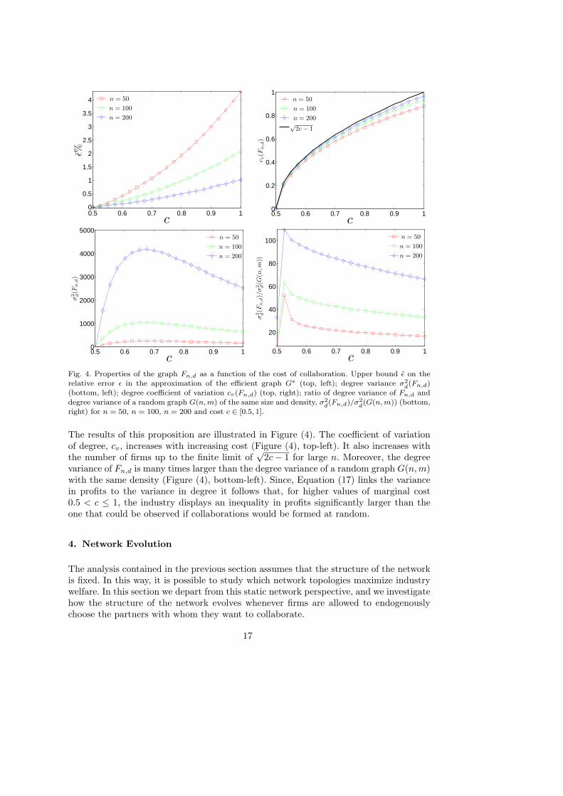
Fig. 4. Properties of the graph Fn,d as a function of the cost of collaboration. Upper bound ǫ on therelative error ǫ in the approximation of the efficient graph G∗ (top, left); degree variance σ2

d(Fn,d)

(bottom, left); degree coefficient of variation cv(Fn,d) (top, right); ratio of degree variance of Fn,d anddegree variance of a random graph G(n, m) of the same size and density, σ2

d(Fn,d)/σ2

d(G(n, m)) (bottom,

right) for n = 50, n = 100, n = 200 and cost c ∈ [0.5, 1].

The results of this proposition are illustrated in Figure (4). The coefficient of variationof degree, cv, increases with increasing cost (Figure (4), top-left). It also increases withthe number of firms up to the finite limit of

√2c − 1 for large n. Moreover, the degree

variance of Fn,d is many times larger than the degree variance of a random graph G(n,m)with the same density (Figure (4), bottom-left). Since, Equation (17) links the variancein profits to the variance in degree it follows that, for higher values of marginal cost0.5 < c ≤ 1, the industry displays an inequality in profits significantly larger than theone that could be observed if collaborations would be formed at random.

4. Network Evolution

The analysis contained in the previous section assumes that the structure of the networkis fixed. In this way, it is possible to study which network topologies maximize industrywelfare. In this section we depart from this static network perspective, and we investigatehow the structure of the network evolves whenever firms are allowed to endogenouslychoose the partners with whom they want to collaborate.

17

Following Jackson and Wolinsky (1996) we consider a network formation process inwhich the creation of a new link requires the bilateral agreement of the two partiesinvolved. However, the deletion of a link requires the unilateral decision of one of thetwo firms only. Consistently, as network equilibrium criterion, we adopt the definition ofpairwise stability, as in Jackson and Wolinsky (1996). Based on this definition of stability,we derive the conditions on the value of cost for which structures like the empty graph,the complete graph or the star are stable. Among the possible stable graphs, we find alsoa disconnected graph consisting of multiple cliques of the same size. A first importantfinding here is the co-existence of multiple equilibrium networks for the same value ofcost.

However, these relatively simple structures are not the only stable networks emergingin our model. Since it is increasingly difficult to derive general proofs of stability for morecomplex structures, we follow the argument in Vega-Redondo (cf. 2007, p. 208) and weperform a dynamic study of network stability. We model explicitly the evolution processin which, at the beginning of each period, a pair of firms decides whether to form ordelete a link, based on the expected profits this action brings about. This investigation,performed through computer simulation, shows that there exist a multitude of complexstructures which are pairwise stable. Remarkably, these networks display topologicalproperties that are consistent with the stylized facts of R&D networks in a region of theparameters of the model.

4.1. Improving Paths and Equilibrium Networks

We consider a process of network evolution in which firms form or delete one link at atime based on the marginal profits they expect from that action. In other words, newlinks are created whenever the increase in the probability of innovation, i.e. the marginalrevenue of a new collaboration, is greater than the marginal cost of a collaboration, withthe gain being strict for at least one of the firms in the selected pair. Likewise, linkdeletion occurs whenever the saving in marginal cost from removing a collaboration areenough to compensate for the decrease in marginal revenue. However, given its unilateralnature, we assume that removing a collaboration involves severance costs 15 so that thesavings in marginal costs from removing a collaboration is reduced by a factor α.

Following Jackson and Watts (2002), we call improving path, a sequence of networks{G(t)}t∈N+

such that (i) any two consecutive networks, G(t) and G(t + 1), differ by onelink only, (ii) if the link is added, both firms benefit from the new link, at least one ofthem strictly, and (iii) if a link is deleted, at least one of the two firms strictly benefitfrom the deletion .

Improving paths emanating from any initial network must either lead to an equilibriumnetwork structure, in which no pair of firms has an incentive to form a link, and no singlefirm has an incentive to remove a link, or to a cycle, in which a finite number of networksis repeatedly visited (see Lemma (1) in Jackson and Watts, 2002). In this section weinvestigate the existence of both equilibrium networks and cycles.

15These severance costs can be associated with the legal procedures needed to unilaterally bring acontract to an end, or it can have a different nature, e.g. they can be associated with the loss ofreputation for managers breaking long-lasting collaborations.

18

Let G denote the current graph G(t) at time t. Further, denote by G + ij the graphobtained from G by adding the edge ij. Similarly, let G−ij denote the graph obtained byremoving the edge ij. Denote by λi(G) the largest eigenvalue λPF(Gi) of the connectedcomponent Gi to which the firm i belongs. Note that, although link deletion implies thatthe degree of i is reduced by one (and so is the cost for firm i), the firm saves only afraction of the cost due to the presence of the severance costs v(c) = (1−α)c. Thus, thechange in profits of firm i induced by the removal of a link are given by:

πi(G − ij) − πi(G) = λi(G − ij) − (di − 1)c − v(c) − (λi(G) − dic)

= c − v(c) − (λi(G) − λi(G − ij))

= αc − (λi(G) − λi(G − ij))

(21)

where α ∈ [0, 1]. Obviously, the firm will only remove a link if this action increases herprofits. With the above notation we can now give the definition of a pairwise stablenetwork.

Definition 4 The graph G is pairwise stable if

(i) ∀ij ∈ E(G), πi(G) ≥ πi(G − ij) and πj(G) ≥ πj(G − ij) or, equivalently, ∀ij ∈E(G), λi(G) − λi(G − ij) ≥ αc and λj(G) − λj(G − ij) ≥ αc

(ii) ∀ij /∈ E(G), if πi(G + ij) > πi(G) then πj(G + ij) < πj(G), and, if πj(G + ij) >πj(G) then πi(G+ij) < πi(G) or, equivalently, ∀ij /∈ E(G), if λi(G+ij)−λi(G) > cthen λj(G+ij)−λj(G) < c, and, if λj(G+ij)−λj(G) > c then λi(G+ij)−λi(G) < c

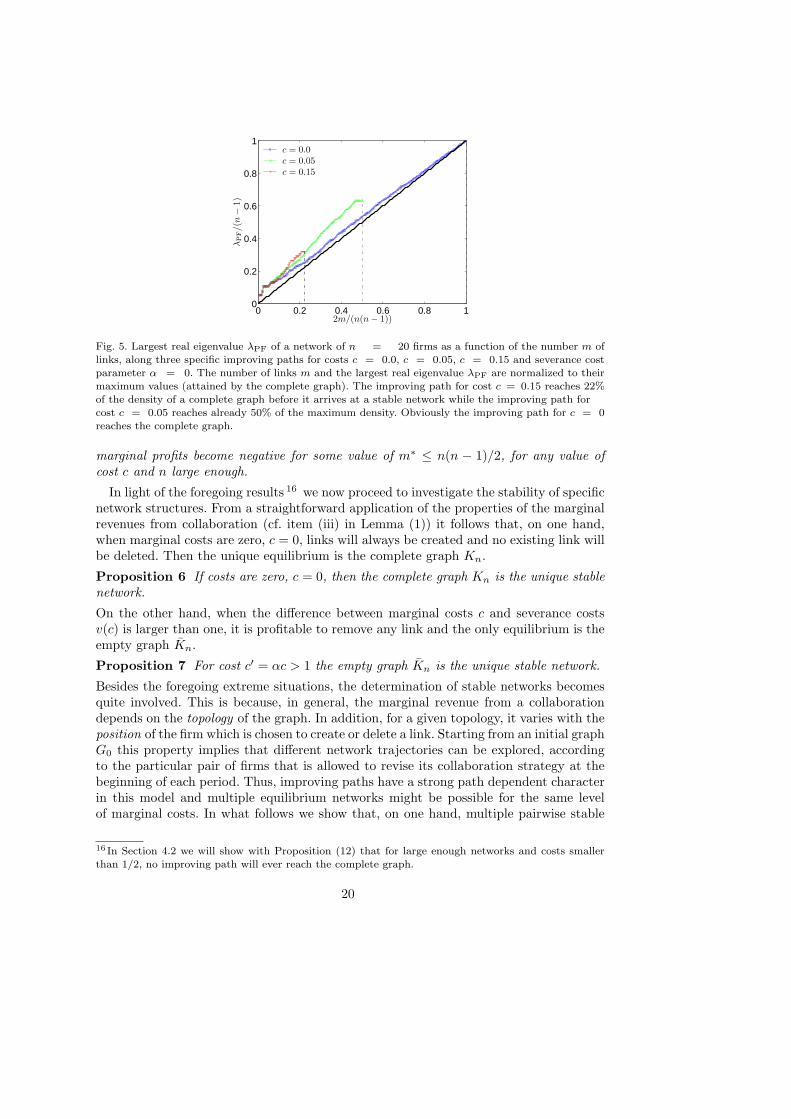
Before moving to the analysis of the existence of stable graphs, we give an explanationabout why in our model the network might stop evolving along an improving path andfinally reach an equilibrium. Let us consider an improving path along which the numberm of links is increasing from m1 = 0, corresponding to the empty graph, to at mostm2 = n(n − 1)/2, corresponding to the complete graph Kn. Figure (5) shows someinstances of improving paths and their corresponding densities (in terms of the numberof links) for different values of the cost c, but with severance cost α = 0. Note thata vanishing value of α implies that no links are removed since then the severance costexceeds any potential gains that could be realized by saving the cost for that link .

For comparison, the figure shows also the straight line with slope 2n, equal to the

average increase of λPF going from the empty graph to the complete graph. In contrast,along any improving path the trajectory of λPF(m) starts off above such straight line.This is stated in the following Lemma and has an important implication.

Lemma 3 Along any improving path in which the number m of links is increasing,λPF(m) increases with m faster than 2

n, in a set of integers I = {0, 1, 2, ...,m0} with

m0 < n(n − 1)/2.

Since, in addition, the sum of the increments of λPF(m) has to be constant (cf. Lemma(1), item (ii)), this means that any improving path has to cross the straight line atsome point before reaching the complete graph. In other words, for some value of m themarginal revenue becomes smaller than the marginal cost (for any value of cost and nlarge enough), implying that the evolution stops. This is stated more precisely in thefollowing proposition.

Proposition 5 Along an improving path in which the number m of links increases,

19

0 0.2 0.4 0.6 0.8 10

0.2

0.4

0.6

0.8

1

λP

F/(

n−

1)

c = 0.0c = 0.05c = 0.15

2m/(n(n − 1))

Fig. 5. Largest real eigenvalue λPF of a network of n = 20 firms as a function of the number m oflinks, along three specific improving paths for costs c = 0.0, c = 0.05, c = 0.15 and severance costparameter α = 0. The number of links m and the largest real eigenvalue λPF are normalized to their

maximum values (attained by the complete graph). The improving path for cost c = 0.15 reaches 22%of the density of a complete graph before it arrives at a stable network while the improving path forcost c = 0.05 reaches already 50% of the maximum density. Obviously the improving path for c = 0

reaches the complete graph.

marginal profits become negative for some value of m∗ ≤ n(n − 1)/2, for any value ofcost c and n large enough.

In light of the foregoing results 16 we now proceed to investigate the stability of specificnetwork structures. From a straightforward application of the properties of the marginalrevenues from collaboration (cf. item (iii) in Lemma (1)) it follows that, on one hand,when marginal costs are zero, c = 0, links will always be created and no existing link willbe deleted. Then the unique equilibrium is the complete graph Kn.

Proposition 6 If costs are zero, c = 0, then the complete graph Kn is the unique stablenetwork.

On the other hand, when the difference between marginal costs c and severance costsv(c) is larger than one, it is profitable to remove any link and the only equilibrium is theempty graph Kn.

Proposition 7 For cost c′ = αc > 1 the empty graph Kn is the unique stable network.

Besides the foregoing extreme situations, the determination of stable networks becomesquite involved. This is because, in general, the marginal revenue from a collaborationdepends on the topology of the graph. In addition, for a given topology, it varies with theposition of the firm which is chosen to create or delete a link. Starting from an initial graphG0 this property implies that different network trajectories can be explored, accordingto the particular pair of firms that is allowed to revise its collaboration strategy at thebeginning of each period. Thus, improving paths have a strong path dependent characterin this model and multiple equilibrium networks might be possible for the same levelof marginal costs. In what follows we show that, on one hand, multiple pairwise stable

16 In Section 4.2 we will show with Proposition (12) that for large enough networks and costs smallerthan 1/2, no improving path will ever reach the complete graph.

20

networks exist for the same value of marginal cost c ∈ (0, 1) and severance costs v(c).On the other hand, we identify a region of costs in the same interval in which stablenetworks do not exist and a sequence of networks is repeatedly visited 17 . In the followingproposition, we show that a set of disconnected cliques of the same size can be a stablenetwork, if their size falls within a certain interval that depends on the marginal cost ofcollaboration c and on the severance cost parameter α.

Proposition 8 Consider costs c, c′ = αc and α ∈ [0, 1]. If the network G consists of aset of k equally sized, disconnected cliques K1

n,K2n, ...,Kk

n (G having kn nodes in total)then G is stable if 18

⌈1 + c(1 − c)

c⌉ ≤ n ≤ ⌊2 − c′(1 − c′)

c′⌋. (22)

From Proposition (8) it follows immediately that for a given value of cost c there existmultiple integer values n (the size of the clique) that fit into the interval spanned by theupper and lower bounds in Equation (8). This is discussed in more details in the proofof Proposition (8) (see appendix) and implies that multiple equilibrium networks existfor a given value of marginal cost c and severance cost v(c).

Moreover, note that the homogeneous size of the cliques is only a sufficient condition forstability but it is not necessary. Indeed, the equilibrium networks obtained with computersimulations show clearly that there exist also equilibria with disconnected cliques ofdifferent sizes (see e.g. Figure (9), bottom-right). The requirement of having cliques ofthe same size appears in Proposition (8) only to allow for an analytical treatment.

Equally sized disconnected cliques are not the only possible stable networks structuresin the interval c ∈ (0, 1) and α ∈ [0, 1]. The next proposition shows that the spanningstar, i.e. the star encompassing all nodes, can be pairwise stable as well, if the size ofthe star (and therewith the number of firms in the industry) falls within a certain regionthat depends on the cost c and on the severance cost parameter α.

Proposition 9 Consider costs c, c′ = αc, α ∈ [0, 1]. The network G consisting of a

spanning star K1,n−1 with ⌈ 2c⌉ ≤ n ≤ ⌊ 1+c′2(6+c′2)

4c′2⌋ is stable.

The foregoing results have two important implications in relation to the literature. First,stable graphs are not necessarily connected. Second, in general they are not minimallyconnected. Indeed, the multiple clique equilibrium is a disconnected graph in which eachcomponent is complete and thus not minimally connected. This is an important featurethat for instance distinguishes our model from the “connections” model in Jackson andWolinsky (1996) and from the linear “two-way flow” model Bala and Goyal (2000). Inboth such models, the equilibrium networks are always connected, while in the latter theyare also minimally connected. Furthermore, both models find that the spanning star isstable for intermediate values of the cost of collaboration. However, differently from bothmodels, in our model the spanning star is never the unique stable network. Indeed,the next proposition combines together the results of the previous two propositions, theconditions under which the link formation dynamics defined in (5) may lead to twodifferent pairwise stable network topologies for the same level of marginal cost c and

17This is a cycle in the space of network trajectories, to not confuse with the specific graph called cycle.18 In the following, ⌈x⌉, where x is a real valued number x ∈ R, denotes the smallest integer larger orequal than x (the ceiling of x). Similarly, ⌊x⌋ the largest integer smaller or equal than x (the floor of x).

21

0.05 0.1 0.15 0.2 0.25 0.3 0.350

20

40

60

80

100

120 α=0.1α=0.5α=1.0

c

num

.st

able

cliq

ue-

size

s

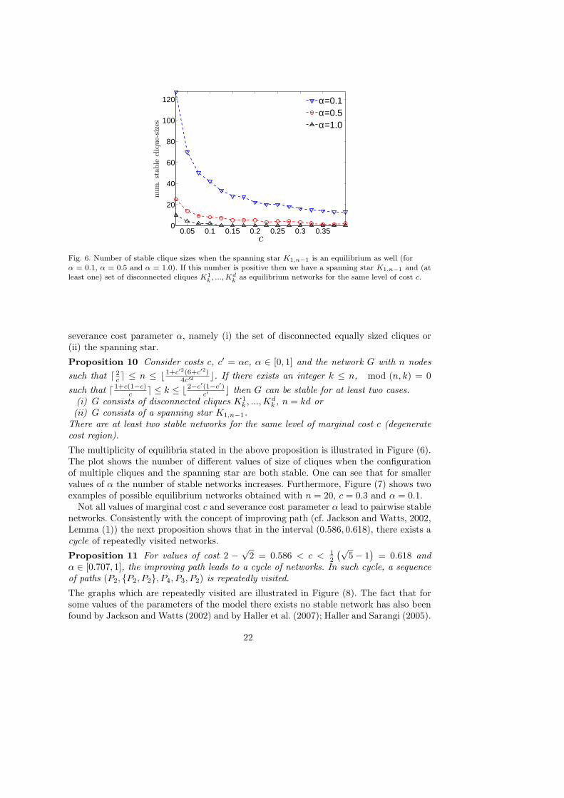
Fig. 6. Number of stable clique sizes when the spanning star K1,n−1 is an equilibrium as well (forα = 0.1, α = 0.5 and α = 1.0). If this number is positive then we have a spanning star K1,n−1 and (atleast one) set of disconnected cliques K1

k, ..., Kd

kas equilibrium networks for the same level of cost c.

severance cost parameter α, namely (i) the set of disconnected equally sized cliques or(ii) the spanning star.

Proposition 10 Consider costs c, c′ = αc, α ∈ [0, 1] and the network G with n nodes

such that ⌈ 2c⌉ ≤ n ≤ ⌊ 1+c′2(6+c′2)

4c′2⌋. If there exists an integer k ≤ n, mod (n, k) = 0

such that ⌈ 1+c(1−c)c

⌉ ≤ k ≤ ⌊ 2−c′(1−c′)c′

⌋ then G can be stable for at least two cases.(i) G consists of disconnected cliques K1

k , ...,Kdk , n = kd or

(ii) G consists of a spanning star K1,n−1.There are at least two stable networks for the same level of marginal cost c (degeneratecost region).

The multiplicity of equilibria stated in the above proposition is illustrated in Figure (6).The plot shows the number of different values of size of cliques when the configurationof multiple cliques and the spanning star are both stable. One can see that for smallervalues of α the number of stable networks increases. Furthermore, Figure (7) shows twoexamples of possible equilibrium networks obtained with n = 20, c = 0.3 and α = 0.1.

Not all values of marginal cost c and severance cost parameter α lead to pairwise stablenetworks. Consistently with the concept of improving path (cf. Jackson and Watts, 2002,Lemma (1)) the next proposition shows that in the interval (0.586, 0.618), there exists acycle of repeatedly visited networks.

Proposition 11 For values of cost 2 −√

2 = 0.586 < c < 12

(√5 − 1

)= 0.618 and

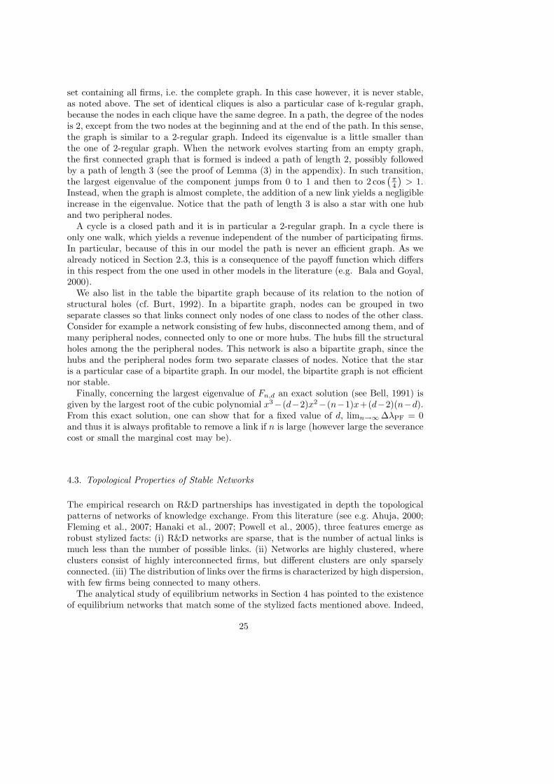
α ∈ [0.707, 1], the improving path leads to a cycle of networks. In such cycle, a sequenceof paths (P2, {P2, P2}, P4, P3, P2) is repeatedly visited.

The graphs which are repeatedly visited are illustrated in Figure (8). The fact that forsome values of the parameters of the model there exists no stable network has also beenfound by Jackson and Watts (2002) and by Haller et al. (2007); Haller and Sarangi (2005).

22

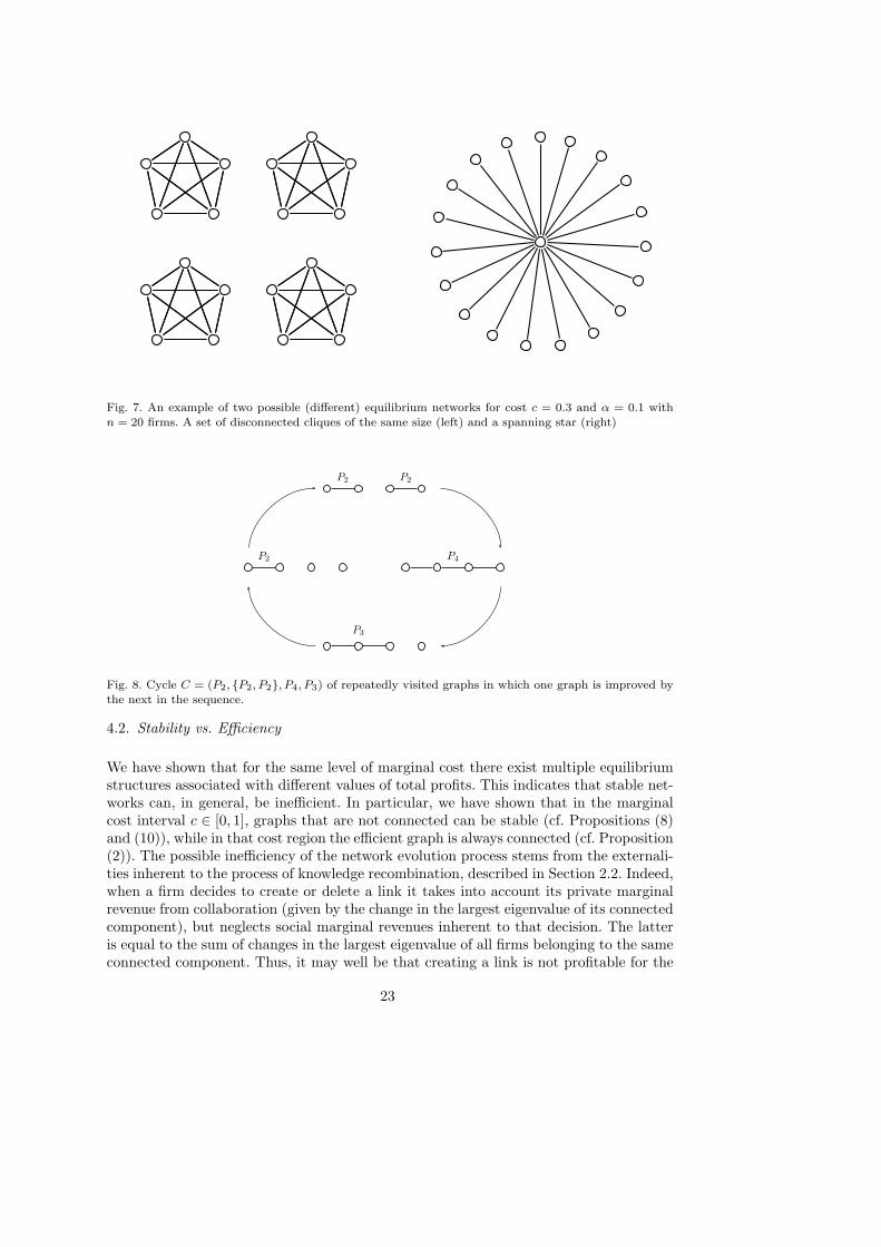
Fig. 7. An example of two possible (different) equilibrium networks for cost c = 0.3 and α = 0.1 with

n = 20 firms. A set of disconnected cliques of the same size (left) and a spanning star (right)

P2

P2 P2

P4

P3

Fig. 8. Cycle C = (P2, {P2, P2}, P4, P3) of repeatedly visited graphs in which one graph is improved bythe next in the sequence.

4.2. Stability vs. Efficiency

We have shown that for the same level of marginal cost there exist multiple equilibriumstructures associated with different values of total profits. This indicates that stable net-works can, in general, be inefficient. In particular, we have shown that in the marginalcost interval c ∈ [0, 1], graphs that are not connected can be stable (cf. Propositions (8)and (10)), while in that cost region the efficient graph is always connected (cf. Proposition(2)). The possible inefficiency of the network evolution process stems from the externali-ties inherent to the process of knowledge recombination, described in Section 2.2. Indeed,when a firm decides to create or delete a link it takes into account its private marginalrevenue from collaboration (given by the change in the largest eigenvalue of its connectedcomponent), but neglects social marginal revenues inherent to that decision. The latteris equal to the sum of changes in the largest eigenvalue of all firms belonging to the sameconnected component. Thus, it may well be that creating a link is not profitable for the

23

individual firm although it would be profitable from the industry point of view.Furthermore, the efficient network may not even belong to the set of equilibria, as it

is shown in the next proposition.

Proposition 12 Consider a network of size n ≥ 2c. For cost c < 1

2 the equilibriumnetwork is not efficient.

This result can be explained in the following way. Proposition (3) states that, when themarginal cost of link formation is less or equal to 1/2, the complete graph is the efficientgraph. However, if the number n of firms in the industry is large enough, the individualmarginal revenue of a collaboration is bounded from above by a value decreasing withn (see the proof of the Proposition (12) in the appendix). In particular, for n ≥ 2

cthe

upper bound is always smaller than the marginal cost c. Therefore the complete graphis not stable 19 .

An exhaustive discussion of efficiency and stability would require the determinationof individual and total profits of firms under all possible network configurations. Bothrequire the computation of the largest eigenvalue. Unfortunately, there is no generalclosed form solution available for any graph. However, one can provide general results forsome special classes of graphs. Based on these findings Table (1) summarizes the resultson efficiency and stability discussed so far and compares them with results for other wellknown classes of graphs in the literature.

Three graphs in the table deserve a special attention. The first is the empty graph,which is never stable nor efficient in the interval [0, 1). The second one is the completegraph, which is efficient in [0, 0.5], but is never stable for c > 0 (see Proposition (5) andProposition (12)). The third graph is the star, which can be stable but is never efficient 20

in [0, 1]. In other words, both the star and the complete graph are never stable and efficientat the same time. This is a first important difference with respect to the literature, e.g.the models in Jackson and Wolinsky (1996) and Bala and Goyal (2000), where, at least inan interval of the parameters considered, the star (or, respectively, the complete graph)can be efficient and stable. In our model the tension between efficiency and stabilityis more pronounced. We were not able to find any efficient graph which is also stable,except from the trivial case of c = 0 in which, due the absence of collaboration cost, thecomplete graph is both stable and efficient.

Moreover, it is interesting to review the properties of the other graphs listed in thetable and their mutual relations. A k-regular graph, i.e. a graph in which all nodes havethe same degree, yields a revenue proportional to the degree of the nodes, regardlessof the size of the graph. This means that when the degree is small the performance interms of aggregate profits of this graph is rather poor. However, the complete graph isa particular case of regular graph in which all nodes have degree n − 1. In this case, theregular graph can be efficient.

The set of cliques of the same size, is stable for particular values of their size d,depending on the level of costs. It can also be efficient, in the particular case of one

19Another (degenerate) region of the parameter space in which the network dynamics leads to inefficient

equilibrium outcomes is the one in which marginal cost is in the open interval (2 −√

2, 1

2

(√5 − 1

)=

(0.586, 0.618). In that case (cf. Proposition (11)), for any number of firms in the industry the dynamics

gets stuck into a cycle of networks, none of which is efficient.20One can show that for c < n

n−1+√

n−1∼ 1 for n → ∞, Kn has a higher performance than K1,n−1.

E.g. for n = 100 we get c < 0.918.

24

set containing all firms, i.e. the complete graph. In this case however, it is never stable,as noted above. The set of identical cliques is also a particular case of k-regular graph,because the nodes in each clique have the same degree. In a path, the degree of the nodesis 2, except from the two nodes at the beginning and at the end of the path. In this sense,the graph is similar to a 2-regular graph. Indeed its eigenvalue is a little smaller thanthe one of 2-regular graph. When the network evolves starting from an empty graph,the first connected graph that is formed is indeed a path of length 2, possibly followedby a path of length 3 (see the proof of Lemma (3) in the appendix). In such transition,the largest eigenvalue of the component jumps from 0 to 1 and then to 2 cos

(π4

)> 1.

Instead, when the graph is almost complete, the addition of a new link yields a negligibleincrease in the eigenvalue. Notice that the path of length 3 is also a star with one huband two peripheral nodes.

A cycle is a closed path and it is in particular a 2-regular graph. In a cycle there isonly one walk, which yields a revenue independent of the number of participating firms.In particular, because of this in our model the path is never an efficient graph. As wealready noticed in Section 2.3, this is a consequence of the payoff function which differsin this respect from the one used in other models in the literature (e.g. Bala and Goyal,2000).

We also list in the table the bipartite graph because of its relation to the notion ofstructural holes (cf. Burt, 1992). In a bipartite graph, nodes can be grouped in twoseparate classes so that links connect only nodes of one class to nodes of the other class.Consider for example a network consisting of few hubs, disconnected among them, and ofmany peripheral nodes, connected only to one or more hubs. The hubs fill the structuralholes among the the peripheral nodes. This network is also a bipartite graph, since thehubs and the peripheral nodes form two separate classes of nodes. Notice that the staris a particular case of a bipartite graph. In our model, the bipartite graph is not efficientnor stable.

Finally, concerning the largest eigenvalue of Fn,d an exact solution (see Bell, 1991) isgiven by the largest root of the cubic polynomial x3−(d−2)x2−(n−1)x+(d−2)(n−d).From this exact solution, one can show that for a fixed value of d, limn→∞ ∆λPF = 0and thus it is always profitable to remove a link if n is large (however large the severancecost or small the marginal cost may be).

4.3. Topological Properties of Stable Networks

The empirical research on R&D partnerships has investigated in depth the topologicalpatterns of networks of knowledge exchange. From this literature (see e.g. Ahuja, 2000;Fleming et al., 2007; Hanaki et al., 2007; Powell et al., 2005), three features emerge asrobust stylized facts: (i) R&D networks are sparse, that is the number of actual links ismuch less than the number of possible links. (ii) Networks are highly clustered, whereclusters consist of highly interconnected firms, but different clusters are only sparselyconnected. (iii) The distribution of links over the firms is characterized by high dispersion,with few firms being connected to many others.

The analytical study of equilibrium networks in Section 4 has pointed to the existenceof equilibrium networks that match some of the stylized facts mentioned above. Indeed,

25

Graph Class Eigenvalue Total Profits Efficiency Stability

empty graphλPF = 0 Π = 0 c > n c > 1

G = Kn

complete graphλPF = n − 1 Π = (1 − c)n(n − 1) c ≤ 1

2 c = 0G = Kn

k-regular graph λPF = k − 1 Π = n(k − 1)(1 − c)if k = n

see cliquessee Kn

pathλPF = 2 cos

(π

n+1

)

Π = 2 cos(

πn+1

)

− (n − 1)c no noG = Pn

starλPF =

√n − 1 Π = n

√n − 1 − 2(n − 1)c

not in⌈ 2

c⌉ ≤ n ≤ ⌊ 1+c′2(6+c′2)

4c′2⌋

G = K1,n−1 0 < c < 1

cycleλPF = 2 Π = 2n(1 − c) no no

G = Cn

bipartite graphλPF =

√n1n2 Π = (n1 + n2)

√n1n2 − n1n2c no no

G = Kn1,n2

G = Fn,d λPF ≥ d − 1 Π = λPF(Fn,d) − 2c((

n2

)+ (n − d)

) with goodno

approx. a

cliques b

λPF = d − 1 Π = n(d − 1)(1 − c)if l = 1, d = n,

⌈ 1+c(1−c)c

⌉ ≤ d ≤ ⌊ 2−c′(1−c′)c′

⌋G = {K1

d , ...,Kld} see Kn

Table 1. Summary of the largest real eigenvalue, total profits, efficiency and stability for different types of networks.

a ∀c, and for large n, total profits of this graph tends to the one of efficient graph, limn→∞ ǫ = 0b We have l cliques of identical size d.

26

equally sized cliques are characterized by a high clustering, while the spanning star showshigh degree heterogeneity. All these networks belong to the set of possible equilibriastructures in our model.

In this section we define an explicit process of network evolution that is a particularcase of improving path and we analyze by means of computer simulations the structuralproperties of stable networks in our model. In this way we explore the existence ofmore complex stable network structures, beyond those described in the previous section.Furthermore, we investigate whether our model is also able to generate pairwise stablestructures that feature, at the same time, all the stylized facts of R&D networks.

There are several possible processes which would be consistent with the definition ofan improving path. In this work, we investigate a stochastic process in which all pairs offirms have the same probability to be selected to revise their R&D collaboration strategy(cf. Vega-Redondo, 2007, p. 212).

Definition 5 (Myopic Pairwise Dynamics) Let G denote the current graph G(t) attime t. We define the network formation process Γ(G) as follows. At the beginning ofeach period (at times t = 0, T, 2T, ...) a single pair of firms, i and j, is uniformly selectedat random from the set N of firms.

(i) If the link ij does not currently exist, ij /∈ E(G), then it is created whenever neitherfirm is harmed by the creation and at least one of them strictly gains, i.e.

πi(G + ij, c) ≥ πi(G, c) ∧ πj(G + ij, c) ≥ πj(G, c)∧πi(G + ij, c) > πi(G, c) ∨ πj(G + ij, c) > πj(G, c).

(23)

or equivalently

λi(G + ij) − λi(G) ≥ c ∧ λj(G + ij) − λj(G) ≥ c∧λi(G + ij) − λi(G) > c ∨ λj(G + ij) − λj(G) > c.

(24)

(ii) If the link ij is currently in place, ij ∈ E(G), then it is removed whenever at leastone of the firms strictly gains from the change, with link deletion involving theseverance cost v(c) = (1 − α)c, and α ∈ [0, 1]. More formally

πi(G − ij, c, v) > πi(G, c, v) ∨ πj(G − ij, c, v) > πj(G, c, v), (25)

or equivalently:

λi(G) − λi(G − ij) < αc ∨ λj(G) − λj(G − ij) < αc (26)

Note that, in the evolution of the network defined above, the only element of stochasticityis the sequence of the pairs of firms chosen to create or delete links.

We study stable network structures arising from this process in computational experi-ments 21 conducted in a large region of the model’s parameter space. More precisely, wecarried out multiple (50 repetitions for each parameter choice) computer simulations of

21When simulating the network evolution discussed in Section 4 the largest real eigenvalue of the networkhas to be computed many times. Since the largest real eigenvalue of a graph can be computed inpolynomial time (Hong, 1993) our model is well suited for numerical investigations.

27

the network dynamics defined in (5) with a fixed number n of firms in the industry 22

(n = 50), starting each from an empty network Kn. For each simulation we selecteda value for the marginal cost c in the interval [0, 1] and a value for the severance costparameter α in the interval 23 [0, 0.5]. As the number of chosen values were respectively12 for the marginal cost and 5 for the severance cost parameter, the total number of com-puter simulations summed up to 3000. The results of the aforementioned Monte-Carloexperiments are shown in the Figures from (9) to (11).

The plots in Figure (9) show typical equilibrium networks obtained in simulations formarginal cost of link formation equal to 0.15 and different values of the severance costparameter α. Recall that severance cost are equal to v = (1−α)c, and thus are inverselyrelated to the parameter α. As the plots reveal, in this region of the parameter space thedynamics in our model is able to generate equilibrium structures displaying the complexfeatures that characterize empirically observed R&D networks (see e.g. Fleming et al.,2007). In particular, for very high severance costs the equilibrium network contains agiant component with a high degree heterogeneity. On the other hand, as severance costsassociated with link deletion fall down (increasing values of α), we observe a significantincrease in the cliquishness of the network, and a reduction of degree heterogeneity.

The insights coming from the foregoing qualitative study are confirmed by a morequantitative analysis of the topological properties of equilibrium graphs. The plots inFigure (10) display respectively the mean and the variance of the network degree distri-bution as functions of the marginal cost c and severance cost parameter α. The meandegree is inversely related to the sparseness of the graph, while degree variance capturesthe degree heterogeneity. As the plots in the figure make clear, higher cost of R&D col-laboration lead to graphs that are more sparse. On the other hand, degree heterogeneityreaches a peak for values of marginal cost close to 0.1, and then falls down as collab-oration costs increase. In addition, degree heterogeneity increases with severance costs(decreasing α).

The presence of clusters of highly interconnected firms is a key feature of empiricallyobserved R&D networks (cf. stylized fact number (iii)). As the plots in Figure (11) show,this feature is also a characteristic for the equilibrium networks generated by the model.In particular, the average clustering coefficient (Figure (11), top-left) is close to one ina wide region of the explored parameter space (c ∈ (0, 0.5), α > 0). Moreover, it is adecreasing function of severance costs v = (1−α)c. Finally, note that clustering becomeszero for values of costs greater or equal to 0.7. Further information on the topologicalfeatures of R&D clusters can be gathered by looking at the average number of connectedcomponents, at their average size and the concentration of their size (Figure (11), top-right, bottom-left and bottom-right respectively). As the plots in the figure indicate, thenumber of connected components is an increasing function of collaboration costs whilethe average size and its concentration variables are negatively related to collaborationcosts. In addition, as the costs of link severance increase the number of componentsincreases, while component size and its concentration decrease.

22Choosing a different, possibly higher, number of firms would have not altered the results, as only thesize (the number of firms) of the connected components, and not the total size of the system matters forthe dynamics.23Preliminary simulation studies with values of α greater than 0.5 for the severance cost did not revealthe presence of any striking difference in the results.

28

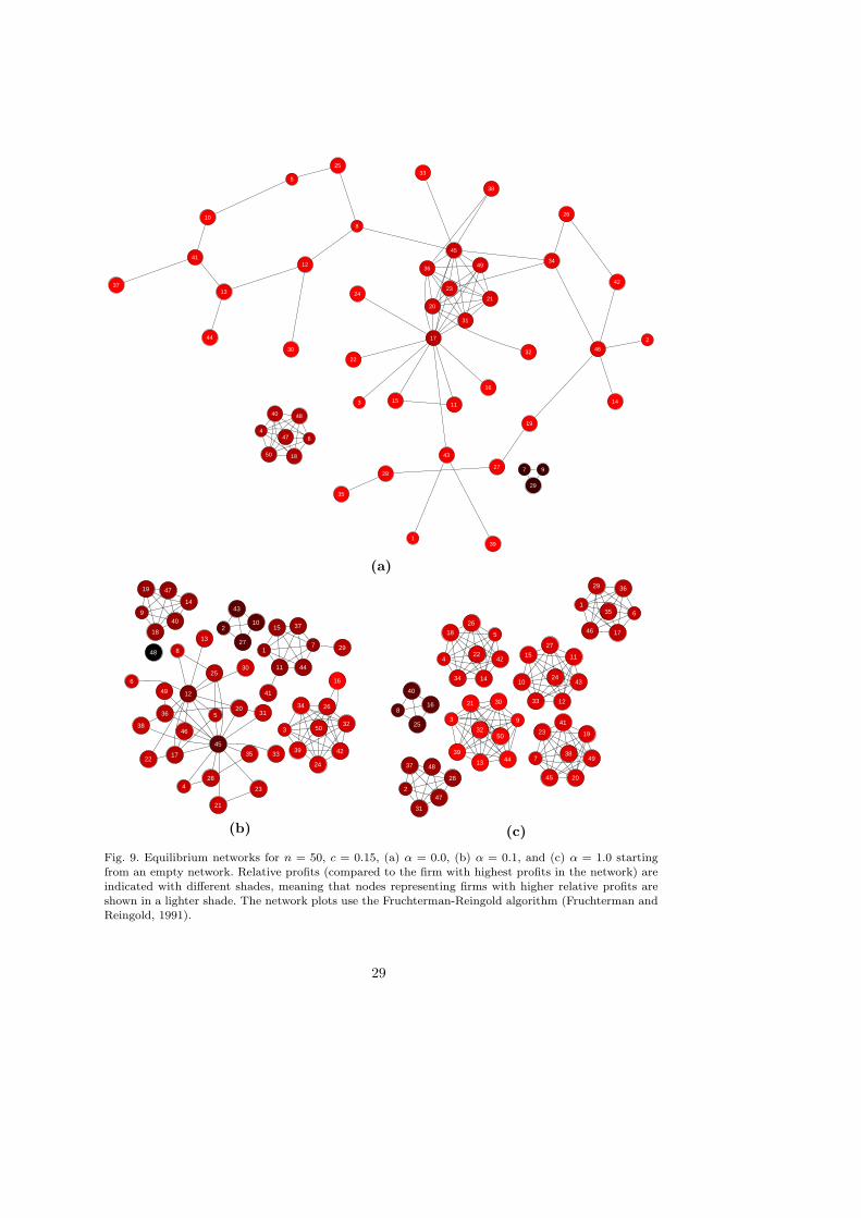
1

43

2

46

3

17

46

18

40

47

48

50

5

10

25

7 9

29

8

12

4541

1115

13

30

44

14

16

2021

22

2324

31

36 49

19

27

32

34

26

42

28

35

33

38

37

39

(a)

17

11

15 37

44

210

27

43

3

24

26

32

34

39 42

50

428

45

5

12

17

256

298

9

14

18

19

40

47

41

13

20

22

30

36

46

16

31

21

23

35 33

38

49

48

(b)

16

17

29

35

36

46

2

28

31

37

47

48

3 9

13

21 30

32

3944

50

4

5

14

18

22

26

34

42

7

19

20

23

38

41

45

49

816

25

4010

11

12

15

24

27

33

43

(c)

Fig. 9. Equilibrium networks for n = 50, c = 0.15, (a) α = 0.0, (b) α = 0.1, and (c) α = 1.0 startingfrom an empty network. Relative profits (compared to the firm with highest profits in the network) are

indicated with different shades, meaning that nodes representing firms with higher relative profits areshown in a lighter shade. The network plots use the Fruchterman-Reingold algorithm (Fruchterman andReingold, 1991).

29

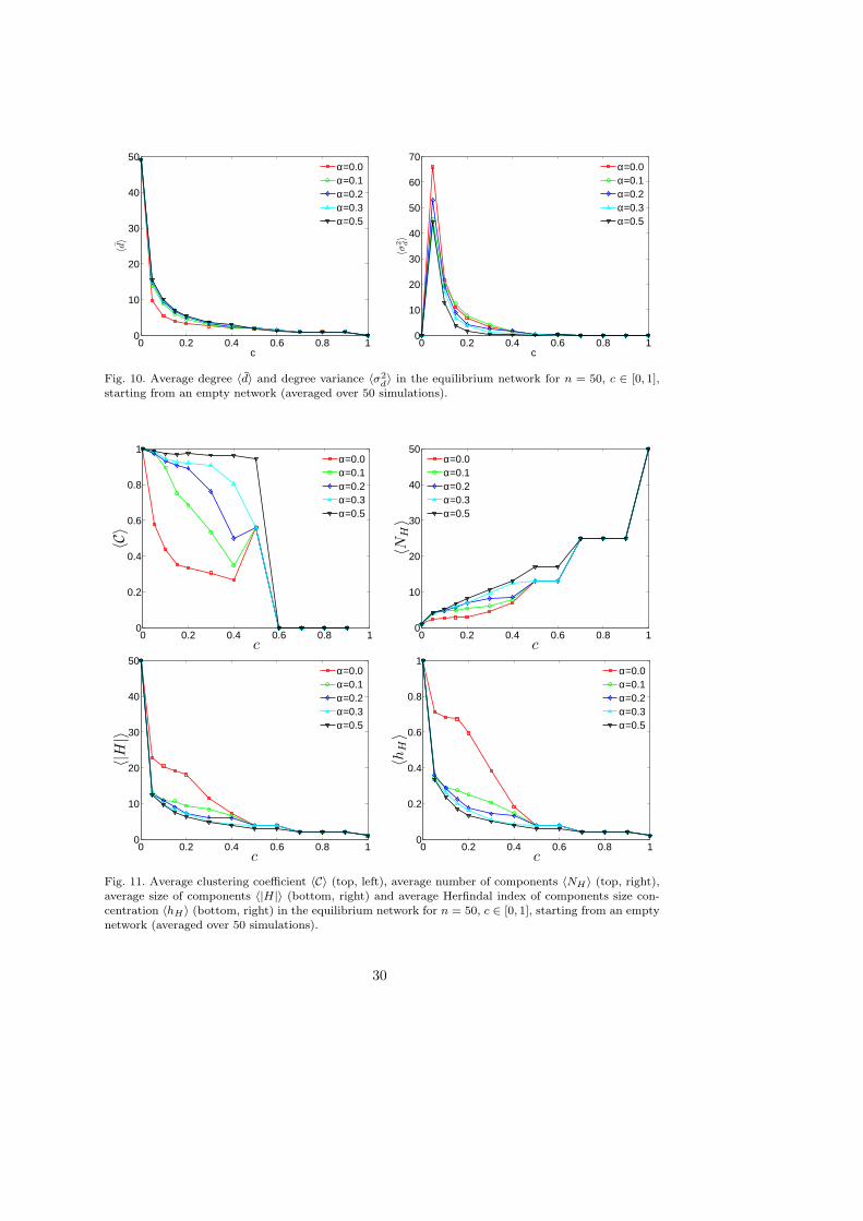
c

0 0.2 0.4 0.6 0.8 10

10

20

30

40

50α=0.0α=0.1α=0.2α=0.3α=0.5

〈d〉

c

0 0.2 0.4 0.6 0.8 10

10

20

30

40

50

60

70α=0.0α=0.1α=0.2α=0.3α=0.5

〈σ2 d〉

Fig. 10. Average degree 〈d〉 and degree variance 〈σ2d〉 in the equilibrium network for n = 50, c ∈ [0, 1],

starting from an empty network (averaged over 50 simulations).

0 0.2 0.4 0.6 0.8 10

0.2

0.4

0.6

0.8

1α=0.0α=0.1α=0.2α=0.3α=0.5

〈C〉

c

0 0.2 0.4 0.6 0.8 10

10

20

30

40

50α=0.0α=0.1α=0.2α=0.3α=0.5

〈NH〉

c

0 0.2 0.4 0.6 0.8 10

10

20

30

40

50α=0.0α=0.1α=0.2α=0.3α=0.5

〈|H|〉

c

0 0.2 0.4 0.6 0.8 10

0.2

0.4

0.6

0.8

1α=0.0α=0.1α=0.2α=0.3α=0.5

〈hH〉

c

Fig. 11. Average clustering coefficient 〈C〉 (top, left), average number of components 〈NH〉 (top, right),average size of components 〈|H|〉 (bottom, right) and average Herfindal index of components size con-

centration 〈hH〉 (bottom, right) in the equilibrium network for n = 50, c ∈ [0, 1], starting from an emptynetwork (averaged over 50 simulations).

30

Joining together the foregoing results we can conclude that sparse equilibrium net-works organized in clusters of highly interconnected firms are a distinctive feature of thenetwork dynamics in our model. Moreover, low values of R&D collaboration costs andhigh values of the costs of link severance lead to equilibrium structures characterizedby a small number of large components, with a highly dispersed degree distribution. Ascollaboration costs increase and as link severance costs decrease, we observe that equilib-rium networks tend to be more and more organized in size homogeneous cliques havingonly few connections among them.

5. Conclusions

In this paper, we have investigated the efficiency and the evolution of networks of knowl-edge exchange across firms. We developed a model in which firms recombine their knowl-edge stock with the stocks of knowledge of other firms in the industry, in order to in-troduce innovations in the market. Since each collaboration is costly for firms they facea trade-off between the benefits of new collaborations (in terms of an increase in theexpected number of innovations per period) and the costs associated with them. Further-more, we showed that under mild conditions on the horizon over which the performanceof R&D collaborations is evaluated, the benefit the firm receives from the network de-pends on the growth rate of all walks existing across firms in their connected component.To this end, our model can be seen as extending other popular models in the networkformation literature (cf. the “connections” model in Jackson and Wolinsky, 1996, andthe linear “two-way flow” model without decay in Bala and Goyal, 2000).

Within the foregoing framework, we characterized the topology of the efficient graphfor any level of the marginal cost of collaboration. We showed that, when the marginalcost of maintaining collaborations is low, the efficient network is the complete graph.Thus, when collaboration costs are low, a network of densely connected firms maximizestotal profits in the industry. On the other hand, as the marginal cost of collaborationincreases it is better for the industry network to display the presence of structural holes.In particular, for intermediate costs of collaboration the efficient graph belongs to theclass of nested split graphs, characterized by the presence of a hub linking a clique to a setof disconnected firms. Furthermore, we showed that nested split graphs are characterizedby significant cross-firm profit inequality, increasing both in collaboration costs and sizeof the industry. Finally, we showed that for very large costs of collaboration the emptygraph is efficient.

We then studied the existence of equilibrium graphs in the model, and the relation be-tween equilibrium and efficiency. For this purpose, we employed the notion of “improvingpath” (cf. Jackson and Watts, 2002), and we assumed that the deletion of existing connec-tions involves a severance cost. In line with the concept of improving path, we identifiedregions of collaboration and severance costs in which there exist either pairwise stablegraphs or a closed cycles of networks. As far as pairwise stable networks are concerned,we showed that different network structures are stable for the same level of costs. Inparticular, we identified regions of the collaboration and severance costs in which (i) thespanning star (i.e. the star encompassing all firms in the network), and (ii) the class ofsize-homogeneous disconnected cliques are stable. In turn, the source of multiplicity ofequilibria lies in (i) the strong path dependency involved in partner selection decisions,

31

(ii) in the presence of external effects affecting marginal revenue of collaborations forfirms belonging to the same connected component and (iii) the inertia arising from thepresence of a severance cost associated with link deletion. The presence of multiple sta-ble structures for the same level of collaboration costs implies that, in general, efficientstructures are not attained in our model. Furthermore, we identified a region of the sizeof the industry and of costs in which the efficient graph is never attained.

Finally, we investigated the topological characteristics of pairwise stable graphs in ourmodel, to see whether they are able to replicate the stylized facts on empirically observedR&D networks. To this end, we studied via computer simulations the properties of equi-libria generated under a two-sided myopic pairwise dynamics (cf. Vega-Redondo, 2007, p.212). The results of our simulations show the existence of a region of low marginal costsof collaboration and high costs of link deletion in which the aforementioned dynamics isable to select pairwise stable structures matching the stylized facts on R&D networks.

The present work could be extended at least in three ways. First, the model couldbe extended to account for industry demand, for example like in Goyal and Moraga-Gonzalez (2001). In this way, one could then study how the efficiency and dynamics ofnetwork structure may change when firms operate in markets that are interdependent.Second, one could investigate whether the foregoing results about the properties of stablenetworks are robust to different link updating algorithms. For example, one could studythe effect on the network dynamics of introducing firms pursuing different strategies, forinstance of the kind explored in Bala and Goyal (2000). Similarly, one could depart fromthe strong assumptions we made on the knowledge firms have about the network. Inthis respect, one could study instead the efficiency and emergence of network structureswhen firms follow more simple rules of behavior, for example of the kind suggested in theempirical work by Powell et al. (2005). Third, in the present model we assumed that theknowledge bases of firms in the industry were sufficiently homogeneous to be transferredacross firms. However, the process of knowledge transfer across firms is likely to be shapedby its degree of tacitness, as well as by the existing technological complementaritiesacross sectors and firms’ knowledge bases. A further analysis of R&D network dynamicsand efficiency should therefore embed all the foregoing ingredients related to industrytechnology, and try to investigate how they may affect the revenues and costs of theprocess of knowledge recombination.

Acknowledgements

Thanks to Hans Haller, Koen Frenken, Luigi Marengo, Giorgio Fagiolo, Paolo Saviotti,Nicolas Carayol, Patrick Groeber, Hans Gersbach and Douglas White for their invaluableadvice and support. Moreover we would like to thank participants at the 5th Interna-tional EMAEE Conference on Innovation in Manchester, 2007, participants at the 12thInternational Conference of the Schumpeter Society in Rio de Janeiro, 2008 and partici-pants at the 14th International Conference on Computing in Economics and Finance inParis, 2008 for their comments. All usual disclaimers apply.

32

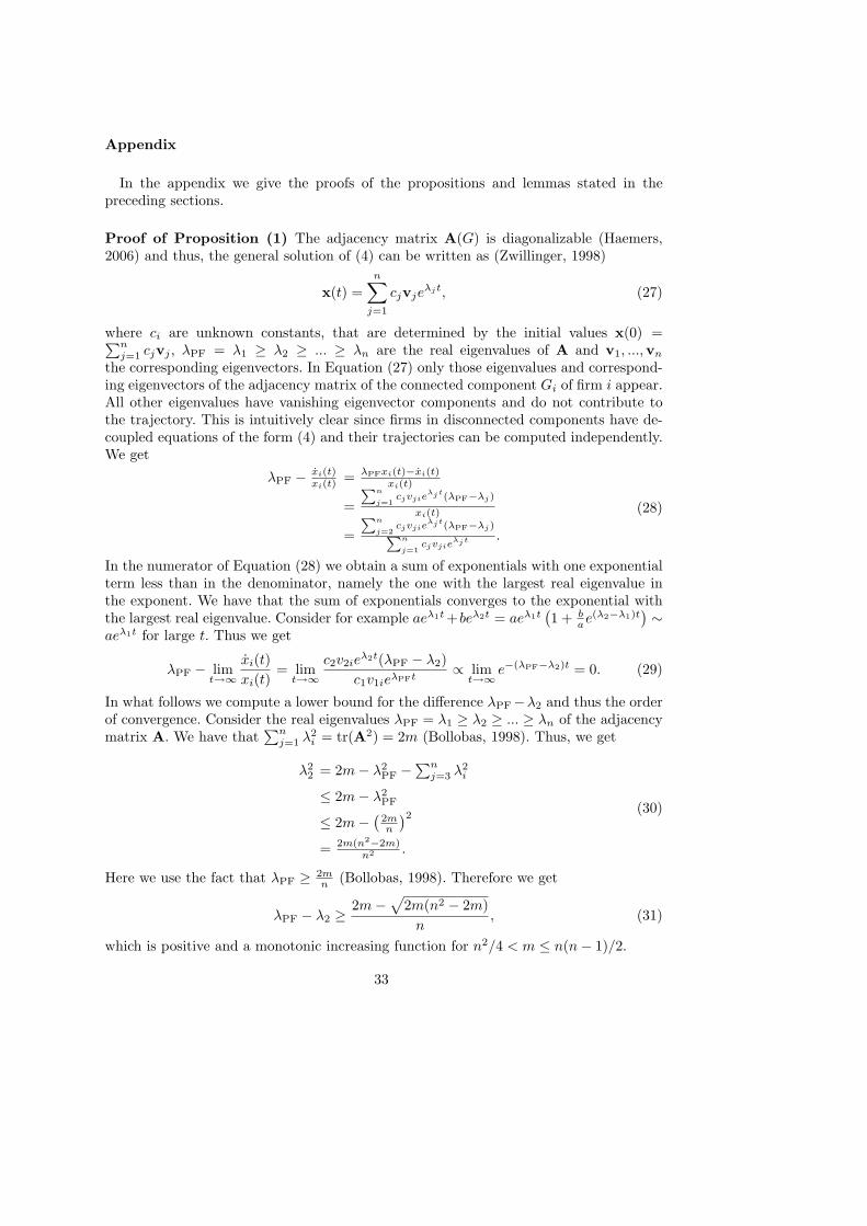
Appendix

In the appendix we give the proofs of the propositions and lemmas stated in thepreceding sections.

Proof of Proposition (1) The adjacency matrix A(G) is diagonalizable (Haemers,2006) and thus, the general solution of (4) can be written as (Zwillinger, 1998)

x(t) =

n∑

j=1

cjvjeλjt, (27)

where ci are unknown constants, that are determined by the initial values x(0) =∑n

j=1 cjvj , λPF = λ1 ≥ λ2 ≥ ... ≥ λn are the real eigenvalues of A and v1, ...,vn

the corresponding eigenvectors. In Equation (27) only those eigenvalues and correspond-ing eigenvectors of the adjacency matrix of the connected component Gi of firm i appear.All other eigenvalues have vanishing eigenvector components and do not contribute tothe trajectory. This is intuitively clear since firms in disconnected components have de-coupled equations of the form (4) and their trajectories can be computed independently.We get

λPF − xi(t)xi(t)

= λPFxi(t)−xi(t)xi(t)

=

∑n

j=1cjvjie

λjt(λPF−λj)

xi(t)

=

∑n

j=2cjvjie

λjt(λPF−λj)∑

n

j=1cjvjie

λjt .

(28)

In the numerator of Equation (28) we obtain a sum of exponentials with one exponentialterm less than in the denominator, namely the one with the largest real eigenvalue inthe exponent. We have that the sum of exponentials converges to the exponential withthe largest real eigenvalue. Consider for example aeλ1t +beλ2t = aeλ1t

(1 + b

ae(λ2−λ1)t

)∼

aeλ1t for large t. Thus we get

λPF − limt→∞

xi(t)

xi(t)= lim

t→∞c2v2ie

λ2t(λPF − λ2)

c1v1ieλPFt∝ lim

t→∞e−(λPF−λ2)t = 0. (29)

In what follows we compute a lower bound for the difference λPF−λ2 and thus the orderof convergence. Consider the real eigenvalues λPF = λ1 ≥ λ2 ≥ ... ≥ λn of the adjacencymatrix A. We have that

∑nj=1 λ2

i = tr(A2) = 2m (Bollobas, 1998). Thus, we get

λ22 = 2m − λ2

PF − ∑nj=3 λ2

i

≤ 2m − λ2PF

≤ 2m −(

2mn

)2

= 2m(n2−2m)n2 .

(30)

Here we use the fact that λPF ≥ 2mn

(Bollobas, 1998). Therefore we get

λPF − λ2 ≥ 2m −√

2m(n2 − 2m)

n, (31)

which is positive and a monotonic increasing function for n2/4 < m ≤ n(n − 1)/2.

33

Proof of Corollary (1) The proof follows directly from an application of the followinglemma.Lemma 4 Consider a continuous function f : [0,∞) → R that converges to a finitevalue λ, i.e. limt→∞ f(t) = λ < ∞. Then

limT→∞

1

T

∫ T

0

f(t)dt = λ. (32)

Proof of Lemma (4) Denote F (T ) = 1T

∫ T

0f(t)dt. We can write

F (T ) =1

T

∫ τ ′

0

f(t)dt

︸ ︷︷ ︸

≤cτ ′

+1

T

∫ T

τ ′

f(t)dt. (33)

The first integral in the above expression is finite since any continuous function on thecompact set [0, τ ′] has a maximum denoted by c. Since f(t) converges to λ, for any ǫ′ wecan find a τ ′(ǫ′) such that for all t ≥ τ ′ we have |f(t) − λ| < ǫ′. Thus we get

|F (T ) − λ| =∣∣∣

1T

(∫ τ ′

0f(t)dt +

∫ T

τ ′f(t)dt − λT

)∣∣∣

≤ 1T

(

|c|τ ′ +∣∣∣

∫ T

τ ′f(t)dt − λT

∣∣∣

)

≤ 1T

(

|c|τ ′ +∫ T

τ ′|f(t) − λ|dt + (T − τ ′ − T )λ

)

≤ 1T

(|c|τ ′ + ǫ′(T − τ ′) − τ ′λ)

= (|c|−λ)τ ′

T+ T−τ ′

Tǫ′

≤ |c|τ ′

T+ ǫ′.

(34)

We define

ǫ = |c|τ ′

T+ ǫ′

τ = |c|τ ′

ǫ−ǫ′.

(35)

Since ∂ǫ∂T

= − |c|τ ′

T 2 < 0 we have that |F (T )− λ| < ǫ for T > τ . For any ǫ > 0 we can findan ǫ′ < ǫ (e.g. ǫ′ = ǫ/2) and the corresponding τ ′(ǫ′) from which we compute τ(ǫ) suchthat |F (T ) − λ| < ǫ for all T > τ(ǫ). This means that limT→∞ F (T ) = λ.

Proof of Lemma (2) Since G1 and G2 are connected, we have that m1 ≥ n1 − 1 andm2 ≥ n2 − 1 (West, 2001). We now consider different cases for the number of edges inthe components.

(i) m1 ≥ n1 and m2 ≥ n2: Assume that the largest eigenvalue of G1 is λPF(G1) ≥λPF(G2). Let G′ be the graph obtained as follows: for each node in G2 we rewire oneincident edge to a node in G1. In this way, all nodes in G2 are connected to G1. Thenumber of rewired edges is n2 (and there are at least that many edges since m2 ≥ n2

by assumption). There exists a relationship between the largest real eigenvalue of agraph and those of its subgraphs (Cvetkovic et al., 1995): if H is a subgraph of G,

34

H ⊆ G, then λPF(H) ≤ λPF(G). Therefore, λPF(G′) ≥ λPF(G1) ≥ λPF(G2). Totalprofits of G′ are

Π(G′) = (n1 + n2)λPF(G′) − 2(m1 + m2)c

≥ n1λPF(G1) + n2λPF(G2) − 2(m1 + m2)c

= Π(G1) + Π(G2).

(36)

(ii) m1 ≥ n1 and m2 = n2 − 1: If m2 = n2 − 1 then the largest real eigenvalue of G2 isat most the one of the star K1,n2−1 with λPF(G2) ≤

√n2 − 1 (Hong, 1993).

We construct the graph G by connecting all nodes of K1,n2−1 to a single node inG1 and including the remaining isolated node by adding one more edge. The graphG has an eigenvalue λPF(G) ≥ λPF(K1,n1+n2−1) =

√n1 + n2 − 1. Otherwise, the

edges in G are redistributed to form a star K1,n1+n2−1 and the remaining edges areattached at random. Since λPF is an increasing function of the number of edges inthe graph the inequality follows. We obtain

Π(G) = (n1 + n2)λPF(G) − 2(m + 1)c

Π(G1) + Π(G2) = n1λPF(G1) + n2

√n2 − 1 − 2 (m1 + (n2 − 1))

︸ ︷︷ ︸

m

c (37)

Thus, we get

Π(G) − (Π(G1) + Π(G2)) = Π(G) − (Π(G1) + Π(K1,n2−1))

= n1 (λPF(G) − λPF(G1))︸ ︷︷ ︸

≥0

+n2(λPF(G) −√n2 − 1) − 2c

≥ n2(λPF(G) −√n2 − 1) − 2c.

(38)

With λPF(G) ≥ √n1 + n2 − 1 ≥ √

n2 + 1 if n1 ≥ 2 (by assumption). If the lastinequality above is large than 0, we have that

√n2 + 1 −

√n2 − 1 ≥ 2c

n2. (39)

If 0 ≤ c ≤ 1, this inequality is true if n2 ≥ 2 (by assumption).(iii) m1 = n1 − 1 and m2 = n2 − 1: If m1 = n1 − 1 and m2 = n2 − 1, then both

components are stars, K1,n1−1 and K1,n2−1 with eigenvalues√

n1 − 1 and√

n2 − 1.Construct the graph G by connecting n2−1 nodes from K1,n2−1 to the central nodein K1,n1−1. Then attach an edge to the remaining isolated node to obtain a starG = K1,n1+n2−1.

Π(G) = Π(K1,n1+n2−1) = (n1 + n2)√

n1 + n2 − 1 − 2c(n1 + n2 − 1) (40)

For the difference we get

35

Π(G) − (Π(K1,n2−1) + Π(K1,n2−1)) = n1(√

n1 + n2 − 1 −√n1 − 1)

+n2(√

n1 + n2 − 1 −√n2 − 1) − 2c

≥ (n1 + n2)(√

n1 + n2 − 1 −√n1 − 1).

(41)W.l.o.g. we have assumed that n1 ≥ n2. The expression above is larger or equalthan 0 if

(n1 + n2)︸ ︷︷ ︸

≥n1+2

(√

n1 + n2 − 1 −√

n1 − 1︸ ︷︷ ︸

≥√

n1+1−√

n1−1

) ≥ 2 ≥ 2c, (42)

with n2 ≥ 2. We get√

n1 + 1 −√

n1 − 1 ≥ 2

n1 + 2, (43)

and the last inequality holds for n1 ≥ 2.(iv) n1 ≥ 2 and n2 = 1: We have one isolated node and a connected graph G1. Total

profits are Π(G) = n1λPF(G1)−2m1c. Denote the graph G′ obtained by connectingthe isolated node to G1. Then

Π(G′) = (n1 + 1)λPF(G′) − 2(m1 + 1)c

≥ Π(G) + (λPF(G′) − 2c),(44)

We now consider three more cases:(1) If n1 ≥ 4, then m1 ≥ n1 − 1 (since G1 is connected by assumption). We can

construct a star K1,n1−1 plus additional edges from G1 and connect the isolatednode to it. Denote the resulting graph G′. Then, λPF(G′) ≥ λPF(K1,n1

) =√

n1 ≥ 2.Thus, Π(G′) − Π(G) ≥ 0 if λPF(G′) ≥ 2 ≥ 2c for c ∈ [0, 1].

(2) If n1 = 3, then G1 is either a path P3 of length 3 or a cycle C3 containing 3nodes. We connect the isolated node to G1. In the case of G1 = P3 we get

Π(G′) − Π(G) = 4√

3 − 6c︸ ︷︷ ︸

Π(G′)

− (3√

2 − 4c)︸ ︷︷ ︸

Π(G)

= 2.69 − 2c > 0,

(45)

where the last inequality follows from c ∈ [0, 1]. In the case of G1 = C3 we obtain

Π(G′) − Π(G) = 42.17 − 8c︸ ︷︷ ︸

Π(G′)

− (32 − 6c)︸ ︷︷ ︸

Π(G)

= 2.68 − 2c > 0

, (46)

again, using c ∈ [0, 1].(3) For n1 = 2 we connect the isolated node to G1 = P2 and again denote the

resulting connected graph G′. We have that

Π(G′) − Π(G) = 3√

2 − 4c︸ ︷︷ ︸

Π(G′)

− (21 − 2c)︸ ︷︷ ︸

Π(G)

= 2.24 − 2c > 0

, (47)

with c ∈ [0, 1].

36

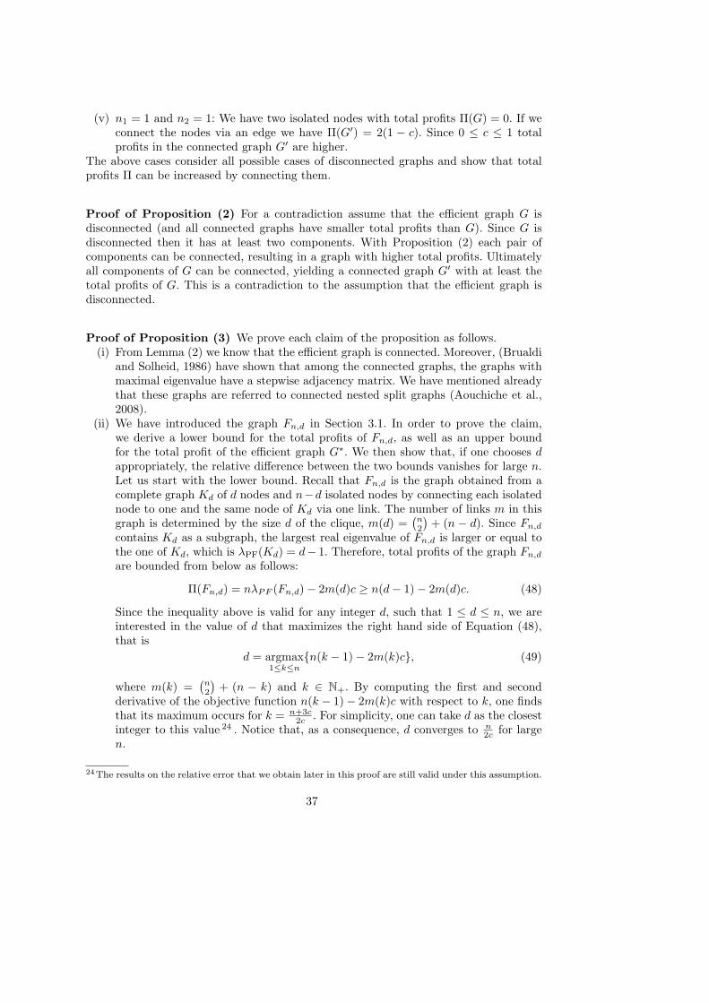
(v) n1 = 1 and n2 = 1: We have two isolated nodes with total profits Π(G) = 0. If weconnect the nodes via an edge we have Π(G′) = 2(1 − c). Since 0 ≤ c ≤ 1 totalprofits in the connected graph G′ are higher.

The above cases consider all possible cases of disconnected graphs and show that totalprofits Π can be increased by connecting them.

Proof of Proposition (2) For a contradiction assume that the efficient graph G isdisconnected (and all connected graphs have smaller total profits than G). Since G isdisconnected then it has at least two components. With Proposition (2) each pair ofcomponents can be connected, resulting in a graph with higher total profits. Ultimatelyall components of G can be connected, yielding a connected graph G′ with at least thetotal profits of G. This is a contradiction to the assumption that the efficient graph isdisconnected.

Proof of Proposition (3) We prove each claim of the proposition as follows.(i) From Lemma (2) we know that the efficient graph is connected. Moreover, (Brualdi

and Solheid, 1986) have shown that among the connected graphs, the graphs withmaximal eigenvalue have a stepwise adjacency matrix. We have mentioned alreadythat these graphs are referred to connected nested split graphs (Aouchiche et al.,2008).

(ii) We have introduced the graph Fn,d in Section 3.1. In order to prove the claim,we derive a lower bound for the total profits of Fn,d, as well as an upper boundfor the total profit of the efficient graph G∗. We then show that, if one chooses dappropriately, the relative difference between the two bounds vanishes for large n.Let us start with the lower bound. Recall that Fn,d is the graph obtained from acomplete graph Kd of d nodes and n−d isolated nodes by connecting each isolatednode to one and the same node of Kd via one link. The number of links m in thisgraph is determined by the size d of the clique, m(d) =

(n2

)+ (n − d). Since Fn,d

contains Kd as a subgraph, the largest real eigenvalue of Fn,d is larger or equal tothe one of Kd, which is λPF(Kd) = d− 1. Therefore, total profits of the graph Fn,d

are bounded from below as follows:

Π(Fn,d) = nλPF (Fn,d) − 2m(d)c ≥ n(d − 1) − 2m(d)c. (48)

Since the inequality above is valid for any integer d, such that 1 ≤ d ≤ n, we areinterested in the value of d that maximizes the right hand side of Equation (48),that is

d = argmax1≤k≤n

{n(k − 1) − 2m(k)c}, (49)

where m(k) =(n2

)+ (n − k) and k ∈ N+. By computing the first and second

derivative of the objective function n(k − 1) − 2m(k)c with respect to k, one findsthat its maximum occurs for k = n+3c

2c. For simplicity, one can take d as the closest

integer to this value 24 . Notice that, as a consequence, d converges to n2c

for largen.

24The results on the relative error that we obtain later in this proof are still valid under this assumption.

37

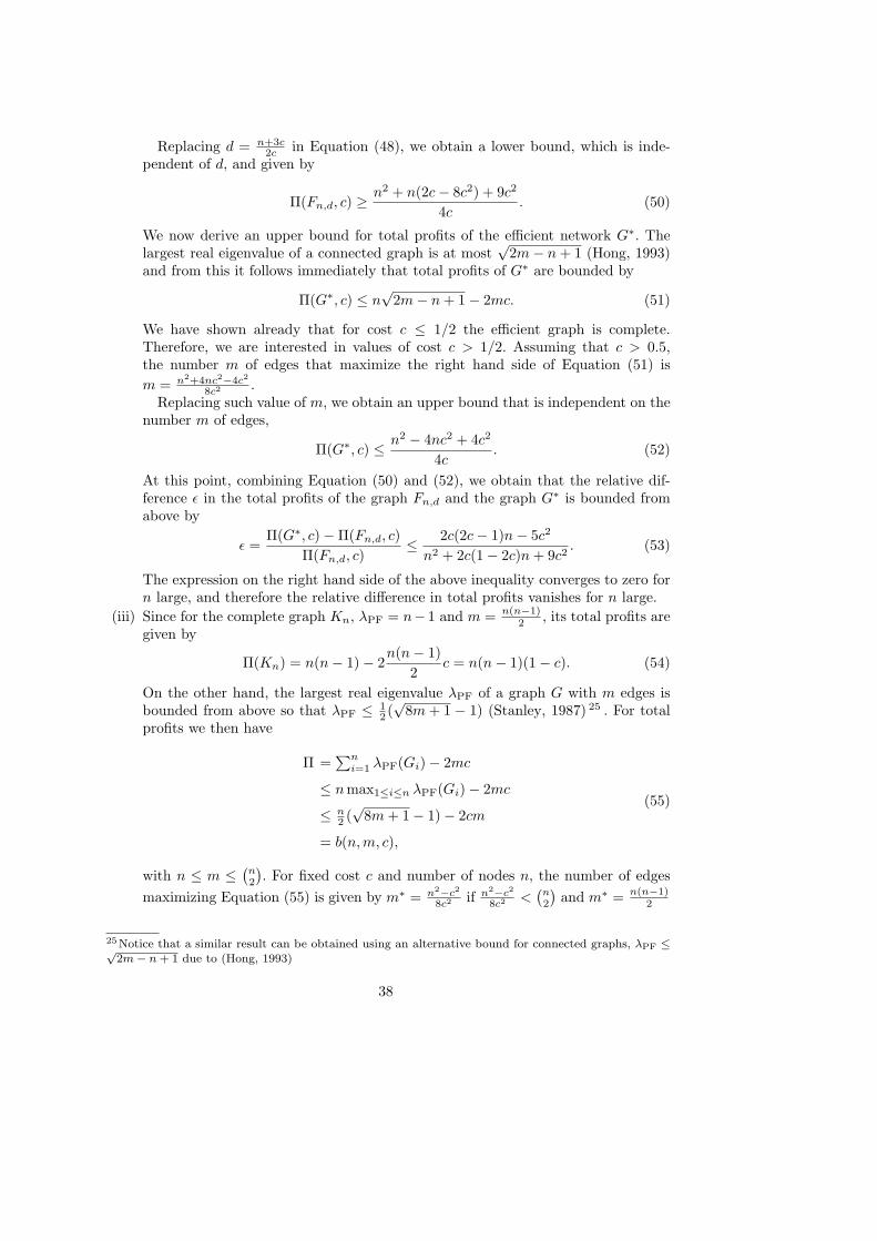
Replacing d = n+3c2c

in Equation (48), we obtain a lower bound, which is inde-pendent of d, and given by

Π(Fn,d, c) ≥n2 + n(2c − 8c2) + 9c2

4c. (50)

We now derive an upper bound for total profits of the efficient network G∗. Thelargest real eigenvalue of a connected graph is at most

√2m − n + 1 (Hong, 1993)

and from this it follows immediately that total profits of G∗ are bounded by

Π(G∗, c) ≤ n√

2m − n + 1 − 2mc. (51)

We have shown already that for cost c ≤ 1/2 the efficient graph is complete.Therefore, we are interested in values of cost c > 1/2. Assuming that c > 0.5,the number m of edges that maximize the right hand side of Equation (51) is

m = n2+4nc2−4c2

8c2 .Replacing such value of m, we obtain an upper bound that is independent on the

number m of edges,

Π(G∗, c) ≤ n2 − 4nc2 + 4c2

4c. (52)

At this point, combining Equation (50) and (52), we obtain that the relative dif-ference ǫ in the total profits of the graph Fn,d and the graph G∗ is bounded fromabove by

ǫ =Π(G∗, c) − Π(Fn,d, c)

Π(Fn,d, c)≤ 2c(2c − 1)n − 5c2

n2 + 2c(1 − 2c)n + 9c2. (53)

The expression on the right hand side of the above inequality converges to zero forn large, and therefore the relative difference in total profits vanishes for n large.

(iii) Since for the complete graph Kn, λPF = n− 1 and m = n(n−1)2 , its total profits are

given by

Π(Kn) = n(n − 1) − 2n(n − 1)

2c = n(n − 1)(1 − c). (54)

On the other hand, the largest real eigenvalue λPF of a graph G with m edges isbounded from above so that λPF ≤ 1

2 (√

8m + 1 − 1) (Stanley, 1987) 25 . For totalprofits we then have

Π =∑n

i=1 λPF(Gi) − 2mc

≤ nmax1≤i≤n λPF(Gi) − 2mc

≤ n2 (√

8m + 1 − 1) − 2cm

= b(n,m, c),

(55)

with n ≤ m ≤(n2

). For fixed cost c and number of nodes n, the number of edges

maximizing Equation (55) is given by m∗ = n2−c2

8c2 if n2−c2

8c2 <(n2

)and m∗ = n(n−1)

2

25Notice that a similar result can be obtained using an alternative bound for connected graphs, λPF ≤√2m − n + 1 due to (Hong, 1993)

38

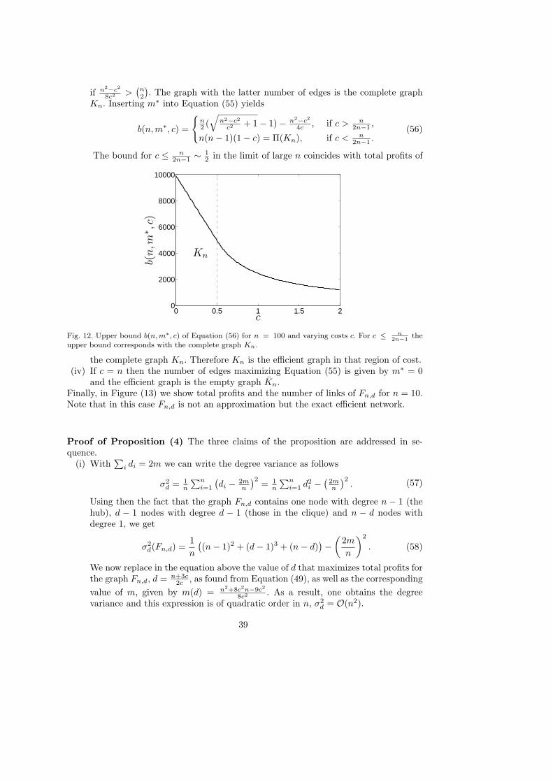
if n2−c2

8c2 >(n2

). The graph with the latter number of edges is the complete graph

Kn. Inserting m∗ into Equation (55) yields

b(n,m∗, c) =

{n2 (

√n2−c2

c2 + 1 − 1) − n2−c2

4c, if c > n

2n−1 ,

n(n − 1)(1 − c) = Π(Kn), if c < n2n−1 .

(56)

The bound for c ≤ n2n−1 ∼ 1

2 in the limit of large n coincides with total profits of

0 0.5 1 1.5 20

2000

4000

6000

8000

10000

b(n,m

∗ ,c)

Kn

c

Fig. 12. Upper bound b(n, m∗, c) of Equation (56) for n = 100 and varying costs c. For c ≤ n2n−1

the

upper bound corresponds with the complete graph Kn.

the complete graph Kn. Therefore Kn is the efficient graph in that region of cost.(iv) If c = n then the number of edges maximizing Equation (55) is given by m∗ = 0

and the efficient graph is the empty graph Kn.Finally, in Figure (13) we show total profits and the number of links of Fn,d for n = 10.Note that in this case Fn,d is not an approximation but the exact efficient network.

Proof of Proposition (4) The three claims of the proposition are addressed in se-quence.

(i) With∑

i di = 2m we can write the degree variance as follows

σ2d = 1

n

∑ni=1

(di − 2m

n

)2= 1

n

∑ni=1 d2

i −(

2mn

)2. (57)

Using then the fact that the graph Fn,d contains one node with degree n − 1 (thehub), d − 1 nodes with degree d − 1 (those in the clique) and n − d nodes withdegree 1, we get

σ2d(Fn,d) =

1

n

((n − 1)2 + (d − 1)3 + (n − d)

)−

(2m

n

)2

. (58)

We now replace in the equation above the value of d that maximizes total profits forthe graph Fn,d, d = n+3c

2c, as found from Equation (49), as well as the corresponding

value of m, given by m(d) = n2+8c2n−9c2

8c2 . As a result, one obtains the degreevariance and this expression is of quadratic order in n, σ2

d = O(n2).

39

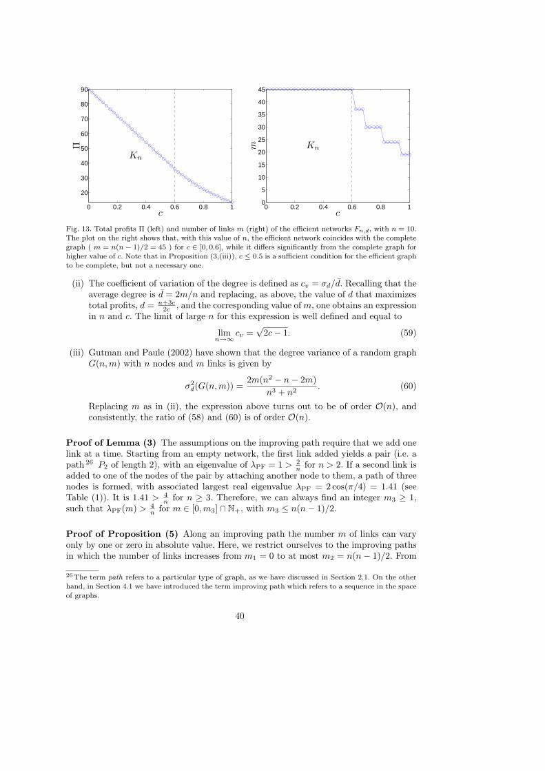
0 0.2 0.4 0.6 0.8 1

20

30

40

50

60

70

80

90

Π

c

Kn

0 0.2 0.4 0.6 0.8 10

5

10

15

20

25

30

35

40

45

m

c

Kn

Fig. 13. Total profits Π (left) and number of links m (right) of the efficient networks Fn,d, with n = 10.

The plot on the right shows that, with this value of n, the efficient network coincides with the completegraph ( m = n(n − 1)/2 = 45 ) for c ∈ [0, 0.6], while it differs significantly from the complete graph forhigher value of c. Note that in Proposition (3,(iii)), c ≤ 0.5 is a sufficient condition for the efficient graphto be complete, but not a necessary one.

(ii) The coefficient of variation of the degree is defined as cv = σd/d. Recalling that theaverage degree is d = 2m/n and replacing, as above, the value of d that maximizestotal profits, d = n+3c

2c, and the corresponding value of m, one obtains an expression

in n and c. The limit of large n for this expression is well defined and equal to

limn→∞

cv =√

2c − 1. (59)

(iii) Gutman and Paule (2002) have shown that the degree variance of a random graphG(n,m) with n nodes and m links is given by

σ2d(G(n,m)) =

2m(n2 − n − 2m)

n3 + n2. (60)

Replacing m as in (ii), the expression above turns out to be of order O(n), andconsistently, the ratio of (58) and (60) is of order O(n).

Proof of Lemma (3) The assumptions on the improving path require that we add onelink at a time. Starting from an empty network, the first link added yields a pair (i.e. apath 26 P2 of length 2), with an eigenvalue of λPF = 1 > 2

nfor n > 2. If a second link is

added to one of the nodes of the pair by attaching another node to them, a path of threenodes is formed, with associated largest real eigenvalue λPF = 2 cos(π/4) = 1.41 (seeTable (1)). It is 1.41 > 4

nfor n ≥ 3. Therefore, we can always find an integer m3 ≥ 1,

such that λPF(m) > 4n

for m ∈ [0,m3] ∩ N+, with m3 ≤ n(n − 1)/2.

Proof of Proposition (5) Along an improving path the number m of links can varyonly by one or zero in absolute value. Here, we restrict ourselves to the improving pathsin which the number of links increases from m1 = 0 to at most m2 = n(n − 1)/2. From

26The term path refers to a particular type of graph, as we have discussed in Section 2.1. On the otherhand, in Section 4.1 we have introduced the term improving path which refers to a sequence in the spaceof graphs.

40

Proposition (1) we know that the largest real eigenvalue is bounded, λPF(m) ≤ n − 1.Taking the average between the extreme values λPF(m1) = 0 and λPF(m2) = n − 1we get an average increase of λPF(m) per additional link of 2

n. This fact is depicted

by the straight line in Figure (5) which has a slope of 2n

and intersects the origin.Moreover, Figure (5) shows an example of an improving path that reaches 50% of thedensity of a complete graph before it arrives at a stable network. Let us now defineym = λPF(m) − 2

nm. ym is just the difference between the largest real eigenvalue of

the improving path and the straight line in Figure (5). Since we have that ym1= 0

and ym2= 0, it obviously holds that the sum of the increments ∆ym = ym − ym−1 in

I = [m1,m2] ∩ N+, have to be zero, that is

m2∑

m=m1+1

∆ym = 0. (61)

However, Lemma 3 ensures that along the improving path, ym starts off positive. There-fore, we can always find an integer m3 ≥ 1, such that (1) ym3

= b > 0 and (2) I = I1∪I2,with I1 = [m1,m3] ∩ N+ and I2 = [m3,m2] ∩ N+. The condition (61) on the incrementsof y implies that

∑

m∈I2

∆ym = −∑

m∈I1

∆ym = −b. (62)

Denoting by 〈∆y〉I2the average increment in the set I2, we have

∑

m∈I2

∆ym = 〈∆y〉I2(m2 − m3). (63)

There must be some increments that are smaller or equal to the average increment.Hence, there must exists a value m∗ such that

∆ym∗ ≤ − b

m2 − m3< 0, (64)

or, equivalently, there exists an m∗ such that

∆λPF(m∗) <2

n. (65)

For any given cost c, we can find an n large enough and an m∗ such that ∆λPF(m∗) < c.This means that the marginal revenue is smaller than the cost, for some value of m∗.This concludes the proof.

Proof of Proposition (6) If costs are zero, c = 0, then the change in eigenvalue equalsthe change in profits. Since (in a connected graph G) each link created strictly increasesλPF (Horn and Johnson, 1990) and accordingly profits, the complete graph Kn is reachedeventually.

Proof of Proposition (7) There exists the following bound on the change in eigenvalueby the removal and creation of a link (Cvetkovic et al., 1995): If the graphs G,G′ differin one edge only then |λPF(G′) − λPF(G)| ≤ 1. A link is created if ∆λPF > c. Thus, nolink is created if c = 1. On the other hand, a link is removed, if ∆λPF < c′. And thus,all links are removed if c′ > 1 and we obtain an empty graph Kn.

41

0 0.2 0.4 0.6 0.8 10

5

10

15

20

25

30

35

40

n

c

min n

max n (α = 1.0)

max n (α = 0.1)

0 0.1 0.2 0.3 0.4 0.510

0

101

102

103

104

num

.st

able

cliq

ue-

size

s

c

α = 1.0α = 0.1

Fig. 14. Upper and lower bounds for the size of the stable cliques (left) and the number of different sizesof stable cliques (right) for α = 1 and α = 0.1.

Proof of Proposition (8) The structure of the proof is as follows. We want to showthat the graph G consisting of k cliques of the same size is stable, that is, no link isremoved or created. For the removal, we can focus on links between nodes in the sameclique, since these are the only links in G. Thus, in Proposition (13) we show that, for anypair of nodes in the same clique, the link is not removed as long as the size n of the clique

is smaller than a given bound br. In particualar, we will show that, br = ⌊ 2−c′(1−c′)c′

⌋.For the creation of links, we can focus on links between nodes in different cliques, since

these are the only new links that can be added to the graph. Thus, in Proposition (14)we show that for any pair of firms belonging to different cliques, a link between them isnot created as long as the size n of the clique is larger than another bound bc, and we

will show that bc = ⌈ 1+c(1−c)c

⌉.It turns out that the bound for the removal, br, is larger than the bound for the

creation, bc, for any value of c ∈ [0, 1], as it is shown in Figure (14). However, since thesize n of the clique has to be an integer, the interval [bc, br] needs to contain at least oneinteger. This can be done constructively. We explored the interval c ∈ [0, 1] with costincrements of 10−3 and we counted the number of integer values that fall within [bc, br].As it is shown in Figure (6), for c < 0.35, there is always at least one integer in betweenthe two bounds, while for c < 0.2, there are always several integers falling in between thetwo bounds.

This is a remarkable finding as it implies that for the values of cost given above, thereexists a multiplicity of equilibria. Indeed, for a given value of cost, the stable graphs areall the configurations with cliques of the same size n, where n varies among the integersincluded in the interval [bc, br].

Propositions (8) and (13), used for this proof, are given below.

Proposition 13 Consider a clique Kn and denote by Kn − ij the graph obtained from

Kn by removing an edge ij. Then λPF(Kn) − λPF(Kn − ij) > c′ if n ≤ ⌊ 2−c′(1−c′)c′

⌋.

Proof of Proposition (13) Denote the matrix obtained from the adjacency matrix Aof Kn − ij, and subtracting the variable λ on the diagonal of A by M = A− λI. M is a

42

block matrix of the form

M =

K BT

B D

, (66)

with submatrices 27

K =

−λ 1 · · · · · · 1

1 −λ...

.... . .

1

1 · · · 1 −λ

(n−2)×(n−2)

, (67)

B =

1 1 1 1 1 1 · · ·1 1 1 1 1 1 · · ·

2×n

, (68)

D =

−λ 0

0 −λ

2×2

. (69)

Since M is a block-matrix (Horn and Johnson, 1990) we can write

det(M) = det(K) det(P). (70)

We have the following lemma.Lemma 5

det

a 1 · · · · · · 1

1 a...

.... . .

...

1

1 · · · · · · 1 a

n×n

= ((n − 1) + a) (a − 1)n−1. (71)

Proof of Lemma (5) The above determinant can be written as det (U − (1 − a)I),where U is a matrix consisting of all ones, uij = 1 i, j = 1, ..., n and I is the identitymatrix. Hence, the eigenvalues of the above matrix are minus 1−a the eigenvalues of U.U has eigenvalues n and 0 with multiplicities 1 and n − 1 respectively (Horn and John-

son, 1990). Therefore, we can write for the determinant (n − (1 − a)) (0 − (1 − a))n−1

=((n − 1) + a) (a − 1)n−1.

Thus, we get for the determinant of K

detK = − ((n − 1) − λ) (1 + λ)n−1. (72)

27The numbers at the bottom right of the matrix indicate the dimension of the matrix.

43

The Schur complement is P = D−BK−1BT . Multiplying the inverse of K with B fromthe left and BT from the right we obtain

BK−1BT = ||K−1||1

1 1

1 1

(73)

where ||K−1||1 is the sum of all elements in the matrix K−1 (the l1 norm of the matrixK−1 (Horn and Johnson, 1990)). By computing K−1K = I one can verify that

K−1 =

n−4−λ(λ−(n−3))(1+λ) − 1

(λ−(n−3))(1+λ) · · ·

− 1(λ−(n−3))(1+λ)

. . .

...

. (74)

And, by summation over the elements in K−1, we obtain ||K−1||1 = n−2(n−3)−λ

. Conse-

quently, the determinant of the Schur complement P is given by

det(P) = (1 + λ)n−3λ(λ2 − (n − 3)λ − 2(n − 2)

). (75)

The largest real eigenvalue of Kn − ij is given by the root of

λ2 − (n − 3)λ − 2(n − 2) = 0. (76)

Thus we get

λPF =1

2

(

n − 3 +√

n2 + 2n − 7)

. (77)

For the change in eigenvalue ∆λPF = λPF(Kn) − λPF(Kn − ij) we obtain

∆λPF =1

2

(

n + 1 −√

n2 + 2n − 7)

, (78)

since λPF(Kn) = n− 1. This is a decreasing function in n. Then for n ∈ N, ∆λPF > c′ if

n ≤ ⌊2 − c′(1 − c′)

c′⌋. (79)

For c′ = 2 −√

2 = 0.586 we have n ≤ 3 and for c′ = 1 we obtain n ≤ 2.

Proposition 14 Denote the graph consisting of two disconnected cliques by G and thegraph obtained from G by connecting the two cliques in G via an edge by G′. Then for

n ≥ ⌈ 1+c(1−c)c2 ⌉ we have λPF(G′) − λPF(G) < c.

Proof of Proposition (14) Denote the adjacency matrix of the graph obtained byconnecting two complete subgraphs Kn and Kn via and edge, see Figure (15), by A.And denote the matrix obtained by subtracting the variable λ on the diagonal of A byM = A − λI. The eigenvalues of A are given by the roots of the determinant of M. Mhas the form of a block matrix with the submatrices K and B. We have

M =

K B

BT K

, (80)

44

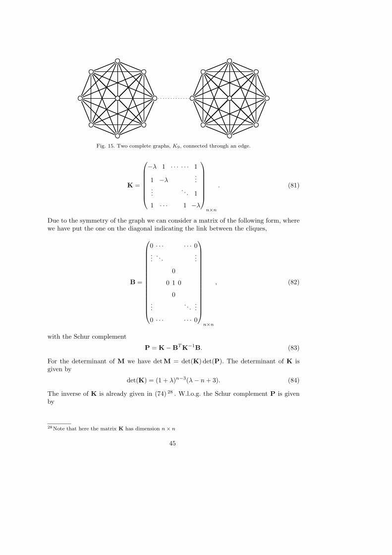
Fig. 15. Two complete graphs, K9, connected through an edge.

K =

−λ 1 · · · · · · 1

1 −λ...

.... . . 1

1 · · · 1 −λ

n×n

. (81)

Due to the symmetry of the graph we can consider a matrix of the following form, wherewe have put the one on the diagonal indicating the link between the cliques,

B =

0 · · · · · · 0...

. . ....

0

0 1 0

0...

. . ....

0 · · · · · · 0

n×n

, (82)

with the Schur complement

P = K − BT K−1B. (83)

For the determinant of M we have detM = det(K) det(P). The determinant of K isgiven by

det(K) = (1 + λ)n−3(λ − n + 3). (84)

The inverse of K is already given in (74) 28 . W.l.o.g. the Schur complement P is givenby

28Note that here the matrix K has dimension n × n

45

P =

−λ 1 · · · · · · 1

1 −λ...

.... . .

−λ 1

1 · · · 1 −λ + λ−(n−2)(λ−(n−1))(1+λ)

. (85)

In the next step we make use of the following lemma.Lemma 6

det

b 1 · · · 1

1 a...

.... . .

a 1

1 · · · 1 a

n×n

= (1 − n + (n − 2)b + ab) (a − 1)n−2. (86)

Proof of Lemma (6) We give a proof by induction. For n = 2 we get

det

b 1

1 a

2×2

= ab − 1 = (b(2 − 2) + ab − (2 − 1))(a − 1)0. (87)

For n = 3 we get

det

b 1 1

1 a 1

1 1 a

3×3

= a2b − 2a + 2 − b = (b + ab − 2)(a − 1). (88)

For the induction step we apply a Laplace expansion of the determinant in (86) intoMinors.

b det

a 1 · · · · · · 1

1 a...

.... . .

a 1

1 · · · 1 a

(n−1)×(n−1)

− (n − 1) det

1 1 · · · · · · 1

1 a...

.... . .

a 1

1 · · · 1 a

(n−1)×(n−1)

(89)

For the first determinant we can use Lemma (5) and for the second the induction hy-pothesis in order to obtain

b ((n − 2) + a) (a − 1)n−2 − (n − 1)(a − 1)n−2. (90)

46

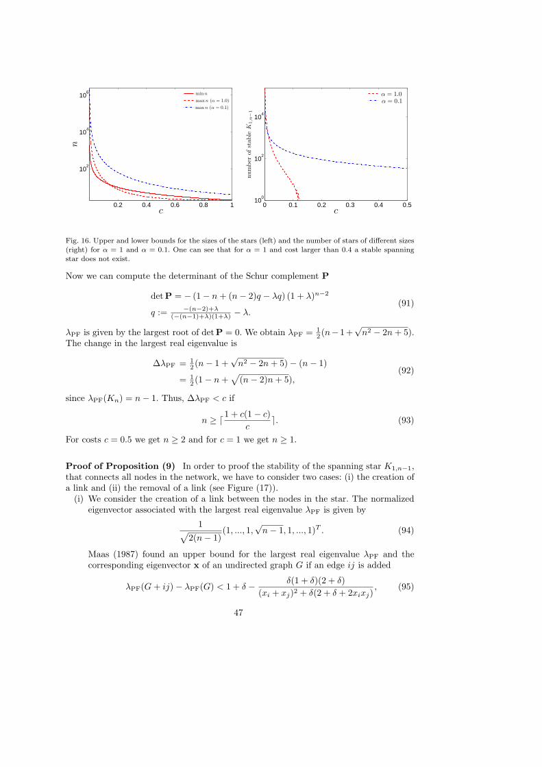
0.2 0.4 0.6 0.8 1

102

104

106

n

c

min n

max n (α = 1.0)

max n (α = 0.1)

0 0.1 0.2 0.3 0.4 0.510

0

102

104

num

ber

ofst

able

K1,n

−1

c

α = 1.0α = 0.1

Fig. 16. Upper and lower bounds for the sizes of the stars (left) and the number of stars of different sizes

(right) for α = 1 and α = 0.1. One can see that for α = 1 and cost larger than 0.4 a stable spanningstar does not exist.

Now we can compute the determinant of the Schur complement P

detP = − (1 − n + (n − 2)q − λq) (1 + λ)n−2

q := −(n−2)+λ

(−(n−1)+λ)(1+λ) − λ.(91)

λPF is given by the largest root of detP = 0. We obtain λPF = 12 (n− 1+

√n2 − 2n + 5).

The change in the largest real eigenvalue is

∆λPF = 12 (n − 1 +

√n2 − 2n + 5) − (n − 1)

= 12 (1 − n +

√

(n − 2)n + 5),(92)

since λPF(Kn) = n − 1. Thus, ∆λPF < c if

n ≥ ⌈1 + c(1 − c)

c⌉. (93)

For costs c = 0.5 we get n ≥ 2 and for c = 1 we get n ≥ 1.

Proof of Proposition (9) In order to proof the stability of the spanning star K1,n−1,that connects all nodes in the network, we have to consider two cases: (i) the creation ofa link and (ii) the removal of a link (see Figure (17)).

(i) We consider the creation of a link between the nodes in the star. The normalizedeigenvector associated with the largest real eigenvalue λPF is given by

1√

2(n − 1)(1, ..., 1,

√n − 1, 1, ..., 1)T . (94)

Maas (1987) found an upper bound for the largest real eigenvalue λPF and thecorresponding eigenvector x of an undirected graph G if an edge ij is added

λPF(G + ij) − λPF(G) < 1 + δ − δ(1 + δ)(2 + δ)

(xi + xj)2 + δ(2 + δ + 2xixj), (95)

47

(i)

(ii)

Fig. 17. A star K1,8 and (i) the creation of a link or (ii) the removal of a link.

where δ denotes the minimum degree in the graph G 29 . Applying Equation (95)to the star K1,n−1 gives ∆λPF = λPF(K1,n−1 + ij) − λPF(K1,n−1) < 2

n. The link

ij is not created if ∆λPF < c or equivalently

n >2

c. (96)

This is a decreasing function in c.(ii) The change in eigenvalue by removing a link from K1,n−1 is given by ∆λPF =

λPF(K1,n−1) − λPF(K1,n−2) =√

n − 1 −√

n − 2. A link is not removed from thestar if ∆λPF > c′ or equivalently

2 < n <1 + c′2(6 + c′2)

4c′2. (97)

Putting the bounds obtained in (i) and (ii) together we get the desired proposition. Thenumber of different sizes of stars that are stable are shown in Figure (5).

Proof of Proposition (11) A link between two disconnected firms is created if thelargest real eigenvalue of the connected component of the firms after the link is createdincreases more then the cost, i.e. ∆λPF > c. Similarly an existing link is removed if thelargest real eigenvalue of the connected component of the firms after the link is removeddoes not decrease more then the cost, i.e. |∆λPF| < c′ = αc, with c, c′, α ∈ [0, 1]. Wetherefore have to consider the change in eigenvalue by the creation or removal of a linkand compare it to the cost.

The proof of Proposition (11) is composed of two steps. (i) We show that in everyperiod t in the network formation process Γ(G) = G(0), G(1), ... the network G(t), t ≥ 1,consists only of graphs from the set S = {∅, P2, P3, P4}, where ∅ denotes the set of isolatednodes. (ii) We show that there exists a cycle, i.e. a sequence of repeatedly visited graphs,C = (P2, {P2, P2}, P4, P3), in which each graph is an improvement over the previousgraph in the sequence C (Jackson and Watts, 2002). Since all the graphs in the set Scan be found in the cycle C, starting from any of the graphs in S, the network formationprocess will proceed to the next graph in the cycle C. Therefore, for the given valuesof α and cost c, c′ respectively, we can infer that there does not exist a pairwise stableequilibrium network.

29Equation (95) is an upper bound and the number of stable stars derived from it may actually behigher.

48

(i) We give a proof by induction on the periods t ≥ 1 of the network formation processΓ(G). The induction basis is period t = 1. The network G(1) is obtained fromthe empty network G(0) = Kn (initial network) by the formation of a link andthus contains only a P2 and isolated nodes, both graphs are contained in the setS. Now we assume that the network at time t > 1 consist only of graphs in theset S (induction hypothesis). The induction step consists in showing from G(t) toG(t + 1), no other graphs than the ones in the set S will be created. This willconclude this part of the proof. In order to prove the induction step, we observethat in the network formation process Γ(G), at time t, a pair of nodes, say i andj, is selected at random. Either i and j are already connected in G(t) or they arenot. In any case, they both belong by assumption to one of the graphs in S. Allthe possible cases can be grouped as follows.(a) Both nodes are isolated. We show that the empty graph evolves into a P2. The

creation of a link between two isolated nodes results in ∆λPF = 1. Since byassumption c < 1, the link is indeed created.

(b) At least one of the nodes, say i, is part of a P2. In this case, we show that theonly possible evolution step is from two P2 to one P4.

(i) Link creation: Figure (18) shows all possible distinct graphs that can beobtained depending on which graph belongs the second node, j, and inwhich position. Each of these possible graphs is named with a numberin the following way. For instance, when j is in another P2, the possiblepositions in that P2 result both in one same graph labelled as 1. When jis in a P3, there are two possible distinct resulting graphs, labelled as 2.1and 2.2. Similarly, we label the graphs resulting in the remaining casethat j is in a P4. Table (2) report the increase of the largest eigenvalue ofthe graph when the link is created in all the possible cases. For instance,consider the graph 2.1 resulting from a P2 and a P3 with the creation of alink. Before the creation of the link, node i is in a P2 which has λPF = 1and node j is in a P3 graph which has λPF =

√2. Since the link formation

rule requires that both nodes will benefit after the creation of the link,we have to consider the worst case for the initial graph, which meansthe highest of the two values, i.e. λPF =

√2 = 1.414. For the resulting

graph 2.1 we have λ′PF =

√3 = 1.732, and therefore an increase of

eigenvalue ∆λPF = 0.318 which is smaller than the cost c = 0.586. Itfollows that this link will not be created. After analyzing all the othercases, we can see that only the case 1 results in an increase in the largestreal eigenvalue ∆λPF = 0.618 that is higher than the lower bound of thecost c > 2 −

√2 = 0.586. This implies that the only possible evolution

step at this point is the formation of one P4 starting from two P2. Noticethat P4 is in the set S.

(ii) Link deletion: A link is deleted if this beneficial to at least one of thetwo firms concurrent to the link, or, equivalently, if |∆λPF| < c′ = cα. Inthe case we are considering, by assumption at least one of the nodes isin a P2 and we examine the deletion of a link. This implies that the twonodes form a P2, which has λPF = 1. The deletion of the link impliesto evolve into an empty graph which has λPF = 0, yielding |∆λPF| = 1.Since, by assumption we have that c > 2−

√2, the case of cα > 1 implies

49

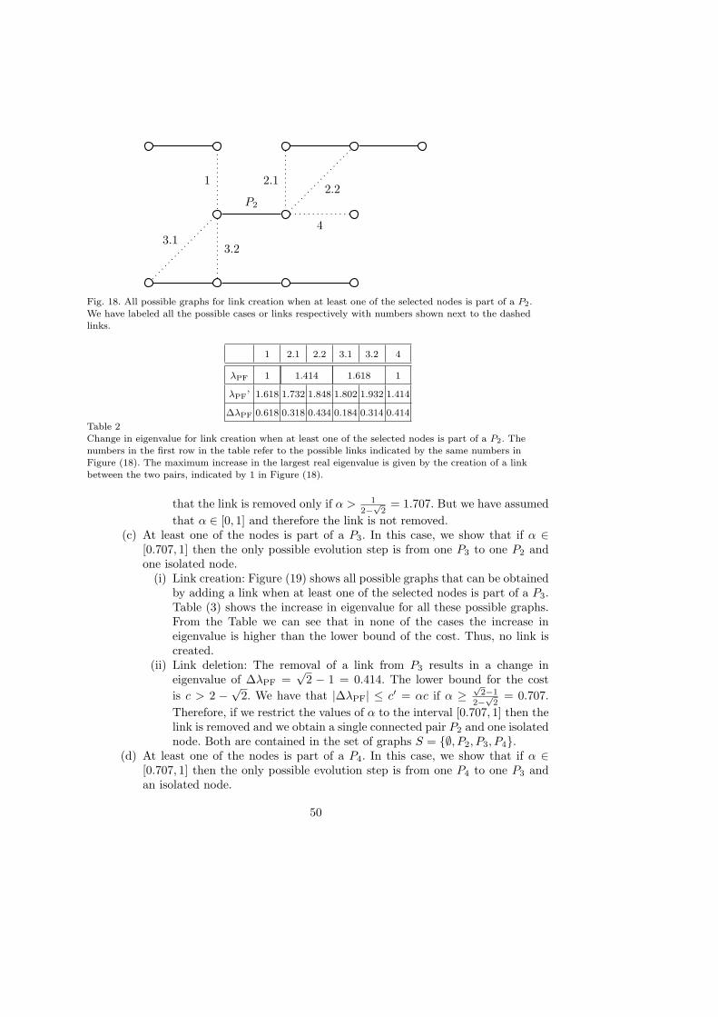
P2

3.13.2

4

1 2.12.2

Fig. 18. All possible graphs for link creation when at least one of the selected nodes is part of a P2.We have labeled all the possible cases or links respectively with numbers shown next to the dashedlinks.

1 2.1 2.2 3.1 3.2 4

λPF 1 1.414 1.618 1

λPF’ 1.618 1.732 1.848 1.802 1.932 1.414

∆λPF 0.618 0.318 0.434 0.184 0.314 0.414

Table 2Change in eigenvalue for link creation when at least one of the selected nodes is part of a P2. Thenumbers in the first row in the table refer to the possible links indicated by the same numbers in

Figure (18). The maximum increase in the largest real eigenvalue is given by the creation of a linkbetween the two pairs, indicated by 1 in Figure (18).

that the link is removed only if α > 12−

√2

= 1.707. But we have assumed

that α ∈ [0, 1] and therefore the link is not removed.(c) At least one of the nodes is part of a P3. In this case, we show that if α ∈

[0.707, 1] then the only possible evolution step is from one P3 to one P2 andone isolated node.

(i) Link creation: Figure (19) shows all possible graphs that can be obtainedby adding a link when at least one of the selected nodes is part of a P3.Table (3) shows the increase in eigenvalue for all these possible graphs.From the Table we can see that in none of the cases the increase ineigenvalue is higher than the lower bound of the cost. Thus, no link iscreated.

(ii) Link deletion: The removal of a link from P3 results in a change ineigenvalue of ∆λPF =

√2 − 1 = 0.414. The lower bound for the cost

is c > 2 −√

2. We have that |∆λPF| ≤ c′ = αc if α ≥√

2−12−

√2

= 0.707.

Therefore, if we restrict the values of α to the interval [0.707, 1] then thelink is removed and we obtain a single connected pair P2 and one isolatednode. Both are contained in the set of graphs S = {∅, P2, P3, P4}.

(d) At least one of the nodes is part of a P4. In this case, we show that if α ∈[0.707, 1] then the only possible evolution step is from one P4 to one P3 andan isolated node.

50

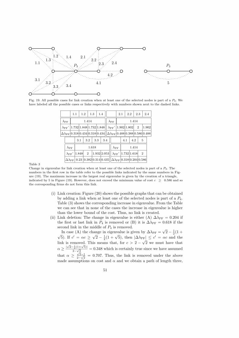
P3

3.13.2

3.3 3.4

1.11.3

1.2 1.4 2.1

2.32.2

2.4

4.2

4.1

P3

5

Fig. 19. All possible cases for link creation when at least one of the selected nodes is part of a P3. Wehave labeled all the possible cases or links respectively with numbers shown next to the dashed links.

1.1 1.2 1.3 1.4

λPF 1.414

λPF’ 1.732 1.848 1.732 1.848

∆λPF 0.318 0.434 0.318 0.434

2.1 2.2 2.3 2.4

λPF 1.414

λPF’ 1.902 1.802 2 1.902

∆λPF 0.488 0.388 0.586 0.488

3.1 3.2 3.3 3.4

λPF 1.618

λPF’ 1.848 2 1.932 2.053

∆λPF 0.23 0.382 0.314 0.435

4.1 4.2 5

λPF 1.414

λPF’ 1.732 1.618 2

∆λPF 0.318 0.204 0.586

Table 3Change in eigenvalue for link creation when at least one of the selected nodes is part of a P3. Thenumbers in the first row in the table refer to the possible links indicated by the same numbers in Fig-ure (19). The maximum increase in the largest real eigenvalue is given by the creation of a triangle,

indicated by 5 in Figure (19). However, does not exceed the minimum value of cost c ≥ 0.586 and sothe corresponding firms do not form this link.

(i) Link creation: Figure (20) shows the possible graphs that can be obtainedby adding a link when at least one of the selected nodes is part of a P4.Table (3) shows the corresponding increase in eigenvalue. From the Tablewe can see that in none of the cases the increase in eigenvalue is higherthan the lower bound of the cost. Thus, no link is created.

(ii) Link deletion: The change in eigenvalue is either (A) ∆λPF = 0.204 ifthe first or last link in P4 is removed or (B) it is ∆λPF = 0.618 if thesecond link in the middle of P4 is removed.

In case (A) the change in eigenvalue is given by ∆λPF =√

2 − 12 (1 +√

5). If c′ = αc ≥√

2 − 12 (1 +

√5), then |∆λPF| ≤ c′ = αc and the

link is removed. This means that, for c > 2 −√

2 we must have that

α ≥ |√

2− 12(1+

√5)|

2−√

2= 0.348 which is certainly true since we have assumed

that α ≥√

2−12−

√2

= 0.707. Thus, the link is removed under the above

made assumptions on cost and α and we obtain a path of length three,

51

P4

3.13.2 3.3

3.4

1.11.2

2.12.2 2.3

2.4

4.2

4.1

P4

5.1

5.2

Fig. 20. All possible cases for link creation when at least one of the selected nodes is part of a P4.

1.1 1.2

λPF 1.618

λPF’ 1.802 1.932

∆λPF 0.184 0.314

2.1 2.2 2.3 2.4

λPF 1.618

λPF’ 1.970 1.848 2.053 1.932

∆λPF 0.352 0.23 0.435 0.314

3.1 3.2 3.3 3.4

λPF 1.618

λPF’ 1.879 1.989 1.989 2.095

∆λPF 0.261 0.371 0.371 0.477

4.1 4.2

λPF 1.618

λPF’ 1.848 1.732

∆λPF

5.1 5.2

λPF 1.618

λPF’ 2.170 2

∆λPF 0.552 0.382

Table 4Change in eigenvalue for link creation when at least one of the selected nodes is part of a P4.

P3, which is in the set of graphs {∅, P2, P3, P4}.In case (B) we have that ∆λPF = 1− 1

2 (1 +√

5). This link is removed

for |∆λPF| ≤ c′ = cα implying that α ≥ |1− 12(1+

√5)|

2−√

2= 1.055. Since we

have assumed that α ∈ [0, 1] this cannot be true. Therefore, the link isnot removed.

Notice that in all the cases the graphs created belong to the set S, as wewanted to prove.

(ii) From the preceding analysis we can infer two facts: First, the individual profitsof the firms involved in the creation or removal of a link always increase alongthe closed sequence of graphs C = (P2, {P2, P2}, P4, P3.P2), as it is illustrated inFigure (8). Therefore, this is an improving path (Jackson and Watts, 2002) whichis cyclical and never reaches an equilibrium. Notice that, the firms responsible forthe creation or deletion of the links along the sequence are different and individualprofits of a given firm are not increasing at every step. Along the improving path,the individual profits of the firms involved in the link creation or removal increase,while the profits of the others may decrease. This highlights the effects of theexternalities inherent in our model on the individual profits of the firms.

Second, since at every step of the sequence there is only one possible networkevolution step and since all the non-empty graphs of the set S are also in the

52

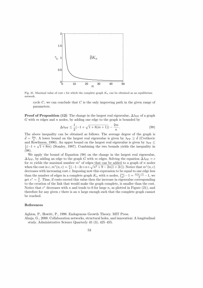
0 10 20 30 40 500

0.5

1

1.5

2

n

c∗ ∄Kn

Fig. 21. Maximal value of cost c for which the complete graph Kn can be obtained as an equilibriumnetwork.

cycle C, we can conclude that C is the only improving path in the given range ofparameters.

Proof of Proposition (12) The change in the largest real eigenvalue, ∆λPF of a graphG with m edges and n nodes, by adding one edge to the graph is bounded by

∆λPF ≤ 1

2(−1 +

√

1 + 8(m + 1)) − 2m

n. (98)

The above inequality can be obtained as follows. The average degree of the graph isd = 2m

n. A lower bound on the largest real eigenvalue is given by λPF ≥ d (Cvetkovic

and Rowlinson, 1990). An upper bound on the largest real eigenvalue is given by λPF ≤12 (−1 +

√1 + 8m) (Stanley, 1987). Combining the two bounds yields the inequality in

(98).We apply the bound of Equation (98) on the change in the largest real eigenvalue,

∆λPF, by adding an edge to the graph G with m edges. Solving the equation ∆λPF = cfor m yields the maximal number m∗ of edges that can be added to a graph of n nodeswhen the cost is c, m∗(n, c) = n

4 (−1−2c+n+√

n2 + 9 − 2n(1 + 2c)). Notice that m∗(n, c)decreases with increasing cost c. Imposing now this expression to be equal to one edge less

than the number of edges in a complete graph Kn with n nodes,(n2

)−1 = n(n−1)

2 −1, weget c∗ = 2

n. Thus, if costs exceed this value then the increase in eigenvalue corresponding

to the creation of the link that would make the graph complete, is smaller than the cost.Notice that c∗ decreases with n and tends to 0 for large n, as plotted in Figure (21), andtherefore for any given c there is an n large enough such that the complete graph cannotbe reached.

References

Aghion, P., Howitt, P., 1998. Endogenous Growth Theory. MIT Press.Ahuja, G., 2000. Collaboration networks, structural holes, and innovation: A longitudinal

study. Administrative Science Quarterly 45 (3), 425–455.

53

Aouchiche, M., Bell, F., Cvetkovic, D., Hansen, P., Rowlinson, P., Simic, S., Stevanovic,D., 2008. Variable neighborhood search for extremal graphs. 16. Some conjecturesrelated to the largest eigenvalue of a graph. European J. of Operational Research191 (3), 661–676.

Bala, V., Goyal, S., 2000. A noncooperative model of network formation. Econometrica68 (5), 1181–1230.

Ballester, C., Calvo-Armengol, A., Zenou, Y., 2006. Who’s who in networks. Wanted:The key player. Econometrica 74 (5), 1403–1417.

Bell, F., 1991. On the maximal index of connected graphs. Linear Algebra and its Ap-plications 144, 135–151.

Bollobas, B., 1998. Modern Graph Theory. Graduate Texts in Mathematics. Springer.Brualdi, R. A., Solheid, Ernie, S., 1986. On the spectral radius of connected graphs.

Publications de l’ Institute Mathmatique 53, 45–54.Burt, R., 1992. Structural Holes: The Social Structure of Competition. Harvard Univer-

sity Press, Cambridge, Massachussets.Carayol, N., Roux, P., YıldızoGlu, M., 2008. Inefficiencies in a model of spatial networks

formation with positive externalities. Journal of Economic Behavior and Organization67 (2), 495–511.

Coleman, J. S., 1988. Social capital in the creation of human capital. The AmericanJournal of Sociology 94, S95–S120.

Corbo, J., Calvo-Armengol, A., Parkes, D., 2006. A study of nash equilibrium in contri-bution games for peer-to-peer networks. SIGOPS Operation Systems Review 40 (3),61–66.

Cowan, R., Jonard, N., 2004. Network structure and the diffusion of knowledge. Journalof Economic Dynamics and Control 28 (8), 1557–1575.

Cowan, R., Jonard, N., 2007. Structural holes, innovation and the distribution of ideas.J. of Economic Interaction and Coordination 2, 93–110.

Cowan, R., Jonard, N., Zimmermann, J.-B., April 2006. Evolving networks of inventors.Journal of Evolutionary Economics 16 (1), 155–174.

Cvetkovic, D., Doob, M., Sachs, H., 1995. Spectra of Graphs: Theory and Applications.Johann Ambrosius Barth.

Cvetkovic, D., Rowlinson, P., 1990. The largest eigenvalue of a graph: A survey. Linearand Multilinear Algebra 28 (1), 3–33.

Cvetkovic, D., Rowlinson, P., Simic, S. K., 2007. Eigenvalue bound for the signless lapla-cian. Publications de l’institute mathematique, nouvelle serie 81 (95), 11–27.

Dosi, G., 1988. Sources, procedures and microeconomic effects of innovation. Journal ofEconomic Literature 26 (3), 1120–1171.

Fleming, L., King, C., Juda, Adam, I., 2007. Small worlds and regional innovation. Or-ganization Science 18 (6), 938–954.

Fruchterman, T., Reingold, E., 1991. Graph drawing by force-directed placement.Software- Practice and Experience 21 (11), 1129–1164.

Gargiulo, M., Benassi, M., 2000. Trapped in your own net? network cohesion, structuralholes, and the adaptation of social capital. Organization Science 11 (2), 183–196.

Goyal, S., Joshi, S., 2003. Networks of collaboration in oligopoly. Games and EconomicBehavior 43 (1), 57–85.

Goyal, S., Moraga-Gonzalez, J. L., 2001. R&D networks. RAND Journal of Economics32 (4), 686–707.

54

Gutman, I., Paule, P., 2002. The variance of the vertex degrees of randomly generatedgraphs. Univ. Beograd Publ. Elektrothen. Fak. 13, 30–35.

Haemers, W., 2006. Handbook of Linear Algebra. CRC Press, Ch. Matrices and Graphs.Hagedoorn, J., May 2002. Inter-firm R&D partnerships: an overview of major trends and

patterns since 1960. Research Policy 31 (4), 477–492.Haller, H., Kamphorst, J., Sarangi, S., 2007. (Non-)existence and scope of nash networks.

Economic Theory 31 (3), 597–604.Haller, H., Sarangi, S., 2005. Nash networks with heterogeneous links. Mathematical

Social Sciences 50 (2), 181–201.Hanaki, N., Nakajima, R., Ogura, Y., 2007. The dynamics of R&D collaboration in the

IT industry. Working paper.Hong, Y., 1993. Bounds of eigenvalues of graphs. Discrete Math. 123, 65–74.Horn, R. A., Johnson, C. R., 1990. Matrix Analysis. Cambridge University Press.Jackson, M. O., Golub, B., 2007. Naive learning in social networks: Convergence, influence

and wisdom of crowds. Working Papers 2007.64, Fondazione Eni Enrico Mattei.Jackson, M. O., Watts, A., 2002. The evolution of social and economic networks. Journal

of Economic Theory 106 (2), 265–295.Jackson, M. O., Wolinsky, A., 1996. A strategic model of social and economic networks.

Journal of Economic Theory 71 (1), 44–74.Kogut, B., Zander, U., August 1992. Knowledge of the firm, combinative capabilities,

and the replication of technology. Organization Science 3 (3), 383–397.Konig, M. D., Battiston, S., Napoletano, M., Schweitzer, F., 2008. On algebraic graph

theory and the dynamics of innovation networks. Networks and Heterogeneous Media3 (2), 201–219.

Letterie, W., Hagedoorn, J., van Kranenburg, H., Palm, F., May 2008. Information gath-ering through alliances. Journal of Economic Behavior & Organization 66 (2), 176–194.

Maas, C., 1987. Perturbation results for the adjacency spectrum of a graph. ZAMM67 (5), T428–T430.

Pammolli, F., Riccaboni, M., November 2002. Technological regimes and the growth ofnetworks: An empirical analysis. Small Business Economics 19 (3), 205–15.

Powell, W. W., Koput, K. W., Smith-Doerr, L., 1996. Interorganizational collaborationand the locus of innovation: Networks of learning in biotechnology. AdministrativeScience Quarterly 41 (1), 116–145.

Powell, W. W., White, D. R., Koput, K. W., Owen-Smith, J., 2005. Network dynamicsand field evolution: The growth of interorganizational collaboration in the life sciences.American Journal of Sociology 110 (4), 1132–1205.

Reinganum, J. F., 1983. Uncertain innovation and the persistence of monopoly. TheAmerican Economic Review 73 (4), 741–748.

Reinganum, J. F., 1985. Innovation and industry evolution. The Quarterly Journal ofEconomics 100 (1), 81–99.

Roijakkers, N., Hagedoorn, J., 2006. Inter-firm R&D partnering in pharmaceuticalbiotechnology since 1975: Trends, patterns, and networks. Research Policy 35 (3),431–446.

Rowley, T., Behrens, D., Krachhardt, D., 2000. Redundant governance structures: Ananalysis of structural and relational embeddness in the steel and semiconductor indus-tries. Strategic Management Journal 21 (3), 369–386.

Seneta, E., 2006. Non-negative Matrices And Markov Chains. Springer.

55

Stanley, R. P., 1987. A bound on the spectral radius of graphs with e edges. LinearAlgebra and its Applications 87, 267–269.

Stephenson, K., Zelen, M., 1989. Rethinking centrality: Methods and examples. SocialNetworks 11 (1), 1–37.

Vega-Redondo, F., 2007. Complex Social Networks. Series: Econometric Society Mono-graphs. Cambridge University Press.

Vega-Redondo, F., Goyal, S., 2007. Structural holes in social networks. Journal of Eco-nomic Theory 137 (1), 460–492.

Walker, G., Kogut, B., Shan, W., 1997. Social capital, structural holes and the formationof an industry network. Organization Science 8 (2), 109–125.

Wasserman, S., Faust, K., 1994. Social Network Analysis: Methods and Applications.Cambridge University Press.

Weitzman, M. L., 1998. Recombinant growth. The Quarterly Journal of Economics113 (2), 331–360.

West, Douglas, B., 2001. Introduction to Graph Theory, 2nd Edition. Prentice-Hall.Winter, S. G., 1984. Schumpeterian competition in alternative technological regimes.

Journal of Economic Behavior and Organization 5 (3), 287–320.Zwillinger, D., 1998. Handbook of Differential Equations. Academic Press.

56

Working Papers of the Center of Economic Research at ETH Zurich

(PDF-files of the Working Papers can be downloaded at www.cer.ethz.ch/research).

08/95 M. D. Konig, S. Battiston, M. Napoletano and F. SchweitzerThe Efficiency and Evolution of R&D Networks

08/94 H. Gersbach and F. MuheVote-Buying and Growth

08/93 H. GersbachBanking with Contingent Contracts, Macroeconomic Risks, and Banking Crises

08/92 J. DaubanesOptimal taxation of a monopolistic extractor: Are subsidies necessary?

08/91 R. WinklerOptimal control of pollutants with delayed stock accumulation

08/90 S. Rausch and T. F. RutherfordComputation of Equilibria in OLG Models with Many Heterogeneous Households

08/89 E. J. Balistreri, R. H. Hillberry and T. F. RutherfordStructural Estimation and Solution of International TradeModels with Heteroge-neous Firms

08/88 E. Mayer and O. GrimmCountercyclical Taxation and Price Dispersion

08/87 L. BretschgerPopulation growth and natural resource scarcity: long-run development under seem-ingly unfavourable conditions

08/86 M. J. Baker, C. N. Brunnschweiler, and E. H. BulteDid History Breed Inequality? Colonial Factor Endowments and Modern IncomeDistribution

08/85 U. von Arx and A. ZieglerThe Effect of CSR on Stock Performance: New Evidence for the USA and Europe

08/84 H. Gersbach and V. HahnForward Guidance for Monetary Policy: Is It Desirable?

08/83 I. A. MacKenzieOn the Sequential Choice of Tradable Permit Allocations

08/82 I. A. MacKenzie, N. Hanley and T. KornienkoA Permit Allocation Contest for a Tradable Pollution Permit Market

08/81 D. Schiess and R. WehrliThe Calm Before the Storm? - Anticipating the Arrival of General Purpose Tech-nologies

08/80 D. S. Damianov and J. G. BeckerAuctions with Variable Supply: Uniform Price versus Discriminatory

08/79 H. Gersbach, M. T. Schneider and O. SchnellerOn the Design of Basic-Research Policy

08/78 C. N. Brunnschweiler and E. H. BulteNatural Resources and Violent Conflict: Resource Abundance, Dependence and theOnset of Civil Wars

07/77 A. Schafer, S. ValenteHabit Formation, Dynastic Altruism, and Population Dynamics

07/76 R. WinklerWhy do ICDPs fail? The relationship between subsistence farming, poaching andecotourism in wildlife and habitat conservation

07/75 S. ValenteInternational Status Seeking, Trade, and Growth Leadership

07/74 J. Durieu, H. Haller, N. Querou and P. SolalOrdinal Games

07/73 V. HahnInformation Acquisition by Price-Setters and Monetary Policy

07/72 H. Gersbach and H. HallerHierarchical Trade and Endogenous Price Distortions

07/71 C. Heinzel and R. WinklerThe Role of Environmental and Technology Policies in the Transition to a Low-carbon Energy Industry

07/70 T. Fahrenberger and H. GersbachMinority Voting and Long-term Decisions

07/69 H. Gersbach and R. WinklerOn the Design of Global Refunding and Climate Change

07/68 S. ValenteHuman Capital, Resource Constraints and Intergenerational Fairness

07/67 O. Grimm and S. RiedMacroeconomic Policy in a Heterogeneous Monetary Union

07/66 O. GrimmFiscal Discipline and Stability under Currency Board Systems

07/65 M. T. SchneiderKnowledge Codification and Endogenous Growth

07/64 T. Fahrenberger and H. GersbachLegislative Process with Open Rules

07/63 U. von Arx and A. SchaferThe Influence of Pension Funds on Corporate Governance

07/62 H. GersbachThe Global Refunding System and Climate Change

06/61 C. N. Brunnschweiler and E. H. BulteThe Resource Curse Revisited and Revised: A Tale of Paradoxes and Red Herrings

06/60 R. WinklerNow or Never: Environmental Protection under Hyperbolic Discounting

06/59 U. Brandt-Pollmann, R. Winkler, S. Sager, U. Moslener and J.P. SchloderNumerical Solution of Optimal Control Problems with Constant Control Delays

06/58 F. MuheVote Buying and the Education of a Society

06/57 C. Bell and H. GersbachGrowth and Enduring Epidemic Diseases

06/56 H. Gersbach and M. MullerElections, Contracts and Markets

06/55 S. ValenteIntergenerational Transfers, Lifetime Welfare and Resource Preservation

06/54 H. Fehr-Duda, M. Schurer and R. SchubertWhat Determines the Shape of the Probability Weighting Function?

06/53 S. ValenteTrade, Envy and Growth: International Status Seeking in a Two-Country World

06/52 K. PittelA Kuznets Curve for Recycling

06/51 C. N. BrunnschweilerCursing the blessings? Natural resource abundance, institutions, and economicgrowth

06/50 C. Di Maria and S. ValenteThe Direction of Technical Change in Capital-Resource Economics

06/49 C. N. BrunnschweilerFinancing the alternative: renewable energy in developing and transition countries

06/48 S. ValenteNotes on Habit Formation and Socially Optimal Growth

06/47 L. BretschgerEnergy Prices, Growth, and the Channels in Between: Theory and Evidence

06/46 M. Schularick and T.M. StegerDoes Financial Integration Spur Economic Growth? New Evidence from the FirstEra of Financial Globalization