ISSN 2042-2695

CEP Discussion Paper No 1055

June 2011

Recursive Contracts

Albert Marcet and Ramon Marimon

Abstract We obtain a recursive formulation for a general class of contracting problems involving incentive constraints. These constraints make the corresponding maximization (sup) problems non recursive. Our approach consists of studying a recursive Lagrangian. Under standard general conditions, there is a recursive saddle-point (infsup) functional equation (analogous to a Bellman equation) that characterizes the recursive solution to the planner's problem and forward-looking constraints. Our approach has been applied to a large class of dynamic contractual problems, such as contracts with limited enforcement, optimal policy design with implementability constraints, and dynamic political economy models. Keywords: Transactional relationships, contracts and reputation, recursive formulation, participation constraint JEL Classifications: D80, L14 This paper was produced as part of the Centre’s Macro Programme. The Centre for Economic Performance is financed by the Economic and Social Research Council. Acknowledgements This is a substantially revised version of previously circulated papers with the same title (e.g. Marcet and Marimon 1998 and 1999). We would like to thank Fernando Alvarez, Truman Bewley, Edward Green, Robert Lucas, Andreu Mas-Colell, Fabrizio Perri, Edward Prescott, Victor Rios-Rull, Thomas Sargent, Robert Townsend and Jan Werner for comments on earlier developments of this work, all the graduate students who have struggled through a theory in progress and, in particular, Matthias Mesner and Nicola Pavoni for pointing out a problem overlooked in previous versions. Support from MCyT-MEyC of Spain, CIRIT, Generalitat de Catalunya and the hospitality of the Federal Reserve Bank of Minneapolis is acknowledged. Albert Marcet is an Associate of the Macro Programme at the Centre for Economic Performance and Lecturer in Economics, London School of Economics. Ramon Marimon is Director of the Max Weber Postdoctoral Programme and Professor of Economics at the European University Institute (EUI). He is also Chairman of the Barcelona Graduate School of Economics. Published by Centre for Economic Performance London School of Economics and Political Science Houghton Street London WC2A 2AE All rights reserved. No part of this publication may be reproduced, stored in a retrieval system or transmitted in any form or by any means without the prior permission in writing of the publisher nor be issued to the public or circulated in any form other than that in which it is published. Requests for permission to reproduce any article or part of the Working Paper should be sent to the editor at the above address. © A. Marcet and R. Marimon, submitted 2011

RECURSIVE CONTRACTS

Albert MarcetLondon School of Economics and CEP

Ramon MarimonEuropean University Institute and UPF - BarcelonaGSE

This version: March, 2011∗

Abstract

We obtain a recursive formulation for a general class of contractingproblems involving incentive constraints. These constraints make the cor-responding maximization (sup) problems non recursive. Our approachconsists of studying a recursive Lagrangian. Under standard generalconditions, there is a recursive saddle-point (infsup) functional equation(analogous to a Bellman equation) that characterizes the recursive solu-tion to the planner’s problem and forward-looking constraints. Our ap-proach has been applied to a large class of dynamic contractual problems,such as contracts with limited enforcement, optimal policy design withimplementability constraints, and dynamic political economy models.

1 Introduction

Recursive methods have become a basic tool for the study of dynamic economicmodels. For example, Stokey, et al. (1989) and Ljungqvist and Sargent (2004)describe a large number of macroeconomic models that can be analysed usingrecursive methods. A main advantage of this approach is that it characterizesoptimal decisions – at any time t – as time-invariant functions of a small set ofstate variables. In engineering systems, knowledge of the available technologyand of the current state is enough to decide the optimal control, since currentreturns and the feasible set depend only on past and current predeterminedvariables. In this case the value of future states is assessed by the value function∗This is a substantially revised version of previously circulated papers with the same title

(e.g. Marcet and Marimon 1998 & 1999). We would like to thank Fernando Alvarez, TrumanBewley, Edward Green, Robert Lucas, Andreu Mas-Colell, Fabrizio Perri, Edward Prescott,Victor Rios-Rull, Thomas Sargent, Robert Townsend and Jan Werner for comments on earlierdevelopments of this work, all the graduate students who have struggled through a theory inprogress and, in particular, Matthias Mesner and Nicola Pavoni for pointing out a problemoverlooked in previous versions. Support from MCyT-MEyC of Spain, CIRIT, Generalitat deCatalunya and the hospitality of the Federal Reserve Bank of Minneapolis is acknowledged.

1

and, under standard dynamic programming assumptions, the Bellman equationis satisfied and a standard recursive formulation is obtained.

However, one key assumption to obtain the Bellman equation is that futurechoices do not constrain the set of today’s feasible choices. Unfortunately, thisassumption does not hold in many interesting economic problems. For example,in contracting problems where agents are subject to intertemporal participation,or other intertemporal incentive constraints, the future development of the con-tract determines the feasible action today. Similarly, in models of optimal pol-icy design agents’ reactions to government policies are taken as constraints and,therefore, future actions limit the set of current feasible actions available to thegovernment. Many dynamic games – for example, dynamic political-economymodels – share the same feature that an agent’s current feasible actions dependon functions of future actions.

In general, in the presence of forward-looking constraints – as in rationalexpectations models where agents commit to contracts subject to incentive con-straints (e.g. commitment may be limited) – optimal plans, or contracts, do notsatisfy the Bellman equation and the solution is not recursive in the standardsense. In this paper we provide an integrated approach for a recursive formu-lation of a large class of dynamic models with forward-looking constraints byreformulating them as equivalent recursive saddle-point problems.

Our approach has a wide range of applications. In fact, it has already provedto be useful in the study of very many models1. Just to mention a few exam-ples: growth and business cycles with possible default (Marcet and Marimon(1992), Kehoe and Perri (2002), Cooley, et al. (2004)); social insurance (At-tanasio and Rios-Rull (2000)); optimal fiscal and monetary policy design withincomplete markets (Aiyagari, Marcet, Sargent and Seppala (2002), Svenssonand Williams (2008)), and political-economy models (Acemoglu, Golosov andTsyvinskii (2011)). For brevity, however, we do not present further applicationshere and limit the presentation of the theory to the case of full information.

We build on traditional tools of economic analysis such as duality theoryof optimization, fixed point theory, and dynamic programming. We proceed inthree steps. We first study the planner’s problem with incentive constraints(PP) as an infinite-dimensional maximization problem, and we embed thisproblem in a more general class of planner’s problems (PPµ); these problemsare parameterized by the weight (µ) of a (Benthamite) social welfare function,which accounts for the functions appearing in the constraints with future con-trols (forward-looking constraints). The objective function of PPµ is similar toPareto-optimal problems where µ is the vector of weights given to the differentinfinitely-lived agents in the economy.

Second, we consider the Lagrangean which incorporates the forward-lookingconstraints of the first period, which defines our starting saddle-point planner’sproblem (SPPµ) and we prove a duality result between this saddle-point prob-lem and the planner’s problem (PPµ). This construction helps to characterize

1As we write this version google scholar reports that the working paper has been cited 290times, many of these citations are applications of the method.

2

the ‘non-recursivity problem’and provides a key step towards its resolution.As it is well known, the solution of dynamic models with forward-looking

constraints is, in general, time-inconsistent, in the following sense: if at someperiod t > 0 the agent solves PPµ for the whole future path given the state vari-ables found at t, the agent will not choose the path that he had chosen in periodzero (unless, of course, the forward-looking constraints are not binding, up toperiod t). This ‘non-recursivity problem’problem is at the root of the difficultiesin expressing the optimal solution with a time-invariant policy function.

A key insight of our approach is to show that there is a modified problemPPµ′ such that if the agent reoptimizes this problem at t = 1 for a certain µ′,the solution from period t = 1 onwards is the same that had been prescribedby PPµ from the standpoint of period zero. The key is to choose the weightsµ′ appropriately. We show that the appropriate µ′ is given by the lagrangemultipliers of SPPµ in period zero. This procedure of sequentially connect-ing saddle-point problems is well defined and it is recursive when solutions areunique. The problem PPµ′ can be thought of as the‘continuation problem’thatneeds to be solved each period in order to implement the constrained-efficientsolution. It supports our claim that the recursive formulation is obtained by in-troducing the vector µ, summarizing the evolution of the Lagrange multipliers,as co-state variable in a time-invariant policy function. As a result, with ourmethod it is easy to guarantee existence of the solution to PPµ′ for any µ′ ≥ 0,making the practical implementation of this method not more complicated thanstandard dynamic programming problems.

Third, we extend dynamic programming theory to show that the sequenceof modified saddle-point problems (SPPµt

) satisfies a saddle-point functionalequation (SPFE; a saddle-point Bellman equation) and, conversely, that policiesobtained from solving the saddle-point functional equation (SPFE) provide asolution to the original SPPµ and, therefore, to the PPµ problem. This lattersufficiency result is very general; in particular, it does not rely on convexityassumptions. This is important because incentive constraints do not have aconvex structure in many applications. However, this result is limited in thatwe assume (local) uniqueness of solutions. We discuss the role this assumptionplays and, in particular, we show how our approach, and results, do not dependon this assumption.

In addition, we also show how standard dynamic programming results, basedon a contraction mapping theorem, generalize to our saddle-point functionalequation (SPFE). An immediate consequence of these results is that one canuse standard computational techniques that have been used to solve dynamicprogramming problems – such as solution of first-order-conditions for a givenrecursive structure of the policy function, or value function iteration – to solvedynamic saddle-point problems. Not only the computational techniques neededbut also our assumptions are standard in dynamic economic models.

Our approach is related to other existing approaches that study dynamicmodels with expectations constraints, in particular to the pioneering works ofAbreu, Pearce and Stacchetti (1990), Green (1987) and Thomas and Worrall(1988), and the applications that have followed. We briefly discuss how these,

3

and other, works relate to ours in Section 6, after presenting the main bodyof the theory in Sections 4 and 5. Section 2 provides a basic introduction toour approach and Section 3 a couple of canonical examples (most proofs arecontained in the Appendix).

2 Formulating contracts as recursive saddle-pointproblems

In this section we give an outline of our approach, leaving the technical detailsand proofs for sections 4 and 5. Our interest is to solve problems that have thefollowing representation:

PP sup{at,xt}

E0

∞∑t=0

βtr(xt, at, st) (1)

s.t. xt+1 = `(xt, at, st+1), p(xt, at, st) ≥ 0, t ≥ 0 (2)

EtNj+1∑n=1

βnhj0(xt+n, at+n, st+n) + hj1(xt, at, st) ≥ 0, j = 1, ...l, t ≥ 0

(3)

x0 = x, s0 = s,

at is measurable with respect to (. . . , st−1, st).

where r, `, p, h0, h1 are known functions, β, x, s known constants, {st}∞t=0 anexogenous stochastic Markov process, Nj = ∞ for j = 0, ..., k, and Nj = 0 forj = k + 1, ..., l.

Standard dynamic programming methods only consider constraints of form(2) (see, for example, Stokey, et al. (1989) and Cooley, (1995)). Constraintsof form (3) are not a special case of (2), since they involve expected valuesof future variables2. We know from Kydland and Prescott (1977) that, underthese constraints, the usual Bellman equation is not satisfied, the solution isnot, in general, of the form at = f(xt, st) for all t, and the whole history ofpast shocks st can matter for today’s optimal decision. By letting Nj = ∞PP covers a large class of problems where discounted present values enter theimplementability constraint. For example, long term contracts with intertem-poral participation constraints take this form.3 Alternatively, by letting Nj = 0PP covers problems where intertemporal reactions of agents must be takeninto account. For example, dynamic Ramsey problems, where the government

2One might think that expressing (3) in the form v(xt, st)− ψ(xt, st) ≥ 0, where v is thediscounted sum Et

P∞n=0 β

nh0(xt+n, at+n, st+n), xt, at, st) and ψ = h1 − h0 converts (3)into (2). But this does not solve the problem since v is not known a priori.

3Combining (2) and (3) accounts for a broad class of constraints. For example, a nonlinearparticipation constraint of the form g(Et

P∞n=0 β

nh(xt+n, at+n, st+n), xt, at, st) ≥ 0 caneasily be incorporated in our framework with one constraint of the form (2), g(wt, xt, at, st) ≥0 (with control variables (wt, at)), and one of the form (3), Et

P∞n=0 β

nh(xt+n, at+n, st+n)= wt.

4

chooses policy variables subject to optimal dynamic behavior by the agents inthe economy, have this form4. Even though we focus on the two canonical casesNj = ∞ and Nj = 0, intermediate cases can be easily incorporated. It is thenwithout loss of generality that we let Nj = ∞, for j = 0, ..., k, and Nj = 0 forj = k + 1, ..., l.

A first step of our approach is to consider a more general class of problems,parameterized by µ:

PPµ sup{at,xt}

E0

l∑j=0

Nj∑t=0

βtµjhj0(xt, at, st)

s.t. xt+1 = `(xt, at, st+1), p(xt, at, st) ≥ 0, (4)

EtNj+1∑n=1

βnhj0(xt+n, at+n, st+n) + hj1(xt, at, st) ≥ 0, t ≥ 0, (5)

x0 = x, s0 = s (6)and at is measurable with respect to (. . . , st−1, st).

The main difference with PP is that in PPµ we have incorporated the hj0functions of the forward-looking constraints (3) into the objective function. Also,the superindex j now starts from j = 0, with h0

0,, to account for the rewardfunction of the original problem. More precisely, if we let h0

0 = r, we setµ = (1, 0, ..., 0) and we choose a very large h0

1 to guarantee that (5) is neverbinding for j = 0, PPµ is the original PP. Furthermore, it should also benoticed that the value function of this problem, when well defined – say, Vµ(x, s)– is homogeneous of degree one in µ; a property that our approach exploits (andthe reason for collecting in the objective function the original return function rof PP, together with the forward-looking elements of the constraints).

Notice that PPµ is an infinite-dimensional maximization problem which,under relatively standard assumptions, is guaranteed to have a solution forarbitrary µ ≥ 0. The solution is a plan5 a ≡ {at}t=0, where at(. . . , st−1, st) is astate-contingent action (Proposition 1).

An intermediate step in our approach is to transform program PPµ into asaddle-point problem in the following way. Consider writing the Lagrangean forPPµ when a lagrange multiplier γ ∈ Rl+1 is attached to the forward-lookingconstraints only in period t = 0 and the remaining constraints for t > 0 are left

4See Section 6 for references to related work using constraints of the form Nj = ∞ andNj = 0.

5We use the bold notation to denote sequences of measurable functions.

5

as constraints. The Lagrangean then is

L(a,γ;µ) = E0

l∑j=0

Nj∑t=0

βtµjhj0(xt, at, st) + (7)

l∑j=0

γj

E0

Nj+1∑t=1

βthj0(xt, at, st) + hj1(x0, a0, s0)

. (8)

If we find a saddle-point of L subject to (4) for all t ≥ 0 and (5) for all t ≥ 1,the usual equivalences between this saddle-point and the optimal allocation ofPPµ can be exploited. Using simple algebra it is easy to show that L can berewritten as the objective function in the following saddle point problem6:

SPPµ infγ∈Rl+1

+

sup{at,xt}

µh0(x0, a0, s0) + γh1(x0, a0, s0)

+ β E0

l∑j=0

ϕj(µ, γ)Nj∑t=0

βt hj0(xt+1, at+1, st+1) (9)

s.t. xt+1 = `(xt, at, st+1), p(xt, at, st) ≥ 0, t ≥ 0

EtNj+1∑n=1

βnhj0(xt+n, at+n, st+n) + hj1(xt, at, st) ≥ 0, j = 0, ..., l, t ≥ 1

for initial conditions x0 = 0 and s0 = s, where ϕ is defined as

ϕj(µ, γ) ≡ µj + γj if Nj =∞, i.e. j = 0, ..., k≡ γj if Nj = 0, i.e. j = k + 1, ..., l.

The usefulness of SPPµ comes from the fact that its objective function has avery special form: the term inside the expectation in (9) is precisely the objectivefunction of PPϕ(µ, γ∗) given the states (x∗1, s1). This will allow us to show thatif ({a∗t }∞t=0, γ

∗) solves SPPµ for initial conditions (x, s) then {a∗t+1}∞t=0 solvesPPϕ(µ, γ∗) given initial conditions (x∗1, s1), where x∗1 = `(x0, a

∗0, s1). That is,

the continuation problem that needs to be solved in the next period is preciselya planner problem where the weights have been shifted according to ϕ.

We then show that, under fairly general conditions, solutions to PPµ aresolutions to SPPµ (Theorem 1), and viceversa (Theorem 2). Also, the usualslackness conditions will guarantee that if ({a∗t }, γ∗) solves SPPµ

E0

l∑j=0

γj∗

Nj+1∑t=1

βthj0(x∗t , a∗t , st) + hj1(x, a∗0, s)

= 0, (10)

so that the values achieved by the objective functions of SPPµ and PPµ coin-cide.

6We use the notation µh0(x, a, s) ≡Plj=0 µ

jhj0(x, a, s).

6

If PPµ were a standard dynamic programming problem (i.e. without (5)),then the following Bellman equation would be satisfied:

Vµ(x, s) = supa{µh0(x, a, s) + β E [Vµ(`(x, a, s′), s′) | s]} (11)

s.t. p(x, a, s) ≥ 0.

The reason that the Bellman equation holds is that in standard dynamicprogramming if PPµ is reoptimized at period t = 1 given initial conditions(x∗1, s1), the reoptimization simply confirms the choice that had been previouslymade for t ≥ 1. However, with forward-looking constraints (5) this Bellmanequation is not satisfied, the reason being that if the problem is reoptimized att = 1 the choice will violate the forward looking constraint of period t = 0, if (5)is binding at t = 0. A central element of our approach is that, as suggested by theobjective function of SPPµ, if the solution is reoptimized in period t = 1 withthe new weights µ′ = ϕ(µ, γ∗) – that is, if in period one the reoptimization isfor the problem PPµ′ , – the result confirms the solution of the original problemPPµ. This allows the construction of a recursive formulation of our originalPPµ problem where the value function with modified weights is included in theright-hand side of a functional ‘Bellman-like’equation to capture the terms in(9). More specifically, we show that under fairly general assumptions solutionsto SPPµ obey a saddle-point functional equation (SPFE). More specifically,we look for functions W that satisfy the following

SPFE W (x, µ, s) = infγ≥0

supa{µh0(x, a, s) + γh1(x, a, s) + β E [W (x′, µ′, s′)| s]}

s.t. x′ = `(x, a, s′), p(x, a, s) ≥ 0and µ′ = ϕ(µ, γ),

and we show that this holds for W (x, µ, s) = Vµ(x, s) (Theorem 3).We only consider problems where the infsup problem has unique optimal

choices.7 In this case optimal allocations and multipliers are uniquely deter-mined and there is a policy function ψ; i.e. ( a∗, γ∗) = ψ(x, µ, s) associatedwith a value function W satisfying SPFE. Finally we show that the followingrecursive formulation

( a∗t , γ∗t ) = ψ(x∗t , µ

∗t , st)

µ∗t+1 = ϕ(µ∗t , γ∗t )

gives the optimal policy we are seeking. More precisely, we first show that, given{a∗t , γ∗t } generated by ψ for initial conditions (x, µ, s), ({a∗t }∞t=0, γ

∗0)solves SPPµ

in state (x, s), that ({a∗t }∞t=1, γ∗1) solves SPPµ∗1

in state (x∗1, s1), etc. (Theorem4). As a result, the path {a∗t } for µ0 = (1, 0, ...0) is a solution to PP.

In this sense, the modified problem PPµ is the ‘correct continuation problem’to the planners’ problem: if µ is properly updated, the solution can be foundeach period by re-optimizing PPµ∗t

.7We discuss this issue in more detail in Sections 4 and 5.

7

2.1 The Principle of Optimality with forward-looking con-straints

Our central result is not a simple restatement of the standard dynamic program-ming principle of optimality to our saddle-point formulation8. This principlesays (when there are no forward-looking constraints)9: if Vµ satisfies the Bell-man equation (11), evaluated at (x, s)), it is the (sup) value of PPµ, whenthe initial state is (x, s), and a sequence {a∗t }∞t=1 solves PPµ if and only if itsatisfies:

Vµ(x∗t , st) = µh0(x∗t , a∗t , s) + βE

[Vµ(x∗t+1, st+1)| st

]x∗t+1 = `(x∗t , a

∗t , st+1), x∗t = x.

In our context, under standard assumptions it is true that if {a∗t }∞t=1 solves PPµ

when the initial state is (x, s) and attains the value Vµ(x, s), then W (x, µ, s) ≡Vµ(x, s) and

W (x∗t , µ∗t , st) = µ∗th0(x∗t , a

∗t , st) + γ∗th1(x∗t , a

∗t , st) + β E

[W (x∗t+1, µ

∗t+1, st+1)| st

](12)

x∗t+1 = `(x∗t , a∗t , st+1), x∗t = x

µ∗t+1 = ϕ(µ∗t , γ∗t ), µ

∗0 = (1, 0, ..., 0),

where {γ∗t }∞t=1 is the sequence of Lagrange multipliers associated with the se-quence of SPPµ (Theorems 1 and 3).

However, the converse, sufficiency, theorem that ifW (x, µ, s) satisfies SPFEand ({a∗t }∞t=1, {γ∗t }∞t=1) satisfies (12) then Vµ(x, s) ≡ W (x, µ, s) is the value ofPPµ and {a∗t }∞t=1 solves PPµ is true if, in addition, W (x, µ, s) = µω(x, µ, s)and

ωj(x∗t , µ∗t , st) = hj0(x∗t , a

∗t , st) + β E

[ωj(x∗t+1, µ

∗t+1, st+1)| st

], (13)

if j = 0, ..., k, andωj(x∗t , µ

∗t , st) = hj0(x∗t , µ

∗t , st) if j = k + 1, ..., l. (14)

These recursive equations for the forward-looking constraints are needed toguarantee that these constraints are also satisfied in the original PPµ. Noticethat if W (x, µ, s) is differentiable in µ then, by Euler’s Theorem, W (x, µ, s) =µω(x, µ, s) (where ωj ≡ ∂µjW ) and equations (13) and (14) follow from theEnvelope Theorem. We show, and use, the fact that if {a∗t }∞t=1 is unique (atleast locally unique) then W (x, µ, s) is differentiable in µ and, therefore, werecover the Principle of Optimality for our saddle-point formulation (Theo-

8This subsection clarifies our approach and what is new with respect of our previous work;it can be skipped by the reader only interested in how our approach works and on our mainresults.

9See, for example, Stokey et al (1989).

8

rems 4 and 5), without having to impose equations (13) and (14) as ‘promise-keeping’constraints10.

Before we turn to these results in Sections 4 and 5, in the next Section weshow how our approach is implemented in a couple of canonical examples.

3 Two Examples

In this Section we illustrate our approach with two examples. In the first, thereare only intertemporal participation constraints so it is a case when Nj =∞ (i.e.k = l); in the second, there are only intertemporal one-period (Euler) constraintshence it is a case with Nj = 0 (i.e. k = 0). The first is similar to the modelstudied in Marcet and Marimon (1992), Kocherlakota (1996), Kehoe and Perri(2002), among others, and it is canonical of models with intertemporal defaultconstraints; the second is based on the model studied by Aiyagari et al. (2002)and it is a canonical model with Euler constraints, as in Ramsey equilibria ofoptimal fiscal and monetary policy.

3.1 Intertemporal participation constraints.

We consider, as an example, a model of a partnership, where several agentscan share their individual risks and jointly invest in a project which can notbe undertaken by single (or subgroups of) agents. Formally, there is a singlegood and J infinitely-lived consumers. Preferences of agent j are represented byE0

∑∞t=0 β

t u(cjt ); u is assumed to be bounded, strictly concave and monotone,with u(0) = 0; c represents individual consumption. Agent j receives an endow-ment of consumption good yjt at time t and, given a realization of the vector ytagent j has an outside option that delivers total utility vaj (yt) if he leaves thecontract in period t, where vaj is some known function. It is often assumed that

the outside option is the autarkic solution: vaj (yt) = E[∑∞

n=0 βn u(yjt+n) | yjt

],

which implicitly assumes that if agent j defaults in period t he is permanentlyexcluded from the partnership and he does not have any claims on the produc-tion and the capital of the partnership in, and after, period t.

Total production is given by F (k, θ), and it can be split into consumption cand investment i. The stock of capital k depreciates at the rate δ. The joint pro-cess {θt, yt}∞t=0 is assumed to be Markovian and the initial conditions (k0, θ0, y0)are given. The planner looks for pareto optimal allocations that ensure that noagent ever leaves the contract. Letting Yt =

∑Jj=1 y

jt > 0 the planner’s problem

10In our previous work (Marcet and Marimon (1998, 1999)) we assumed uniqueness ofsolutions and used the fact that the contraction mapping guarantees the uniqueness of thevalue function. Messner and Pavoni (2004) showed how the principle of optimality could failin our context when solutions are not unique. The missing element being the recursivity of theforward-looking constraints. The above statement of the principle of optimality for problemswith forward-llooking constraints and, correspondingly, our sufficiency theorems address thisissue, which we further discuss in Section 6.

9

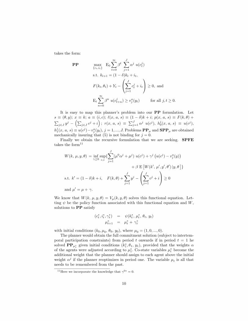
takes the form:

PP max{ct,it}

E0

∞∑t=0

βtJ∑j=1

αj u(cjt )

s.t. kt+1 = (1− δ)kt + it,

F (kt, θt) + Yt −

J∑j=1

cjt + it

≥ 0, and

Et∞∑n=0

βn u(cjt+n) ≥ vaj (yt) for all j, t ≥ 0.

It is easy to map this planner’s problem into our PP formulation. Lets ≡ (θ, y); x ≡ k; a ≡ (i, c); `(x, a, s) ≡ (1 − δ)k + i; p(x, a, s) ≡ F (k, θ) +∑j∈J y

j −(∑

j∈J cj + i

); r(x, a, s) ≡

∑Jj=1 α

j u(cj), hj0(x, a, s) ≡ u(cj),

hj1(x, a, s) ≡ u(cj)−vaj (yt), j = 1, ..., J. Problems PPµ and SPPµ are obtainedmechanically insuring that (5) is not binding for j = 0.

Finally we obtain the recursive formulation that we are seeking. SPFEtakes the form11

W (k, µ, y, θ) = infγ≥0

supc,i{J∑j=1

(µ0αj + µj) u(cj) + γj(u(cj)− vaj (y)

)+ β E

[W (k′, µ′, y′, θ′) |y, θ

]}

s.t. k′ = (1− δ)k + i, F (k, θ) +J∑j=1

yj −

J∑j=1

cj + i

≥ 0

and µ′ = µ+ γ.

We know that W (k, µ, y, θ) = Vµ(k, y, θ) solves this functional equation. Let-ting ψ be the policy function associated with this functional equation and W ,solutions to PP satisfy

(c∗t , i∗t , γ∗t ) = ψ(k∗t , µ

∗t , θt, yt)

µ∗t+1 = µ∗t + γ∗t

with initial conditions (k0, µ0, θ0, y0), where µ0 = (1, 0, ..., 0).The planner would obtain the full commitment solution (subject to intertem-

poral participation constraints) from period t onwards if in period t = 1 hesolved PPµ∗1

given initial conditions (k∗1 , θ1, y1), provided that the weights αof the agents were adjusted according to µ∗1. Co-state variables µ∗t become theadditional weight that the planner should assign to each agent above the initialweight αj if the planner reoptimizes in period one. The variable µt is all thatneeds to be remembered from the past.

11Here we incorporate the knowledge that γ0∗ = 0.

10

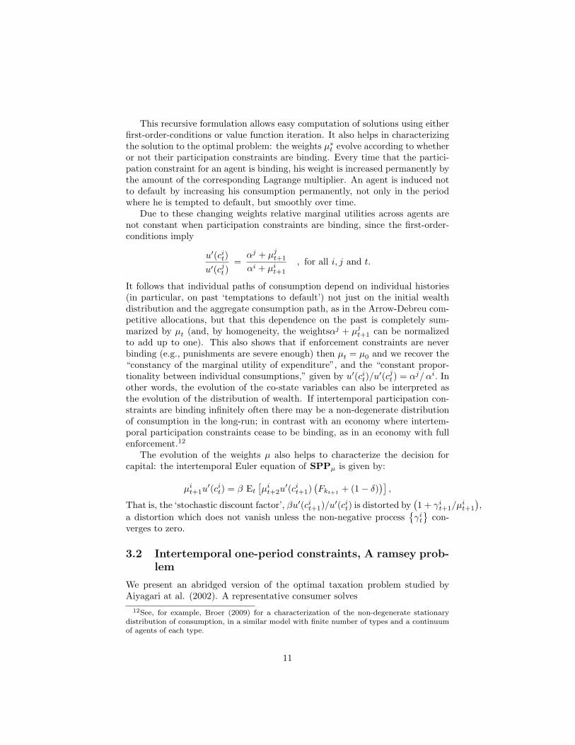
This recursive formulation allows easy computation of solutions using eitherfirst-order-conditions or value function iteration. It also helps in characterizingthe solution to the optimal problem: the weights µ∗t evolve according to whetheror not their participation constraints are binding. Every time that the partici-pation constraint for an agent is binding, his weight is increased permanently bythe amount of the corresponding Lagrange multiplier. An agent is induced notto default by increasing his consumption permanently, not only in the periodwhere he is tempted to default, but smoothly over time.

Due to these changing weights relative marginal utilities across agents arenot constant when participation constraints are binding, since the first-order-conditions imply

u′(cit)u′(cjt )

=αj + µjt+1

αi + µit+1

, for all i, j and t.

It follows that individual paths of consumption depend on individual histories(in particular, on past ‘temptations to default’) not just on the initial wealthdistribution and the aggregate consumption path, as in the Arrow-Debreu com-petitive allocations, but that this dependence on the past is completely sum-marized by µt (and, by homogeneity, the weightsαj + µjt+1 can be normalizedto add up to one). This also shows that if enforcement constraints are neverbinding (e.g., punishments are severe enough) then µt = µ0 and we recover the“constancy of the marginal utility of expenditure”, and the “constant propor-tionality between individual consumptions,” given by u′(cit)/u

′(cjt ) = αj/αi. Inother words, the evolution of the co-state variables can also be interpreted asthe evolution of the distribution of wealth. If intertemporal participation con-straints are binding infinitely often there may be a non-degenerate distributionof consumption in the long-run; in contrast with an economy where intertem-poral participation constraints cease to be binding, as in an economy with fullenforcement.12

The evolution of the weights µ also helps to characterize the decision forcapital: the intertemporal Euler equation of SPPµ is given by:

µit+1u′(cit) = β Et

[µit+2u

′(cit+1)(Fkt+1 + (1− δ)

)],

That is, the ‘stochastic discount factor’, βu′(cit+1)/u′(cit) is distorted by(1 + γit+1/µ

it+1

),

a distortion which does not vanish unless the non-negative process{γit}

con-verges to zero.

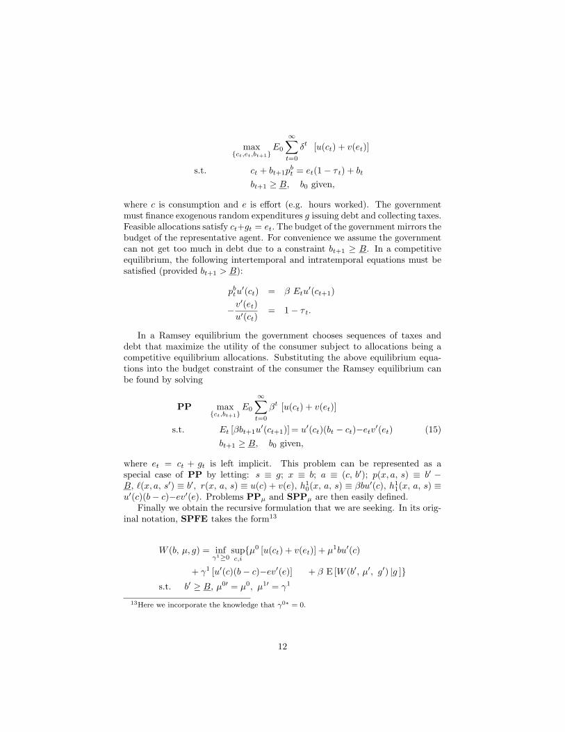
3.2 Intertemporal one-period constraints, A ramsey prob-lem

We present an abridged version of the optimal taxation problem studied byAiyagari at al. (2002). A representative consumer solves

12See, for example, Broer (2009) for a characterization of the non-degenerate stationarydistribution of consumption, in a similar model with finite number of types and a continuumof agents of each type.

11

max{ct,et,bt+1}

E0

∞∑t=0

δt [u(ct) + v(et)]

s.t. ct + bt+1pbt = et(1− τ t) + bt

bt+1 ≥ B, b0 given,

where c is consumption and e is effort (e.g. hours worked). The governmentmust finance exogenous random expenditures g issuing debt and collecting taxes.Feasible allocations satisfy ct+gt = et. The budget of the government mirrors thebudget of the representative agent. For convenience we assume the governmentcan not get too much in debt due to a constraint bt+1 ≥ B. In a competitiveequilibrium, the following intertemporal and intratemporal equations must besatisfied (provided bt+1 > B):

pbtu′(ct) = β Etu

′(ct+1)

−v′(et)u′(ct)

= 1− τ t.

In a Ramsey equilibrium the government chooses sequences of taxes anddebt that maximize the utility of the consumer subject to allocations being acompetitive equilibrium allocations. Substituting the above equilibrium equa-tions into the budget constraint of the consumer the Ramsey equilibrium canbe found by solving

PP max{ct,bt+1}

E0

∞∑t=0

βt [u(ct) + v(et)]

s.t. Et [βbt+1u′(ct+1)] = u′(ct)(bt − ct)−etv′(et) (15)

bt+1 ≥ B, b0 given,

where et = ct + gt is left implicit. This problem can be represented as aspecial case of PP by letting: s ≡ g; x ≡ b; a ≡ (c, b′); p(x, a, s) ≡ b′ −B, `(x, a, s′) ≡ b′, r(x, a, s) ≡ u(c) + v(e), h1

0(x, a, s) ≡ βbu′(c), h11(x, a, s) ≡

u′(c)(b− c)−ev′(e). Problems PPµ and SPPµ are then easily defined.Finally we obtain the recursive formulation that we are seeking. In its orig-

inal notation, SPFE takes the form13

W (b, µ, g) = infγ1≥0

supc,i{µ0 [u(ct) + v(et)] + µ1bu′(c)

+ γ1 [u′(c)(b− c)−ev′(e)] + β E [W (b′, µ′, g′) |g ]}s.t. b′ ≥ B, µ0′ = µ0, µ1′ = γ1

13Here we incorporate the knowledge that γ0∗ = 0.

12

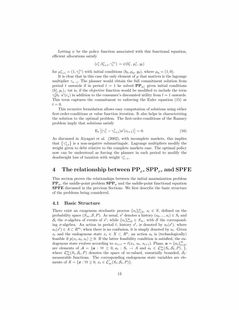
Letting ψ be the policy function associated with this functional equation,efficient allocations satisfy

(c∗t , b∗t+1, γ

1∗t ) = ψ(b∗t , µ

∗t , gt)

for µ∗t+1 = (1, γ1∗t ) with initial conditions (b0, µ0, g0), where µ0 = (1, 0).

It is clear that in this case the only element of µ that matters is the lagrangemultiplier γt−1. The planner would obtain the full commitment solution fromperiod t onwards if in period t = 1 he solved PPµ∗1

given initial conditions(b∗1, g1),; tat is, if the objective function would be modified to include the termγ1

0b1 u′(c1) in addition to the consumer’s discounted utility from t = 1 onwards.

This term captures the commitment to enforcing the Euler equation (15) att = 0.

This recursive formulation allows easy computation of solutions using eitherfirst-order-conditions or value function iteration. It also helps in characterizingthe solution to the optimal problem. The first-order-conditions of the Ramseyproblem imply that solutions satisfy

Et[(γ1t − γ1

t+1)u′(ct+1)]

= 0. (16)

As discussed in Aiyagari et al. (2002), with incomplete markets, this impliesthat

{γ∗1,t}

is a non-negative submartingale. Lagrange multipliers modify theweight given to debt relative to the complete markets case. The optimal policynow can be understood as forcing the planner in each period to modify thedeadweight loss of taxation with weight γ∗t−1.

4 The relationship between PPµ, SPPµ, and SPFE

This section proves the relationships between the initial maximization problemPPµ, the saddle-point problem SPPµ and the saddle-point functional equationSPFE discussed in the previous Sections. We first describe the basic structureof the problems being considered.

4.1 Basic Structure

There exist an exogenous stochastic process {st}∞t=0, st ∈ S, defined on theprobability space (S∞,S, P ). As usual, st denotes a history (s0, ..., st) ∈ St andSt the σ-algebra of events of st; while {st}∞t=0 ∈ S∞, with S the correspond-ing σ-algebra. An action in period t, history st, is denoted by at(st), whereat(st) ∈ A ⊂ Rm; when there is no confusion, it is simply denoted by at. Givenst and the endogenous state xt ∈ X ⊂ Rn, an action at is (technologically)feasible if p(xt, at, st) ≥ 0. If the latter feasibility condition is satisfied, the en-dogenous state evolves according to xt+1 = `(xt, at, st+1). Plans, a = {at}∞t=0,are elements of A = {a : ∀t ≥ 0, at : St → A and at ∈ Lm∞(St,St, P ), },where Lm∞(St,St, P ) denotes the space of m-valued, essentially bounded, St-measurable functions. The corresponding endogenous state variables are ele-ments of X = {x : ∀t ≥ 0, xt ∈ L

n

∞(St,St, P )}.

13

Given initial conditions (x, s), a plan a ∈ A and the corresponding x ∈ X ,the evaluation of such plan in PPµ is given by

f(x,µ.s)(a) = E0

k∑j=0

Nj∑t=0

βtµjhj0(xt, at, st)

We can describe the forward-looking constraints by defining g : A → Lk+1∞

coordinatewise as

g(a) jt = Et

Nj+1∑n=1

βnhj0(xt+n, at+n, st+n)

+ hj1(xt, at, st)

Given initial conditions (x, s), the corresponding feasible set of plans is then

B(x, s) = {a ∈ A : p(xt, at, st) ≥ 0, g(a) t ≥ 0, x ∈ X ,

xt+1 = `(xt, at, st+1) for all t ≥ 0, given (x0, s0) = (x, s)} .

Then PPµ can be written in compact form as

PPµ supa∈B(x,s)

f(x,µ.s)(a)

We denote solutions to this problem as a∗ and the corresponding sequenceof state variables x∗. When the solution exists we define the value function ofPPµ as

Vµ(x, s) = f(x,µ.s)(a∗) (17)

Similarly, we can also write SPPµ in a compact form, by defining

B′(x, s) = {a ∈ A : p(xt, at, st) ≥ 0, g(a) t+1 ≥ 0; x ∈ Xxt+1 = `(xt, at, st+1) for all t ≥ 0, given (x0, s0) = (x, s)} .

SPPµ infγ∈Rl

+

supa∈B′(x,s)

{f(x,µ,.s)(a) + γg(a)0

}Note that B′ only differs from B in that the forward-looking constraints inperiod zero g(a) 0 ≥ 0 are not included as a condition in the set B′, insteadthese constraints form part of the objective function of SPPµ.

4.2 Assumptions and existence of solutions to PPµ

We consider the following set of assumptions:

A1. st takes values on a set S ⊂ RK . {st}∞t=0 is a Markovian stochastic processdefined on the probability space (S∞,S, P ).

A2. (a) X ⊂ Rn and A is a closed subset of Rm. (b) The functions p :X ×A×S → R and ` : X ×A×S → X are measurable and continuous.

14

A3. Given (x, s),there exist constants B > 0 and ϕ ∈ (0, β−1), such that ifp(x, a, s) ≥ 0 and x′ = `(x, a, s′), then ‖a‖ ≤ B ‖x‖ and ‖x′‖ ≤ ϕ ‖x‖

A4. The functions hji (·, ·, s), i = 0, 1, j = 0, ..., l, are continuous and uniformlybounded, and β ∈ (0, 1).

A5. The function `(·, ·, s) is linear and the function p(·, ·, s) is concave. X andA are convex sets.

A6. The functions hji (·, ·, s), i = 0, 1, j = 0, ..., l, are concave.

A6s. In addition to A6, the functions hj0(x, ·, s), j = 0, ..., l, are strictly con-cave.

A7. For all (x, s), there exists a program {an}∞n=0 , with initial conditions (x, s),which satisfies the inequality constraints (4) and (5) with strict inequality.

Assumptions A1 and A2 are part of our basic structure, described in theprevious sub-section. These assumptions, together with A3-A4, are standardand we treat them as our basic assumptions. Assumptions A5-A7 are oftenmade but they are not satisfied in some interesting models; however, theseassumptions are only used in some of the results below. For example, theconcavity assumptions A5-A6 are not needed for many results, and assumptionA7 is a standard interiority assumption, only needed to guarantee the existenceof Lagrange multipliers.

The following proposition gives sufficient conditions for a maximum to existfor any µ. The aim is not to have the most general existence theorem14, butto stress that one can find fairly general conditions under which PPµ has asolution for any µ, which will be crucial in the discussion of how our approachcompares with that of Abreu Pearce and Stachetti, since this ensures that thecontinuation problem (namely PPϕ(µ,γ)) is well defined for any γ.

Proposition 1. Assume A1-A6 and that the set of possible exogenous statesS is countable. Fix (x, µ, s) ∈ X×Rl+1

+ ×S. Assume there exists a feasibleplan a ∈ B(x, s) such that f(µ,x,s)(a) > −∞. Then there exists a programa∗ which solves PPµ with initial conditions x0 = x, s0 = s.

Furthermore, if A6s is also satisfied then the solution is (almost sure) unique.

Proof: See Appendix.

4.3 The relationship between PPµ and SPPµ

The following result says that a solution to the maximum problem is also a solu-tion to the saddle point problem. It follows from standard theory of constrainedoptimization in linear vector spaces (see, for example, Luenberger (1969, Sec-tion 8.3, Theorem 1 and Corollary 1). As in the standard theory, convexity and

14For example, not requiring A6 or the countability of S, which will require additionalassumptions.

15

concavity assumptions (A5 to A6), as well as an interiority assumption (A7)are necessary in order to obtain the result.

Theorem 1 (PPµ =⇒ SPPµ). Assume A1-A7 and fix µ ∈ Rl+1+ . Let a∗ be

a solution to PPµ with initial conditions (x, s).There exists a γ∗ ∈ Rl+such that (a∗, γ∗) is a solution to SPPµ with initial conditions (x, s).

Furthermore, the value of SPPµ is the same as the value of PPµ, more pre-cisely

Vµ(x, s) = f(x,µ,.s)(a∗) + γ∗g(a∗)0 (18)

Proof: It is an immediate application of Theorem 1 (8.3) in Luenberger(1969), p. 217.

The following is a theorem on the sufficiency of a saddle point for a maximum.

Theorem 2 (SPPµ =⇒ PPµ). Given any (x, µ, s) ∈ X×Rl+1+ ×S, let (a∗, γ∗)

be a solution to SPPµ for initial conditions (x, s). Then a∗ is a solutionto PPµ for initial conditions (x, s).

Furthermore, the value of the two programs is the same and (18) holds.

Notice that Theorem 2 is a sufficiency theorem ‘almost free of assumptions.’All that is needed is the basic structure of section 4.1 defining the correspondinginfinite-dimensional optimization and saddle-point problems together with theassumption that a solution to SPPµ exists. Once these conditions are satisfiedassumptions A2 to A7 are not needed.

Proof: The following proof is an adaptation, to SPPµ, of a sufficiency theo-rem for Lagrangian saddle points (see, for example, Luenberger (1969),Theorem 8.4.2, p.221).

If (a∗, γ∗) solves SPPµ, minimality of γ∗ implies that, for every γ ≥ 0,

( γ∗ + γ) g(a∗)0 ≥ γ∗g(a∗)0;

therefore, g(a∗) 0 ≥ 0, but since a∗ ∈ B′(x, s), it follows that a∗ ∈ B(x, s);i.e. a∗ is a feasible program for PPµ. Furthermore, the minimality of γ∗

implies thatγ∗g(a∗)0 ≤ 0g(a∗)0 = 0

but since γ∗ ≥ 0 and g(a∗)0 ≥ 0, it follows that γ∗g(a∗)0 = 0. Now,suppose there exist a ∈ B(x, s) satisfying f(x,µ,s)(a) > f(x,µ,s)(a∗), then,since γ∗g(a)0 ≥ 0, it must be that

f(x,µ,s)(a) + γ∗g(a)0 > f(x,µ,s)(a∗) + γ∗g(a∗)0

which contradicts the maximality of a∗ for SPPµ.

Finally, using γ∗g(a∗)0 = 0, we have f(x,µ,s)(a∗) + γ∗g(a∗)0 = Vµ(x, s) �

16

4.4 The relationship between SPPµ, and SPFE

Recall that a function W : X×Rl+1+ ×S → R satisfies SPFE at (x, µ, s) when

W (x, µ, s) = minγ≥0

maxa∈A{µh0(x, a, s) + γh1(x, a, s) + β E [W (x′, µ′, s′)| s]}

(19)

s.t. x′ = `(x, a, s), p(x, a, s) ≥ 0 (20)and µ′ = ϕ(µ, γ). (21)

In (19) we have substituted inf sup by min max, implicitely assuming that asolution to the saddle point problem exists, in which case the value, W (x, µ,s), is uniquely determined15. In other words, the right side of SPFE is welldefined for all (x, µ, s) and W for which a saddle point exists.

We say that W satisfies SPFE if it satisfies SPFE at any possible state(x, µ, s) ∈ X × Rl+1

+ × S. Given W,we define the saddle-point policy correspon-dence (SP policy correspondence) Ψ : X ×Rl+1

+ × S → A×Rl+1+ by

ΨW (x, µ, s) ={

( a∗, γ∗) : a∗ ∈ arg maxa∈A, x′∈X

µh0(x, a, s) + γ∗h1(x, a, s) + β E [W (x′, µ∗′, s′)| s]

for µ∗′ = ϕ(µ, γ∗) and (20);γ∗ ∈ arg min

γ≥0µh0(x, a∗, s) + γh1(x, a∗, s) + β E [W (x∗′, µ′, s′)| s] ,

for x∗′ = `(x, a∗, s) and (21)}

If ΨW is single valued, we denote it by ψW , and we call it a saddle-point policyfunction (SP policy function).

We define the function W ∗(x, µ, s) ≡ Vµ(x, s). The following theorem saysthat W ∗ satisfies SPFE.

Theorem 3 (SPPµ =⇒ SPFE). Assume that SPPµ has a solution for any(x, µ, s) ∈ X × Rl+1

+ × S, then W ∗ satisfies SPFE. Furthermore, letting(a∗, γ∗) be a solution to SPPµ at (x, s), we have (a∗0, γ

∗) ∈ ΨW∗(x, µ, s).

As in Theorem 2, Theorem 3 is also a theorem ‘almost free of assumptions,’once the underlying structure and the existence of a well defined solution toSPPµ at all possible (x, µ, s) is assumed.

Proof: By theorem 2, we have that whenever SPPµ has a solution W ∗ is welldefined. Then, we first prove that, for any given (x, µ, s), if (a∗, γ∗) solvesSPPµ at (x, s) the following recursive equation is satisfied:

W ∗(x, µ, s) = µh0(x, a∗0, s)+γ∗h1(x, a∗0, s)+β E [W ∗(x∗1, ϕ(µ, γ∗), s′)| s](22)

15See Lemma 3A in Appendix B.

17

To prove ≤ in (22) we write

W ∗(x, µ, s) = f(x,µ,s)(a∗) + γ∗g(a∗)0= µh0(x, a∗0, s) + γ∗h1(x, a∗0, s)

+βE

l∑j=0

ϕj(µ, γ∗)Nj∑t=0

βt hj0(x∗t+1, a∗t+1, st+1) | s

= µh0(x, a∗0, s) + γ∗h1(x, a∗0, s) + βE

[f(x∗1 ,ϕ(µ, γ∗),s1)(σa

∗)| s]

≤ µh0(x, a∗0, s) + γ∗h1(x, a∗0, s) + βE[Vϕ(µ, γ∗)(x∗1, s1)| s

]= µh0(x, a∗0, s) + γ∗h1(x, a∗0, s) + βE [W ∗(x∗1, ϕ (µ, γ∗, s))| s]

where σa∗ is the original optimal sequence shifted one period; formally,letting the shift operator σ : St+1 → St be given by σ(st) = (s1, s2..., st),we define the St+1-measurable function σa∗t by σa∗t (s) ≡ a∗t+1(s). Thefirst equality follows from the definition of W ∗ and because Theorem 2guarantees (18), the second equality follows from the definition of f, g andsimple algebra, the third equality follows from the definitions of f , ϕ, anda∗. The weak inequality follows from the fact a∗ is a feasible solutionfor the problem PPϕ(µ, γ∗) with initial conditions (x∗1, s1) and that thisprogram achieves Vϕ(µ, γ∗)(x∗1, s1) at its maximum, and the last equalityfollows from Theorem 2 and (18).

To show ≥ (22) we construct a sequence a+ that consists of the optimalchoice for SPPµ for initial conditions (x, s) in the initial period, butsubsequently is followed by the optimal choices for PPϕ(µ, γ∗(x,µ,s)) forinitial conditions (x∗1, s1). To define a+ formally we explicitly denote by(a∗(x, µ, s), γ∗(x, µ, s)) a solution to SPPµ for given initial conditions(x, s) and we let

a+0 (x, µ, s) = a∗0(x, µ, s)a+t (x, µ, s) = σa∗t−1(x∗1, ϕ (µ, γ∗(x, µ, s), s) , s1)

for all (x, µ, s) and t ≥ 1. Also, we let x+ be the corresponding sequenceof state variables.

In what follows, we simplify again notation and we go back to denoting a∗t (x, µ, s)by a∗t , γ

∗(x, µ, s) by γ∗, and a+t (x, µ, s)(st) by a+

t ; then, we have:

W ∗(x, µ, s) = f(x,µ,s)(a∗) + γ∗g(a∗)0≥ f(x,µ,s)(a+) + γ∗g(a+)0= µh0(x, a+

0 , s) + γ∗h1(x, a+0 , s)

+βE

l∑j=0

ϕ(µ, γ∗)jNj∑t=0

βt hj0(x+t+1, a

+t+1, st+1) | s

= µh0(x, a∗0, s) + γ∗h1(x, a∗0, s)

+βE [W ∗(x∗1, ϕ (µ, γ∗) , s1)| s] ,

18

where the first equality has been argued before, the first inequality followsfrom the fact that a+(x, µ, s) is a feasible allocation in SPPµ for initialconditions (x, s) – but a∗(x, µ, s) is a solution of the max part to SPPµ at(x, s). The second equality just applies the definition of f and g, the lastequality follows because a+ is optimal for PPϕ(µ, γ∗(x,µ),s) given initialconditions (x∗1, s1) from period 1 onwards and because Theorem 2 insuresthat (18) holds.

Notice that for this step of the proof it is crucial that we use SPPµ in orderto obtain a recursive formulation. The first inequality above only worksbecause we are considering a saddle point problem. Indeed, the a+ se-quence (that reoptimizes in period t = 1) is feasible for SPPµ because thisproblem does not impose the forward looking constraints in t = 0. Thesequence a+ would not be feasible in the original problem PPµ, becauseby reoptimizing at period t = 1 the forward-looking constraints at t = 0would be typically violated.

This ends the proof of (22).

To show that W ∗ satisfies SPFE we now prove that the right side of SPFE iswell defined at W ∗ and that (a∗0, γ

∗) is a saddle point of the right side of(19) or, formally, that (a∗0, γ

∗) ∈ ΨW∗(x, µ, s).

We first prove that a∗0 solves the max part of the right side of SPFE. Given anya ∈ A, p(x, a, s) ≥ 0, letting a∗t (s

t) ≡ a∗t−1(`(x, a, s′), ϕ(µ, γ∗), s′)(σ(st))for t ≥ 1, the definition of a∗t , and (18) give the first equality in

µh0(x, a, s) + γ∗h1(x, a, s) + βE [W ∗(`(x, a, s′), ϕ(µ, γ∗), s′)| s]= µh0(x, a, s) + γ∗h1(x, a, s)

+βE

l∑j=0

ϕ(µ, γ∗)jNj∑t=0

βt hj0(x∗t+1, a∗t+1, st+1) | s

= f(x,µ,s)(a

∗) + γ∗g(a∗)0≤ f(x,µ,s)(a∗) + γ∗g(a∗)0= W ∗(x, µ, s)

the second equality follows by definition, and the inequality because (a∗, γ∗)solves the max part of SPPµ while the third equality follows from (18).Now we can combine this with (22) to obtain that for all feasible a ∈ A

µh0(x, a, s) + γ∗h1(x, a, s) + βE [W ∗(x∗1, ϕ(µ, γ∗), s′)| s]≤ µh0(x, a∗0, s) + γ∗h1(x, a∗0, s) + βE [W ∗(x∗1, ϕ(µ, γ∗), s′)| s]

implying that a∗0 solves the max part of the right side of the SPFE.

19

A similar argument shows that γ∗ solves the min part: for any γ ∈ Rl+1+ let

now

µh0(x, a∗0, s) + γh1(x, a∗0, s) + βE [W ∗(x∗1, ϕ(µ, γ), s′)| s]≥ µh0(x, a∗0, s) + γh1(x, a∗0, s) +

+βE

l∑j=0

ϕ(µ, γ)jNj∑t=0

βt hj0(x∗t+1, a∗t+1, st+1) | s

= f(x,µ,s)(a∗) + γ g(a∗)0≥ f(x,µ,s)(a∗) + γ∗ g(a∗)0= W ∗(x, µ, s)= µh0(x, a∗0, s) + γ∗h1(x, a∗0, s) + βE [W ∗(`(x, a∗0, s

′), ϕ(µ, γ∗), s′)| s]

where the inequality follows from the fact that shifting the policies oneperiod back of the plan a∗ is a feasible plan for the PPϕ(µ, eγ) problem withinitial conditions (x∗1, s

′) and that W ∗(x∗1, ϕ(µ, γ), s′) is the optimal valueof PPϕ(µ, eγ), the second inequality follows because (a∗, γ∗) is a saddlepoint of SPPµ and the equalities follow from definitions, Theorem 2 and(22).

Therefore γ∗ solves the min part of the right side of SPFE.

Therefore (a∗0, γ∗) is a saddle point of the right side of SPFE, this implies the

first equality in

minγ≥0

maxa∈A{µh0(x, a, s) + γh1(x, a, s) + β E [W ∗(x′, µ′, s′)| s]}

= µh0(x, a∗0, s) + γ∗h1(x, a∗0, s) + β E [W ∗(x∗1, ϕ(µ, γ∗), s′)| s]= W ∗(x, µ, s)

and the second equality comes, again, from (22). This proves that W ∗ satisfiesSPFE.�

The argument used in the proof of Theorem 3 can be iterated a finite numberof times to show the underlying recursive structure of the PPµ formulation. IfPPµ has a unique solution {a∗t }

∞t=0 at (x, s), then by Theorem 1 there is a SPPµ

at (x, s) with solution ({a∗t }∞t=0 , γ

∗), which in turn defines a PPϕ(µ, γ∗) prob-lem. As it has been seen in the proof of Theorem 3, {a∗t }

∞t=1 solves PPϕ(µ, γ∗)

at (`(x, a∗0, s), s1) and by Theorem 1 there is a γ∗1 such that ({a∗t }∞t=1 , γ

∗1)

solves SPPϕ(µ, γ∗) at (`(x, a∗0, s), s1). In turn, {a∗t }∞t=2 solves PPϕ(2)(µ, γ∗) at

(`(2)(x, a∗0, s), s1) where ϕ(2)(µ, γ∗) ≡ ϕ(ϕ(µ, γ∗), γ∗1, s1) and `(2)(x, a∗0, s) ≡`(`(x, a∗0, s), a

∗1, s1). Similarly, let ϕ(n+1)(µ, γ∗) ≡ ϕ(ϕ(n)(µ, γ∗), γ∗n, sn), then

by recursively applying the argument of the proof of Theorem 3 we obtain thefollowing result.

20

Corollary 3.1. (Recursivity of PPµ). If PPµ satisfies the assumptions ofTheorem 1 and has a unique solution {a∗t }

∞t=0 at (x, s), then, for any

(t, x∗t , st),{a∗t+j

}∞j=0

is the solution to PPϕ(t)(µ, γ∗) at (x∗t , st), where γ∗

is the minimizer of SPPµ at (x, s).

The value function has some interesting properties that we would like toemphasize. First, notice that

W ∗(x, µ, s) = f(x,µ,s)(a∗) + γ∗g(a∗)0= f(x,µ,s)(a∗)

= E0

l∑j=0

Nj∑t=0

βtµjhj0(x∗t , a∗t , st),

therefore, if {a∗t }∞t=0 at (x, s) is uniquely defined, then W ∗ has a unique repre-

sentation

W ∗(x, µ, s) =l∑

j=0

µjω∗j (x, µ, s)

= µω∗(x, µ, s)

where, for j = 0, ...k, ωj(x, µ, s) ≡ E0

∑∞t=0 β

thj0(x∗t , a∗t , st), and, for j = k +

1, ...l, ωj(x, µ, s) ≡ hj0(x∗0, a∗0, s0). Similarly, the value function of SPPϕ(µ, γ∗)

at (x∗1, s1), x∗1 = `(x, a∗0, s), satisfies

W ∗(x∗1, ϕ(µ, γ∗), s1) ≡ ϕ(µ, γ∗)ω∗(x∗1, ϕ(µ, γ∗), s1).

This representation not only has an interesting economic meaning – for example,as a ‘social welfare function,’ with varying weights, in problems with intertem-poral participation constraints – but is also very convenient analytically. Inparticular, this reprensentation shows16 that W ∗ is convex and homogenous ofdegree one in µ, with W ∗(x, 0, s) = 0, for all (x, s)17. In addition, the fol-lowing Corollary to Theorem 3 also shows that W ∗ satisfies what we call thesaddle-point inequality property SPI. Lemmas 1 and 2 below show how theseproperties are extended to general W functions satisfying SPFE.

A function W (x, µ, s) =∑lj=0 µ

jωj(x, µ, s) satisfies the saddle-point inequal-ity property SPI at (x, µ, s) if and only if there exist (a∗, γ∗) satisfying

µh0(x, a∗, s) + γh1(x, a∗, s) + β E [ϕ(µ, γ)ω(x∗′, ϕ(µ, γ∗), s′)| s]

≥ µh0(x, a∗, s) + γ∗h1(x, a∗, s) + β E [ϕ(µ, γ∗)ω(x∗′, ϕ(µ, γ∗), s′)| s] . (23)

≥ µh0(x, a, s) + γ∗h1(x, a, s) + β E [ϕ(µ, γ∗)ω(x′, ϕ(µ, γ∗), s′)| s] , (24)16See Lemma 2A in the Appendix B.17A function which is convex, homogeneous of degree one and finite at 0, is also called a

sublinear function (see Rockafellar, 1981, p.29).

21

for any γ ∈ Rl+1+ and ( a, x′) satisfying the technological constraints at (x, s);

that is, in SPI the multiplier minimization is taken in relation to the optimalcontinuation values.

Corollary 3.2. (SPPµ =⇒SPI). Let W ∗(x, µ, s) ≡ Vµ(x, s) be the value ofSPPµ at (x, s), for an arbitrary (x, µ, s), thenW ∗(x, µ, s) =

∑lj=0 µ

jω∗j (x, µ, s)satisfies SPI.

Proof: We only need to show that (23) is satisfied, but this is immediate fromthe following identities

f(x,µ,s)(a∗) = µh0(x, a∗0, s) + β E

k∑j=0

µjω∗j (x∗1, ϕ(µ, γ∗), s1)| s

γg(a∗)0 = γ [h1(x, a∗0, s) + β E [ω∗(x∗1, ϕ(µ, γ∗), s1)| s]] ,

and the definition of SPPµ at (x, s); that is, for any γ ∈ Rl+1+ ,

µh0(x, a∗, s) + γh1(x, a∗, s) + β E [ϕ(µ, γ)ω∗(x∗′, ϕ(µ, γ∗), s′)| s]= f(x,µ,s)(a∗) + γg(a∗)0≥ f(x,µ,s)(a∗) + γ∗g(a∗)0= µh0(x, a∗, s) + γ∗h1(x, a∗, s) + β E [ϕ(µ, γ∗)ω∗(x∗′, ϕ(µ, γ∗), s′)| s]

�

We now show that, under fairly general conditions, programs satisfyingSPFE are solutions to SPPµ at (x, s). More formally,

Theorem 4 (SPFE =⇒ SPPµ) Assume W , satisfying SPFE, is continuousin (x, µ) and convex and homogeneous of degree one in µ. If the SP policycorrespondence ΨW , associated withW , generates a solution (a∗,γ∗)(x,µ,s),where (a∗)(x,µ,s) is uniquely determined, then (a∗,γ∗)(x,µ,s) is also a so-lution to SPPµ at (x, s).

Notice that the assumptions onW are very general. In particular, ifW (x, µ, s)is the value function of SPPµ at (x, s) (i.e. W (x, µ, s) ≡ Vµ(x, s)) then (asLemma 2A in Appendix B shows) it is convex and homogeneous of degree onein µ and, if A2 - A5 are satisfied it is continuous and bounded in (x, µ).The only ‘stringent condition’ is that (a∗)(x,µ,s) must be uniquely determined,which is the case when W is concave in x and A6s is satisfied ( see Corollary4.1.).

Before proving these results, we show that, as we have seen for W ∗, convexand homogeneous functions W satisfying SPFE have some interesting proper-ties, which are used in the proof of Theorem 4. First, without loss of generality(see F2 and F3 in Appendix C), we can express the recursive equation (19) inthe form

µωd(x, µ, s) = µh0(x, a∗, s) + γ∗h1(x, a∗, s)

+β E[ϕ(µ, γ)ωd

′(x∗′, ϕ(µ, γ∗), s′)| s

], (25)

22

where µωd(x, µ, s) = W (x, µ, s), and the vectors ωd and ωd′are (partial) di-

rectional derivatives, in µ,of W (x, µ, s) and W (x∗′, ϕ(µ, γ∗), s′), respectively.Therefore, the SPFE saddle-point inequalities take the form

µh0(x, a∗, s) + γh1(x, a∗, s) + β E[ϕ(µ, γ)ωd

′(x∗′, ϕ(µ, γ), s′)| s

]≥ µh0(x, a∗, s) + γ∗h1(x, a∗, s) + β E

[ϕ(µ, γ∗)ωd

′(x∗′, ϕ(µ, γ∗), s′)| s

](26)

≥ µh0(x, a, s) + γ∗h1(x, a, s) + β E[ϕ(µ, γ∗)ωd

′(x′, ϕ(µ, γ∗), s′)| s

], (27)

for any γ ∈ Rl+1+ and ( a, x′) satisfying the technological constraints at (x, s).

Second, as we show in Lemma 1, there is an equivalence between this SPFEproperty and the saddle-point inequality property, SPI, which substitutes (26)for

µh0(x, a∗, s) + γh1(x, a∗, s) + β E[ϕ(µ, γ)ωd

′(x∗′, ϕ(µ, γ∗), s′)| s

]≥ µh0(x, a∗, s)+γ∗h1(x, a∗, s)+β E

[ϕ(µ, γ∗)ωd

′(x∗′, ϕ(µ, γ∗), s′)| s

]. (28)

Third, as we show in Lemma 2, if in addition (a∗,γ∗)(x,µ,s) is uniquelydetermined, then W is differentiable in µ. Alternatively, if W is not differentiablein µ′, then different choices of ωd

′can result in different solutions and the union

of all these different solutions are the solutions to the saddle point problem,given by (28) and (27).

Lemma 1 (SPI ⇐⇒ SPFE). If W (x, ·, s) is convex and homogeneous of de-gree one, then (26) is satisfied if and only if (28) is satisfied. Furthermore,the inequality (28) is satisfied if and only if the following conditions aresatisfied, for j = 0, ..., l,

hj1(x, a∗0, s) + β E[ωd′

j (x∗

1, µ∗1, s1)| s

]≥ 0 (29)

γ∗j[hj1(x, a∗0, s) + β E

[ωd′

j (x∗

1, µ∗1, s1)| s

]]= 0. (30)

Proof of Lemma 1: That SPI =⇒ SPFE follows from F4 (see Appendix C).With respect to W (x∗′, ϕ(µ, γ), s′), F4 takes the form:

ϕ(µ, γ)ωd′(x∗′, ϕ(µ, γ), s′) ≥ ϕ(µ, γ)ωd

′(x∗′, ϕ(µ, γ∗), s′);

therefore (28) together with this latter inequality results in the followinginequalities, which show that (26) is satisfied whenever (28) is satisfied:

µh0(x, a∗, s) + γh1(x, a∗, s) + β E[ϕ(µ, γ)ωd

′(x∗′, ϕ(µ, γ), s′)| s

]≥ µh0(x, a∗, s) + γh1(x, a∗, s) + β E

[ϕ(µ, γ)ωd

′(x∗′, ϕ(µ, γ∗), s′)| s

]≥ µh0(x, a∗, s) + γ∗h1(x, a∗, s) + β E

[ϕ(µ, γ∗)ωd

′(x∗′, ϕ(µ, γ∗), s′)| s

]23

To see that SPFE =⇒ SPI, let

G(x, a∗, s)(γ, µ) ≡ µh0(x, a∗, s)+γh1(x, a∗, s)+β E[ϕ(µ, γ)ωd

′(x∗′, ϕ(µ, γ), s′)| s

],

and

F(x, a∗, s)(γ, µ) ≡ µh0(x, a∗, s)+γh1(x, a∗, s)+β E[ϕ(µ, γ)ωd

′(x∗′, ϕ(µ, γ∗), s′)| s

],

Then (26) reduces toG(x, a∗, s)(γ, µ) ≥ G(x, a∗, s)(γ∗, µ) and (28) to F(x, a∗, s)(γ, µ) ≥F(x, a∗, s)(γ∗, µ). Since G(x, a∗, s)(γ∗, µ) = F(x, a∗, s)(γ∗, µ), the above in-equalities (??) show that, if f(x, a∗, s)(γ∗, µ) ∈ ∂γF(x, a∗, s)(γ∗, µ), for allγ ≥ 0, then

G(x, a∗, s)(γ, µ)−G(x, a∗, s)(γ∗, µ) ≥ F(x, a∗, s)(γ, µ)− F(x, a∗, s)(γ∗, µ)(γ − γ∗) f(x, a∗, s)(γ∗, µ);

that is, f(x, a∗, s)(γ∗, µ) ∈ ∂γG(x, a∗, s)(γ∗, µ).

Let g(x, a∗, s)(γ∗, µ) be an extreme point of ∂γG(x, a∗, s)(γ∗, µ), sinceG(x, a∗, s)(γ, µ)is homogenous of degree one in γ, by F2 ∃ γk −→ γ∗with G differentiableat γk and∇G(x, a∗, s)(yk, µ) −→ g(x, a∗, s)(γ∗, µ). By homogeneity of degreezero of ωd

′(x∗′, µ′, s′) with respect to µ′

∇G(x, a∗, s)(γk, µ) = h1(x, a∗(x, µ, s), s)+β E[ωd′(x∗′(x, µ, s), ϕ(µ, γk), s′)| s

].

Given the differentiability of ∇G(x, a∗, s)(yk, µ) at γk, continuity18 of ϕ and ωd′,

implies that

g(x, a∗, s)(γ∗, µ) = h1(x, a∗(x, µ, s), s)+β E[ωd′(x∗′(x, µ, s), ϕ(µ, γ∗), s′)| s

],

and, therefore, g(x, a∗, s)(γ∗, µ) ∈ ∂γF(x, a∗, s)(γ∗, µ) – in fact, it is also anextreme point of ∂γF(x, a∗, s)(γ∗, µ). This shows that ∂γF(x, a∗, s)(γ∗, µ) =∂γG(x, a∗, s)(γ∗, µ), which, in turn, implies the equivalence between (26)and (28).

Finally, the proof of the Kuhn-Tucker conditions is standard. First, necessityof (29) follows from the fact that γ∗ ≥ 0 is finite, which will not be thecase if, for some j = 0, ..., l,

hj1(x, a∗0, s) + β E[ωd′

j (x∗

1, µ∗1, s1)| s

]< 0.

To see necessity of (30), let γ∗j(i) = γ∗j , if j 6= i, and γ∗i(i) = 0, then (28)results in:

µh0(x, a∗, s) + γ∗(i)h1(x, a∗, s) + β E[ϕ(µ, γ∗(i))ω

d′(x∗′, ϕ(µ, γ∗), s′)| s]

18The continuity of ωd′, is given, for example, by Theorem 4F (& Corollary 4G) in Rock-

afellar (1981).

24

≥ µh0(x, a∗, s) + γ∗h1(x, a∗, s) + β E[ϕ(µ, γ∗)ωd

′(x∗′, ϕ(µ, γ∗), s′)| s

],

which, together with (29), implies that

0 ≥ γ∗j[hj1(x, a∗0, s) + β E

[ωd′

j (x∗

1, µ∗1, s1)| s

]]≥ 0.

To see, that (29) and (30) imply (28), suppose they are satisfied and thereexists a γ ≥ 0, for which (28) it is not, then it must be that

γ[h1(x, a∗0, s) + β E

[ωd′(x∗

1, µ∗1, s1)| s

]]< γ∗

[h1(x, a∗0, s) + β E

[ωd′(x∗

1, µ∗1, s1)| s

]]= 0,

which contradicts (29)�

Lemma 2. If (a∗,γ∗)(x,µ,s) is generated by ΨW (x, µ, s) and (a∗)(x,µ,s) is uniquelydefined then W (x∗t , µ

∗t , st) is differentiable with respect to µ∗t ; for every

(x∗t , µ∗t , st),with (x∗t , µ

∗t ) realized by19 (a∗,γ∗)(x,µ,s) .

Proof of Lemma 2: By (30) the recursive equation (25) simplifies to

µωd(x, µ, s) = µh0(x, a∗, s) + β E

k∑j=0

µjωd′

j (x∗′, µ+ γ∗), s′)| s

,

Assume, for the moment, that (a∗,γ∗)(x,µ,s) is uniquely determined. Byrecursive iteration, it follows that

µωd(x0, µ0, s0) = µh0(x0, a∗0, s0)

+β E0

k∑j=0

µj(hj0(x∗1, a

∗1, s1) + βωd

′′

j (x∗2, µ+ γ∗0 + γ∗1), s2))| s0

= µh0(x0, a

∗0, s0) + β E0

k∑j=0

µj∞∑t=1

βthj0(x∗t , a∗t , st)| s0

;

therefore, uniqueness of (a∗,γ∗)(x,µ,s) implies: i) ωd(x, µ, s) is uniquelydefined: ωd(x, µ, s) = ω(x, µ, s) ≡ ∇µW (x, µ, s); which, in turn, impliesthatW (x, ·, s) is differentiable, and ii) ωj(x, µ, s) = E0

∑∞t=0 β

thj0(x∗t , a∗(x∗t , µ

∗t , st), st),

for j = 0, . . . k (with (x∗0, µ∗0, s0) ≡ (x, µ, s), x∗t+1 = `(x∗t , a

∗(x∗t , µ∗t , st), st),

and µ∗t+1 = µ∗ + γ∗(x∗t , µ∗t , st)), and ωj(x, µ, s) = hj0(x, a∗(x, µ, s), s),

for j = k + 1 . . . l19That is, (x∗0, µ

∗0) ≡ (x, µ), x∗t+1 = `(x∗t , a

∗t , st+1) and µ∗t+1 = ϕ(µ∗t , γ

∗t ).

25

Given (a∗)(x,µ,s), suppose now(a∗, γ∗

)(x,µ,s)

is also generated by ΨW (x, µ, s).Both saddle-point paths must have the same value (see Lemma 3A inAppendix B); in particular, following the same recursive argument:

µωd(x0, µ0, s0) = µh0(x0, a∗0, s0) + β E

k∑j=0

µjωd′

j (x∗′, µ+ γ∗), s′)| s

= µh0(x0, a

∗0, s0) + β E0

k∑j=0

µj∞∑t=1

βthj0(x∗t , a∗t , st)| s0

,which proves the differentiablity of W with respect to µ, even when(γ∗)(x,µ,s) is not uniquely determined (i.e. there may be kinks in thePareto frontier)�

An immediate, and important, consequence of Lemma 2 is the followingresult:

Corollary: If (a∗)(x,µ,s) is uniquely defined by ΨW (x, µ, s), from any initialcondition (x, µ, s), then the following (recursive) equations are satisfied:

ωj(x, µ, s) = hj0(x, a∗(x, µ, s), s) + β E [ωj(x∗′(x, µ, s), µ∗′(x, µ, s), s′)| s] ,if j = 0, ..., k, and (31)

ωj(x, µ, s) = hj0(x, a∗(x, µ, s), s) if j = k + 1, ..., l. (32)

Furthermore, (a∗)(x,µ,s) is uniquely defined by ΨW (x, µ, s) wheneverW (·, µ, s)is concave and A6s is satisfied.

Notice that, in proving Lemma 2, uniqueness of the solution paths has im-plied uniqueness of the value function decomposition: W = µω. This uniquedecomposition has implied the recursive equations (31) and (31). Uniquenessof the value function decomposition is equivalent to the differentiability of thevalue function. In fact, once it has been established that the value function isdifferentiable, one can obtain equations (31) and (31) as a simple application ofthe Envelope Theorem. For example, equation (31) is just20:

∂jW (x, µ, s) = hj0(x, a∗(x, µ, s), s)+β E [∂jW (x∗′(x, µ, s), µ∗′(x, µ, s), s′)| s] .

We now turn to the proof of Theorem 4, where these recursive equations (31)and (31) play a key role.

Proof (Theorem 4): By Lemma 2, there is a unique representationW (x, µ, s) =µω(x, µ, s). To see that solutions of SPFE satisfy the participation con-straints of SPPµ, we use the first-order-conditions (29) and 30), as well

20We use the standard notation ∂jW (x, µ, s) ≡ ∂W (x,µ,s)∂µi

, and also ωj(x, µ, s) ≡∂jW (x, µ, s)

26

as the recursive equations of the forward-looking constraints (31) and 32)of the previous Corollary. As in the proof of Lemma 2, equation (31) canbe iterated to obtain

ωj(x, µ, s) = E0

[ ∞∑t=0

βthj0(x∗t , a∗t , st)| s

], if j = 0, ..., k. (33)

Following the same steps for any t > 0 and state (x∗t , µ∗t , st), equation(32)

and (33) together with the inequality (29) show that the intertemporalparticipation constraints in PPµ – and therefore in SPPµ – are satisfied;that is,

EtNj+1∑n=1

βn hj0(x∗t+n, a∗t+n, st+n) +hj1(x∗t , a

∗t , st) ≥ 0, ; t ≥ 0, j = 0, ..., l

(34)Now, to see that solutions of SPFE are, in fact, solutions of SPPµ

we argue by contradiction. Suppose there exist a program {at}∞t=0 , and{xt}∞t=0, x0 = x, xt+1 = `(xt, at, st+1), satisfying the constraints of SPPµ

with initial condition (x, s) and such that

µh0(x, a0, s) + γ∗h1(x, a0, s)

+ βE

k∑j=0

(µj + γ∗j

) ∞∑n=1

βt hj0(xt, at, st) +l∑

j=k+1

γ∗jhj0(x1, a1, s1)| s

> µh0(x, a∗0, s) + γ∗h1(x, a∗0, s)

+ βE

k∑j=0

(µj + γ∗j

) ∞∑n=1

βt hj0(x∗t , a∗t , st) +

l∑j=k+1

γ∗jhj0(x∗1, a∗1, s1)| s

.(35)

The following string of equalities and inequalities, which we explain at the

27

end, contradict this inequality,

µh0(x, a∗0, s) + γ∗0h1(x, a∗0, s)

+ βE

k∑j=0

(µj + γ∗j

) ∞∑n=1

βt hj0(x∗t , a∗t , st) +

l∑j=k+1

γ∗jhj0(x∗1, a∗1, s1)| s

= µh0(x, a∗0, s) + γ∗0h1(x, a∗0, s) + β E [µ∗1ω(x∗1, µ

∗1, s1)| s] (36)

≥ µh0(x, a0, s) + γ∗0h1(x, a0, s) + β E [µ∗1ω(x1, µ∗1, s1)| s] (37)

= µh0(x, a0, s) + γ∗0h1(x, a0, s)+ β E [µ∗1h0(x1, a

∗(x1, µ∗1, s1), s1) + γ∗(x1, µ

∗1, s1)h1(x1, a

∗(x1, µ∗1, s1), s1)

(38)

+ βµ∗′(x1, µ∗1, s1)ω(x∗′(x1, µ

∗1, s1), µ∗′(x1, µ

∗1, s1), s2)| s]

≥ µh0(x, a0, s) + γ∗0h1(x, a0, s)+ β E [µ∗1h0(x1, a1, s1) + γ∗(x1, µ

∗1, s1)h1(x1, a1, s1) (39)

+ βµ∗′(x1, µ∗1, s1)ω(x2, µ

∗′(x1, µ∗1, s1), s2)| s]

≥ µh0(x, a0, s) + γ∗0h1(x, a0, s)+ β E [µ∗1h0(x1, a1, s1) + γ∗(x1, µ

∗1, s1)h1(x1, a1, s1) + βµ∗′(x1, µ

∗1, s1)ω(x2, µ

∗1, s2)| s]

(40)

≥ µh0(x, a0, s) + γ∗0h1(x, a0, s)+ β E [µ∗1 [h0(x1, a1, s1) + βω(x2, µ

∗1, s2)] | s] (41)

= µh0(x, a0, s) + γ∗0h1(x, a0, s) + β E [µ∗1h0(x1, a1, s1)| s]+ β2 E [µ∗1h0(x2, a

∗(x2, µ∗1, s2), s2) + γ∗(x2, µ

∗1, s2)h1(x2, a

∗(x2, µ∗1, s2), s2)

(42)

+ βµ∗′(x2, µ∗1, s2)ω(x∗′(x2, µ

∗1, s2), µ∗′(x2, µ

∗1, s2), s2)| s]

≥ µh0(x, a0, s) + γ∗0h1(x, a0, s)

+ βE

k∑j=0

(µj + γ∗j

) ∞∑t=1

βt hj0(x,t at, st) +l∑

j=k+1

γ∗jhj0(x1, a1, s1)| s

(43)

Notice that the first equality (36) is just uses the value function decomposi-tion, the other two equalities (38) and (42) are simple expansions of the of thesaddle-point value paths (i.e., of (25)) and in these expansions equations (31)and (31) play a key role. Inequalities (37) and (39) follow from the maximalityproperty of SPFE. Inequalities (40) and (41) require explanation. Inequality(40) follows from one of the properties of convex and homogeneous of degreeone functions (i.e. F4: µω(µ) ≥ µω(µ), see Appendix), given that (40) is sim-ply µ∗′(x1, µ

∗1, s1)ω(x2, µ

∗′(x1, µ∗1, s1) ≥ µ∗′(x1, µ

∗1, s1)ω(x2, µ

∗1, s2). Inequal-

ity (41) follows from applying the slackness inequality (29), as well as equations(32) and (33) to the plan generated by SPFE in state (x2, µ

∗1, s2) (i.e. to

{a∗t (x2, µ∗1, s2)}∞t=2); these inequalities are needed to show that such plan satis-

fies the corresponding SPP constraints (34); that is,[hj1(x1, a1, s1) + βωj(x2, µ

∗1, s2)

]≥

28

0, j = 0, ..., l. Finally, since the equality (42) is simply the equality (38) after oneiteration, repeated iterations result in the last inequality (43), which contradicts(35).

It only remains to show that the inf part of SPP is also satisfied. Reasoningagain by contradiction, suppose there exist a γ ≥ 0 such that

µh0(x, a∗0, s) + γh1(x, a∗0, s)

+ βE

k∑j=0

(µj + γj

) ∞∑n=1

βt hj0(x∗t , a∗t , st) +

l∑j=k+1

γjhj0(x∗1, a∗1, s1)| s

< µh0(x, a∗0, s) + γ∗h1(x, a∗0, s)

+ βE

k∑j=0

(µj + γ∗j

) ∞∑n=1

βt hj0(x∗t , a∗t , st) +

l∑j=k+1

γ∗jhj0(x∗1, a∗1, s1)| s

.(44)

Using the value function decomposition representation, this inequality can alsobe expressed as

γ [h1(x, a∗(x, µ, s), s) + β E [ω(x∗′(x, µ, s), µ∗′(x, µ, s), s′)| s]]< γ∗(x, µ, s) [h1(x, a∗(x, µ, s), s) + β E [ωj(x∗′(x, µ, s), µ∗′(x, µ, s), s′)| s]] ,

but the first-order-conditions (29) and (30) require that (28) is satisfied, i.e.

γ [h1(x, a∗(x, µ, s), s) + β E [ω(x∗′(x, µ, s), µ∗′(x, µ, s), s′)| s]]≥ γ∗(x, µ, s) [h1(x, a∗(x, µ, s), s) + β E [ωj(x∗′(x, µ, s), µ∗′(x, µ, s), s′)| s]] = 0

which contradicts (44)�Corollary to Lemma 2 implies the following Corollary to Theorem 4:

Corollary 4.1. Assume W , satisfying SPFE, is continuous in (x, µ), convexand homogeneous of degree one in µ, concave in x and that A6s is satisfied.If (a∗,γ∗)(x,µ,s) is generated by ΨW (x, µ, s) then (a∗,γ∗)(x,µ,s) is also asolution to SPPµ at (x, s).

5 DSPP and the contraction mapping

In this Section we show how our main results –Theorems 3 and 4– can alsobe obtained by applying the Contraction Mapping Theorem to the DynamicSaddle-Point Problem, corresponding to SPFE. This Section provides moregeneral sufficient conditions to obtain a solution to the original problem PPµ

starting from SPFE. While these conditions are satisfied whenever the condi-tions of Theorem 4 are satisfied, they help to better understand the passageSPFE→PPµ and, in particular, they show how the standard method of valuefunction iteration extends to our saddle-point problems and, therefore, that com-puting solutions to our original PPµ does not require special computational

29

techniques. Furthermore, it also shows the interest of using the W = µω repre-sentation in computing recursive contracts (i.e. taking ω as the starting vectorvalued function) and how, in contrast with the ‘promise keeping’ approach tosolving contractual problems, ‘promised values’ are not part of the constraints,but an outcome of the recursive contract21.

We first define some spaces of “value” functions

Mb ={W : X ×Rl+1+ × S → R

i)W (·, ·, s) is continuous, and W (·, µ, s) bounded, when ‖µ‖ ≤ 1,ii)W (x, ·, s) is convex and homogeneous of degree one}

and

Mbc ={W ∈Mb andiii)W (·, µ, s) is concave}.

Mb is a space of continuous, bounded functions (in x), and convex and ho-mogenous of degree one (in µ)22, whileMbc is the subspace of concave functions(in x). Both spaces are normed vector spaces with the norm

‖W‖ = sup {|W (x, µ, s)| : ‖µ‖ ≤ 1, x ∈ X, s ∈ S} .We show in Appendix D (Lemma 6A) that they are complete metric spaces;therefore, suitable spaces for the Contraction Mapping Theorem.

Since, whenever W satisfies (ii) it can be represented as W (x, µ, s) =µω(x, ·, s) (see Lemma 4A), it is convenient to define the corresponding spacesof functions:

Mb ={ω : X ×Rl+1+ × S → Rl+1 s.t., for j = 0, ..., l,

i)ωj(·, ·, s) is continuous, and ωj(·, µ, s) bounded, when ‖µ‖ ≤ 1ii)ωj(x, ·, s) is convex and homogeneous of degree zero}

and

Mbc ={ω ∈Mb s.t., for j = 0, ..., l,iii)ωj(·, µ, s) is concave}.

Notice that ω ∈ M uniquely defines a function W ∈ M, given by W ≡ µω,but W ∈ M does not uniquely define a Rl+1 valued function ω ∈ M ; it doeswhen, in addition, W is differentiable in µ (see Appendix C)23.

As we have seen in Section 424, when W ∗(x, µ, s) = Vµ(x, s) is the valueof SPPµ, with initial conditions (x, s), then W ∗(x, µ, s) =

∑lj=0 µ

jω∗j (x, µ, s)

21We further discuss the ‘promise keeping’ approach in Section 6.22Without loss of generality, we could also require that W (x, 0, s) < ∞ and then replace

(ii) by W (x, ·, s) is sublinear (see footnote 12).23M denotes either Mb or Mbc.24See also Lemma 2A in Appendix B.

30

with W ∗ ∈Mb, whenever A2 - A4 are satisfied (and W ∗ ∈Mbc if in additionA5 - A6 are satisfied); furthermore, ω∗ ∈ M is unique whenever (a∗)(x,µ,s) isuniquely defined.

Given a function ω ∈M , and an initial condition (x, µ, s), we can define thefollowing Dynamic Saddle Point Problem:

DSPP

infγ≥0

supa{µh0(x, a, s) + γh1(x, a, s) + β E [µ′ω(x′, µ′, s′)| s]}

s.t. x′ = `(x, a, s), p(x, a, s) ≥ 0and µ′ = ϕ(µ, γ),

To guarantee that this problem has well defined solutions we make an interiorityassumption:

A7b. For any (x, s) ∈ X × S, there exists an a ∈ A, satisfying p(x, a, s) > 0,such that, for any µ′ ∈ Rl+1

+ , ‖µ′‖ < +∞, and j = 0, ..., l : hj1(x, a, s) +βE[ωj(`(x, a, s′), µ′, s′)| s

]> 0.

Notice that A7b is satisfied, whenever A7 is satisfied and µ′ω(`(x, a, s′), µ′, s′)is the value function of SPP(`(x,ea, s′),µ′,s′). In general, A7b is not a restrictiveassumption in the class of possible value functions if the original problem hasinterior solutions. Nevertheless, an assumption, such as A7b is needed whenone takes DSPP(x,µ,s) as the starting problem. This is a relatively standardmin max problem, except for the dependency of ω on ϕ(µ, γ). The followingproposition shows that it has a solution. Obviously, solutions to DSPP(x,µ,s)

satisfy SPFE. . An immediate consequence of A7b, is the following lemma:

Lemma 3. Assume A4 and A7b and let ω ∈Mb. There exist a B > 0, suchthat if (a∗(x, µ, s), γ∗(x, µ, s)) is a solution to DSPP at (x, µ, s), then‖γ∗(x, µ, s)‖ ≤ B ‖µ‖.

Proof: Denote by (a∗, γ∗) ≡ (a∗(x, µ, s), γ∗(x, µ, s)) the solution to DSPP at(x, µ, s), and let a be the interior solution of A7b, then

µh0(x, a∗, s) + γ∗h1(x, a∗, s) + β E [µ′ω(`(x, a∗, s), ϕ(µ, γ∗), s′)| s]

= µh0(x, a∗, s) + β E

k∑j=0

µjωj(`(x, a∗, s), ϕ(µ, γ∗), s′)| s

+ γ∗ [h1(x, a∗, s) + β E [ω(`(x, a∗, s), ϕ(µ, γ∗), s′)| s]]

= µh0(x, a∗, s) + β E

k∑j=0

µjωj(`(x, a∗, s), ϕ(µ, γ∗), s′)| s

≥ µh0(x, a, s) + β E

k∑j=0

µjωj(`(x, a, s), ϕ(µ, γ∗), s′)| s

+ γ∗ [h1(x, a, s) + β E [ω(`(x, a, s), ϕ(µ, γ∗), s′)| s]]

31

By assumption,

(µ/ ‖µ‖)h0(x, a∗, s)+β E

k∑j=0

(µj/ ‖µ‖)ωj(`(x, a∗, s), ϕ((µ/ ‖µ‖), (γ∗/ ‖µ‖)), s′)| s

is uniformly bounded ( A4 and ω ∈Mb imply that there is uniform boundfor the max value), while if (γ∗j/ ‖µ‖) > 0 then

(γ∗j/ ‖µ‖)[hj1(x, a, s) + βE [ωj(`(x, a, s), ϕ((µ/ ‖µ‖), (γ∗/ ‖µ‖)), s′)| s]

]> 0;

therefore, there must be a B > 0 such that ‖γ∗‖ ≤ B ‖µ‖�

Proposition 2. Let ω ∈ Mbc and assume A1-A6 and A7b. There exists(a∗, γ∗) that solves DSPP(x,µ,s). Furthermore if A6s is assumed, thena∗(x, µ, s) is uniquely determined.

Proof: It is a relatively standard proof of existence of an equilibrium, based ona fixed point argument; see Appendix D.

The following Corollary to Theorem 3, is a simple restatement of the theoremin terms of the Dynamic Saddle Point Problem

Corollary 3.3. (SPPµ(x, s) =⇒ DSPP(x,µ,s) ). Assume that SPPµ at (x, s)has a solution (a∗, γ∗) with value Vµ(x, s) =

∑lj=0 µ

jω∗j (x, µ, s), then(a∗0, γ

∗) solves DSPP(x,µ,s).

When DSPP(x,µ,s) has a solution, it defines a SPFE operator T ∗ :M−→M given by

(T ∗W )(x, µ, s) = minγ≥0

maxa{µh0(x, a, s) + γh1(x, a, s) + β E [W (x′, µ′, s′)| s]}

s.t. x′ = `(x, a, s), p(x, a, s) ≥ 0and µ′ = ϕ(µ, γ),

When W ≡ µω, with ω ∈ M , and DSPP(x,µ,s) uniquely defines the valueshj0(x, a∗(x, µ, s), s), j = 0, ..., l, then T ∗ defines a mapping, T : M −→ M ,given by

(Tωj)(x, µ, s) = hj0(x, a∗(x, µ, s), s)+β E [ωj(x∗′(x, µ, s), µ∗′(x, µ, s), s′)| s] ,(45)

if j = 0, ..., k, and

(Tωj)(x, µ, s) = hj0(x, a∗(x, µ, s), s), if j = k + 1, ..., l. (46)

Two remarks are in order. First, as already said, notice that (Tωj) correspondto the ‘promise keeping’ approach to solving contractual problems but in our

32

approach (Tωj) is not a constraint: it is an outcome. Second, a fixed pointof T ∗ does not imply a fixed point of T when ‘the planner’ is indifferent to Treallocations (e.g. µi = µj , µi(Tωi)+ µj(Tωj) = constant) resulting in multiple(indeterminate) continuation values (for i and j)25

Proposition 3. Assume DSPP has a solution, for any ω ∈ M and (x, µ, s),then T ∗ : M → M is a well defined contraction mapping. Let W ∗ =T ∗(W ∗) and W ∗ = µω∗, if in addition the solutions a∗(x, µ, s) to DSPPare unique, then ω∗ = T (ω∗) is unique.

Proof: The first part follows from showing that Blackwell’s sufficiency condi-tions for a contraction are satisfied for T ∗ (see Lemmas 7A to 10A inAppendix D), the second part from the definition of T .

Our last Theorem, Theorem 5, wraps up our sufficiency results and is, infact, a Corollary to Theorem 4. It shows how, starting from a Dynamic Saddle-Point Problem and a corresponding well defined Contraction Mapping resultingin a unique value function, one obtains the solution to our original problemPPµ. The previous Propositions 2 and 3 provide conditions guaranteeing thatthe assumptions of Theorem 5, regarding T , are satisfied.

Theorem 5 (DSPP(x,µ,s) =⇒ SPPµ(x, s)). Assume T : M →M has a uniquefixed point ω∗. Then the value function W ∗(µ, x, s) = µω∗(x, µ, s) is thevalue of SPPµ at (x, s) and the solutions of DSPP define a saddle-pointcorrespondenceΨ, such that if (a∗,γ∗) is generated by Ψ from (x, µ, s),then (a∗,γ∗) solves SPPµ at (x, s) and a∗ is the unique solution to PPµ

at (x, s).

Proof: By assumption SPFE is satisfied. The proof of Theorem 4 is basedon having a unique representation W ∗(µ, x, s) = µω∗(x, µ, s) which, inthat proof, is given by Lemma 2. In Theorem 5 such a unique represen-tation is assumed, which implicitly also means to assume that the valueshj0(x, a∗(x, µ, s), s) j = 0, ..., l are uniquely determined, which in fact isall what is needed in the proof of Theorem 4.

6 Related work

Precedents of our approach can be found in Epple, Hansen and Roberds (1985),Sargent (1987) and Levine and Currie (1987), who introduced lagrange mul-tipliers as co-state variables in linear-quadratic Ramsey problems. Similarly,recent studies of optimal monetary policy in sticky price models have includedlagrange multipliers as co-states. Often, the reason given for including thesepast multipliers as co-states is the observation that past multipliers appear in

25Messner and Pavoni’s ‘counterexample’ is one of these cases of ‘flats in the Pareto frontier’,when one only considers the T ∗ map and not the T map; see Marimon, Messner and Pavoni(2010).

33

the first-order-conditions of the Ramsey problem. Our work provides a formalproof that, with standard assumptions, co-state past multipliers deliver the op-timal solution in a general framework, encompassing a larger class of modelswith forward-looking constraints.

The pioneer work of Abreu, et al. (1990) -APS, from now on,- character-izing sub-game perfect equilibria, shows that past histories can be summarizedin terms of promised utilities. Earlier related work was by Green (1987) andThomas and Worral (1988). This approach has been widely used in macroe-conomics26. Some applications are by Kocherlakota (1995) in a model withparticipation constraints, Cronshaw and Luenberger (1994) in a dynamic game.Also, as in the earlier work Kydland and Prescott (1980), Chang (1998) andPhelan and Stacchetti (1999) study Ramsey equilibria using promised marginalutility as a state variable, and they note the analogy of their approach withAPS’s.

Both APS and our approach have in common that, starting from non-recursive problems, allow to obtain optimal solutions (obviously, the same solu-tions) where forward-looking constraints have a recursive structure. In relativelysimple problems (e.g., convex problems of full information and low dimension-ality, in terms of state variables and number of forward-looking constraints) thetwo approaches can be seen as mirrors of each other. Nevertheless, there is aconceptual difference which sets these two approaches further apart as morecomplex problems are analyzed: our state (including the co-state µ) is prede-termined, while promised-utilities – as co-state variables – are not; furthermore,in the APS approach, in taking future promised-utilities as choice variables,the recursive structure of forward-looking constraints must be taken as ‘promisekeeping’ constraints, while in our approach we obtain this recursive structureas a result (see, Subsection 2.1)27.

As it is well known promised utilities in the APS approach have to be re-stricted to lie in a set where the continuation problem is well defined, otherwisealgorithmic computations break down. The set of feasible promised utilitiesis not known beforehand, it can only be characterized numerically, often lead-ing to very complicated calculations. Whenever there are several natural statevariables the set of feasible promised utilities is a function of the natural statevariables and the problem of finding the set of feasible utilities is daunting.Considerable progress has been made either by improving algorithms or by re-defining the problem at hand28, but the issue of constraining promised utilities(or marginal utilities in a Ramsey problem) is always present.

One key advantage of our approach is that the continuation problem is givenby PPµ′ , and it is easy to find standard assumptions guaranteeing that thisproblem has a solution for any co-state µ′ ≥ 0; in fact, the set of feasible co-states is known beforehand, it is simply the positive orthant. The difficulties

26Ljungqvist and Sargent (2000) provides an excellent introduction, and reference, to mostof this recent work.

27We only provide a summary discussion of the contrast between both approaches, seeMarcet (2008) for more details.

28See, for example, Abraham and Pavoni (2005) or Judd, Yeltekin and Conklin (2003).

34

associated with computing a set of co-states for which the continuation problemis well defined are absent.

A second advantage lies in the dimensionality of the decision vector. In theAPS approach the planner has to decide at t the utility promised at all possiblestates in t+ 1. If the underlying exogenous state variable can take Ns possiblevalues the planner has to decide on at least Ns controls at t. Most applications ofAPS constrain themselves to assuming that the exogenous variable is binomial(say, it can be ”high” or ”low”), but if exogenous variables can take many valuesa high-dimensional decision vector has to be solved for. Again, there are waysof dealing with this, but it is no doubt an added difficulty. By contrast, in ourapproach the dimensionality of the decision variable is independent of Ns.

An additional issue is that the initial conditions for the state variables in ourapproach are given from the outset, namely µ0 = 1 and µj = 0 for j ≥ 1, whilein the promised utility approach the promised utility in the first period has tobe solved for separately. It is well known that for this it is needed that thePareto frontier is downward slopping, otherwise the computations can becomevery cumbersome.29

Finally, an interesting -but not exclusive- feature of our approach is that theevolution of µ often helps to directly characterize the behavior of the model. Forexample, in models with participation constraints the µ’s allow to interpret thebehavior of the model as changing the Pareto weights sequentially dependingon how binding the participation constraints become. In Ramsey type modelsthe behavior of the µ’s is associated with the commitment technology and therole that budget constraints play in the objective function of the planner. Wehave discussed these interpretations in Section 3. Also, our approach facilitatesto identify cases where despite the presence of forward-looking constraints theco-state variables do not need to be introduced in the model.30

The APS approach has some strengths over our approach. For example, itallows for the characterization of all feasible paths (not only the constrained-efficient) and it naturally applies to models with private information or modelswith multiple solutions. However, these initial advantages are also being over-come. Sleet and Yeltekin (2010) and Mele (2010) have extended our approachto address moral hazard problems. In problems with multiple (locally unique)solutions, it is also possible to find other feasible paths using our approachby changing the objective function. However, as the example of Messner andPavoni (2004) shows, there are problems where optimal paths are bound tohave a continuum of solutions (i.e. when the constrained-efficient Pareto fron-tier has flats). We have maintained the assumption of (local) uniqueness inthis paper; nevertheless, Marimon, Messner and Pavoni (2011) have recently

29Even with two agents and a downward slopping Pareto frontier, as in Kocherlakota (1996),one may be interested in finding the efficient allocation that ex-ante gives the same utility toboth agents. While this is trivial with our approach (just give the same initial weights in thePP problem), becomes very tricky with the APS approach since the ‘right promise’ must bemade to determine the initial conditions.

30This can be the case, for example, in Cooley, Quadrini and Marimon (2004) and Anag-nostopoulos, Carceles-Poveda and Marcet (2011).

35

shown that there is a natural extension of our approach to solve problems withnon-uniqueness 31.

Many applications of our approach can be found in the literature, althoughit is beyond the scope of this paper to discuss them in detail. This seems to betestimony of the convenience of using our approach, specially in the presenceof intertemporal participation constraints with natural state variables such ascapital (as in Subsection 3.1) or first-order Euler equation constraints with bondsas natural state (as in Subsection 3.2).

Perhaps most interesting is that the approach here can be used as an in-termediate step in solving models that go beyond the pure formulation of PP.For example, a second generation of models considers endogenous participationconstraints, as in the non-market exclusion models of Cooley et al. (2004), Ma-rimon and Quadrini (2011), and Ferrero and Marcet (2005). In these modelsthe functions h that appear in the incentive constraints are endogenous, theydepend on the optimal or equilibrium solution, and the approach of this paperis often used as an intermediate step, defining the underlying contracts. Thisallows the study of problems where the outside option is determined in equili-brum as in models of debt renegotiation and long-term contracts. Furthermore,the work of Debortoli and Nunes (2010) extends our approach to study modelsof partial commitment and political economy, and the work of Marimon andRendhal (2011) extend is to study models where agents can behave strategi-cally with respect to their participation constraints, as in dynamic bargainingproblems.

7 Concluding remarks

We have shown that a large class of problems with implementability constraintscan be analysed using an equivalent recursive saddle-point problem. This saddle-point problem obeys a saddle point functional equation, which is a version ofthe Bellman equation. This approach works for a very large class of modelswith incentive constraints: intertemporal enforcement constraint, intertemporalEuler equations in optimal policy policy or regulation design, etc. This meansthat a unified framework can be provided to analyse all these models. The keyfeature of our approach is that instead of having to write optimal contractsas history-dependent contracts one can write them as a stationary function ofthe standard state variables together with additional co-state variables. Theseco-state variables are – recursively – obtained from the Lagrange multipliers as-sociated with the intertemporal incentive constraints, starting from pre-specifiedinitial conditions. This simple representation also provides economic insight intothe analysis of various contractual problems; for example, with intertemporal

31Marimon, Messner and Pavoni (2011) show how the results presented here can be appliedwhen the co-state is extended with the ‘last non-negative multiplier’. Cole and Kubler (2010)also provide a solution for the non-uniqueness case. Their approach involves a mix of ourapproach and of the APS approach; they provide a solution for the two-agent case withintertemporal participation constraints.

36

participation constraints it shows how the (Bethamite) social planner changesthe weights assigned to different agents in order to keep them within the socialcontract; in Ramsey optimal problems it shows the cost of commitment to thebenevolent government.

We have provided here the first complete account of the basic theory of re-cursive contracts. Nevertheless, we had already expounded most of the elementsof the theory in our previous work (in particular, Marcet and Marimon (1988& 1999)), which has allowed others to built on it. Many applications are al-ready found in the literature, showing the convenience of our approach, speciallywhen natural state variables are present. Useful extensions are already availableencompassing a larger set of problems than the ones considered here.

37

8 Authors’ Affiliations

Albert Marcet, London School of Economics and CEP,E-mail: a.marcet@lse.ac.uk

andRamon Marimon, European University Institute and Universitat Pompeu

Fabra - BarcelonaGSE,Via delle Fontanelle 20, I-50014 San Domenico di Fiesole, Italy;

Telephone: +39-055-4685809, Fax: +39-055-4685894,E-mail: ramon.marimon@eui.eu

38

APPENDIX

Appendix A (Proof of Proposition 1)The proof of Proposition 1 relies on the following result:

Lemma 1A. Assume A1-A6 and that S is countable, then

i) B(x, s) is non-empty, convex, bounded and σ(L∞, L1) closed; therefore it isσ(L∞, L1) compact

ii) Given d ∈ R, the set{a ∈ A : f(x,µ,s)(a) ≥ d

}is convex and σ(L∞, L1)

closed

The proof of Lemma 1A builds on three theorems. First, the Urysohnmetrization theorem stating that regular topological spaces with a count-able base are metrizable32. Second, the Mackey-Arens theorem statingthat different topologies consistent with the same duality share the sameclosed convex sets; in our case, the duality is (L∞, L1) and the weak-est and the strongest topology consistent with such duality; namely, theweak-star, σ(L∞, L1) and the Mackey τ(L∞, L1) . Third, the Alaoglutheorem stating that norm bounded σ(L∞, L1) closed subsets of L∞ areσ(L∞, L1) compact33.

Proof:

Assumptions A2, and A4 - A6 imply that B(x, s) is convex, and closed underpointwise convergence. Since, by assumption S is countable, Urysohnmetrization theorem guarantees that B(x, s) is, in fact, σ(L∞, L1) closed.Assumptions A3 and A4 imply that B(x, s) is bounded in the ‖·‖β∞ normas needed for compactness, according to the Alaoglu theorem.

Assumptions A5 and A6 imply that B(x, s) and the upper contour sets {a ∈ A : fµ(a) ≥ d} ,are convex and, together with the previous assumptions (A2, and A4),Mackey closed and, therefore, σ(L∞, L1) closed34�

Proof of Proposition 1: As in Bewley (1991), the central element of the prooffollows from the Hausdorff maximal principle and an application of thefinite intersection property35. Let Pd =

{a ∈ B(x, s) : f(x,µ.s)(a) ≥ d

},

32See Dunford and Schwartz (1957) p. 24. in our case the metric we use is given by

ρβ∞(a, b) =

∞Xn=0

βn supsn∈Sn

| an(s)− bn(s) | .

33See Schaefer (1966) p. 130 and p. 84, respectively.34See Bewley (1972) for a proof of the Mackey continuity expected utility, without assuming

S being countable.35See, Kelley (1955) p. 33-34. for the Hausdorff principle and the Minimal principle, and

p. 136 for the theorem stating that ”a set is compact if and only if every family of closed setswhich has a the finite intersection property has a non-void intersection.”

39

then by Lemma 1A , Pd is σ(L∞, L1) closed. By the interiority assumptionof Proposition 1, for d low enough, it is non-empty. In fact, we can considerthe family of sets {Pd : d ∈ D} for which Pd 6= ∅, where D ⊂ R. The setsPd are ordered by inclusion; in fact, if d′ > d then Pd′ ⊂ Pd and every finitecollection of them has a non-empty intersection (i.e., {Pd : d ∈ D} satisfiesthe finite intersection property), but then by compactness of B(x, s) anyfamily of subsets of {Pd : d ∈ D} -say, {Pd : d ∈ B ⊂ D}- has a non-emptyintersection and, by inclusion, there is Pbd = ∩{Pd : d ∈ B ⊂ D} 6= ∅. Inparticular, there is Pd∗ = ∩{Pd : d ∈ D} 6= ∅ which -as the the minimalprinciple states- is a minimal member of the family {Pd : d ∈ D}. It fol-lows that if a∗ ∈ Pd∗ then f(x,µ.s)(a∗) ≥ f(x,µ.s)(a) for any a ∈ B(x, s).Furthermore, if strictly concavity is assumed then Pd∗ must be a single-ton, otherwise convex combinations of elements of Pd∗ will form a properclosed subset of Pd∗ contradicting its minimality�

Appendix B (Some Properties of W ∗)

Lemma 2A. Let W ∗(x, µ, s) ≡ Vµ(x, s) be the value of SPPµ at (x, s), for anarbitrary (x, µ, s), then

i) W ∗(x, ·, s) is convex and homogeneous of degree one;

ii) if A2- A4 are satisfied W ∗(·, µ, s) is continuous and uniformly bounded,and

iii) if A5 and A6 are satisfied W ∗(·, µ, s) is concave.

Proof: i) follows from the fact that, for any λ > 0, f(x,λµ.s)(a) = λf(x,µ.s)(a).To see this, let (γ∗,a∗) satisfy SFPE, i.e.

f(x,µ.s)(a∗) + γg(a∗)0≥ f(x,µ.s)(a∗) + γ∗g(a∗)0≥ f(x,µ.s)(a) + γ∗g(a)0,

for any γ ∈ Rl+1+ and a ∈ B′(x, s). Then (λγ∗,a∗) satisfies

f(x,λµ.s)(a∗) + γg(a∗)0≥ f(x,λµ.s)(a∗) + λγ∗g(a∗)0≥ f(x,λµ.s)(a) + λγ∗g(a)0,

for any γ ∈ Rl+1+ and a ∈ B′(x, s). ii) and iii) are straightforward; in par-

ticular, ii) follows from applying the Theorem of the Maximum (Stokey,Lucas and Prescott,1989, Theorem 3.6) iii) follows from the fact that theconstraint sets are convex and the objective function concave.�

Lemma 3A: If the inf sup problem, SPFE at (x, µ, s), has a solution thenthe value of this solution is unique.

40

Proof: It is a standard argument: consider two solutions to the right sideof SPFE at (x, µ, s), (a, γ) and (a, γ), then repeated application of thesaddle-point condition implies:

µh0(x, a, s) + γh1(x, a, s) + βE [W ∗(`(x, a, s′), ϕ(µ, γ), s′)| s]≥ µh0(x, a, s) + γh1(x, a, s) + βE [W ∗(`(x, a, s′), ϕ(µ, γ), s′)| s]≥ µh0(x, a, s) + γh1(x, a, s) + βE [W ∗(`(x, a, s′), ϕ(µ, γ), s′)| s]≥ µh0(x, a, s) + γh1(x, a, s) + βE [W ∗(`(x, a, s′), ϕ(µ, γ), s′)| s]≥ µh0(x, a, s) + γh1(x, a, s) + βE [W ∗(`(x, a, s′), ϕ(µ, γ), s′)| s]

therefore the value of the objective at both (a, γ) and (a, γ) coincides �

Appendix C (Some Properties of convex homogeneous functions)

To simplify the exposition of these properties let F : Rm+ → R continuous,convex and homogeneous of degree one. The subgradient set of F at y,denoted ∂F (y), is given by

∂F (y) ={z ∈ Rm | F (y′) ≥ F (y) + (y′ − y)z for all y′ ∈ Rm+

}.

The following facts, regarding F , are used in proving Lemmas 1 and 2:

F1. If F is convex, then it is differentiable at y if, and only if, ∂F (y) consists ofa single vector; i.e. ∂F (y) = {∇F (y)} , where ∇F (y) is called the gradientof F at y.

F2. If F is convex and finite in a neighborhood of y, then ∂F (y) is the convexhull of the compact set

{z ∈ Rm | ∃ yk −→ y with F differentiable at yk and ∇F (yk) −→ z} .

F3. Lemma 4A (Euler’s formula). If F is convex and homogeneous of de-gree one and z ∈ ∂F (y) then F (y) = yz.

F4. Lemma 5A. If F is convex and homogeneous of degree one, for any pair(f, f), if fd(y) ∈ ∂F (y) and fd(y) ∈ ∂F (y), then yfd(y) ≥ yfd(y).

F1 is a basic result on differentiability of convex functions (see, Rockafellar,1981, Theorem 4F, or 1970, Theorem 25.1). F2 is a very convenient charac-terization of the subgradient set of a convex function (see Rockafellar, 1981,Theorem 4D, or 1970, Theorem 25.6). We now provide a proof of the last twofacts.

Proof of Lemma 4A: Let z ∈ ∂F (y), then for any λ > 0, F (λy) − F (y) ≥(λy − y)z, and, by homogeneity of degree one: (λ − 1)F (y) ≥ (λ − 1)yz.If λ > 1 this weak inequality results in: F (y) ≥ yz; while if λ ∈ (0, 1) inF (y) ≤ yz�36

36Notice that this does not imply that F is linear, which requires that F (−y) = −F (y).

41

Proof of Lemma 5A: To see F4 notice that if fd(y) ∈ ∂F (y) and fd(y) ∈∂F (y), by convexity, homogeneity of degree one, and Euler’s formula:F (y) = yfd(y) and

F (y) ≥ F (y) + (y − y)fd(y)= yfd(y) + yfd(y)− yfd(y) = yfd(y).

Appendix D (Proof of Propositions 2 and 3)

Proof of Proposition 2: Given the assumptions of Proposition 2, for any(x, µ, s), and γ ∈ Rl+1

+ , let

F(x,µ,s)(γ) = arg supa

µh0(x, a, s) + β E

k∑j=0

µjωj(x′, µ′, s′)| s

s.t. x′ = `(x, a, s), p(x, a, s) ≥ 0

and µ′ = ϕ(µ, γ),

and hj1(x, a, s) + βE[ωj(x′, µ′, s′)| s

]≥ 0, j = 0, ..., l (47)

Since this is a standard maximization problem of a continuous function ona compact set, there is a solution a∗(x, µ, s; γ) ∈ F(x,µ,s)(γ). Furthermore,given that the constraint set is convex and has a non-empty interior (byA2 and A7b), there is an associated multiplier vector; let γ∗j(x, µ, s; γ)be the multiplier corresponding to (47), for j. In particular, by Lemma 3,γ∗(x, µ, s; γ) ∈ G(x,µ,s)(a∗), where

G(x,µ,s)(a) = arg inf{γ≥0:‖γ‖≤B‖µ‖}

{µh0(x, a, s) + γh1(x, a, s) + β E [ϕ(µ, γ)ω(x′, ϕ(µ, γ), s′)| s]}

s.t. x′ = `(x, a, s), p(x, a, s) ≥ 0

The rest of the proof is a trivial application of the Theorem of the Maxi-mum (e.g. Stokey et al. (1989), p. 62) and of Kakutani’s Fixed Point The-orem (e.g. Mas-Colell et al. (1995), p.953). First notice that µh0(x, a, s)+β E

[∑kj=0 µ

jωj(x′, µ′, s′)| s]

is continuous in a and, by A2, A4 and thedefinition of Mbc, G

∗(x,µ,s)(·) is also continuous. Second, let A(x, s) ≡

{a ∈ A : p(x, a, s) ≥ 0}, by A2 and A3 A(x; s) is compact and by A5 isconvex, while Ψ(µ) ≡ {γ ≥ 0 : ‖γ‖ ≤ B ‖µ‖} is trivially compact andconvex. Therefore, F(x,µ,s) : Ψ(µ) → A(x; s) and G∗(x,µ,s) : A(x; s) →Ψ(µ) are upper-hemicontinuous, non-empty and convex-valued correspon-dences, jointly mapping a convex and compact set, Ψ×A(x; s), in itself; byKakutani’s Fixed Point Theorem there is a fixed point (a∗, γ∗) which is asolution to DSPP(x,µ,s). Furthermore, F(x,µ,s)(·) is a continuous function,when A6s is assumed�

Lemma 6A. M is a nonempty complete metric space.

42

Proof: That it is non-empty is trivial. Except for the homogeneity property,that every Cauchy sequence {Wn} ∈ Mbc converges to W ∈ Mbc sat-isfying i), iii), and the convexity property ii), follows from standardarguments (see, for example, Stokey, et al. (1989), Theorem 3.1 andLemma 9.5). To see that the homogeneity property is also satisfied, forany (x, µ, s) and λ > 0,

|W (x, λµ, s)− λW (x, µ, s)|= |W (x, λµ, s)−Wn(x, λµ, s) + λWn(x, µ, s) − λW (x, µ, s)|≤ |W (x, λµ, s) − Wn(x, λµ, s)| + λ|Wn(x, µ, s) − W (x, µ, s)|→ 0

�

Lemma 7A. Assume A2 - A6 and A7b. The operator T ∗ maps Mbc intoitself.

Proof: First, notice that by Proposition 2, given W ∈ Mbc, T ∗W is well de-fined. The correspondences Γ : X → X and Φ : Rl+1

+ → Rl+1+ , defined by

Γ(x)(µ,s) ≡ {x′ ∈ X : x′ = `(x, a, s), p(x, a, s) ≥ 0, for some a ∈ A} and

Φ(µ)(x,s) ≡{µ′ ∈ Rl+1

+ : µ′ = ϕ(µ, γ), for some γ ∈ Rl+1+

},

are continuous and compact-valued (by A2, A3 and A5, and the defini-tion of ϕ, respectively) and, as in the proof of Proposition 2, by continuityof the objective function, it follows that T ∗W (·, ·, s) is continuous, andgiven A3 and A4, and the boundedness condition on W , it follows thatT ∗W also satisfies (i).To see that the homogeneity properties are satisfied,let (a∗, γ∗) satisfy

(T ∗W )(x, µ, s) = µh0(x, a∗, s) + γ∗h1(x, a∗, s) + βEW (x∗, µ∗, s′)

then, for any λ > 0

λ(T ∗W )(x, µ, s) = λ[µh0(x, a∗, s) + γ∗h1(x, a∗, s) + βEW (x∗, µ∗, s′)]

Furthermore,

λµh0(x, a∗, s) + λγ∗h1(x, a∗, s) + βEW (x∗, λµ∗′, s′)

= λ[µh0(x, a∗, s) + γ∗h1(x, a∗, s) + βEW (x∗, µ∗

′, s′)

]To see that SPFE is satisfied, let γ ≥ 0, µ′ = ϕ(λµ, γ) and a ∈ A(x, s),x′ = `(x, a, s′), then

λµh0(x, a∗, s) + γh1(x, a∗, s) + βEW (x∗, µ′, s′)= λ

[µh0(x, a∗, s) + γλ−1h1(x, a∗, s) + βEW (x∗, µ′λ−1, s′)

]≥ λ

[µh0(x, a∗, s) + γ∗h1(x, a∗, s) + βEW (x∗, µ∗

′, s′)

]≥ λ

[µh0(x, a, s) + γ∗h1(x, a, s) + βEW (x′, µ∗

′, s′)

]43

It follows that,

(T ∗W )(x, λµ, s) = λµh0(x, a∗, s) + λγ∗h1(x, a∗, s) + βEW (x∗, λµ∗′, s′)

= λ(T ∗W )(x, µ, s)

Finally, since W ∈Mbc, it is straightforward to show that TW is concavein x (by A5 and A6), and convex in µ�

Lemma 7A (monotonicity) Let W ∈M and W ∈M be such that W ≤ W ,then (T ∗W ) ≤ (T ∗W ).

Proof Fix (µ, x, s), then for any µ′ satisfying µ′ = ϕ(µ, γ) ≥ 0, for a givenγ ≥ 0,

maxa∈A(x,s)

{µh0(x, a, s) + γh1(x, a, s) + βEW (`(x, a, s), µ′, s′)}

≤ maxa∈A(x,s)

{µh0(x, a, s) + γh1(x, a, s) + βEW (`(x, a, s), µ′, s′)}

It follows that

minγ≥0

maxa∈A(x,s)

{µh0(x, a, s) + γh1(x, a, s) + βEW (`(x, a, s), ϕ(µ, γ), s′)}

≤ minγ≥0

maxa∈A(x,s)

{µh0(x, a, s) + γh1(x, a, s) + βEW (`(x, a, s), ϕ(µ, γ), s′)}

�

Notice that if W ∈Mbc and r ∈ R, (W + r)(x, µ, s) = µ(ω+ r)(x, µ, s) =µω(x, µ, s) + r ‖µ‖.

Lemma 8A (discounting) Assume A4 and A7b. For any W ∈ Mb, andr ∈ R+, T ∗(W + r) ≤ T ∗W + βr.

Proof First notice that, for any (x, µ, s) and γ ≥ 0,

maxa∈A(x,s)

{µh0(x, a, s) + γh1(x, a, s) + βE(W + r)(`(x, a, s), ϕ(µ, γ), s′)}

= maxa∈A(x,s)

{µh0(x, a, s) + γh1(x, a, s) + βEW (`(x, a, s), ϕ(µ, γ), s′) + βr ‖ϕ(µ, γ)‖}

= maxa∈A(x,s)

{µh0(x, a, s) + γh1(x, a, s) + βEW (`(x, a, s), ϕ(µ, γ), s′)}+ βr ‖ϕ(µ, γ)‖ ,

Now, given (x, µ, s) and a ∈ A(x, s), denote by γ+(a) the solution to thefollowing problem

min{γ≥0:‖γ‖≤B‖µ‖}

{µh0(x, a, s) + βE

∑kj=0 µ

j(ωj + r)(`(x, a, s), ϕ(µ, γ), s′)

+∑lj=0 γ

j[hj1(x, a, s) + βE(ωj + r)(`(x, a, s), ϕ(µ, γ), s′)

] }

= µh0(x, a, s) + βEk∑j=0

µjωj(`(x, a, s), ϕ(µ, γ+(a)), s′)

+ γ+(a)[h1(x, a, s) + βEω(`(x, a, s), ϕ(µ, γ+(a)), s′)

]+ βr

∥∥ϕ(µ, γ+(a))∥∥

44

and let γ∗(a) be the solution to

min{γ≥0:‖γ‖≤B‖µ‖}

{µh0(x, a, s) + βE

∑kj=0 µ

jωj(`(x, a, s), ϕ(µ, γ), s′)∑lj=0 γ

j[hj1(x, a, s) + βEωj(`(x, a, s), ϕ(µ, γ), s′)

] }

= µh0(x, a, s) + βEk∑j=0

µjωj(`(x, a, s), ϕ(µ, γ∗(a)), s′)

+ γ∗(a) [h1(x, a, s) + βEω(`(x, a, s), ϕ(µ, γ∗(a)), s′)] ;

therefore,

µh0(x, a, s) + βEk∑j=0

µjωj(`(x, a, s), ϕ(µ, γ+(a)), s′)

+ γ+(a)[h1(x, a, s) + βEω(`(x, a, s), ϕ(µ, γ+(a)), s′)

]+ βr

∥∥ϕ(µ, γ+(a))∥∥

≤ µh0(x, a, s) + βEk∑j=0

µjωj(`(x, a, s), ϕ(µ, γ∗(a)), s′)

+ γ∗(a) [h1(x, a, s) + βEω(`(x, a, s), ϕ(µ, γ∗(a)), s′)] + βr ‖ϕ(µ, γ∗(a))‖ .

Piecing things together (denoting, as usual, by a∗ ≡ a∗(x, µ, s) and γ∗ ≡γ∗(x, µ, s)); that is, γ∗ ≡ γ∗(a∗)), we have:

T ∗(W + r)(x, µ, s)

= minγ≥0

maxa∈A(x,s)

{µh0(x, a, s) + βE

∑kj=0 µ

jωj(`(x, a, s), ϕ(µ, γ), s′)

+∑lj=0 γ

j[hj1(x, a, s) + βEωj(`(x, a, s), ϕ(µ, γ), s′)

] }

≤ µh0(x, a∗, s) + βEk∑j=0

µjωj(`(x, a∗, s), ϕ(µ, γ∗, s′)

+ γ∗ [h1(x, a∗, s) + βEω(`(x, a∗, s), ϕ(µ, γ∗), s′)] + βr ‖ϕ(µ, γ∗)‖

= µh0(x, a∗, s) + βEk∑j=0

µjωj(`(x, a∗, s), ϕ(µ, γ∗, s′) + βr ‖ϕ(µ, γ∗)‖

≤ µh0(x, a∗, s) + βEk∑j=0

µjωj(`(x, a∗, s), ϕ(µ, γ∗, s′) + βr(1 +B) ‖µ‖

By homogeneity, without loss of generality we can choose an arbitraryµ 6= 0, such that: ‖µ‖ ≤ (1 + B)−1. The above inequalities show thatT ∗(W + r) ≤ T ∗(W ) + βr�

Lemma 9A (Contraction property): The argument is the standard Black-well’s argument. We show that the contraction property is satisfied. LetW, W ∈Mbc.

45

Notice that W ≤ W +∥∥∥W − W∥∥∥, then using the results of Lemmas 7A

and 8A,

T ∗W ≤ T ∗(W +∥∥∥W − W∥∥∥) ≤ T ∗(W ) + +β

∥∥∥W − W∥∥∥),

reversing the roles of W and W , we obtain that∥∥∥T ∗W − T ∗W∥∥∥ ≤ β ∥∥∥W − W∥∥∥ ;

therefore, T ∗ is a contraction mapping�

46

REFERENCES

Abraham, A. and N. Pavoni (2005): ”The Efficient Allocation of Con-sumption under Moral Hazard and Hidden Access to the Credit Market,”Journal of the European Economic Association, vol. 3(2-3), 370-381.

Abreu, D., D. Pearce and E. Stacchetti (1990): “Toward a Theory ofDiscounted Repeated Games with Imperfect Monitoring,”Econometrica58, 1041–1063.

Acemoglu, D., M. Golosov and A. Tsyvinskii (2011): “Power Fluctua-tions and Political Economy ”, Journal of Economic Theory (forthcoming)

Aiyagari, R., A. Marcet, T. J. Sargent and J. Seppala (2002): “Opti-mal Taxation without State-Contingent Debt”, Journal of Political Econ-omy 110, 1220-54.

Anagnostopoulos, A., E. Carceles-Poveda and A. Marcet (2011)”Equity Financing”, working paper.

Attanasio, O. and J.-V. Rios-Rull (2000): “Consumption Smoothing inIsland Economies: Can Public Insurance Reduce Welfare?,”European Eco-nomic Review 44, 1225-58.

Bewley, T. F. (1972): “Existence of Equilibria in Economies with InfinitelyMany Commodities,” Journal of Economic Theory 4: 514–540.

Bewley, T. F. (1991): “A Theorem on the Existence of Competitive Equilib-ria in a Market with a Finite Number of Agents and Whose CommoditySpace is L∞”, in Equilibrium Theory in Infinite Dimensional Spaces ed.by M.A. Khan and N.C. Yannelis. Springer-Verlag.

Broer, T. (2009): “Stationary Equilibrium Distributions under Limited Com-mitment, ” EUI Wp ECO 2009/39, European University Institute.

Chang, R. (1998): “Credible Monetary Policy with Long-Lived Agents: Re-cursive Approaches,” Journal of Economic Theory 81, 431-461.

Cole, H. and F. Kubler (2010): “Recursive Contracts, Lotteries and WeaklyConcave Pareto Sets,” mimeo, University of Pennsylvania.

Cooley, T. F. (ed.) (1995): Frontiers of Business Cycle Research. Princeton,N.J.: Princeton University Press.

Cooley, T. F, R. Marimon and V. Quadrini (2004): “Optimal FinancialContracts with Limited Enforceability and the Business Cycle,” Journalof Political Economy 112, 817-47.

Cronshaw, M. and D. Luenberger (1994): “Strongly Symmetric SubgamePerfect Equilibria in Infinitely Repeated Games with Perfect Monitoringand Discounting,” Games and Economic Behavior, 6, 220–237.

47

Debortoli, D. and R. Nunes, (2010). ”Fiscal policy under loose commit-ment,” Journal of Economic Theory, vol. 145(3), 1005-1032, May.

Dunford, N. and J. T. Schwartz (1957): Linear Operators, Part I. NewYork: John Wiley & Sons.

Epple, D., L. Hansen and W. Roberds (1985): “Quadratic Duopoly Mod-els of Resource Depletion,”in Energy, Foresight, and Strategy, edited byT. J. Sargent, Resources for the Future.

Ferrero, G. and A. Marcet (2005): ”Limited Commitment and Tem-porary Punishment”, Universitat Pompeu Fabra Ph. D. thesis (Chapter2).

Green, E. J. (1987): “Lending and the Smoothing of Uninsurable Income” inContractual Arrangements for Intertemporal Trade ed. by E. C. Prescottand N. Wallace, University of Minnesota Press.

Kehoe, P. and F. Perri (2002): “International Business Cycles with En-dogenous Market Incompleteness,”Econometrica 70(3), 907-928.

Kocherlakota, N. R. (1996): “Implications of Efficient Risk Sharing with-out Commitment,” Review of Economic Studies 63 (4), 595-609.

Kydland, F. E. and E. C. Prescott (1977): “Rules Rather than Discre-tion: The Inconsistency of Optimal Plans,” Journal of Political Economy85, 473–92.

Kydland, F. E. and E. C. Prescott (1980): “Dynamic Optimal Taxation,Rational Expectations and Optimal Control,” Journal of Dynamics andControl 2, 79–91.

Levine, P. and D. Currie (1987): “The design of feedback rules in linearstochastic rational expectations models,” Journal of Economic Dynamicsand Control, 11(1), 1-28.

Ljungqvist L. and T. Sargent (2004): Recursive Macroeconomic Theory.The MIT Press.

Lucas, R. E. and N. Stokey (1983): “Optimal Fiscal and Monetary Policy,”Journal of Monetary Economics.

Luenberger, D. G. (1969): Optimization by Vector Space Methods. NewYork: Wiley.

Mele A. (2010): “Repeated Moral Hazard and Recursive Lagrangeans,” ,Economics Department wp., Oxford University.

Marcet, A. (2008): “Recursive Contracts,” in The New Pelgrave Dictionaryed. by S.N. Durlauf and L.E. Blume.

48

Marcet, A. and R. Marimon (1992): “Communication, Commitment andGrowth,” Journal of Economic Theory 58:2, 219–249.

Marcet, A. and R. Marimon (1998, 1999): “Recursive Contracts ” Euro-pean University Institute, ECO 1998 #37 WP , Universitat Pompeu FabraWP # 337.

Marimon, R., Messner M. and N. Pavoni (2011): “Solving RecursiveContracts with Non-unique Solutions,” mimeo, European University In-stitute.

Marimon, R. and P. Rendahl (2011): “Recursive Bargaining with Endoge-nous Participation ”, mimeo, University of California at Davis.

Marimon, R. and V. Quadrini (2011): “Competition, Human Capital andIncome Inequality with Limited Commitment”, Journal of Economic The-ory (forthcoming).

Messner M. and N. Pavoni (2004): “On the Recursive Saddle PointMethod,” IGIER Working paper 255, Universita Bocconi.

Phelan, C. and E. Stacchetti (2001):“Sequential Equilibria in a RamseyTax Model,” Econometrica 69, 1491-518.

Rockafellar, R.T. (1970): Convex Analysis. Princeton, NJ: Princeton Uni-versity Press..

Rockafellar, R.T. (1981): The Theory of Subgradients and its Applicationsto Problems of Optimization. Convex and Nonconvex Functions. Berlin:Heldermann Verlag,.

Sargent, T.J.(1987): Macroeconomic Theory, (Chapter XV), New York:Academic Press, Second edition.

Sleet, C. and S. Yeltekin (2010): “The Recursive Lagrangian Method:Discrete Time,” mimeo, Carengie-Mellon University.

Stokey, N. L., R. E. Lucas and E. C. Prescott (1989): Recursive Meth-ods in Economic Dynamics. Cambridge, Ma.: Harvard University Press.

Svensson, L. and N. Williams (2008): “Optimal Monetary Policy un-der Uncertainty: A Markov Jump-Linear-Quadratic-Approach,” F ederalReserve Bank of St. Louis Review.

Thomas, J. and T. Worral (1990): “Income Fluctuations and AsymmetricInformation: An Example of Repeated Principal-Agent Problem,” Journalof Economic Theory 51: 367–390.

49

CENTRE FOR ECONOMIC PERFORMANCE Recent Discussion Papers

1054 Olivier Cadot Leonardo Iacovone Denisse Pierola Ferdinand Rauch

Success and Failure of African Exporters

1053 Björn Eriksson Tobias Karlsson Tim Leunig Maria Stanfors

Gender, Productivity and the Nature of Work and Pay: Evidence from the Late Nineteenth-Century Tobacco Industry

1052 Hartmut Lehmann Jonathan Wadsworth

The Impact of Chernobyl on Health and Labour Market Performance

1051 Jörn-Steffen Pischke Money and Happiness: Evidence from the Industry Wage Structure

1050 Tim Leunig Joachim Voth

Spinning Welfare: the Gains from Process Innovation in Cotton and Car Production

1049 Francesca Cornaglia Andrew Leigh

Crime and Mental Wellbeing

1048 Gianluca Benigno Hande Küçük-Tuger

Portfolio Allocation and International Risk Sharing

1047 Guy Mayraz Priors and Desires: A Model of Payoff-Dependent Beliefs

1046 Petri Böckerman Alex Bryson Pekka Ilmakunnas

Does High Involement Management Lead to Higher Pay?

1045 Christos Genakos Tommaso Valletti

Seesaw in the Air: Interconnection Regulation and the Structure of Mobile Tariffs

1044 Giordano Mion Luca David Opromolla

Managers’ Mobility, Trade Status and Wages

1043 Javier Ortega Gregory Verdugo

Immigration and the Occupational Choice of Natives: A Factor Proportions Approach

1042 Nicholas Bloom Benn Eifert Aprajit Mahajan David McKenzie John Roberts

Does Management Matter? Evidence from India

1041 Joshua D. Angrist Stacey H. Chen Brigham R. Frandsen

Did Vietnam Veterans Get Sicker in the 1990s? The Complicated Effects of Military Service on Self-Reported Health

1040 Tanvi Desai Felix Ritchie

Effective Researcher Management

1039 Ralf Martin Mirabelle Muûls Laure B. de Preux Ulrich J. Wagner

Anatomy of a Paradox: Management Practices, Organisational Structure and Energy Efficiency

1038 Giordano Mion Linke Zhu

Import Competition from and Outsourcing to China: A Curse or Blessing for Firms?

1037 William Brown David Marsden

Individualisation and Growing Diversity of Employment Relationships

1036 John Van Reenen Does Competition Raise Productivity through Improving Management Quality?

1035 Florence Kondylis Marco Manacorda

School Proximity and Child Labor Evidence from Rural Tanzania

1034 Lars Boerner Albrecht Ritschl

Communal Responsibility and the Coexistence of Money and Credit under Anonymous Matching

1033 Gianluca Benigno Pierpaolo Benigno Salvatore Nisticó

Second-Order Approximation of Dynamic Models with Time-Varying Risk

1032 Gianluca Benigno Chuigang Chen Christopher Otrok Alessandro Rebucci Eric R. Young

Financial Crises and Macro-Prudential Policies

1031 Dennis Novy International Trade without CES: Estimating Translog Gravity

1030 Alex Bryson John Forth

The Evolution of the Modern Worker: Attitudes to Work

1029 Fabrice Defever The Spatial Organization of Multinational Firms

1028 Elhanan Helpman Oleg Itskhoki Stephen Redding

Trade and Labor Market Outcomes

1027 Nicholas Oulton Long Term Implications of the ICT Revolution: Applying the Lessons of Growth Theory and Growth Accounting

The Centre for Economic Performance Publications Unit Tel 020 7955 7284 Fax 020 7955 7595

Email info@cep.lse.ac.uk Web site http://cep.lse.ac.uk