Centre for Advanced Spatial Analysis Tuesday, 24 January 2006 Said Business School CABDyN Seminar Cities and Complexity Explaining the Dynamics of Urban

Centre for Advanced Spatial Analysis

Tuesday, 24 January 2006Said Business School CABDyN Seminar

Cities and Complexity Cities and Complexity Explaining the Dynamics of Urban ScalingExplaining the Dynamics of Urban Scaling

Michael BattyMichael BattyUniversity College LondonUniversity College London

[email protected] http://www.casa.ucl.ac.uk/


“I will [tell] the story as I go along of small cities no less than of great. Most of those which were great once are small today; and those which in my own lifetime have grown to greatness, were small enough in the old days”

From Herodotus – The Histories –

Quoted in the frontispiece by Jane Jacobs (1969) The Economy of Cities, Vintage Books, New York


Outline of the TalkOutline of the Talk 1. What is Scaling? What is Rank Size?2. City Size/Rank-Size Dynamics3. Explanations – Lognormality, Stochasticity, Hierarchy4. Volatility within Stability5. Reworking Zipf: The US Urban System: The Emergence

of Cities6. The UK Urban System7. Rank Clocks8. Next Steps

Acknowledgements:Acknowledgements: Rui Carvalho, Richard Webber (CASA, UCL);Tom Wagner, John Nystuen, Sandy Arlinghaus (U Michigan);Yichun Xie (U Eastern Michigan); Naru Shiode (SUNY-Buffalo).


1.1. What is Scaling? What is Rank Size?What is Scaling? What is Rank Size?

Things that ‘scale’ are things that look the same as we make the scale bigger or smaller – these are fractals in fact and what this means is that we never have any characteristic scale on which to ground the phenomena

So for example if we look at a graph of frequencies of an object occurring against its size, if it scales then this means that whatever portion of the curve we look at, it appears the same

A curve based on a power law scales in that if we change the scale, then this simply magnifies or reduces the curve


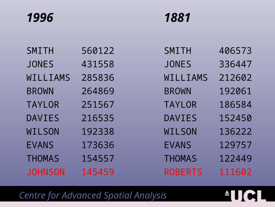
Let me take a simple example – surnames – if we rank the surnames from the most common to the least, then what we get from the 1996 UK electoral register is the following:

1 SMITH 5601222 JONES 4315583 WILLIAMS 2858364 BROWN 2648695 TAYLOR 2515676 DAVIES 2165357 WILSON 1923388 EVANS 1736369 THOMAS 15455710 JOHNSON 145459


Now let us plot the graph of frequency versus rank and then also transform this to a linear scale – for all 25630 names in the data


1996 1881

SMITH 560122 SMITH 406573

JONES 431558 JONES 336447

WILLIAMS 285836 WILLIAMS 212602

BROWN 264869 BROWN 192061

TAYLOR 251567 TAYLOR 186584

DAVIES 216535 DAVIES 152450

WILSON 192338 WILSON 136222

EVANS 173636 EVANS 129757

THOMAS 154557 THOMAS 122449

JOHNSON 145459 ROBERTS 111602


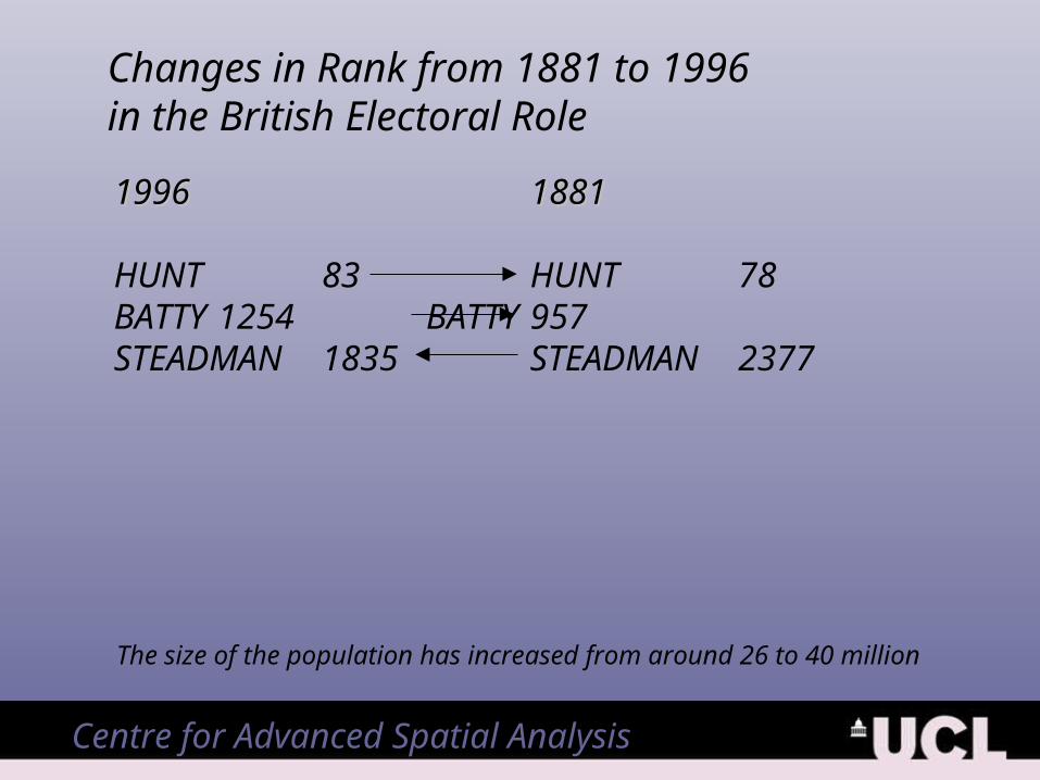
19961996 18811881

HUNT 83 HUNT 78BATTY 1254 BATTY 957STEADMAN 1835 STEADMAN 2377

Changes in Rank from 1881 to 1996 in the British Electoral Role

The size of the population has increased from around 26 to 40 million


2.2. City-Size/Rank-Size DynamicsCity-Size/Rank-Size DynamicsLo

g po

pula

tion

or L

og P

Log rank or Log r

111

rKrPPrrPPr logloglog 1

rKPr rKPr logloglog 1

The Strict Rank-Size Relation

The Variable Rank-Size Relation

The first popular demonstration of this relation was by Zipf in papers published in the 1930s and 1940s


log P

log r

P1

Growth or decline: pure scaling

The number of cities is expanding or contracting and all populations expand or contract

The number of cities is expanding or contracting and top populations are fixed.

The number of cities is fixed and all populations are expanding or contracting

mixed scaling:Cities expanding or contracting, populations expanding or contracting

Fixed or Variable Numbers of Cities and Populations


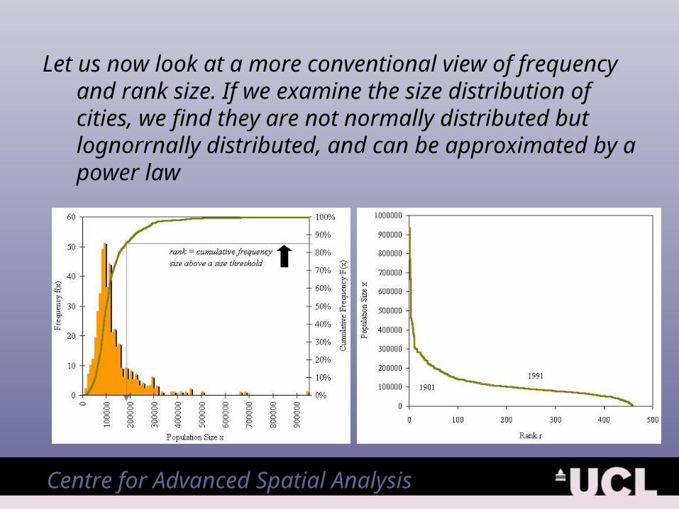
Let us now look at a more conventional view of frequency and rank size. If we examine the size distribution of cities, we find they are not normally distributed but lognorrnally distributed, and can be approximated by a power law


On log log paper, the counter cumulative or rank size distribution shows linearity over most of its length – and can be approximated – note approximated – by a power law. Here is an example for the distribution of over 20000 incorporated places from 1970 to 2000 from the US Census


This shows several things

Remarkable macro stability from 1970 to 2000

Classic lognormality consistent with the most basic of growth processes – proportionate random growth with no cities having greater growth rates that any other

A lack of economies of scale as cities get bigger which is counter conventional wisdom

Remarkable linearity in the long or fat or heavy tail which we can approximate with a power law as follows if we chop off the data at, say, 2500 population – we will do this


Parameter/Statistic 1970 1980 1990 2000

R Square 0.979 0.972 0.973 0.969

Intercept 16.790 16.891 17.090 17.360

Zipf-Exponent -0.986 -0.982 -0.995 -1.014


Notice the slopes of these straight lines – so close to 1

This is Zipf’s Law – termed after George Kingsley Zipf who first popularized it as the rank-size rule

Zipf’s Law … says that in a set of well-defined objects like words (or cities ? Or incomes? Pareto), the size of any object is inversely proportional to its rank; and in the strict Zipf case this is

This is the strict form because the power is -1 which gives it somewhat mystical properties but a more general form is the inverse power form

1 Krr

KPr

KrPr


3. Explanations – Lognormality, Stochasticity 3. Explanations – Lognormality, Stochasticity HierarchyHierarchy

The last 10 years has seen many attempts to explain scaling distributions such as these using various simple stochastic processes. Most do not take any account of the fact that cities compete – talk to each other.

In essence, the easiest is a model of proportionate effect or growth first used for economic systems by Gibrat in 1931 which leads to the lognormal distribution

There are many models based on this from Simon (1955) to Solomon and Blank (2001) – all variants on this theme – let me show you how this works very quickly


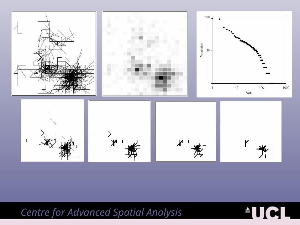
This is a good model to show the persistence of settlements, it is consistent with what we know about urban morphology in terms of fractal laws, but it is not spatial.

In fact to demonstrate how this model works let me run a short simulation based on independent events – cities on a 20 x 20 lattice using the Gibrat process – here it is – it will produce a lognormal but the volatility of the dynamics is suspect – an example of a simple phenomena simulated beautifully by a simple model – parsimony at its best which is the hall mark of science, but something that we know must be wrong !



I will digress a little here. Recently there has been a dramatic growth of network science due to people like Watts, Barabasi, Newman and so on. Essentially many of the results of scaling and lognormality that appear in city size, income, word distributions and so on, appear to hold for interactions associated with networks.

It is a simple matter to generate a model of a growing network where cities connect to each other according to what Barabasi calls ‘preferential attachment’ – ie the more the number of links in a hub, the more likely they are to get links. This is similar to Gibrat’s model of proportionate growth. It is no surprise that we get interactions distributed according to power laws or rank size as we can show




Three models – a digression

Most models which generate lognormal or scaling (power laws) in the long tail or heavy tail are based on the law of proportionate effect. We will identify 3 from many

Gibrat’s Model: Fixed Numbers of Cities

Most models which generate lognormal or scaling (power laws) in the long tail or heavy tail are based on the law of proportionate effect. We will identify 3 from many

Gibrat’s Model: Fixed Numbers of Cities

nitPtgtP iii ...,,2,1),()](1[)1(

),0()]0(1[...)]1(1)][(1[ iiii Pgtgtg

t

ii Pg0

)0()](1[


Gibrat’s Model with Lower Bound (the Solomon-Gabaix-Sornette Threshold) Fixed Numbers of Cities

T

TtPiftPtgtP iii

i

)(),()](1[)1(

nitPtgtP iii ...,,2,1),()](1[)1(

Gibrat’s Model with Lower Bound – Simon’s ModelExpanding (Contracting) Numbers of Cities

]1,,0[,...,,2,1,)1( zzifiijTtP jji

And there are the Barabasi models which add network links to the proportionate effects. See M. Batty (2006) Hierarchy in Cities and City Systems, in D. Pumain (Editor) Hierarchy in Natural and Social Sciences, Springer, Dordrecht, Netherlands, 143-168.


4. Volatility within Stability4. Volatility within Stability

What is so remarkable is the fact that we have such volatility within such macro stability – cities are shifting their positions all the time as we can see if we compare stable rank systems – population of US counties between 1940 and 2000

In essence the stochastic models generate too much volatility – and what we need is to add more inertia and of course to add space

Let me show this volatility by showing how ranks shift over this 60 year period


0

4

8

12

16

20

0 3 6 9

Rank-size of Population of US Counties 1940 and 2000with red plot showing 2000 populations but at 1940 ranks


5. Reworking Zipf: The US Urban System: The 5. Reworking Zipf: The US Urban System: The Emergence of CitiesEmergence of Cities

I am now going to look at the US, then the UK urban system. We have noted a number of data sets but we will only deal here with the top 100 towns or cities in terms of population size from 1790 to 2000. There are in fact 268 distinct cities that enter and leave the top 100 between these dates but the data is consistent in terms of definition.

So we are looking at the top of the rank-size hierarchy and in fact it is not until 1840 that we actually get 100 towns defined in the US Census. As we will see, the urban system is rapidly growing over this 210 years.


Now we are going to look at the dynamics from 1790 to 2001 in the classic way Zipf did and this is an updating of Zipf.

We have taken the top 100 places from Gibson’s Census Bureau Statistics which run from 1790 to 1990 and added to this the 2000 city populations

We have performed log log regressions to fit Zipf’s Law to these

We have then looked at the way cities enter and leave the top 100 giving a rudimentary picture of the dynamics of the urban system

We have visualized this dynamics in the many different ways but first we will show what Zipf did.


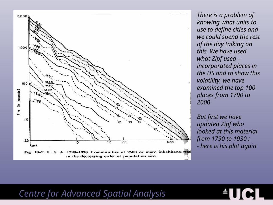
There is a problem of knowing what units to use to define cities and we could spend the rest of the day talking on this. We have used what Zipf used – incorporated places in the US and to show this volatility, we have examined the top 100 places from 1790 to 2000

But first we have updated Zipf who looked at this material from 1790 to 1930 :- here is his plot again


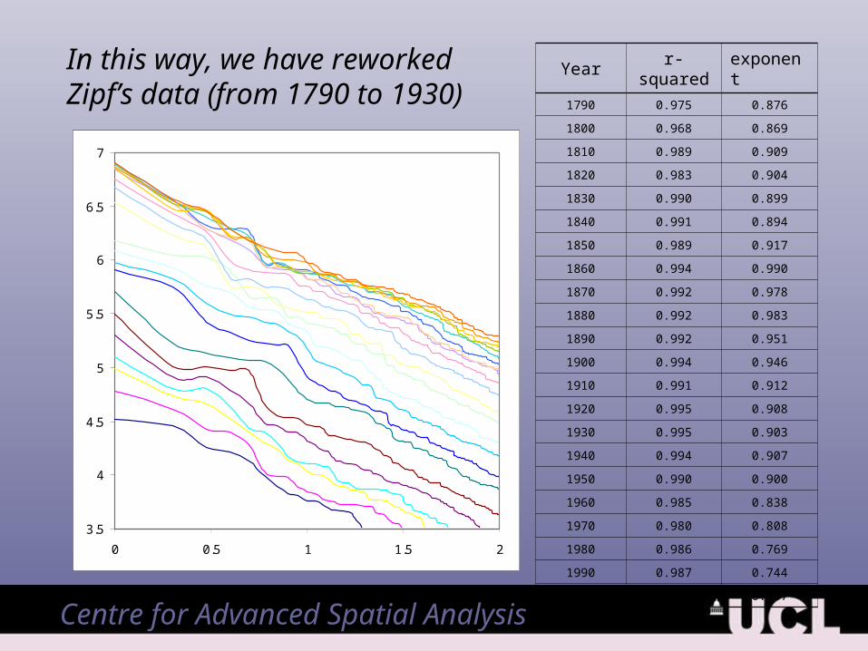
In this way, we have reworkedZipf’s data (from 1790 to 1930)

3.5

4

4.5

5

5.5

6

6.5

7

0 0.5 1 1.5 2

Year r-squared exponent

1790 0.975 0.876

1800 0.968 0.869

1810 0.989 0.909

1820 0.983 0.904

1830 0.990 0.899

1840 0.991 0.894

1850 0.989 0.917

1860 0.994 0.990

1870 0.992 0.978

1880 0.992 0.983

1890 0.992 0.951

1900 0.994 0.946

1910 0.991 0.912

1920 0.995 0.908

1930 0.995 0.903

1940 0.994 0.907

1950 0.990 0.900

1960 0.985 0.838

1970 0.980 0.808

1980 0.986 0.769

1990 0.987 0.744

2000 0.988 0.737


1000

10000

100000

1000000

10000000

1 Log Rank 10 100

Chicago

Houston

Los Angeles

RichmondVA

NorfolkVA

Boston

Baltimore

Charleston

NewYorkCity

Philadelphia

Log CitySize

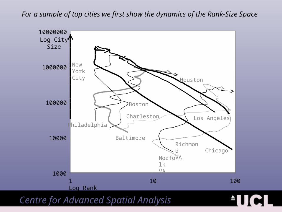
For a sample of top cities we first show the dynamics of the Rank-Size Space


We have also worked out how fast cities stay in the list & we callthese ‘half lives’

We can animatethese

0

20

40

60

80

100

1780 1800 1820 1840 1860 1880 1900 1920 1940 1960 1980 2000


6. The UK Urban System6. The UK Urban System

In the case of the US urban system, we had an expanding space of cities (except for the US county data which is a mutually exclusive subdivision of the US space)

However for the UK, the definition of cities is much more problematic. We do however have a good data set based on 458 local municipalities (for England, Scotland and Wales) which has consistent boundaries from 1901 to 2001.

So this, unlike the Zipf analysis, is for a fixed set of spaces where insofar as cities emerge or disappear, this is purely governed by their size.


3

3.5

4

4.5

5

5.5

6

6.5

0 0.5 1 1.5 2 2.5 3

1991

1901

Log of Rank

Log

of

Pop

ulat

ion

Here is the data – very similar stability at the macro level to the US data for counties and places but at the micro level….


-4.5

-4

-3.5

-3

-2.5

-2

-1.5

-1

0 0.5 1 1.5 2 2.5 3

1901

1991

Log of Rank

1991 Population based on 1901 Ranks

Log

of

Pop

ulat

ion

Sha

res

Here is an example of the shift in size and ranks over the last 100 years


Year t Correlation R2 Intercept Kt tKtP 101* Slope t

1901 0.879 6.547 3526157.772 -0.8171911 0.880 6.579 3801260.554 -0.8101921 0.887 6.604 4025650.857 -0.8121931 0.892 6.607 4046932.207 -0.8021941 0.865 6.532 3410371.276 -0.7401951 0.869 6.482 3034245.953 -0.7001961 0.830 6.414 2595897.640 -0.6511971 0.815 6.322 2101166.738 -0.6011981 0.816 6.321 2095242.746 -0.6011991 0.791 6.272 1872348.019 -0.577

This is what we get when we fit the rank size relation Pr=P1 r - to the data. Rather similar to the US data – flattening of the slope of the power law which probably implies decentralization or diffusion of population dominating trends towards centralization or concentration


0

200000

400000

600000

800000

1000000

1200000

1400000

1901 1911 1921 1931 1941 1951 1961 1971 1981 1991

Now we show the changes in population for the top ranked places from 1901 to 1991


And now we show the changes in rank for these places

0

20

40

60

80

100

120

140

1901 1911 1921 1931 1941 1951 1961 1971 1981 1991


7. Rank Clocks7. Rank Clocks

I think one of the most interesting innovations to examine these micro-dynamics is the rank clock which can be developed in various forms. Essentially we array the time around the perimeter of a circular clock and then plot the rank of any city or place along each finger of the clock for the appropriate time at which the city was so ranked.

Instead of plotting the rank, we could plot the population by ordering the populations according to their rank. For any time, the first ranked population would define the first city, then adding the second ranked population to the first would determine the second city position and so on


189019001910

1790 1800

1810

1820

1830

1840 Time

1850

1860

1870

18801920

1930

1940

1950

1960

1970

1980

1990

2000

Rank 1 20 40 60 80 100

Chicago

Houston

LA

RichmondVA

NorfolkVA

Boston Baltimore

Charleston

The Rank Clock for the US data


189019001910

1790 1800

1810

1820

1830

1840 Time

1850

1860

1870

18801920

1930

1940

1950

1960

1970

1980

1990

2000

(Log) Rank 1 10 100

Chicago

HoustonLA

Richmond VA

NorfolkVA

Boston Baltimore

CharlestonNY

Philly

The Log Rank Clockfor the US data


CamdenHackneyIslingtonLambethNewhamSouthwarkTower HamletsWandsworthWestminsterBarnetBrentBromleyCroydonEalingManchesterSalfordWiganLiverpoolSeftonWirralDoncasterSheffieldNewcastle SunderlandBirminghamCoventryDudleySandwellKirkleesLeedsWakefieldBristolEdinburghGlasgow

1901

1911

1921

1931

1941

1951

1961

1971

1981

1991

The Rank Clock forThe UK data


8. Next Steps8. Next Steps

The program to visualize many such data sets

Analysis of extinctions

Many cities and city systems

The analysis for firms and other scaling systemsetc. etc………….


Resources on these Kinds of ModelResources on these Kinds of Model http://www.casa.ucl.ac.uk/naru/portfolio/social.html

Arlinghaus, S. et al. (2003) Animated Time Lines: Co-ordination of Spatial and Temporal Information, Solstice , 14 (1) at http://www.arlinghaus.net/image/solstice/sum03/ andhttp://www.InstituteOfMathematicalGeography.org

Batty, M. and Shiode, N. (2003) Population Growth Dynamics in Cities, Countries and Communication Systems, In P. Longley and M. Batty (eds.), Advanced Spatial Analysis, Redlands, CA: ESRI Press (forthcoming). See http://www.casabook.com/

Batty, M. (2003) Commentary: The Geography of Scientific Citation, Environment and Planning A, 35, 761-765 at http://www.envplan.com/epa/editorials/a3505com.pdf


Academic Press, 1994 The MIT Press, 2005Academic Press, 1994 The MIT Press, 2005

http://www.casa.ucl.ac.uk/ http://www.casa.ucl.ac.uk/citations/

Documents

Centre for Advanced Spatial Analysis Tuesday, 24 January 2006 Said Business School CABDyN Seminar Cities and Complexity Explaining the Dynamics of Urban