Center for Turbulence ResearchAnnual Research Briefs 2010

263

LES of temporally evolving mixing layers byhigh-order filter schemes

By A. Hadjadj, H. C. Yee AND B. Sjogreen

1. Motivation and objective

Over the past decade, the use of computational fluid dynamics (CFD) in engineeringscience has increased, not only for fundamental understanding of complex compressibleturbulent physics, but also for the development and design of industrial devices. Owingto the recent progress in petascale computing, in tandem with advances in algorithmdevelopment for accurate direct numerical simulations (DNS) and large eddy simulations(LES) of shock-free compressible turbulence and turbulence with strong shocks, thistype of DNS and LES computation has gradually been able to tackle more complex flowsphysics. Advances in flow visualization tools have paved the way to extracting valuableinformation from the computed results containing hundreds of terabyte of data. Examplesinclude flows through internal propulsive nozzles with shock-wave propagation or soundemission from supersonic jets, and mixing and shock/boundary layer interactions.

Efficient and accurate DNS and LES simulations of the aforementioned flow physics,especially shock-wave/boundary layer interactions (SWBLI) for supersonic and hyper-sonic turbulence flows, are computationally very challenging due to the wide range oftemporal and spatial length scales. For turbulent flows, the only known route to generalhigh-fidelity flow simulations is through fully resolving all scales. The absence of scaleseparation makes it very difficult to take mathematical short cuts. State-of-the-art nu-merical methods for simulation of supersonic and hypersonic flows are designed to berobust enough to handle strong shock waves. However, these methods are not accurateenough to resolve a wide range of turbulent scales without additional improvement. Interms of turbulence modeling, there has been considerable progress in the developmentand usage of large eddy simulation (LES) for the simulation of turbulent flows in the pastfew decades. While a substantial amount of research has been carried out into modelingfor the LES of incompressible flows, applications to compressible flows have been signif-icantly fewer, due to the increased complexity introduced by the need to resolve a totalenergy equation, which introduces extra unclosed terms in addition to the subgrid-scalestresses that must be modeled in incompressible flows.

For the current investigation, the high-order nonlinear filter schemes with a pre- andpostprocessing step are selected due to the efficiency, accuracy and highly parallelizablenature of the construction (Yee & Sjogreen 2009). Studies in Yee & Sjogreen (2009) andYee et al. (2010) indicate that for turbulence with shock problems, an eighth-order spatialbase scheme in conjunction with a dissipative portion of WENO7 (WENO7fi) is moreaccurate than its fourth- and sixth-order counterparts. Studies found that employing en-tropy splitting (Yee et al. 2000; Sjogreen & Yee 2009; Honein & Moin 2004) of the inviscidflux derivative can stabilize the central base scheme for smooth flows. In addition, thissplitting is the most accurate among the aforementioned splitting methods. Indirectly,less numerical dissipation is needed when the split form is used. Unfortunately, entropysplitting is not suitable for problems with moderate and strong shocks as the split form

264 A. Hadjadj, H. C. Yee and B. Sjogreen

is not conservative. Due to the mixture of shock-free turbulence and turbulence withshocklets, for all of the computations shown later, the Ducros et al. (2000) splitting isemployed since a conservative splitting is more appropriate.

In this paper we report recent progress in the development and validation of LES com-putations of compressible turbulent mixing layers using high-order numerical schemes.The current research is motivated by the long-term overarching goal of developing nu-merical tools for reliable predictive capability of complex turbulent flows, especially forproblems including compressibility, heat transfer and real gas effects that interact withinstabilities, shocks and turbulence.

2. LES of temporally evolving compressible mixing layers

LES of temporally evolving mixing layers (TML) between two streams moving withopposite velocities is considered, with U1 = −U2 = ∆U/2. The three main characteristicsof compressible mixing layers are: 1) the self-similarity property, which is characterizedby linear growth of the layer as well as the mean velocities and turbulent statistics beingindependent of the downstream distance normalized by appropriate length and velocityscales; 2) the compressibility effects through turbulence damping and decrease of themixing-layer growth rate for high convective Mach numbers; and 3) the presence of alarge-scale structure with shocklets. These organized structures play an important rolein the dynamics of the mixing layer, its spreading and energy transport. The objective ofthe current investigation is to verify that the numerical methods used in this study arecapable of dealing with the three key points cited above. An other objective is to performand validate a well-resolved spatial large-eddy simulation to obtain accurate and reliabledata at higher Mach and Reynolds numbers.

2.1. Problem setupThe configuration of the temporally evolving mixing layer is shown in Figure 1. Five testcases (denoted LES-Ci, i = 1, .., 5) are carried out with different convective Mach num-bers ranging from the incompressible case Mc = 0.1 up to the supersonic one Mc = 1.5.The later corresponds to a highly compressible mixing layer, whereas the first two cases,Mc = 0.1 and Mc = 0.3, can be considered as quasi-incompressible and are used to com-pare with the experimental results of incompressible shear layer. All of the simulationsdescribed below are performed at an initial Reynolds number, Reω0 , based on the meanvelocity difference ∆U , the average viscosity of the free streams and the vorticity thick-ness δω0 of 800 with δw0 = 4 δθ0 , where δω = ∆U/〈∂u/∂y〉max is the vorticity thicknessof the shear layer, and δθ is the momentum thickness given by Eq. 2.2. Reω reachesvalues as large as 3× 105 at the end of the simulation, which is one order of magnitudehigher than the similar DNS and LES computations reported in the literature (Pan-tano & Sarkar 2002; Mahle et al. 2007; Foysi & Sarkar 2010). Table 1 summarizes thedetails of flow parameters for both LES and previous DNS data in the literature. Themean flow is initialized with a tangent hyperbolic profile for the streamwise velocity,u(y) = 1

2∆U tanh [y/(2 δθ0)], while the two other velocity components are set to zero. Inaddition to these mean values, three-dimensional turbulent fluctuations (u′, v′, w′) areimposed, while initial pressure and density are set constant. Since the simulation is tem-poral, the initial perturbations are added only once to the velocity field using a digitalfilter technique (Klein et al. 2003). This procedure utilizes the prescribed Reynolds stresstensor and length scales of the problem concerned to generate the corresponding fluc-tuating velocity field, taking into account the nature of autocorrelation function for the

LES of temporally evolving mixing layers 265

Lz

Lx

Ly

yx

z

stream 1

stream 2

Figure 1. Schematic configuration of temporal mixing layer

prevailing turbulence. The length scales are chosen as δw0 in each direction. The Reynoldsstress tensor is assumed to have a Gaussian shape with amplitudes taken similar to theexperimental peak intensities available for the incompressible mixing layer (Bell & Mehta1990).

Periodic boundary conditions are enforced in the streamwise (x) and spanwise (z)directions, while non-reflecting conditions are applied in both top and bottom boundaries(y direction). The use of a periodic boundary condition in the x direction corresponds tothe temporal formulation of mixing layer evolution, which is supposed to evolve only intime as it spreads in y.

2.2. Mesh requirementsSimilarly to Foysi & Sarkar (2010), a large computational domain of lengths Lx ×Ly × Lz = 1200 δθ0 × 370 δθ0 × 270 δθ0 is used with the corresponding mesh pointsNx ×Ny ×Nz = 512× 211× 131. The same grid system uniformly spaced in the x and zdirections and stretched in the y direction is employed for all cases considered. The HighResolution (HR) grid used in this study contains an order of magnitude fewer cells thanthat of the DNS of Pantano & Sarkar (2002) compared to the domain length. The em-phasis of the HR simulation is to produce an LES solution that predicts the trends of theDNS as well as experimental data for both quasi-incompressible and highly-compressiblemixing layers. To ensure that the computational domain in the x and z directions issufficiently wide, the two-point correlation functions are analyzed,

Rϕϕ (r) =N−kr∑k=1

ϕ′k ϕ′k+kr, kr = 0, 1, ...., N − 1, (2.1)

where r = kr∆, N is half of the number of grid points in the homogeneous directionswith grid size ∆ and ϕ′ represents the fluctuations of flow variables.

The computed two-point autocorrelation coefficients Rϕϕ(r)/Rϕϕ(0) (pressure as wellas velocity components) in the homogeneous directions (x and z) are reported in Figure2 as a function of the distance in the stream- and spanwise coordinates at the middle ofthe mixing layer (Ly/2) and at τ = 2500. The two part of the figure show that the flowvariables are sufficiently decorrelated over distances Lx/2 and Lz/2, thus ensuring thatthe streamwise as well as the spanwise extents of the computational domain are sufficientso as to not inhibit turbulence dynamics. Also, the length in y direction is selected to belarge enough for the flow to achieve a fully developed state. In terms of turbulent lengthscales, the Kolmogorov length scale η and an average (isotropic)Taylor micro-scale λ are

266 A. Hadjadj, H. C. Yee and B. Sjogreen

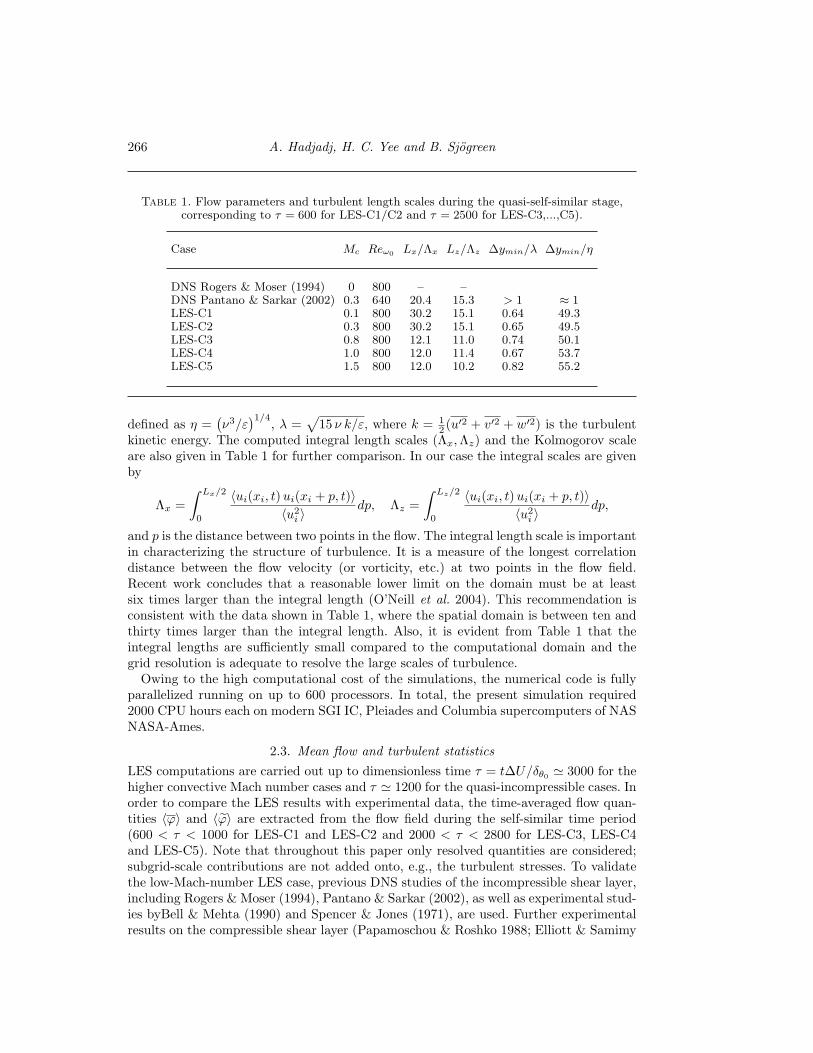
Table 1. Flow parameters and turbulent length scales during the quasi-self-similar stage,corresponding to τ = 600 for LES-C1/C2 and τ = 2500 for LES-C3,...,C5).

Case Mc Reω0 Lx/Λx Lz/Λz ∆ymin/λ ∆ymin/η

DNS Rogers & Moser (1994) 0 800 – –DNS Pantano & Sarkar (2002) 0.3 640 20.4 15.3 > 1 ≈ 1LES-C1 0.1 800 30.2 15.1 0.64 49.3LES-C2 0.3 800 30.2 15.1 0.65 49.5LES-C3 0.8 800 12.1 11.0 0.74 50.1LES-C4 1.0 800 12.0 11.4 0.67 53.7LES-C5 1.5 800 12.0 10.2 0.82 55.2

defined as η =(ν3/ε

)1/4, λ =√

15 ν k/ε, where k = 12 (u′2 + v′2 + w′2) is the turbulent

kinetic energy. The computed integral length scales (Λx,Λz) and the Kolmogorov scaleare also given in Table 1 for further comparison. In our case the integral scales are givenby

Λx =∫ Lx/2

0

〈ui(xi, t)ui(xi + p, t)〉〈u2

i 〉dp, Λz =

∫ Lz/2

0

〈ui(xi, t) ui(xi + p, t)〉〈u2

i 〉dp,

and p is the distance between two points in the flow. The integral length scale is importantin characterizing the structure of turbulence. It is a measure of the longest correlationdistance between the flow velocity (or vorticity, etc.) at two points in the flow field.Recent work concludes that a reasonable lower limit on the domain must be at leastsix times larger than the integral length (O’Neill et al. 2004). This recommendation isconsistent with the data shown in Table 1, where the spatial domain is between ten andthirty times larger than the integral length. Also, it is evident from Table 1 that theintegral lengths are sufficiently small compared to the computational domain and thegrid resolution is adequate to resolve the large scales of turbulence.

Owing to the high computational cost of the simulations, the numerical code is fullyparallelized running on up to 600 processors. In total, the present simulation required2000 CPU hours each on modern SGI IC, Pleiades and Columbia supercomputers of NASNASA-Ames.

2.3. Mean flow and turbulent statisticsLES computations are carried out up to dimensionless time τ = t∆U/δθ0 ' 3000 for thehigher convective Mach number cases and τ ' 1200 for the quasi-incompressible cases. Inorder to compare the LES results with experimental data, the time-averaged flow quan-tities 〈ϕ〉 and 〈ϕ〉 are extracted from the flow field during the self-similar time period(600 < τ < 1000 for LES-C1 and LES-C2 and 2000 < τ < 2800 for LES-C3, LES-C4and LES-C5). Note that throughout this paper only resolved quantities are considered;subgrid-scale contributions are not added onto, e.g., the turbulent stresses. To validatethe low-Mach-number LES case, previous DNS studies of the incompressible shear layer,including Rogers & Moser (1994), Pantano & Sarkar (2002), as well as experimental stud-ies byBell & Mehta (1990) and Spencer & Jones (1971), are used. Further experimentalresults on the compressible shear layer (Papamoschou & Roshko 1988; Elliott & Samimy

LES of temporally evolving mixing layers 267

0 0.1 0.2 0.3 0.4 0.5-0.2

0

0.2

0.4

0.6

0.8

u’v’w’p’

0 0.1 0.2 0.3 0.4 0.5-0.2

0

0.2

0.4

0.6

0.8

u’v’w’p’

Figure 2. Streamwise and spanwise autocorrelation functions for LES-C5 at τ = 2500.

0 100 200 300 400 500 600 7000

3

6

9

12

15DNS Pantano & SarkarLES-C2

-3 -2 -1 0 1 2 3-0.6

-0.3

0

0.3

0.6Bell & MehtaSpencer & Jones

DNS - Pantano et al., Mc=0.3

LES, Mc=0.1

LES, Mc=0.3

Exp.

Figure 3. (left) Time evolution of normalized momentum thickness for LES-C2 compared tothe DNS of Pantano & Sarkar (2002) for Mc = 0.3. (right) Comparison of normalized meanstreamwise velocity for LES-C1 and LES-C2.

1990; Barre et al. 1997; Chambres et al. 1998) and DNS results obtained by Pantano &Sarkar (2002) are used to compare with the high-Mach-number simulations.

As recommended by Rogers & Moser (1994), the momentum thickness δθ is used forself-similar scaling rather than the vorticity thickness δω, because it is less sensitive tostatistical noise as it is an integral quantity evolving smoothly in time, whereas δω isobtained from the derivative of the mean velocity and may exhibit oscillations duringflow evolution. Therefore, the time evolution of the momentum thickness of the flowcalculated using the definition

δθ =∫ +∞

−∞

ρ

ρref

(14− u2

∆U2

)dy (2.2)

is shown in Figure 3. Excellent agreement with the DNS simulation is obtained and thelinear slope is recovered after a short transient, showing the self-similar state of the mixinglayer. The growth rate d(δθ/δθ0)/dτ (slope of the linear curve fit) for this case is foundto be 0.016. The ratio of vorticity thickness to momentum thickness (Dω = δω/δθ ' 4.5)with Reω = 603391 at τmax ' 1200. This is in excellent agreement with the DNS growthrate of the quasi-incompressible case with Mc = 0.3 of Pantano & Sarkar (2002). Notethat in Eq. 2.2, (. )ref represents the reference state which is the arithmetic mean of thefree streams 1 and 2.

268 A. Hadjadj, H. C. Yee and B. Sjogreen

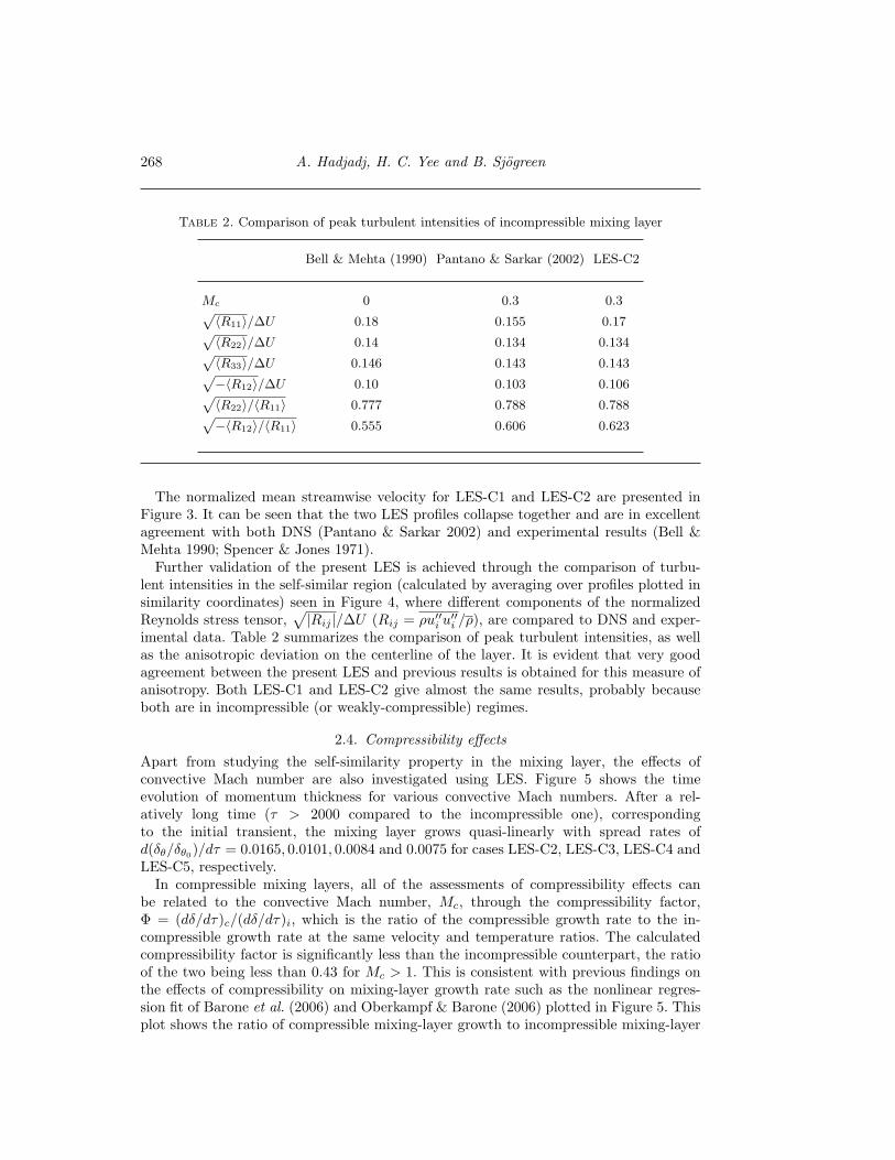
Table 2. Comparison of peak turbulent intensities of incompressible mixing layer

Bell & Mehta (1990) Pantano & Sarkar (2002) LES-C2

Mc 0 0.3 0.3p〈R11〉/∆U 0.18 0.155 0.17p〈R22〉/∆U 0.14 0.134 0.134p〈R33〉/∆U 0.146 0.143 0.143p−〈R12〉/∆U 0.10 0.103 0.106p〈R22〉/〈R11〉 0.777 0.788 0.788p−〈R12〉/〈R11〉 0.555 0.606 0.623

The normalized mean streamwise velocity for LES-C1 and LES-C2 are presented inFigure 3. It can be seen that the two LES profiles collapse together and are in excellentagreement with both DNS (Pantano & Sarkar 2002) and experimental results (Bell &Mehta 1990; Spencer & Jones 1971).

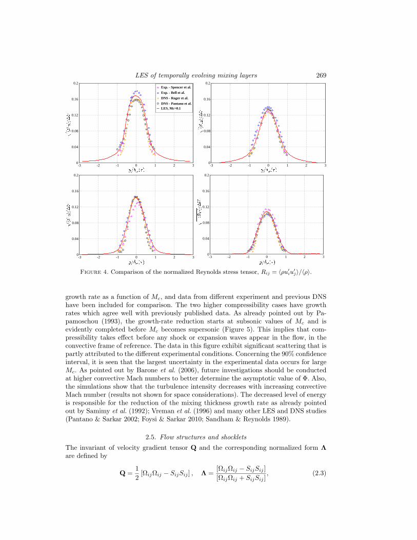
Further validation of the present LES is achieved through the comparison of turbu-lent intensities in the self-similar region (calculated by averaging over profiles plotted insimilarity coordinates) seen in Figure 4, where different components of the normalizedReynolds stress tensor,

√|Rij |/∆U (Rij = ρu′′i u′′i /ρ), are compared to DNS and exper-

imental data. Table 2 summarizes the comparison of peak turbulent intensities, as wellas the anisotropic deviation on the centerline of the layer. It is evident that very goodagreement between the present LES and previous results is obtained for this measure ofanisotropy. Both LES-C1 and LES-C2 give almost the same results, probably becauseboth are in incompressible (or weakly-compressible) regimes.

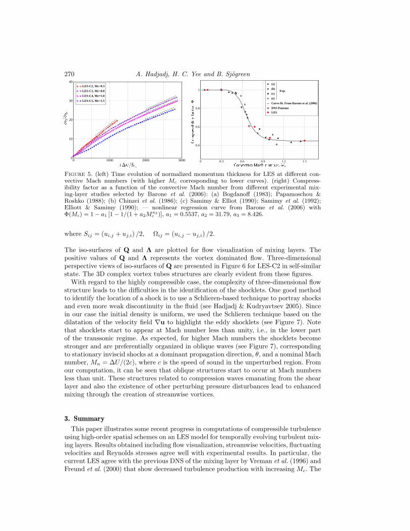
2.4. Compressibility effectsApart from studying the self-similarity property in the mixing layer, the effects ofconvective Mach number are also investigated using LES. Figure 5 shows the timeevolution of momentum thickness for various convective Mach numbers. After a rel-atively long time (τ > 2000 compared to the incompressible one), correspondingto the initial transient, the mixing layer grows quasi-linearly with spread rates ofd(δθ/δθ0)/dτ = 0.0165, 0.0101, 0.0084 and 0.0075 for cases LES-C2, LES-C3, LES-C4 andLES-C5, respectively.

In compressible mixing layers, all of the assessments of compressibility effects canbe related to the convective Mach number, Mc, through the compressibility factor,Φ = (dδ/dτ)c/(dδ/dτ)i, which is the ratio of the compressible growth rate to the in-compressible growth rate at the same velocity and temperature ratios. The calculatedcompressibility factor is significantly less than the incompressible counterpart, the ratioof the two being less than 0.43 for Mc > 1. This is consistent with previous findings onthe effects of compressibility on mixing-layer growth rate such as the nonlinear regres-sion fit of Barone et al. (2006) and Oberkampf & Barone (2006) plotted in Figure 5. Thisplot shows the ratio of compressible mixing-layer growth to incompressible mixing-layer

LES of temporally evolving mixing layers 269

-3 -2 -1 0 1 2 30

0.04

0.08

0.12

0.16

0.2Exp. - Spencer et al.

Exp. - Bell et al.

DNS - Roger et al.

DNS - Pantano et al.LES, Mc=0.1

-3 -2 -1 0 1 2 30

0.04

0.08

0.12

0.16

0.2

-3 -2 -1 0 1 2 30

0.04

0.08

0.12

0.16

0.2

-3 -2 -1 0 1 2 30

0.04

0.08

0.12

0.16

0.2

Figure 4. Comparison of the normalized Reynolds stress tensor, Rij = 〈ρu′iu

′j〉/〈ρ〉.

growth rate as a function of Mc, and data from different experiment and previous DNShave been included for comparison. The two higher compressibility cases have growthrates which agree well with previously published data. As already pointed out by Pa-pamoschou (1993), the growth-rate reduction starts at subsonic values of Mc and isevidently completed before Mc becomes supersonic (Figure 5). This implies that com-pressibility takes effect before any shock or expansion waves appear in the flow, in theconvective frame of reference. The data in this figure exhibit significant scattering that ispartly attributed to the different experimental conditions. Concerning the 90% confidenceinterval, it is seen that the largest uncertainty in the experimental data occurs for largeMc. As pointed out by Barone et al. (2006), future investigations should be conductedat higher convective Mach numbers to better determine the asymptotic value of Φ. Also,the simulations show that the turbulence intensity decreases with increasing convectiveMach number (results not shown for space considerations). The decreased level of energyis responsible for the reduction of the mixing thickness growth rate as already pointedout by Samimy et al. (1992); Vreman et al. (1996) and many other LES and DNS studies(Pantano & Sarkar 2002; Foysi & Sarkar 2010; Sandham & Reynolds 1989).

2.5. Flow structures and shocklets

The invariant of velocity gradient tensor Q and the corresponding normalized form Λare defined by

Q =12

[ΩijΩij − SijSij ] , Λ =[ΩijΩij − SijSij ][ΩijΩij + SijSij ]

, (2.3)

270 A. Hadjadj, H. C. Yee and B. Sjogreen

0 1000 2000 30000

10

20

30

40LES-C2, Mc=0.3

LES-C3, Mc=0.8

LES-C4, Mc=1.0

LES-C5, Mc=1.5

0 0.3 0.6 0.9 1.2 1.5

0.4

0.6

0.8

1

(a)

(b)

(c)

(e)

Curve fit. From Barone et al. (2006)

DNS Pantano

LES

Exp.

Figure 5. (left) Time evolution of normalized momentum thickness for LES at different con-vective Mach numbers (with higher Mc corresponding to lower curves). (right) Compress-ibility factor as a function of the convective Mach number from different experimental mix-ing-layer studies selected by Barone et al. (2006): (a) Bogdanoff (1983); Papamoschou &Roshko (1988); (b) Chinzei et al. (1986); (c) Samimy & Elliot (1990); Samimy et al. (1992);Elliott & Samimy (1990); — nonlinear regression curve from Barone et al. (2006) withΦ(Mc) = 1− a1 [1− 1/(1 + a2M

a3c )], a1 = 0.5537, a2 = 31.79, a3 = 8.426.

where Sij = (ui,j + uj,i) /2, Ωij = (ui,j − uj,i) /2.

The iso-surfaces of Q and Λ are plotted for flow visualization of mixing layers. Thepositive values of Q and Λ represents the vortex dominated flow. Three-dimensionalperspective views of iso-surfaces of Q are presented in Figure 6 for LES-C2 in self-similarstate. The 3D complex vortex tubes structures are clearly evident from these figures.

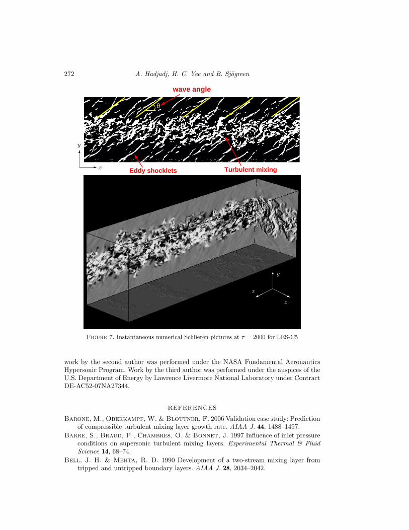
With regard to the highly compressible case, the complexity of three-dimensional flowstructure leads to the difficulties in the identification of the shocklets. One good methodto identify the location of a shock is to use a Schlieren-based technique to portray shocksand even more weak discontinuity in the fluid (see Hadjadj & Kudryavtsev 2005). Sincein our case the initial density is uniform, we used the Schlieren technique based on thedilatation of the velocity field ∇u to highlight the eddy shocklets (see Figure 7). Notethat shocklets start to appear at Mach number less than unity, i.e., in the lower partof the transsonic regime. As expected, for higher Mach numbers the shocklets becomestronger and are preferentially organized in oblique waves (see Figure 7), correspondingto stationary inviscid shocks at a dominant propagation direction, θ, and a nominal Machnumber, Mn = ∆U/(2c), where c is the speed of sound in the unperturbed region. Fromour computation, it can be seen that oblique structures start to occur at Mach numbersless than unit. These structures related to compression waves emanating from the shearlayer and also the existence of other perturbing pressure disturbances lead to enhancedmixing through the creation of streamwise vortices.

3. Summary

This paper illustrates some recent progress in computations of compressible turbulenceusing high-order spatial schemes on an LES model for temporally evolving turbulent mix-ing layers. Results obtained including flow visualization, streamwise velocities, fluctuatingvelocities and Reynolds stresses agree well with experimental results. In particular, thecurrent LES agree with the previous DNS of the mixing layer by Vreman et al. (1996) andFreund et al. (2000) that show decreased turbulence production with increasing Mc. The

LES of temporally evolving mixing layers 271

Figure 6. Iso-surface of Q = 0.01Qmax colored by density at τ = 1000 and for LES-C2

-

6

x

y

-

6

x

z

-

6

z

y

x

present study serves as a validation of the performance of the improved filter schemes ofYee & Sjogreen (2009) on a representative complex compressible turbulent flow consistingof a wide range of flow speeds.

AcknowledgementsThe first author would like to acknowledge the financial support from CTR and alsothrough the DOE/SciDAC SAP grant DE-AI02-06ER25796. Special thanks to M. Rogersand A. Wray for their valuable discussions during the course of this research. Part of the

272 A. Hadjadj, H. C. Yee and B. Sjogreen

-

6

x

y

wave angle

Turbulent mixingEddy shocklets

θ

Figure 7. Instantaneous numerical Schlieren pictures at τ = 2000 for LES-C5

HHHj

6y

z

x

work by the second author was performed under the NASA Fundamental AeronauticsHypersonic Program. Work by the third author was performed under the auspices of theU.S. Department of Energy by Lawrence Livermore National Laboratory under ContractDE-AC52-07NA27344.

REFERENCES

Barone, M., Oberkampf, W. & Blottner, F. 2006 Validation case study: Predictionof compressible turbulent mixing layer growth rate. AIAA J. 44, 1488–1497.

Barre, S., Braud, P., Chambres, O. & Bonnet, J. 1997 Influence of inlet pressureconditions on supersonic turbulent mixing layers. Experimental Thermal & FluidScience 14, 68–74.

Bell, J. H. & Mehta, R. D. 1990 Development of a two-stream mixing layer fromtripped and untripped boundary layers. AIAA J. 28, 2034–2042.

LES of temporally evolving mixing layers 273

Bogdanoff, D. W. 1983 Compressibility effects in turbulent shear layers. AIAA J. 21,926–927.

Chambres, O., Barre, S. & Bonnet, J. 1998 Detailed turbulence characteristics ofa highly compressible supersonic turbulent plane mixing layer. J. Fluid Mech. .

Chinzei, N., Masua, G., Komuro, T., Murakami, A. & Kudou, K. 1986 Spreadingof two-stream supersonic turbulent mixing layers. Phys. Fluids 29, 1345–1347.

Ducros, F., Laporte, F., Souleres, T., Guinot, V., Moinat, P. & Caruelle, B.2000 High-order fluxes for conservative skew-symmetric-like schemes in structuredmeshes: Application to compressible flows. J. Comput. Phys. 16, 114–139.

Elliott, G. & Samimy, M. 1990 Compressibility effects in free shear layers. Phys.Fluids 2, 1231–1240.

Foysi, H. & Sarkar, S. 2010 The compressible mixing layer: an LES study. Theor.Comp. Fluid Dyn. 24, 565–588.

Freund, J. B., Lele, S. K. & Moin, P. 2000 Compressibility effects in a turbulentannular mixing layer. Part 1. turbulence and growth rate. J. Fluid Mech. 421, 229–267.

Hadjadj, A. & Kudryavtsev, A. 2005 Computation and flow visualization in highspeed aerodynamics. J. Turbulence 6, 33–81.

Honein, A. & Moin, P. 2004 Higher entropy conservation and numerical stability ofcompressible turbulence simulations. J. Comput. Phys. 201, 531–545.

Klein, M. ., Sadiki, A. & Janicka, J. 2003 A digital filter based generation of inflowdata for spatially developing direct numerical or large-eddy simulation. J. Comput.Phys. 186, 652–665.

Mahle, I., Sesterhenn, J. & Friedrich, R. 2007 Turbulent mixing in temporalcompressible shear layers involving detailed diffusion processes. J. Turbulence 8,1–12.

Oberkampf, W. L. & Barone, M. 2006 Measures of agreement between computationand experiment: Validation metrics. J. Comp. Phys. 217, 5–36.

O’Neill, P. L., Nicolaides, D., Honnery, D. & Soria, J. 2004 Autocorrelationfunctions and the determination of integral length with reference to experimental andnumerical data. In 15th Australasian Fluid Mech. Conf.. Univ. of Sydney, Australia.

Pantano, C. & Sarkar, S. 2002 A study of compressible effects in the high-speedturbulent shear layer using direct simulation. J. Fluid Mech. 451, 329–371.

Papamoschou, D. 1993 Model for entropy production and pressure variation in confinedturbulent mixing layer. AIAA J. 31, 1643–1650.

Papamoschou, D. & Roshko, A. 1988 The compressible turbulent shear layer: Anexperimental study. J. Fluid Mech. 197, 453–477.

Rogers, M. M. & Moser, R. D. 1994 Direct simulation of a self-similar turbulentmixing layer. Phys. Fluids 6, 903–923.

Samimy, M. & Elliot, G. 1990 Effect of compressibility on the characteristics of freeshear layer. AIAA J. 28, 439–445.

Samimy, M., Reeder, M. & Elliott, G. 1992 Compressibility effects on large struc-tures in free shear flows. Phys. Fluids 4, 1251–1258.

Sandham, N. D. & Reynolds, W. C. 1989 A numerical investigation of the compress-ible mixing layer. In Stanford Rep. TF-45 .

Sjogreen, B. & Yee, H. C. 2009 On skew-symmetric splitting of the Euler equations.In EUNUMATH-09 Conference.

274 A. Hadjadj, H. C. Yee and B. Sjogreen

Spencer, B. W. & Jones, B. 1971 Statistical investigation of pressure and velocityfields in the turbulent two-stream mixing layer. In AIAA Paper 71-613 .

Vreman, B., Sandham, N. & Luo, K. 1996 Compressible mixing layer growth rateand turbulence characteristics. J. Fluid Mech. 320, 235–258.

Yee, H. & Sjogreen, B. 2009 High order filter methods for wide range of compressibleflow speeds. In ICOSAHOM 09 (International Conference on Spectral and HighOrder Methods), June 22-26 . Trondheim, Norway.

Yee, H., Sjogreen, B. & Hadjadj, A. 2010 Comparative study of high-order schemesfor LES of temporal-evolving mixing layers. In ASTRONUM-2010, June 13- 18 . SanDiego, Calif.

Yee, H., Vinokur, M. & Djomehri, M. 2000 Entropy splitting and numerical dissi-pation. J. Comput. Phys. 162, 33–81.